


1. Introduction
Low-density jets and their stability have been a topic of interest for many years due to one of the archetypes of flows having global oscillations. The globally unstable low-density jet has two distinct features, viz. narrow peaks in the frequency spectrum due to the appearance of regular periodic structure in the jet and a dramatic mixing in the near field, compared with the globally stable jet (Sreenivasan, Raghu & Kyle Reference Sreenivasan, Raghu and Kyle1989; Monkewitz et al. Reference Monkewitz, Bechert, Barsikow and Lehmann1990; Kyle & Sreenivasan Reference Kyle and Sreenivasan1993; Hallberg & Strykowski Reference Hallberg and Strykowski2006).
Based on the experimental studies, it is now understood that the significant parameters controlling the global oscillatory state in low-density jets are the jet Mach number ( $M$), the jet Reynolds number ( $Re$), the non-dimensional momentum thickness of the inlet velocity profile ( $D/\theta _0$, where $D$ is a nozzle diameter), the ratio of jet to ambient density ( $S$) and the ambient coflow or counterflow (Sreenivasan et al. Reference Sreenivasan, Raghu and Kyle1989; Monkewitz et al. Reference Monkewitz, Bechert, Barsikow and Lehmann1990; Kyle & Sreenivasan Reference Kyle and Sreenivasan1993; Hallberg et al. Reference Hallberg, Srinivasan, Gorse and Strykowski2007; Zhu, Gupta & Li Reference Zhu, Gupta and Li2017). The early work of Monkewitz & Sohn (Reference Monkewitz and Sohn1988) demonstrated that the global oscillations in low-density jets are related to the absolute instability of low-density jets. Subsequent stability studies investigated the effect of parameters ( $M, Re, D/\theta _0$, and coflow or counterflow) on the absolute instability of low-density jets (Monkewitz & Sohn Reference Monkewitz and Sohn1988; Jendoubi & Strykowski Reference Jendoubi and Strykowski1994; Lesshafft & Huerre Reference Lesshafft and Huerre2007; Nichols, Schmid & Riley Reference Nichols, Schmid and Riley2007; Srinivasan, Hallberg & Strykowski Reference Srinivasan, Hallberg and Strykowski2010). Direct numerical simulation (DNS) and large eddy simulation (LES) of low-density jets using synthetic inlet velocity and density profiles have reproduced the experimental results qualitatively (Lesshafft et al. Reference Lesshafft, Huerre, Sagaut and Terracol2006; Lesshafft, Huerre & Sagaut Reference Lesshafft, Huerre and Sagaut2007; Nichols et al. Reference Nichols, Schmid and Riley2007; Foysi, Mellado & Sarkar Reference Foysi, Mellado and Sarkar2010; Boguslawski, Tyliszczak & Wawrzak Reference Boguslawski, Tyliszczak and Wawrzak2016). Stability and DNS studies showed that the baroclinic torque is responsible for the global oscillations in low-density jets (Lesshafft & Huerre Reference Lesshafft and Huerre2007; Lesshafft et al. Reference Lesshafft, Huerre and Sagaut2007). Experimental studies demonstrated that the global oscillations in low-density jets could be altered using coflow (Hallberg et al. Reference Hallberg, Srinivasan, Gorse and Strykowski2007) and acoustic excitation (Hallberg & Strykowski Reference Hallberg and Strykowski2008; Li & Juniper Reference Li and Juniper2013).
Experimental studies on rectangular low-density jets using helium–air mixtures exhibit global oscillations below the critical density ratio of 0.7 (Raynal et al. Reference Raynal, Harion, Favre-Marinet and Binder1996), whereas the critical density ratio for hot air jets injected into a cold air surrounding is 0.9 (Yu & Monkewitz Reference Yu and Monkewitz1993). Raynal et al. (Reference Raynal, Harion, Favre-Marinet and Binder1996) demonstrated using synthetic velocity and density base profiles (hyperbolic tangent profiles) that the absolute growth rate increases with a decrease in the relative distance between the inflection points of the velocity and density profile and reaches a maximum when the inflection points coincide. The relative distance between the inflection points is larger for helium jets than hot jets, and they hypothesized that this might be a reason for the lower critical density ratio for the helium–air jets compared with the hot jets. Similar results are observed for round low-density jets (Nichols et al. Reference Nichols, Schmid and Riley2007; Srinivasan et al. Reference Srinivasan, Hallberg and Strykowski2010). Based on sensitivity studies, Lesshafft & Marquet (Reference Lesshafft and Marquet2010) showed that the absolute instability of a jet is enhanced by (i) a strong velocity gradient in the low-velocity region of the shear layer and (ii) a step-like density variation near the maximum shear. They showed that homogeneous jets ( $S=1$) could also be absolutely unstable for specific velocity profiles.
Coenen and co-workers (Coenen, Sevilla & Sánchez Reference Coenen, Sevilla and Sánchez2008; Coenen & Sevilla Reference Coenen and Sevilla2012) carried out spatiotemporal stability studies on low-density jets using base flows close to the experimental conditions. They have used the laminar axisymmetric boundary layer equations to obtain the jet inlet velocity profiles and their downstream evolution. The inviscid stability results (Coenen et al. Reference Coenen, Sevilla and Sánchez2008) based on the boundary layer base flows predicted that the critical density ratio of low-density jets with  $D/\theta _0 \approx 20$ is 0.9, which is higher than the maximum critical density ratio of 0.7 reported from model profiles (hyperbolic tangent profiles). The viscous stability results showed that the critical density ratio of hot jets is higher than the isothermal helium–air jets indicating that the hot jets are more unstable than the helium–air jets, which is consistent with experimental results (Coenen & Sevilla Reference Coenen and Sevilla2012). Large eddy simulations of hot jets with the Blasius inlet velocity profiles are in better agreement with experimental results than the hot jets with hyperbolic inlet velocity profiles (Boguslawski et al. Reference Boguslawski, Tyliszczak and Wawrzak2016).
Studies by Raynal et al. (Reference Raynal, Harion, Favre-Marinet and Binder1996), Coenen et al. (Reference Coenen, Sevilla and Sánchez2008), Lesshafft & Marquet (Reference Lesshafft and Marquet2010) and Coenen & Sevilla (Reference Coenen and Sevilla2012) demonstrated that  $D/\theta$, which is an integral parameter of the velocity/density profile, is an inadequate parameter for the stability characteristics. The precise shapes of the velocity and density profiles are essential for computing the stability characteristics accurately. Most of the stability studies in the literature use synthetic/model velocity and density profiles as a base state, and in numerical simulations (DNS), synthetic velocity and density profiles are used as the inlet conditions to simulate low-density jets. The synthetic velocity and density profiles are either given independently or related through the Crocco–Busemann relation in the above studies. A summary of the base state velocity and density profiles (inlet and flow field) used in the stability of low-density jets is given in table 1.
Table 1. Summary of base state velocity and density (light jets)/temperature (hot jets) profiles used in stability studies on low-density jets. The BL solution and C–B relation denote profiles from the boundary layer equations and the Crocco–Busemann relation, respectively, whereas the N–S base and N–S mean denote base flow and mean flow from the Navier–Stokes equations, respectively.

The theory for predicting a nonlinear global mode and its characteristics from a local spatiotemporal stability analysis is favourably compared with experimental results (Chomaz Reference Chomaz2004, Reference Chomaz2005). The criteria for the onset of a nonlinear global mode and its frequency depends on the nature of the absolutely unstable region observed in the local analysis. A pocket of the absolutely unstable region away from the nozzle exit was shown to excite a nonlinear global mode, and at critical conditions, the corresponding global frequency matches with the absolute frequency ( $\omega _{0,i}$) of the location where the absolute growth rate changes from a negative to positive (Lesshafft et al. Reference Lesshafft, Huerre, Sagaut and Terracol2006). The absolutely unstable region bounded by the nozzle exit required a minimum length of the absolutely unstable region to sustain a nonlinear global mode, and at critical conditions, the frequency of global oscillations is equal to the absolute frequency at the nozzle exit (Lesshafft et al. Reference Lesshafft, Huerre, Sagaut and Terracol2006, Reference Lesshafft, Huerre and Sagaut2007; Coenen & Sevilla Reference Coenen and Sevilla2012).
The spatiotemporal stability results of Coenen et al. (Reference Coenen, Sevilla and Sánchez2008) showed that the absolute growth rate of the helical mode is higher than the axisymmetric mode for low-density jets with near parabolic velocity profiles ( $D/\theta _0 \approx 15$). The range of $D/\theta _0$ at which the helical mode is predicted to be dominant over the axisymmetric mode from the stability analysis is lower than the range of $D/\theta _0$ studied in experiments (Kyle & Sreenivasan Reference Kyle and Sreenivasan1993; Hallberg & Strykowski Reference Hallberg and Strykowski2006). Global stability analysis (Coenen et al. Reference Coenen, Lesshafft, Garnaud and Sevilla2017) and DNS (Lendínez Reference Lendínez2018) of low-density jets with parabolic velocity profiles ( $D/\theta _0 = 15$) predicted that the jet is globally unstable for the axisymmetric mode. Note that only axisymmetric modes were considered in the global stability analysis and DNS. Hence, it is not known whether the helical mode is globally unstable for low-density jets with parabolic velocity profiles. Satti & Agrawal (Reference Satti and Agrawal2006) investigated the role of gravity in helium jets (both buoyant and inertial jets) by numerical simulations using the unsteady axisymmetric laminar Navier–Stokes equations. They showed that the inertial helium jet with the parabolic velocity profile at $Re = 1600$ ( $Re = \rho ^*_j U^*_j D/\mu ^*_j$, where $\rho ^*_j, U^*_j$ and $\mu ^*_j$ are dimensional density, velocity and dynamic viscosity at the nozzle exit centreline, respectively) exhibits global oscillations. The Reynolds number of this globally unstable jet is much lower than the critical Reynolds number ( $Re \approx 3370$) predicted by the global stability analysis (Coenen et al. Reference Coenen, Lesshafft, Garnaud and Sevilla2017) and the critical Reynolds number ( $Re \approx 2300$) from the DNS (Lendínez Reference Lendínez2018). Recently, based on experimental studies, Ren & Li (Reference Ren and Li2018a,Reference Ren and Lib) reported global helical oscillations in low-density jets with thick shear layers. They observed that global helical oscillations are weaker than the global axisymmetric oscillations. Unfortunately, only the abstract of this work is available, and there is no information available regarding the range of parameters ( $Re, S$ and $D/\theta _0$) at which the global helical oscillations are possible. This experimental result supports the spatiotemporal stability result of Coenen et al. (Reference Coenen, Sevilla and Sánchez2008).
1.1. Motivation and objective
The available stability and numerical results in the literature related to low-density jets with parabolic velocity profiles are not consistent with each other. All the experimental studies on low-density jets in the literature deal with inlet velocity profiles far from parabolic (Sreenivasan et al. Reference Sreenivasan, Raghu and Kyle1989; Monkewitz et al. Reference Monkewitz, Bechert, Barsikow and Lehmann1990; Kyle & Sreenivasan Reference Kyle and Sreenivasan1993; Hallberg & Strykowski Reference Hallberg and Strykowski2006; Li & Juniper Reference Li and Juniper2013; Zhu et al. Reference Zhu, Gupta and Li2017). To the best of the authors’ knowledge, there is no systematic experimental study available in the literature related to low-density jets with near parabolic velocity profiles apart from the work of Ren & Li (Reference Ren and Li2018a,Reference Ren and Lib), where only the abstract is available. Even in isothermal jets, limited experimental studies are available on jets with parabolic profiles in the literature (Ito & Seno Reference Ito and Seno1979; Tucker & Islam Reference Tucker and Islam1986; Lai Reference Lai1991; Kozlov et al. Reference Kozlov, Grek, Sorokin and Litvinenko2008) due to the requirement of a long nozzle length for generating the parabolic velocity profile at the nozzle exit (Joshi & Vinoth Reference Joshi and Vinoth2018). In most practical applications, the injector length is long enough for the velocity profile at the injector/nozzle exit to approach the fully developed parabolic profile ( $D/\theta _0 \approx 15$).
The objectives of this work are (i) to perform experiments on laminar low-density round jets with parabolic and near parabolic velocity profiles to understand the characteristics of global oscillations, and (ii) to perform local spatiotemporal stability analysis on base profiles from the Navier–Stokes equations to complement the experimental results and clarify the contradicting stability results available in the literature.
The paper is organized as follows. Details about local stability analysis such as governing equations, linearized stability equations and numerical procedures to compute the stability results are discussed in § 2. The description of the experimental set-up, measurement methods and data processing details are given in § 3. The experimental results are discussed in § 4. The stability results and its comparison with the present experiments as well as with the literature are discussed in § 5. Conclusions are given in § 6. Appendix A contains the procedure for hotwire calibration. Appendix B gives the linearized perturbation equations and boundary conditions.
2. Local linear stability analysis
2.1. Governing equations
The low-Mach-number approximation of the calorically perfect compressible Navier– Stokes equations are used to model low-density jets. This approximation suppresses the density change due to compressibility effects but accounts for the density change due to the temperature change and mixing of species. These equations are formally derived using the asymptotic expansion of non-dimensional primitive variables in  $\epsilon = \gamma M^2$ and imposing $\epsilon \to 0$. More details about the derivation can be found in Mcmurtry, Riley & Metcalfe (Reference Mcmurtry, Riley and Metcalfe1989), Nichols et al. (Reference Nichols, Schmid and Riley2007) and Chandler (Reference Chandler2011). In the present study an isothermal helium–air mixture is injected into a quiescent ambient. The non-dimensional form of the isothermal low-Mach-number version of governing equations (mass, momentum and species) are given as (Bharadwaj & Das Reference Bharadwaj and Das2017)
 \begin{gather} \frac{\partial \rho}{\partial t} + \boldsymbol{\nabla}\boldsymbol{\cdot}(\rho \, \boldsymbol{u}) =0,\end{gather}
 \begin{gather} \rho \left [ \frac{\partial \boldsymbol{u}}{\partial t} + (\boldsymbol{u} \boldsymbol{\cdot}\boldsymbol{\nabla}) \boldsymbol{u} \right] ={-}\boldsymbol{\nabla} p + \left( \frac{S}{Re \, \mu_{r}} \right) \left\{ \boldsymbol{\nabla}\boldsymbol{\cdot}[\mu (\boldsymbol{\nabla} \boldsymbol{u} + \boldsymbol{\nabla} \boldsymbol{u}^T)] -\frac{2}{3} \boldsymbol{\nabla} (\mu \boldsymbol{\nabla}\boldsymbol{\cdot}\boldsymbol{u}) \right\}\nonumber\\ \hspace{-4pc} + (1-\rho) \frac{1}{Fr^2} \hat{e}_x, \end{gather}
 \begin{gather} \rho \left( \frac{\partial Y}{\partial t} + \boldsymbol{u}\boldsymbol{\cdot}\boldsymbol{\nabla} Y \right) = \frac{1}{Re Sc} \boldsymbol{\nabla}\boldsymbol{\cdot}(\rho \boldsymbol{\nabla} Y),\end{gather}
where  $\boldsymbol {u}, \rho, p, \mu, Y$ are non-dimensional velocity vector ( $u_x, u_r$ and $u_{\theta }$ in $x, r$ and $\theta$ direction), density, pressure, viscosity and mass fraction of helium, respectively, and the corresponding reference scales used for non-dimensionalisation are velocity at the jet exit centreline ( $U^*_{j}$), ambient density ( $\rho ^*_{\infty }$), ambient pressure ( $p^*_{\infty }$), ambient viscosity ( $\mu ^*_{\infty }$) and mass fraction of helium at the jet exit ( $Y_j$), respectively. The nozzle diameter ( $D$) is used as the reference length scale. Note that we use $(.)^*$ for dimensional quantities with the exceptions of $L$ (length of the nozzle), $D$ (nozzle diameter) and $\theta$ (momentum thickness). The $\hat {e}_x$ denotes the unit vector in the streamwise direction. The gravity acts opposite to the streamwise direction. The non-dimensional parameters appearing in the governing equations (2.1)–(2.3) are Reynolds number $Re = {\rho ^*_j U^*_{j} D}/{\mu ^*_j}$, Froude number $Fr={U^*_{j}}/{\sqrt {g^* D}}$, density ratio $S={\rho ^*_j}/{\rho ^*_\infty }$, Schmidt number $Sc={\mu ^*_j}/{(\rho ^*_j \mathcal {D}^*)}$ and viscosity ratio $\mu _r={\mu ^*_j}/{\mu ^*_\infty }$. The term $g^*$ and $\mathcal {D}^*$ are acceleration due to gravity and binary mass diffusive coefficient between air and helium, respectively. In this study, $\mathcal {D}^*$ is assumed to be constant. The number of independent variables are reduced using the relation among $\rho, \mu$ and $Y$. The state equation with an isothermal and isobaric condition provides the relation between the mass fraction of helium and the density, $Y(\rho )$ (2.4), and the Wilke's formula (Wilke Reference Wilke1950) relates the viscosity with the mass fraction, $\mu (Y)$ (2.5),
 $$\begin{gather} Y = \frac{\dfrac{1}{\rho}-1}{\dfrac{1}{S}-1}, \end{gather}$$
 $$\begin{gather}{\mu} = \frac{\mu_{12}}{1+ \left[ \dfrac{(1/Y_j)-{Y}}{{Y}} \right] \phi_{12}} + \frac{1}{1+\left[ \dfrac{{Y}}{(1/Y_j)-{Y}} \right] \phi_{21}}, \end{gather}$$
 $$\begin{gather}\phi_{12} = MM_{12} \frac{\left[1+\sqrt{\mu_{12}} \left(\dfrac{1}{MM_{12}} \right)^{1/4} \right]^2}{\sqrt{8(1+MM_{12})}}, \quad \phi_{21} = \frac{1}{MM_{12}} \frac{\left[ 1+ \sqrt{\dfrac{1}{\mu_{12}}} (MM_{12})^{1/4} \right]^2}{\sqrt{8 \left(1+ \dfrac{1}{MM_{12}} \right)}}, \end{gather}$$
where  $MM$ is molecular mass. The terms $\phi _{12}$ and $\phi _{21}$ are constants and a function of $\mu _{12} = {\mu ^*_{He}}/{\mu ^*_{A}}$ and $MM_{12} = {MM^*_{He}}/{MM^*_{A}}$. The subscripts $He$ and $A$ denote helium and air, respectively.
2.2. Linearized stability equations
In linear instability the flow variables are decomposed into base flow quantities and perturbations as  $\boldsymbol {q}= \bar {\boldsymbol {q}} + \epsilon \, \tilde {\boldsymbol {q}}$, with $\epsilon \ll 1$. In this study, $\boldsymbol {q} = [\boldsymbol {u}, p,\rho,\mu,Y]^{\rm T}$, $\bar {\boldsymbol {q}}=[\bar {\boldsymbol {u}}, \bar {p},\bar {\rho },\bar {\mu },\bar {Y}]^{\rm T}$ and $\tilde {\boldsymbol {q}}=[\tilde {\boldsymbol {u}}, \tilde {p}, \tilde {\rho }, \tilde {\mu }, \tilde {Y}]^{\rm T}$. The decomposed flow variables are substituted in the governing equations and relations (2.1)–(2.5), and applying base flow equations and neglecting the higher-order terms result in linearized perturbed equations (2.7)–(2.9) having three dependent variables ( $\tilde {\boldsymbol {u}}, \tilde {p}, \tilde {\rho }$) and relations (2.10) and (2.11) to connect $\tilde {\mu }$ and $\tilde {Y}$ with $\tilde {\rho }$,
 \begin{gather} \frac{\partial \tilde{\rho}}{\partial t} + \boldsymbol{\nabla}\boldsymbol{\cdot}(\bar{\rho} \tilde{\boldsymbol{u}} + \tilde{\rho} \bar{\boldsymbol{u}}) = 0, \end{gather}
 \begin{gather} \hspace{-8pc}\bar{\rho} \frac{\partial \tilde{\boldsymbol{u}}}{\partial t} + \bar{\rho} (\bar{\boldsymbol{u}}\boldsymbol{\cdot}\boldsymbol{\nabla} \tilde{\boldsymbol{u}} + \tilde{\boldsymbol{u}}\boldsymbol{\cdot}\boldsymbol{\nabla} \bar{\boldsymbol{u}}) + \tilde{\rho} \bar{\boldsymbol{u}}\boldsymbol{\cdot}\boldsymbol{\nabla}\bar{\boldsymbol{u}}\nonumber\\ ={-}\boldsymbol{\nabla} \tilde{p} + \frac{S}{\mu_{r} Re} \boldsymbol{\nabla}\boldsymbol{\cdot} \left[ \bar{\mu} (\boldsymbol{\nabla} \tilde{\boldsymbol{u}} + \boldsymbol{\nabla} \tilde{\boldsymbol{u}}^T) + \tilde{\mu} (\boldsymbol{\nabla} \bar{\boldsymbol{u}} + \nabla \bar{\boldsymbol{u}}^T) \right ]\nonumber\\ -\frac{2}{3} \frac{S}{\mu_{r} Re} \left[ \boldsymbol{\nabla} (\bar{\mu} \boldsymbol{\nabla}\boldsymbol{\cdot}\tilde{\boldsymbol{u}}) + \boldsymbol{\nabla} (\tilde{\mu} \boldsymbol{\nabla}\boldsymbol{\cdot}\bar{\boldsymbol{u}}) \right] - \frac{\tilde{\rho}}{Fr^2} \hat{e}_x, \end{gather}
 \begin{gather} \bar{\rho} \frac{\partial \tilde{Y}}{\partial t} + \bar{\rho} (\bar{\boldsymbol{u}}\boldsymbol{\cdot}\boldsymbol{\nabla} \tilde{Y} + \tilde{\boldsymbol{u}} \boldsymbol{\cdot}\boldsymbol{\nabla} \bar{Y}) + \tilde{\rho} \bar{\boldsymbol{u}}\boldsymbol{\cdot}\boldsymbol{\nabla} \bar{Y} = \frac{1}{Re \, Sc} \boldsymbol{\nabla}\boldsymbol{\cdot}(\bar{\rho} \boldsymbol{\nabla} \tilde{Y} + \tilde{\rho} \boldsymbol{\nabla} \bar{Y}), \end{gather}
 \begin{gather} \tilde{Y} = \left[\frac{-\dfrac{1}{\bar{\rho}^2}}{\dfrac{1}{S}-1}\right] \tilde{\rho} = \bar{F} \tilde{\rho}, \end{gather}
 \begin{gather} \tilde{\mu} = \left[ \frac{\mu_{12} S_{12} \phi_{12} (S_{12}-1)}{[S_{12}(1-\phi_{12}) + (\phi_{12}-S_{12})\bar{\rho}]^2} - \frac{S_{12} \phi_{21} (S_{12}-1)}{[S_{12}(1-\phi_{21}) - (S_{12} \phi_{21}-1)\bar{\rho}]^2} \right] \tilde{\rho} = \bar{H} \tilde{\rho}, \end{gather}
where  $S_{12} = \rho ^*_{He}/\rho ^*_{A}$.
In local parallel stability analysis it is assumed that the base flow is homogenous in  $x$ and $\theta$ directions, and the base profiles at a given location are assumed to be a function of $r$ only, i.e. ${U}(r)$ and $\bar {\rho }(r)$. The perturbations $\boldsymbol {\tilde {q}}$ are assumed in the following form:
 \begin{equation} \tilde{\boldsymbol{q}}(x,r,\theta) = \hat{\boldsymbol{q}}(r) \exp({{\rm i}(kx+m\theta-\omega t)}) + {\rm c.c.} \end{equation}
Here  $\omega = \omega _r+{\rm i} \omega _i, k = k_r + {\rm i} k_i$ and $m$ are non-dimensional complex angular frequency, non-dimensional complex wavenumber and integer azimuthal wavenumber, respectively, and $\hat {\boldsymbol {q}}$ denotes the amplitude/eigenfunction of perturbations. Substituting (2.12) into (2.7)–(2.11) results in a linear system of ordinary differential equations for perturbations (Appendix B.1). The dispersion relation which relates $\omega$ and $k$ can be written as
 \begin{equation} D(k,\omega;R_c) = 0, \end{equation}
where  $R_c$ denotes control parameters, viz. $Re,S$ and $Fr$. For a given velocity and density profile, perturbation equations along with boundary conditions (Appendix B.2) describe an eigenvalue problem. A non-trivial solution exists for a complex pair ( $\omega, k$) that satisfies the dispersion relation (2.13). In temporal analysis the eigenvalue problem is solved for a complex $\omega$ for a given $k$, and in spatial analysis the eigenvalue problem is solved for a complex $k$ for a given $\omega$. The eigenvalue problem is solved for both complex $\omega$ and $k$ in spatiotemporal stability analysis, which is applicable for flow with self-excited oscillations such as wakes, low-density jet and swirling jets.
2.3. Numerical implementation
The perturbation equations (B1)–(B5) along with boundary conditions (Appendix B.2) are numerically solved using the pseudospectral collocation method (Khorrami, Malik & Ash Reference Khorrami, Malik and Ash1989; Schmid & Henningson Reference Schmid and Henningson2001). In this method the perturbation variables are expressed by Chebyshev polynomial expansion and discretised at collocation points. The spatial derivatives in the perturbation equations are replaced by differentiation matrices (Weideman & Reddy Reference Weideman and Reddy2000). The far-field boundary conditions are enforced at a large but finite radial location,  $r_{\infty } \gg 1$. The following mapping function is used to transform the collocation points in $\hat {r} \in [-1,1]$ to the physical domain $r \in [0, r_{\infty }]$ (Lesshafft & Huerre Reference Lesshafft and Huerre2007):
 \begin{equation} r = r_c \left[\frac{1-\hat{r}}{1 - \hat{r}^2 + {2 r_c}/{r_{\infty}}} \right]. \end{equation}
The parameter  $r_c$ redistributes half of the collocation points in $0 \leqslant r \leqslant r_c$ centred around $r=r_c/2$. Based on convergence studies, the number of collocation points $N=400$ is used in the present study. Boundary conditions are implemented using the row replacement method. The above process results in a generalized eigenvalue problem for temporal stability analysis and a polynomial eigenvalue problem for spatial analysis, which can be converted to a generalized eigenvalue problem using the linear companion matrix method (Bridges & Morris Reference Bridges and Morris1984). This generalized eigenvalue problem is solved using the QZ algorithm in Matlab. Spurious eigenvalues are identified and removed using methods proposed by Müller & Kleiser (Reference Müller and Kleiser2008).
The absolute/convective nature of a flow can be obtained from a response of the flow to an impulsive forcing at a given position and time. The flow is stable if the response decays in all reference frames. If the flow is unstable, the disturbance grows in any one of the frames of reference. If the flow is unstable in a frame of reference other than the laboratory frame, it is called convectively unstable, and if the flow is unstable in the laboratory frame, it is called absolutely unstable. The absolute/convective nature of the flow is characterised by the absolute growth rate ( $\omega _{0,i}$) of the dominant valid saddle in the complex $k$ plane in the laboratory frame, i.e. $\omega _{0,i} > 0$ and $\omega _{0,i} < 0$ denote the absolutely and the convectively unstable flow, respectively (Huerre & Monkewitz Reference Huerre and Monkewitz1985, Reference Huerre and Monkewitz1990; Huerre & Rossi Reference Huerre and Rossi1998; Huerre Reference Huerre2002). The location of saddle points and its ( $k_0,\omega _0$) values can be obtained by either temporal or spatial stability analysis using complex $k$ and $\omega$, respectively (Schmid & Henningson Reference Schmid and Henningson2001). The temporal stability analysis is used to obtain saddles in the $k$ plane, and spatial stability analysis is used to check the validity of the saddles based on Briggs–Bers conditions (Huerre & Rossi Reference Huerre and Rossi1998; Schmid & Henningson Reference Schmid and Henningson2001). The dominant saddle is tracked along the streamwise direction using the three-point method (Deissler Reference Deissler1987; Meliga, Sipp & Chomaz Reference Meliga, Sipp and Chomaz2008). The spatiotemporal stability code is validated with the results of Jendoubi & Strykowski (Reference Jendoubi and Strykowski1994), Srinivasan et al. (Reference Srinivasan, Hallberg and Strykowski2010) and Coenen et al. (Reference Coenen, Sevilla and Sánchez2008, Reference Coenen, Lesshafft, Garnaud and Sevilla2017).
3. Experimental details
3.1. Experimental set-up
The experimental set-up used to study low-density jets is schematically shown in figure 1. The low-density jets are created by premixing helium and nitrogen gases in a mixing chamber to ensure proper mixing of gases before entering the settling chamber, in proportion to the required density ratio ( $S=\rho ^*_j/\rho ^*_{\infty }$). The gas mixture is passed into a stainless steel cylindrical vertical settling chamber of height 200 mm and diameter 60 mm through four equidistant radial inlets of diameter 8 mm located near the bottom of the settling chamber. This arrangement ensures uniform inflow into the settling chamber. The flow is conditioned in the settling chamber using a honeycomb structure and three wire meshes; one placed before and two after the honeycomb structure. An axisymmetric constant area seamless stainless steel tube of diameter ( $D$) 4 mm with a wall thickness of 1 mm is used as a nozzle to generate jets. The tube is flush mounted with a plate, and this arrangement is fixed at the top of the settling chamber. The flow from the settling chamber enters the tube through a sharp-edged contraction ( $90^\circ$ angle) with an area contraction ratio of 234 : 1 (figure 1). Many studies in the literature have used a sharp-edged contraction at the nozzle inlet to study the dynamics of jets (Ito & Seno Reference Ito and Seno1979; Zaman & Seiner Reference Zaman and Seiner1990; Mi, Nobes & Nathan Reference Mi, Nobes and Nathan2001; Grandchamp & Van Hirtum Reference Grandchamp and Van Hirtum2013; Lemanov et al. Reference Lemanov, Terekhov, Sharov and Shumeiko2020). A tube with a length to diameter ratio ( $L/D$) of 175 is used to generate jets with parabolic velocity profiles. This $L/D$ ratio is sufficient to produce laminar fully developed parabolic velocity profiles at the tube exit for up to $Re \approx 6000$ (Joshi & Vinoth Reference Joshi and Vinoth2018). In addition to the tube of $L/D=175$, two more tubes with $L/D= 8$ and 36 are also used to generate jets with inlet velocity profiles of $D/\theta _0>15$. The range of parameters studied in these experiments are: $Re \leqslant 4600$, $0.138 \leqslant S \leqslant 0.34$ and $15 \leqslant D/\theta _0 \leqslant 35$. The buoyancy and compressible effects have negligible influence on jet dynamics due to the small Richardson number ( $Ri = g^* D (\rho ^*_{\infty }-\rho ^*_j)/\rho ^*_j U^{*2}_{j} < 2.4 \times 10^{-4}$) and Mach number ( $M = U^{*}_{j}/c^*_j < 0.13$), respectively.

Figure 1. Schematic diagram of the experimental set-up.
3.2. Measurement methods
The global jet dynamics is studied through the high-speed schlieren flow visualization. A Z-type schlieren arrangement (Settles Reference Settles2001) is used, with two spherical mirrors of diameter 203.2 mm ( $8''$) and focal length of 1219.2 mm ( $48''$), set 4 m apart at an angle of $2^{\circ }$ to the central axis. Light from a white light LED (Luminous CBT-140) passed through a 1 mm pinhole placed at the focus of the first mirror. Images are focused using a planoconvex lens of 500 mm focal length and acquired using a high-speed camera (Phantom v1210) at 60 000 fps, which is more than 10 times the frequency of interest, for a resolution of $256 \times 640$ pixels with an exposure of $6\ \mathrm {\mu }{\rm s}$ for 1 s.
A hotwire anemometer (Dantec StreamWire Pro CTA) with a single sensor normal wire probe (55P11) is used to measure mean velocity profiles and velocity fluctuations. An automated traverse with a linear resolution of  $0.625\ \mathrm {\mu }{\rm m}$ is mounted on a separate frame next to the experimental set-up and used to traverse the hotwire probe across the nozzle diameter in steps of $50\ \mathrm {\mu }{\rm m}$ to obtain the velocity profiles. Data are collected for 8 s after the wait of 2 s at each location and acquired using a NI-PXIe-6366 with a BNC-2110 connector box through a PXIe-8820 embedded controller. The velocity profiles at the nozzle exit are measured by a calibrated hotwire at $0.125 D$ downstream from the nozzle exit using pure air. The low-velocity corrections are applied to the hotwire calibration using the method described in Appendix A, which is an improvement of the method proposed by Johnstone, Uddin & Pollard (Reference Johnstone, Uddin and Pollard2005). An uncalibrated hotwire probe is placed in the jet centreline at a distance of $1.0 D$ from the nozzle exit to study the jet dynamics. Data are collected at a sampling rate of 60 kHz for 5 s, which are subdivided into multiple records to which Fourier transform is applied separately, and results are averaged to obtain the frequency spectrum.
4. Experimental results
4.1. Inlet flow condition
The normalised mean exit velocity ( ${U=U^*/U^*_j}$) along the radial direction ( $r = r^*/D$) from the nozzle with $L/D = 8$ and $L/D = 175$ is shown in figure 2(a). The exit velocity profiles from the nozzle with $L/D = 175$ closely match with the parabolic profile ( $D/\theta _0 = 15$) up to $Re \approx 4200$, after which the velocity profiles are not laminar. This transition Reynolds number is similar to the transition Reynolds number observed in the literature for a pipe flow with parabolic velocity profiles (Wygnanski & Champagne Reference Wygnanski and Champagne1973; Wygnanski, Sokolov & Friedman Reference Wygnanski, Sokolov and Friedman1975; Zaman & Seiner Reference Zaman and Seiner1990; Grandchamp & Van Hirtum Reference Grandchamp and Van Hirtum2013). The top-hat velocity profiles are observed for the nozzle with $L/D = 8$. The velocity profiles from the nozzle with $L/D = 8$ are self-similar in the boundary layer coordinates ( $r^*/\delta$, where $\delta$ is boundary layer thickness) and closely match the Blasius profile (figure 2b). This result indicates that the sharp inlet of the nozzle does not influence the nozzle exit velocity profiles. This result is consistent with the literature (Kashi & Haustein Reference Kashi and Haustein2018), where it is reported that the nozzle exit velocity profiles are not influenced by a sharp inlet if $L/(D \, Re_{av}) > 0.0015$ ( $Re_{av}$ is Reynolds number based on average velocity and nozzle diameter). For the maximum average Reynolds number ( $Re_{av}=2300$) studied in the present experiments, the above condition gives $L/D = 3.45$, which is lower than the minimum $L/D$ ( $L/D=8$) used in the present study.

Figure 2. (a) Normalized mean velocity profiles with radial distance, (b) comparison of velocity profiles with the Blausis profile, (c) non-dimensional momentum thickness ( $D/\theta _0$) variation with the square root of the Reynolds number, and (d) normalized velocity fluctuations. The dashed lines in (a) are profiles from the solutions of the boundary layer equations inside an axisymmetric pipe, and the continuous line in (a) is from the parabolic velocity profile. The data are taken at the nozzle exit ( $x=0.125$) using a hotwire anemometer with air as the jet fluid ( $S=1$).
The self-similar laminar boundary layer profile (Blasius profile) is invariant, so the laminar velocity profile at the nozzle exit can be uniquely represented by  $D/\theta _0$. The non-dimensional momentum thickness $D/\theta$ is calculated using (4.1),
 \begin{equation} \frac{\theta}{D}=\int_{0}^{\infty}{U(r)}\left(1-{U(r)}\right) {\rm d}r. \end{equation}
The velocity profiles are measured close to the nozzle exit ( $x=0.125$) using the hotwire anemometer. The experimentally measured velocity profiles of a jet near the nozzle exit have a shear layer due to an interaction with ambient air in addition to the shear layer from the nozzle surface. In order to eliminate the free shear layer effect, previous studies (Kyle & Sreenivasan Reference Kyle and Sreenivasan1993; Raynal et al. Reference Raynal, Harion, Favre-Marinet and Binder1996; Hallberg & Strykowski Reference Hallberg and Strykowski2006; Zhu et al. Reference Zhu, Gupta and Li2017) restricted the integration limit in the momentum thickness calculation to the radial location where the non-dimensional velocity ( $U$) is 0.1 or 0.2. This method will overestimate the value of $D/\theta _0$. For example, the parabolic profile at a nozzle exit has the theoretical value of $D/\theta _0=15$, whereas using the cutoffs of non-dimensional velocity ( $U$) up to 0.1 and 0.2 give $D/\theta _0 = 15.28$ and 16.13, respectively. Even though the reported minimum $D/\theta _0$ value in the experiments of Hallberg & Strykowski (Reference Hallberg and Strykowski2006) ( $D/\theta _0=16$) and Zhu et al. (Reference Zhu, Gupta and Li2017) ( $D/\theta _0=14.3$) are almost equal or lower than the $D/\theta _0$ of laminar parabolic velocity profile, respectively, the actual velocity profiles in those experiments may not be parabolic at the nozzle exit due to relatively short nozzle/injector length ( $L/D \leqslant 48$). Note that the $D/\theta _0$ reported in those experiments used the cutoff of the radial location corresponding to the non-dimensional velocity ( $U$) of 0.2. The momentum thickness at the nozzle exit ( $D/\theta _0$) is an important parameter that influences the global oscillation in low-density jets. So, computing the $D/\theta _0$ accurately from the experimental nozzle exit velocity profiles is essential for understanding and comparing the results with stability and numerical simulations. In order to compute the $D/\theta _0$ accurately in the present study, the experimental nozzle exit velocity profiles are fitted from the collection of profiles obtained from solving the boundary layer equations inside the axisymmetric pipe (Joshi & Vinoth Reference Joshi and Vinoth2018). The dashed lines in figure 2(a) represent the fitted velocity profiles. The momentum thickness is computed by integrating the fitted velocity profile up to the nozzle radius. The momentum thickness ( $D/\theta _0$) of the fitted velocity profiles of the nozzle with $L/D = 8$ and 36 show a linear and nonlinear variation with $Re^{1/2}$, respectively (figure 2c). The variation of $D/\theta _0$ is nonlinear with $Re^{1/2}$ when the velocity profile changes from parabolic to non-parabolic. The nozzle with $L/D = 175$ has $D/\theta _0=15$ for the range of Reynolds studied. Unlike the velocity profile, the density profile at the nozzle exit always has a discontinuous change from the constant jet density ( $\rho ^*_j$) inside the nozzle to the constant ambient density ( $\rho ^*_{\infty }$) at the nozzle radius.
The normalized velocity fluctuations ( $u^*_{rms}/U^*_{j}$) as a function of radial position at the nozzle exit are shown in figure 2(d) for the nozzle with $L/D = 8$ and $L/D = 175$. The fluctuations at the jet centreline are less than 2.0 % which is approximately one order higher than the previous low-density jet experiments (Sreenivasan et al. Reference Sreenivasan, Raghu and Kyle1989; Kyle & Sreenivasan Reference Kyle and Sreenivasan1993; Hallberg & Strykowski Reference Hallberg and Strykowski2006). The nozzles in the present study have a sharp edge at the inlet, contributing to the higher disturbances in the flow. The velocity fluctuations in the present study (<2 %) are of the same order of the velocity fluctuations reported in Grandchamp & Van Hirtum (Reference Grandchamp and Van Hirtum2013) and Lemanov et al. (Reference Lemanov, Terekhov, Sharov and Shumeiko2020). Kyle & Sreenivasan (Reference Kyle and Sreenivasan1993) studied the influence of centreline velocity fluctuations, which is varied from 0.3 % to 5.5 %, on global oscillations by using screens in the nozzle throat and reported that the behaviour of global oscillations is almost independent of the velocity fluctuations.
4.2. Global oscillation and its mode shape
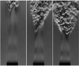
The schlieren visualisations of low-density jets from the nozzle with  $L/D = 175$ are shown in figure 3(a) and supplementary movie 1 available at https://doi.org/10.1017/jfm.2022.328. At low Reynolds numbers, the low-density jet is globally stable but convectively unstable. In this regime, the jet is relatively steady near the nozzle exit, whereas some oscillations are seen far from the nozzle exit (supplementary movie 1). The width of the jet remains almost constant, and the transition to turbulence or break down occurs far from the nozzle exit ( $x >12$). With an increase in Reynolds number, there is a qualitative change in the behaviour of low-density jets, i.e. the jets become globally unstable. The globally unstable low-density jet shows regular vortex formation from the nozzle exit. This vortex travels downstream for some distance and breaks down abruptly, resulting in a considerable jet spread after the breakdown. This breakdown location moves towards the nozzle exit with an increase in Reynolds number.

Figure 3. Schlieren visualisation of global oscillations in helium jet ( $S=0.138$) from the nozzle with (a) $L/D = 175$ and (b) $L/D = 8$.
The schlieren images of low-density jets from the nozzle with  $L/D = 8$ are shown in figure 3(b) and supplementary movie 2 to understand the qualitative differences with the low-density jets with $D/\theta _0 = 15$. Low-density jets with top-hat velocity profiles have lower critical Reynolds numbers, intense oscillations, a smaller transition/breakdown distance and a higher jet spread than low-density jets with $D/\theta _0 = 15$. The shorter breakdown distance indicates that the growth rate of disturbance is higher for globally unstable low-density jets with top-hat velocity profiles than low-density jets with $D/\theta _0 = 15$. One of the reasons for a higher jet spread in low-density jets with top-hat velocity profiles is the occurrence of side jets which can be seen in supplementary movie 2. No side jets are observed in the globally unstable low-density jets with $D/\theta _0=15$ for the range of parameters ( $Re$ and $S$) studied in the present experiments.
The frequency spectra from the time series of hotwire measurements show a sharp narrowband peak after the onset of oscillations (figure 4). The dominant fundamental frequency remains constant with the downstream distance from the jet inlet to the breakdown location, confirming the global oscillation. The frequency spectra from the low-density jets with top-hat velocity profiles show subharmonics, indicative of vortex pairing (Kyle & Sreenivasan Reference Kyle and Sreenivasan1993), for some parameter range (figure 4b). There are no subharmonics observed for the globally unstable low-density jets with  $D/\theta _0=15$. The increments of Reynolds number used in the present experiments are higher than the hysteresis Reynolds number range or the bistable region observed in the recent experiments of Zhu et al. (Reference Zhu, Gupta and Li2017). Due to this, it is impossible to identify the Hopf bifurcation type (supercritical or subcritical) in low-density jets from the present experiments.

Figure 4. Frequency spectrum of the time series from the hotwire anemometer located at  $x = 1.0$ and $r=0$ for (a) $Re= 3654$, $S = 0.138$ and $D/\theta _0 = 15$, and (b) $Re= 2357$, $S = 0.138$ and $D/\theta _0 = 26.7$.
From the schlieren visualisation (figure 3 and supplementary movies 1 and 2), it can be concluded that the shape of the globally unstable mode is axisymmetric. If a low-density jet is globally unstable then an axisymmetric global oscillation is observed for all the cases studied in the experiments, irrespective of  $S$,
$S$,  $Re$ and $D/\theta _0$. The same results are observed in the spatiotemporal stability analysis in the present study (§§ 5.2 and 5.3).
The present results are consistent with the previous experimental studies on low-density jets with inlet velocity profiles far from parabolic, exhibiting axisymmetric global oscillations (Monkewitz & Sohn Reference Monkewitz and Sohn1988; Kyle & Sreenivasan Reference Kyle and Sreenivasan1993; Hallberg & Strykowski Reference Hallberg and Strykowski2006). However, the current experimental results for the low-density jets with  $D/\theta _0 = 15$ differ from the stability results of Coenen et al. (Reference Coenen, Sevilla and Sánchez2008). They predicted that the helical mode of global oscillation might occur in low-density jets with near parabolic velocity profiles ( $D/\theta _0 \approx 15$) for $S<0.5$ from the spatiotemporal instability analysis. The possible reasons for the discrepancy of Coenen et al. (Reference Coenen, Sevilla and Sánchez2008) results are discussed in § 5.5.
4.2.1. Onset and frequency of global oscillations
The variation of Strouhal number ( $St = f^* D/U^*_j$) with Reynolds number ( $Re$) and $D/\theta _0$ are shown in figures 5(a) and 5(b), respectively. Note that for nozzles with $L/D = 8$ and 36, $D/\theta _0$ increases with an increase in Reynolds number for a given $L/D$. The nozzle with $L/D = 175$ has $D/\theta _0 = 15$ for the range of Reynolds number studied in the present experiments.

Figure 5. The variation of global oscillation Strouhal number ( $St$) with (a) Reynolds number and (b) nozzle exit momentum thickness for various density ratios.
The Strouhal number increases with an increase in density ratio, irrespective of Reynolds number and  $D/\theta _0$. For a given Reynolds number, the Strouhal number is a function of $D/\theta _0$ (figure 5a). The Strouhal number of the low-density jet with $D/\theta _0 = 15$ ( $L/D = 175$) is almost independent of the Reynolds number. For a given density ratio, the Strouhal number increases with an increase in $D/\theta _0$, irrespective of the Reynolds number (figure 5b). These results indicate that $D/\theta _0$ and density ratio significantly influence the Strouhal number and the effect of Reynolds number on Strouhal number seems to be small in the range of parameters studied in the experiments. Figure 6 shows the onset of global oscillations in the $Re-D/\theta _0$ space for different density ratios. For a given density ratio, the critical Reynolds number increases with a decrease in $D/\theta _0$. The critical Reynolds number increases with an increase in density ratio for a constant $D/\theta _0$, and the critical density ratio increases with an increase in $D/\theta _0$ for a constant Reynolds number. The critical Reynolds numbers from the present experiments reasonably match the experimental results of Hallberg & Strykowski (Reference Hallberg and Strykowski2006). The above results indicate that the higher disturbance levels in the present experiments are not significant enough to influence the critical Reynolds number of low-density jets.

Figure 6. The onset of global oscillations in low-density jets. The jets are globally unstable for parameters right side of the critical points.
The Strouhal number of the axisymmetric mode predicted by the linear bi-global stability analysis (Coenen et al. Reference Coenen, Lesshafft, Garnaud and Sevilla2017) and the DNS (Lendínez Reference Lendínez2018) for the low-density jet with  $D/\theta _0 = 15$ are 0.136 and 0.145, respectively, which are comparable with the experimental results ( $St\approx 0.138$). The critical Reynolds number predicted from the linear global stability analysis ( $Re \approx 3370$) and the DNS ( $Re \approx 2300$) is higher and lower than the experimental results ( $Re = 2844$), respectively. Numerical simulation of an isothermal helium jet with $D/\theta _0 = 15$ using an unsteady axisymmetric laminar solver at $Re = 1600$ by Satti & Agrawal (Reference Satti and Agrawal2006) shows global oscillation. This Reynolds number is much lower than the critical Reynolds number from the experiments. It is expected that the critical Reynolds number from the experiment might be lower than the linear stability analysis and numerical simulations due to the presence of noise in the experiments, which can prematurely trigger the transition from a globally stable state to a globally unstable state. The reason for predicting the lower critical Reynolds number from the numerical simulations (Satti & Agrawal Reference Satti and Agrawal2006; Lendínez Reference Lendínez2018) compared with the experimental results for low-density jets with $D/\theta _0=15$ is not clear. Further studies are required to understand this behaviour which is beyond the scope of this paper.
4.2.2. Comparison with scaling laws
In this section the experimental results are compared with scaling laws derived from theoretical and experimental studies. In the nonlinear spatiotemporal theory, if the base flow is nonlinearly absolute, any impulse perturbation in the flow creates a front that moves towards the nozzle exit and forms a nonlinear global mode. According to the theory, the healing length, which is defined as the distance for the perturbation amplitude of the nonlinear global mode to reach 99 % of the saturation amplitude, scales with  $(Re-Re_c)^{-0.5}$ which is derived from the Ginzburg–Landau amplitude equation (Couairon & Chomaz Reference Couairon and Chomaz1999). This scaling is valid for a nonlinear global mode in parallel and weakly non-parallel flows (Chomaz Reference Chomaz2004, Reference Chomaz2005). Experimental (Goujon-Durand, Jenffer & Wesfreid Reference Goujon-Durand, Jenffer and Wesfreid1994; Zielinska & Wesfreid Reference Zielinska and Wesfreid1995; Wesfreid, Goujon-Durand & Zielinska Reference Wesfreid, Goujon-Durand and Zielinska1996) and numerical studies (Chomaz Reference Chomaz2004) demonstrated that the healing length of a nonlinear global mode in a weakly non-parallel wake flow follows this scaling.
From the DNS studies of low-density jets (Nichols et al. Reference Nichols, Schmid and Riley2007), it can be observed that the vorticity fluctuations initially grow exponentially and then saturate after some distance. The jet spread increases dramatically approximately after this location. So, the jet breakdown location can be considered where the disturbance amplitude of a nonlinear global mode saturates. The jet breakdown distance or healing length in a globally unstable low-density jet is defined as the distance from the nozzle exit to the location where the jet spread increases suddenly (figure 3). In the present study the jet breakdown location is measured from schlieren images. The axial location where the cross-sectional (along  $y$-axis) mean pixel intensity of the average schlieren image starts increasing is considered as the jet breakdown location. This jet breakdown distance or healing length decreases with an increase in Reynolds number and scales with $(Re-Re_c)^{-0.5}$ for low-density jets from the nozzle with $L/D = 8$ and $L/D = 175$ (figure 7a). Even though the proportional constant is a function of nozzle inlet conditions, this scaling will be useful for predicting the jet breakdown distance. This result extends the validity of the Ginzburg–Landau model, from which this scaling law is derived, to the low-density jet, which has a nonlinear global mode in the weakly non-parallel flow.

Figure 7. Comparison of experimental results with scaling laws for (a) the variation of healing length (Couairon & Chomaz Reference Couairon and Chomaz1999), (b) the frequency of global oscillations (Hallberg & Strykowski Reference Hallberg and Strykowski2006).
Hallberg & Strykowski (Reference Hallberg and Strykowski2006) proposed a universal scaling for global oscillation frequencies in low-density jets. The present experimental results are recast in the universal scaling form and are shown in figure 7(b). Except for the data from  $L/D=8$ with $S=0.138$, the scaling slope does not match the universal scaling. This may be explained by analysing the proportionality constants in the scaling law, which are: (i) the relation between vortex speed and nozzle exit jet velocity, (ii) the relation between $D/\lambda$ ( $\lambda$ is the wavelength of the vortex) and $D/\theta _0$, and (iii) the relation between frequency and density ratio. A plausible reason for this deviation could be that the value of these constants may not be universal but depend on the detailed shape of velocity and density profiles near the nozzle exit, which depend on nozzle geometry details and inlet conditions at the nozzle exit.
5. Linear stability results
5.1. Base state profiles
Base profiles for the spatiotemporal stability analysis are obtained from solving the steady, laminar, axisymmetric version of governing equations (2.1)–(2.5) using ANSYS Fluent. The methodology used to obtain the base flow is similar to Bharadwaj & Das (Reference Bharadwaj and Das2017). The governing equations are solved in an axisymmetric domain using a structured grid, and its schematic diagram with boundary conditions is shown in figure 8. The velocity profile with a given  $D/\theta _0$ and a constant mass fraction profile of helium corresponding to the density of the helium–air mixture are imposed at the inlet. The velocity profile for the inlet is selected from the axisymmetric pipe profiles, which are obtained from solving the laminar incompressible boundary layer equations inside an axisymmetric pipe (Joshi & Vinoth Reference Joshi and Vinoth2018). The pressure outlet condition, which extrapolates the interior's flow variables, is specified at far-field boundaries and the domain exit. No-slip is specified on the nozzle wall, and the axis of symmetry is imposed on the axis. Note that the nozzle/tube has zero wall thickness in the simulations. The gravity force is acting opposite to the flow direction. The viscosity of the helium–air mixture is computed using the relation given by Wilke (Reference Wilke1950), and the mass diffusive coefficient between air and helium is assumed to be a constant. The steady base profiles are computed using a pressure-based coupled solver with the pseudo-transient method. The second-order upwind scheme is used for the discretization of pressure and momentum terms. These equations are solved until the residual drops below $10^{-6}$.

Figure 8. Schematic diagram of the computational domain with boundary conditions used for simulating base flows.
The domain size of ( $30D \times 6D$) ( $x$ and $r$ directions) is used in the present study. The number of nodes used before and after the nozzle exit are ( $210 \times 166$) and ( $262 \times 216$), respectively. The domain size and the number of nodes, which are clustered near the nozzle exit, are selected based on convergence studies. The base flow solution methodology is validated with the laminar plume results of Bharadwaj & Das (Reference Bharadwaj and Das2017). The laminar base state profiles (velocity and density) of low-density jets with $D/\theta _0 = 15, Re=3600, S=0.138$, and $D/\theta _0 = 32.2, Re=3520, S=0.338$ are shown in figure 9. In laminar flows the main source for the jet spread is molecular diffusion, due to which the laminar profiles (velocity and density) evolve slowly along the flow direction. The spread of the density profiles is relatively higher compared with the velocity profiles. These results are consistent with the base flows reported in Coenen et al. (Reference Coenen, Lesshafft, Garnaud and Sevilla2017).

Figure 9. Base flow velocity (a,c) and density profiles (b,d) at various streamwise locations for  $Re=3600, D/\theta _0=15$ and $S=0.138$ (a,b), and $Re=3520, D/\theta _0 = 32.2$ and $S=0.338$ (c,d).
5.2. Spatiotemporal stability results near the nozzle exit
The velocity and density profiles from the numerical simulations are used as base states for the spatiotemporal stability analysis. Figure 10 shows the solution of the dispersion relation in the complex  $k$ plane for $S=0.138$, $D/\theta _0 =15$ and $Re =3600$ at the location very near the nozzle exit ( $x = 0.01$). Each line in the figure is a solution to the spatial eigenvalue problem for a given $\omega _i$ with varying $\omega _r$. Spatial branches are classified based on the location of the entire spatial branch for $\omega _i > \omega _{i,max}$, where $\omega _{i,max}$ is the maximum growth rate in temporal stability analysis. The branches are classified as $k^+$ and $k^-$ if they are located above and below the $k_r$-axis. In the present study, a single $k^+$ branch is observed along with many $k^-$ branches. Even though many saddles are formed near the $-k_i$-axis, only the first two saddles ( $S_1$ and $S_2$) and three spatial branches $k^+, k_1^-$ and $k_2^-$ are shown in figure 10.

Figure 10. Saddle points in the complex  $k$-plane of (a) axisymmetric mode ( $m=0$) and (b) helical mode ( $m=1$), for $S=0.138$, $Re = 3600$, $D/\theta _0 = 15$ and $x = 0.01$.
Initially, all the spatial branches are well separated for a large  $\omega _i$. With a decrease in $\omega _i$, the $k^+$ branch pinches with $k_1^-$ to form saddle $S_1$ (see figure 10a). For a further decrease in $\omega _i$, the merged $k_1^-$ branch pinches with $k_2^-$ to form saddle $S_2$. According to the Briggs–Bers criterion, the valid saddle forms by pinching $k^+$ and $k^-$ spatial branches (Huerre & Monkewitz Reference Huerre and Monkewitz1990; Huerre & Rossi Reference Huerre and Rossi1998). Based on the above criteria, $S_1$ is the only valid saddle, and other saddles which occur below, including $S_2$ are invalid. The absolute growth rate of $S_1$ is positive ( $\omega _{0,i} > 0$), i.e. the axisymmetric mode is absolutely unstable. In the case of helical mode ( $m=1$), the formation of $S_1$ and $S_2$ show similar behaviour in the complex $k$ plane compared with the axisymmetric mode, i.e. $S_1$ is the valid saddle (figure 10b). The main difference is that the helical mode $S_1$ is convectively unstable ( $\omega _{0,i} < 0$). Based on the above results, it can be concluded that the spatiotemporal behaviour of the jet at this location is dominated by the axisymmetric mode, which is absolutely unstable. Similar results are observed for all low-density jets at this location irrespective of $S, Re$ and $D/\theta _0$, i.e. if the low-density jet is absolutely unstable then the dominant mode is axisymmetric.
The eigenfunctions corresponding to  $S_1$ of the axisymmetric mode are shown in figure 11. The pressure eigenfunction ( $\hat {p}$) has a maximum value at the centreline and decreases gradually with an increase in the radial direction, whereas the streamwise velocity eigenfunction ( $\hat {u}_x$) has a local peak in the shear layer with a non-zero value at the jet centreline. The behaviour of these eigenfunctions is consistent with the jet column mode reported in the literature (Jendoubi & Strykowski Reference Jendoubi and Strykowski1994; Srinivasan et al. Reference Srinivasan, Hallberg and Strykowski2010; Demange, Chazot & Pinna Reference Demange, Chazot and Pinna2020a). Similar results are observed for all absolutely unstable low-density jets, irrespective of $S, Re$ and $D/\theta _0$. Lesshafft & Huerre (Reference Lesshafft and Huerre2007) reported that the nature of the dominant saddle's eigenfunction changes with an increase in velocity profile momentum thickness of low-density jets. The eigenfunction of the dominant saddle of thin shear layer jets shows the jet column mode, and in the case of thick shear layer jets, it is the mixed mode (combination of jet column mode and shear layer mode). This result contrasts with the present study, where the nature of the mode (jet column mode) is the same irrespective of $D/\theta _0$. The main difference is that the present study used profiles from the numerical simulations as a base state, whereas they used base states from solving the boundary layer equations with the model velocity and density profiles in the inlet (table 1).

Figure 11. Eigenfunctions (axial velocity  $\hat {u}_x$, radial velocity $\hat {u}_r$, density $\hat {\rho }$ and pressure $\hat {p}$) of the dominant axisymmetric mode ( $S_1$ saddle) for $S=0.138$, $Re = 3600$, $D/\theta _0 = 15$ and $x = 0.01$.
5.3. Streamwise variation of stability results
In weakly developing flows, where the instability wavelength ( $\lambda$) is much less than the length scale of the base flow ( $L \sim [(1/\theta )({\rm d}\theta /{{\rm d}\kern0.7pt x})]^{-1}$), there exists a close relationship between the local stability characteristics from different streamwise locations ( $x$) and the global dynamics of the flow (Huerre & Monkewitz Reference Huerre and Monkewitz1990; Huerre & Rossi Reference Huerre and Rossi1998). In the present study the ratio $\epsilon _1 = \lambda /L$ is high near the nozzle exit ( $\epsilon _1 \sim 0.7$ for $D/\theta _0 =30$ and $\epsilon _1 \sim 0.1$ for $D/\theta _0 =15$) and decreases away from the nozzle exit. The value of $\epsilon _1$ decreases with a decrease in $D/\theta _0$. Even though the base flow variation near the nozzle exit is not weakly parallel for high $D/\theta _0$, the local spatiotemporal stability studies on low-density jets, which is similar to the present study, favourably predict the global dynamics observed in experiments (Coenen & Sevilla Reference Coenen and Sevilla2012). In addition to that, the studies on the wake of a cylinder (Pier Reference Pier2002) and sphere (Pier Reference Pier2008) have also shown favourable results, even the base flow variation is not weakly non-parallel near the solid body. In order to obtain the global stability characteristics from the local stability characteristics, the streamwise evolution of stability is discussed in this section.
The absolute growth rate ( $\omega _{0,i}$) variation of the axisymmetric ( $m=0$) and helical mode ( $m=1$) with the streamwise direction ( $x$) are shown in figures 12(a) and 12(b), respectively, for $S=0.138$ and $D/\theta _0=15$. These results are obtained by tracking $S_1$ along the streamwise direction using the three-point method. It is observed that the nature of $S_1$ is the jet column mode, irrespective of streamwise distance. The absolute growth rate shows a non-monotonous behaviour with the streamwise distance, i.e. the absolute growth rate curve has a maximum. The location of the maximum growth rate occurs near the nozzle exit, which is almost independent of Reynolds number (figure 12a,b). Note that there is a discontinuity in the absolute growth rate curve slope near the nozzle exit ( $x \approx 0.02$). The reason for the discontinuity is not known as there is no appreciable difference in the profiles (velocity and density) near the location where the discontinuity is observed. Similar behaviour, i.e. discontinuity in absolute growth rate curve near the nozzle exit, can also be seen in figure 3 of Coenen & Sevilla (Reference Coenen and Sevilla2012).

Figure 12. Streamwise variation ( $x$) of the absolute growth rate ( $\omega _{0,i}$) of (a) axisymmetric mode ( $m=0$) and (b) helical mode ( $m=1$) for $S=0.138$ and $D/\theta _0 = 15$ at different Reynolds number.
At a low Reynolds number ( $Re = 1900$), the absolute growth rate is negative for all streamwise locations (figure 12a). With an increase in Reynolds number, the absolute growth curve first becomes marginally unstable ( $\omega _{0,i}=0$) at $x \approx 0.2$, and then a pocket of the absolutely unstable ( $\omega _{0,i}>0$) region occurs, i.e. the absolutely unstable region is bounded by the convectively unstable region in both upstream and downstream directions. For a further increase in Reynolds number, the region of the absolutely unstable region grows, and the upstream portion of the pocket of the absolutely unstable region reaches the nozzle exit. Subsequently, the length of the absolute region ( $l_{abs} =x_{ac}$; $x_{ac}$ is the location where the instability changes from absolute to convective) bounded by the nozzle exit increases with an increase in Reynolds number. The absolute growth rate curves of the helical mode ( $m=1$) show similar non-monotonous behaviour, but they are convectively unstable (figure 12b). These results indicate that the axisymmetric mode is the dominant absolutely unstable mode for $S=0.138$ and $D/\theta _0 =15$, which may trigger a global axisymmetric oscillation.
Based on the stability results from the parameter space studied in this work, it can be concluded that irrespective of  $S, Re$ and $D/\theta _0$, the global oscillation in low-density jets shows an axisymmetric nature. As discussed in § 4.2, this result is consistent with the present experimental results. This result is also consistent with the experimental (Monkewitz et al. Reference Monkewitz, Bechert, Barsikow and Lehmann1990; Kyle & Sreenivasan Reference Kyle and Sreenivasan1993; Hallberg & Strykowski Reference Hallberg and Strykowski2006) and stability studies (Lesshafft et al. Reference Lesshafft, Huerre, Sagaut and Terracol2006, Reference Lesshafft, Huerre and Sagaut2007; Lesshafft & Huerre Reference Lesshafft and Huerre2007; Nichols et al. Reference Nichols, Schmid and Riley2007; Coenen et al. Reference Coenen, Sevilla and Sánchez2008; Coenen & Sevilla Reference Coenen and Sevilla2012) on low-density jets with velocity profiles far from parabolic, which show global axisymmetric oscillations. Stability studies by Coenen et al. (Reference Coenen, Sevilla and Sánchez2008) predicted that low-density jets with near parabolic velocity profiles might show a helical mode of global oscillations, which is different from the present stability and experimental results.
The evolution of the axisymmetric absolute growth rate with the streamwise distance of  $S=0.338$ and $D/\theta _0 = 31.3$ for various Reynolds number is shown in figure 13(a). The absolute growth rate shows a monotonous decrease with the streamwise distance. With an increase in Reynolds number, the absolute growth rate at the nozzle exit first become marginally unstable ( $\omega _{0,i}^0 = \omega _{0,i}(x=0)=0$) and then, the length of the absolutely unstable region bounded by the nozzle exit ( $x_{ac}$) increases. Figure 13(b) shows the effect of density ratio on the axisymmetric absolute growth rate variation with the streamwise distance for $Re=4000$ and $D/\theta _0 = 15$. The shape/variation of the absolute growth rate curve with the streamwise direction depends on the density ratio. The absolute growth rate curve shows a non-monotonous behaviour for $S = 0.138$ and $0.15$, whereas it shows a monotonous decrease with the streamwise direction for $S = 0.2$. Detailed analysis of base profiles, such as the inflection point in velocity profiles, the slope of the density profile gradient near to the velocity inflection point, the distance between the inflection point in velocity and density profiles (Raynal et al. Reference Raynal, Harion, Favre-Marinet and Binder1996; Lesshafft & Marquet Reference Lesshafft and Marquet2010; Demange et al. Reference Demange, Chazot and Pinna2020a), do not reveal possible reasons for the non-monotonous behaviour of absolute growth curves. Nevertheless, from the stability results, it can be summarised that the non-monotonous behaviour of the absolute growth rate is observed for density ratio $S\lesssim 0.16$, irrespective of $D/\theta _0$.

Figure 13. Streamwise variation ( $x$) of the axisymmetric absolute growth rate ( $\omega _{0,i}$). (a) Effect of Reynolds number for $S=0.338$ and $D/\theta _0 = 31.3$, and (b) effect of density ratio for $Re=4000$ and $D/\theta _0 = 15$.
A monotonous decrease of the axisymmetric absolute growth rate curves with the maximum at the nozzle exit was reported for low-density jets where the base flow profiles were obtained from solving the boundary layer equations with a synthetic velocity and density profile at the nozzle exit (Lesshafft et al. Reference Lesshafft, Huerre, Sagaut and Terracol2005, Reference Lesshafft, Huerre, Sagaut and Terracol2006, Reference Lesshafft, Huerre and Sagaut2007). Studies that used the boundary layer equations to obtain the inlet profiles and its evolution with streamwise direction (base flow profiles) reported non-monotonous absolute growth rate curves for  $m=0$ only in low-density jets with thin shear layers (Coenen et al. Reference Coenen, Sevilla and Sánchez2008; Coenen & Sevilla Reference Coenen and Sevilla2012), whereas the absolute growth rate curves of $m=1$ show a monotonous decrease, irrespective of $D/\theta _0$ (Coenen et al. Reference Coenen, Sevilla and Sánchez2008). In summary, studies that did not use actual velocity and density profiles as the base flow show a different nature of absolute growth rate curves compared with the present study. From these results, it can be inferred that the nature of the absolute growth rate curve, whether it is monotonous or non-monotonous, depends on the shape of base flow velocity and density profiles.
All the stability results presented in this paper are obtained using the linearised stability equations with constant viscosity and negligible buoyancy. Note that apart from appearing in the stability equations, the transport property (viscosity) and buoyancy also affect the base flow profiles, which indirectly influence the stability characteristics of the jet. In the present study all the base flow simulations included the effect of variable viscosity and buoyancy. The inclusion of variable viscosity terms in the stability equations for a given base state has a very less stabilizing effect than the constant viscosity case, and there is almost no effect on the absolute growth rate by including the buoyancy term in the stability equations (not shown). The above results give justification for neglecting the effect of variable viscosity and buoyancy in the stability computation reported in this paper.
5.4. Comparison with experimental results
This section compares local spatiotemporal stability results with the experimental results to understand the selection criteria for destabilising a nonlinear global mode. The effect of Reynolds number on the absolute growth rate at the nozzle exit,  $\omega _{0,i}^0$, and the maximum absolute growth rate, $\omega _{0,i}^{max}$, of the axisymmetric mode, is shown in figure 14(a) for $S = 0.138$ and $D/\theta _0=15$. The corresponding experimental critical condition is shown in the figure as a dashed line. The maximum absolute growth rate is marginally unstable ( $\omega _{0,i}^{max}=0$) at $Re \approx 2140$, and a pocket of the absolutely unstable region appears at $2140 \lesssim Re \lesssim 2350$, whereas the absolute growth rate at the nozzle exit becomes marginally unstable at $Re \approx 2350$ (figure 14a). The experimental critical Reynolds number ( $Re \approx 2844$) is higher than the Reynolds number corresponding to the marginal stability of both $\omega _{0,i}^0$ and $\omega _{0,i}^{max}$. From the above results, it can be inferred that the nonlinear global mode is destabilised after a minimum length of the absolutely unstable region $l_{abs}$ (table 2). Figure 14(b) shows the effect of density ratio on the axisymmetric absolute growth rate at the nozzle exit ( $\omega _{0,i}^0$) for $Re=4000$ and $D/\theta =15$ along with the experimental critical density ratio. The density ratio ( $S\approx 0.15$) required to excite the global mode in experiments is lower than the density ratio ( $S\approx 0.2$) corresponding to the marginal absolute instability at the nozzle exit ( $\omega _{0,i}^0=0$). Similar results, i.e. the requirement of a minimum length of the absolutely unstable region to sustain the nonlinear global mode, are observed for all the cases studied in the present work, irrespective of whether the absolutely unstable region is bounded by the nozzle exit or the occurrence of a pocket of the absolutely unstable region (table 2).

Figure 14. (a) The variation of the absolute growth rate of the axisymmetric mode at the nozzle exit,  $\omega _{0,i}^0$, and maximum absolute growth rate, $\omega _{0,i}^{max}$, with Reynolds number for $S=0.138$ and $D/\theta _0 = 15$, and (b) the variation of the absolute growth rate of the axisymmetric mode at the nozzle exit, $\omega _{0,i}^0$, with density ratio for $Re=4000$ and $D/\theta _0 = 15$. The dashed line denotes the experimental critical condition.
Table 2. Comparison of spatiotemporal stability parameters (length of the absolutely unstable region,  $l_{abs}$; absolute wavelength at the nozzle exit, $\lambda _0$; the constant ( $C$) in the criterion proposed by Chomaz, Huerre & Redekopp Reference Chomaz, Huerre and Redekopp1988) at the experimental critical conditions ( $S, D/\theta _0$ and $Re$) along with Reynolds number ( $Re_0$) corresponds to the marginal absolute growth rate at the nozzle exit.
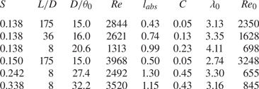
Contrary to the results in the literature (Lesshafft et al. Reference Lesshafft, Huerre, Sagaut and Terracol2006), the occurrence of a pocket of an absolutely unstable region does not destabilise a nonlinear global mode. The present results are consistent with the studies where the nozzle exit bounds the absolutely unstable region. In this scenario, a minimum length of the absolutely unstable region is required to trigger the nonlinear global mode (Pier et al. Reference Pier, Huerre, Chomaz and Couairon1998; Pier & Huerre Reference Pier and Huerre2001; Lesshafft et al. Reference Lesshafft, Huerre, Sagaut and Terracol2006; Coenen & Sevilla Reference Coenen and Sevilla2012). Compared with Lesshafft et al. (Reference Lesshafft, Huerre, Sagaut and Terracol2006) results, the pocket of the absolutely unstable region observed in the present study is very small and occurred near the nozzle exit. In addition, the pocket of an absolutely unstable region is observed only for a small range of Reynolds numbers. The present results suggest that the size and location of a pocket of an absolutely unstable region and the range of Reynolds number of its occurrence are also essential factors to excite the global mode. It can be concluded that the occurrence of a pocket of an absolutely unstable region itself cannot sustain the global mode if its characteristics are similar to the present study. A similar conclusion can be inferred from the results of Coenen et al. (Reference Coenen, Lesshafft, Garnaud and Sevilla2017). In their study, the global stability analysis predicted that the critical/marginal stability condition occurs at  $Re_m \approx 380$ for $S=0.143$ and $D/\theta _0 =24.3$. For the corresponding conditions ( $S=0.143$ and $D/\theta _0 =24.3$), a pocket of an absolutely unstable region might have occurred in the spatiotemporal stability analysis much below the critical Reynolds number predicted by the global stability analysis (refer to figures 9 and 10 of Coenen et al. Reference Coenen, Lesshafft, Garnaud and Sevilla2017).
The literature reported two different conditions for the minimum length requirement of an absolutely unstable region to trigger the nonlinear global mode. Based on the studies using the Ginzburg–Landau equation, the minimum absolutely unstable region ( $l_{abs}$) required to trigger the nonlinear global mode is given as $l_{abs} = C/\sqrt {\sigma _0}$, where ${\sigma _0} = \omega _{0,i}^0$ and $C$ is a constant (Chomaz et al. Reference Chomaz, Huerre and Redekopp1988; Couairon & Chomaz Reference Couairon and Chomaz1999). In low-density jets, Coenen & Sevilla (Reference Coenen and Sevilla2012) reported that the value of $C$ is not a constant but a function of density ratio ( $C=0.85$ for $S=0.14$ and $C=0.41$ for $S=0.5$). These values are different from the value ( $C=3.57$) obtained from the Ginzburg–Landau equation (Chomaz et al. Reference Chomaz, Huerre and Redekopp1988). The present results also show that the values of $C$ are not constant ( $C \approx 0.05$ for $D/\theta _0 =15$ and $0.13 \lesssim C \lesssim 0.45$ for higher $D/\theta _0$) and closer to Coenen & Sevilla (Reference Coenen and Sevilla2012) (table 2).
The second condition is that the minimum length of the absolutely unstable region should be of the order of one absolute wavelength at the nozzle exit,  $\lambda _0 = 2 {\rm \pi}/k_{0,r}(x=0)$, where $k_{0,r}(x=0)$ is the real part of the absolutely unstable wavenumber at the nozzle exit. This phenomenological criterion was proposed by Lesshafft et al. (Reference Lesshafft, Huerre, Sagaut and Terracol2006) based on numerical simulations of hot jets and confirmed by other studies (Bolaños-Jiménez et al. Reference Bolaños-Jiménez, Sevilla, Gutiérrez-Montes, Sanmiguel-Rojas and Martínez- Bazán2011; Demange et al. Reference Demange, Pinna, Qadri and Juniper2020b). In the present study the length of the absolutely unstable region ( $l_{abs}$) required to sustain the global mode is much smaller than the absolute wavelength at the nozzle exit ( $\lambda _0$) (table 2).
According to the stability theory, the frequency of a nonlinear global mode at the critical conditions is equal to the absolute frequency at the nozzle exit (Chomaz Reference Chomaz2005). The absolute Strouhal numbers at the nozzle exit,  $St_0$ ( $St_0 =\omega _{0,r}(x=0)/2 {\rm \pi}$), corresponding to the experimental critical conditions are compared with the experimental Strouhal numbers, $St$, in table 3. The relative differences between these Strouhal numbers are in the range of 11 %–16 %, which are similar to the results reported by Lesshafft et al. (Reference Lesshafft, Huerre, Sagaut and Terracol2005) and Coenen & Sevilla (Reference Coenen and Sevilla2012). Sensitivity analysis from the global stability revealed that the region near the nozzle exit has a strong influence on the growth rate of a global mode (Coenen et al. Reference Coenen, Lesshafft, Garnaud and Sevilla2017). In the present study the nozzle lip thickness was not included in the base flow simulations, which might have caused a subtle difference in the base flow profiles near the nozzle exit, and this might be a possible reason for the deviation observed in the marginal frequency of global oscillations compared with experiments. In summary, it can be concluded that the local spatiotemporal stability analysis can reasonably predict the frequency of global oscillations at critical conditions using the absolute frequency at the nozzle exit.
Table 3. Global frequencies from experiments ( $St$), the absolute frequency at the nozzle exit ( $St_0$) corresponds to the experimental critical conditions and the relative difference between them.

We conclude this section with a discussion regarding the possible implications of high level disturbances at the nozzle exit on low-density experimental results. Global frequency response studies on low-density jets with  $D/\theta _0=15$ by Lendínez (Reference Lendínez2018) demonstrated that $m=1$ has the largest gain for both optimal and uniform forcing conditions compared with $m=0$ and $m=2$. The difference between the gains of $m=1$ and $m=0$ increases with an increase in Reynolds number, and these differences reach at least ten orders near the critical Reynolds number (refer to figure 3.6 of Lendínez Reference Lendínez2018). The effect of the nozzle geometry and the region of forcing on the global frequency response also showed the same results, i.e. $m=1$ has higher gains than $m=0$ and $m=2$ for both optimal and uniform forcing. Based on the above results, we can plausibly conclude that the high disturbance level at the nozzle exit (possibly an axisymmetric nature of disturbance due to axisymmetric geometry) in the present experiments may not have affected the axisymmetric nature of the global oscillations in the low-density jets with $D/\theta _0 = 15$. The favourable comparison of the spatiotemporal stability results, which assumes disturbance is infinitesimal, with the low-density jet experiments with high disturbance levels at the nozzle exit showed that the axisymmetric nature of global oscillations in low-density jets with $D/\theta _0= 15$ is independent of disturbance level (at least up to the disturbance level in the present experiments).
5.5. Comparison with literature
This section compares the present results with the literature dealing with the stability analysis of low-density jets with near parabolic inlet velocity profiles (Coenen et al. Reference Coenen, Sevilla and Sánchez2008; Coenen & Sevilla Reference Coenen and Sevilla2012). These studies have used base flows from the boundary layer equations. In order to compare our results, we have also computed base flows from the boundary layer equations similar to Coenen et al. (Reference Coenen, Sevilla and Sánchez2008) and Coenen & Sevilla (Reference Coenen and Sevilla2012). Note that we have used the mean velocity at the nozzle exit ( $U^*_m$) and the nozzle radius ( $R$) as the characteristic velocity and characteristic length scale, respectively, in this section to compare the results with Coenen et al. (Reference Coenen, Sevilla and Sánchez2008) and Coenen & Sevilla (Reference Coenen and Sevilla2012). The Reynolds number based on the above reference scales is $Re_m = \rho ^*_j \, U^*_m \, R/\mu ^*_j$.
Coenen et al. (Reference Coenen, Sevilla and Sánchez2008) reported that low-density jets with near parabolic velocity profiles might exhibit a helical global oscillation based on the spatiotemporal stability analysis. This result is contrary to the present experimental and stability results. In this section we will explore the possible reasons for this discrepancy. Brief details about the methods used by Coenen et al. (Reference Coenen, Sevilla and Sánchez2008) for stability analysis are given here for understanding the discussion in this section. They have used a low-Mach-number version of the inviscid stability equation with pressure perturbation as a dependent variable. They have used two methods to compute the stability characteristics of low-density jets using the above equation. In the first method, the base flows (velocity and density) of low-density jets from the boundary layer equations are used with appropriate boundary conditions at the jet axis and far-field to compute absolute growth rates ( $\omega _{0,i}$) at different axial locations. This method is hereafter referred to as the ‘conventional method’ in this section.
In the second method, they have computed the stability characteristic of low-density jets at the jet inlet ( $x=0$) using nozzle exit profiles as given by
 \begin{equation} 0 \leqslant r \leqslant 1: \quad U = U(r), \ \rho = S \quad \text{and} \quad r > 1: \quad U = 0, \ \rho = 1. \end{equation}
These velocity profiles are obtained by solving the boundary layer equations inside an axisymmetric pipe. These profiles have zero velocity outside the nozzle radius ( $r > 1$) and discontinuity in the slope at the nozzle radius. The inlet jet density profiles are assumed to be a step function, i.e. the density is constant inside and outside the nozzle but changes suddenly at $r=1$. In order to overcome the difficulties of handling the profiles with slope discontinuity, they restricted the flow domain to $0\leqslant r \leqslant 1$ and applied the boundary conditions at $r=1$ from the analytical solution of the stability equation in the far-field. The second method used by Coenen et al. (Reference Coenen, Sevilla and Sánchez2008), which includes base state (velocity and density profiles with $0\leqslant r \leqslant 1$), stability equation (low-Mach-number inviscid stability equations), and boundary conditions from the analytical solution at $r=1$, is hereafter referred to as the ‘CSS08 method’ in this section.
Based on the conventional method, they have reported that  $\omega _{0,i}$ of $m=0$ and $m=1$ decreases monotonically with the axial distance for $D/\theta _0 \lessapprox 170$. In the above scenario, the marginal absolute instability condition is determined by $\omega _{0,i}$ at $x=0$, so it is sufficient to compute $\omega _{0,i}$ at $x=0$ to find critical conditions. They have reported that $\omega _{0,i}$ by the conventional method at $X \to 0$ ( $X=x^*/(R \, Re_{m})$) matches with $\omega _{0,i}$ from the CSS08 method and, as a consequence, have reported most of the results based on $\omega _{0,i}$ of the CSS08 method including the dominance of a helical mode over an axisymmetric mode in low-density jets with near parabolic velocity profiles.
It is known from the analytical work of Kambe (Reference Kambe1969) that the axisymmetric mode is neutrally stable in the inviscid temporal stability and stable in the viscous temporal stability for constant density jets with a parabolic velocity profile surrounded by a fluid at rest. The CSS08 method is similar to the method used by Kambe (Reference Kambe1969) in terms of the velocity profile and the application of the boundary conditions. The result of Kambe (Reference Kambe1969) promotes the question of the efficacy of the CSS08 method for low-density jets with near parabolic velocity profiles because the maximum temporal growth rate bounds the absolute growth rate.
In order to understand the validity of the CSS08 method for low-density jets with near parabolic velocity profiles, absolute growth rates from the conventional method at  $X=10^{-5}$ are compared with the CSS08 method for different $D/\theta _0$ (figure 15). The conventional method predicts that $\omega _{0,i}$ of $m=0$ is always higher than the $m=1$ for all $D/\theta _0$ including $D/\theta _0=15$. This result is consistent with the present viscous stability results using the numerical base flows (§ 5.3) and experimental results (§ 4.2), i.e. the global oscillation is axisymmetric for low-density jets with $D/\theta _0=15$. The absolute growth rate of $m=0$ from the CSS08 method is almost the same as the conventional method for large $D/\theta _0$. The difference between the absolute growth rates increases for a decrease in $D/\theta _0$, and this difference increases drastically when $D/\theta _0 \to 15$ (figure 15). Note that $\omega _{0,i}$ of $m=0$ by the CSS08 method reaches almost zero for $D/\theta _0 \to 15$, and it is less than $\omega _{0,i}$ of $m=1$. These results suggest that the global oscillation in low-density jets with $D/\theta _0=15$ might be helical, which is inconsistent with the results from the conventional method, the present stability analysis and the experiments.

Figure 15. Comparison of absolute growth rates from the conventional method at  $X=10^{-5}$ with the CSS08 method for $S=0.138$.
From the above results, it can be inferred that the main reason for the discrepancy is the assumption that  $\omega _{0,i}$ from the CSS08 method is equal to the $\omega _{0,i}$ from the conventional method at $X \to 0$. The present analysis clearly shows that this assumption is not valid for $D/\theta _0 \to 15$. The very small absolute growth rate of $m=0$ for $D/\theta _0 \to 15$ in the CSS08 method is due to the use of velocity and density profiles that lack inflection points and the implementation of boundary conditions at $r=1$. In summary, the CSS08 method may not be able to predict the results as observed in experiments for low-density jets with near parabolic velocity profiles (thick shear layer jets), but it may give qualitatively correct results, such as the most dominant mode for low-density jets with velocity profiles far from parabolic.
Coenen & Sevilla (Reference Coenen and Sevilla2012) studied the onset of global oscillations in low-density jets by viscous spatiotemporal stability analysis using base profiles obtained from the boundary layer equations. They reported that, for  $Re_m=1000 \ (Re=4000)$, the marginal absolute growth rate at the nozzle exit ( $\omega _{0,i}^0=0$) occurs at $S \approx 0.45$ for the jet with $D/\theta _0 = 15$ (figure 4b in Coenen & Sevilla Reference Coenen and Sevilla2012). This critical density ratio is much higher than the present stability result ( $S \approx 0.2$, see figure 14b) and the present experimental critical density ratio ( $S \approx 0.15$) for $Re_m=1000$. The difference between the current study and Coenen & Sevilla (Reference Coenen and Sevilla2012) is only in the base profiles. In order to understand the effect of base flow on viscous spatiotemporal stability results, the comparison of $\omega _{0,i}$ from viscous spatiotemporal stability using base profiles from the boundary layer equations and the Navier–Stokes equations (numerical simulation) is shown in figure 16(a) for the jet with $S=0.3, Re_m = 1000$ and $D/\theta _0=15$. The stability analysis using base profiles from the numerical simulation shows that the jet is convectively unstable for $m=0$ and $m=1$. In contrast, the stability analysis with boundary layer base profiles shows that the jet is absolutely unstable for $m=0$ near the nozzle exit and convectively unstable for $m=1$. The above results indicate that the difference between the profiles from the boundary layer equations and the numerical base profiles (Navier–Stokes equations) are significant enough to cause considerable change in the absolute growth rates, resulting in different critical density ratios for low-density jets with near parabolic velocity profiles.

Figure 16. (a) Absolute growth rate from the viscous spatiotemporal stability analysis using base profiles from the boundary layer equations (BL) and the Navier–Stokes equations (N–S), and (b) base density profiles from the boundary layer equation (BL) and the Navier–Stokes equations (N–S) for  $S=0.3, Re_m=1000$ and $D/\theta _0 = 15$.
This is an interesting result because it is expected that the profiles from the boundary layer equations and the Navier–Stokes equations are almost identical at these critical Reynolds numbers. The comparison of base profiles from the boundary layer equations and the Navier–Stokes equations reveals that the velocity profiles are almost the same (not shown), but density profiles show considerable differences in the near field (figure 16b). The density profiles from the Navier–Stokes equations show a higher spread than the density profiles from the boundary layer equations near the nozzle exit, and these differences decrease with an increase in the axial direction. Unlike the profiles from the boundary layer equations, the streamwise development of profiles from the Navier–Stokes equations does not scale (especially density profiles) with the Reynolds number near the nozzle exit, where the flow becomes absolutely unstable. Note that Coenen & Sevilla (Reference Coenen and Sevilla2012) results reasonably agree with Hallberg & Strykowski (Reference Hallberg and Strykowski2006) experiments for low-density jets with inlet profile far from parabolic. These results suggest that base profiles from boundary layer equations are sufficient for low-density jets with inlet velocity profiles far from parabolic. However, in the case of low-density jets with near parabolic inlet profiles, base profiles from the Navier–Stokes equations are required to predict the experimental critical conditions.
6. Summary and conclusion
Experimental and stability studies are carried out to study the global oscillations in low-density jets with parabolic velocity profiles. High-speed schlieren visualisations and hotwire measurements are carried out to capture low-density jets’ global and local dynamics. The spatiotemporal stability analysis is carried out using base flows from numerical simulations and the boundary layer equations.
Experimental results show that the global oscillations in low-density jets are axisymmetric irrespective of  $D/\theta _0$. This result is consistent with the present spatiotemporal stability analysis with base states from numerical simulations and the boundary layer equations. The present result is different from the prediction of spatiotemporal stability by Coenen et al. (Reference Coenen, Sevilla and Sánchez2008) which reported the global helical oscillations in low-density jets with near parabolic velocity profiles. The present study shows that the method used by Coenen et al. (Reference Coenen, Sevilla and Sánchez2008) (spatiotemporal stability analysis using profiles only inside the nozzle along with enforcing boundary conditions at the nozzle wall) may predict the experimental results for the jets with velocity profiles far from parabolic but not for the jets with near parabolic velocity profiles.
The breakdown location of the globally unstable low-density jet can be considered as the location where the disturbance amplitude of a nonlinear global mode saturates. The breakdown length or healing length of the globally unstable low-density jets scales with  $(Re-Re_c)^{-1/2}$. This is a significant result in the sense that apart from the wake flow, this is the other flow situation (to the best of the authors’ knowledge) where the healing length of a nonlinear mode in the weakly non-parallel flow satisfies the scaling derived from the Ginzburg–Landau model.
Unlike low-density jets with higher  $D/\theta _0$ where the side jets are observed for a specific range of parameters, no side jets are observed in globally unstable low-density jets with $D/\theta _0 = 15$. There are many hypotheses available in the literature for the formation of the side jets in a globally unstable jet, such as the secondary instability of a vortex ring similar to the Widnall instability (Monkewitz et al. Reference Monkewitz, Lehmann, Barsikow and Bechert1989; Monkewitz & Pfizenmaier Reference Monkewitz and Pfizenmaier1991), the formation of secondary streamwise vortices between primary vortex rings (Brancher, Chomaz & Huerre Reference Brancher, Chomaz and Huerre1994), the absolute secondary instability (Nichols et al. Reference Nichols, Chomaz, Schmid and Riley2008) and the secondary non-modal instability (Lopez-Zazueta, Fontane & Joly Reference Lopez-Zazueta, Fontane and Joly2016). However, the physical mechanism responsible for the side jets in a globally unstable jet is not clear. The low-density jet with $D/\theta _0 =15$ can be used to test the conjecture/hypothesis for the existence/non-existence of the side jets.
Contrary to the reported results (Lesshafft et al. Reference Lesshafft, Huerre, Sagaut and Terracol2006), the present study found that an occurrence of a pocket of the absolutely unstable region need not always destabilise a nonlinear global mode. The emergence of a nonlinear global mode possibly depends on the characteristics of the pocket of the absolutely unstable region, such as the size, location and the range of parameter (Reynolds number) it occurs. The present stability results show that there is a minimum length of the absolutely unstable region required to destabilise a nonlinear global mode, irrespective of whether the absolutely unstable region is bounded by the nozzle exit or the occurrence of a pocket of the absolutely unstable region for a specific range of parameters. At critical conditions, the required minimum length of the absolutely unstable region is much smaller than the absolute wavelength at the nozzle exit. These results are also different from the literature, where it is reported that the minimum length should be of the order of the absolute wavelength at the nozzle exit (Lesshafft et al. Reference Lesshafft, Huerre and Sagaut2007). The marginal absolute frequency at the nozzle exit favourably matches the experimental global frequency at the critical conditions. The present spatiotemporal stability results demonstrate that the base flows from the Navier–Stokes equations are required to predict the critical conditions observed in experiments for low-density jets with near parabolic velocity profiles.
Supplementary movies
Supplementary movies are available at https://doi.org/10.1017/jfm.2022.328.
Acknowledgements
The authors thank Dr M.P. Hallberg for clarifications and discussions regarding his JFM (2006) paper results. The authors thank H. Gupta for computing low-density jet base flows using the boundary layer equations and Dr M.T. Nair for his help to solve boundary layer equations for jet flows. S. S. Bangar, H.P. Gupta, A. Nyamagoudar are acknowledged for their contribution in stability and/or spatiotemporal studies in similar problems. U. S. Shrimali is acknowledged for his help in base flow simulations. The authors have acknowledged the help from Nasaruddeen N A (Aerodynamics lab) for conducting experiments and Prakash R S (Manufacturing lab) for fabrication of the experimental set-up. The authors would also like to thank the anonymous referees, whose comments helped shape the paper in its current form. A.B.N. is supported by a PhD fellowship from the Indian Institute of Space Science and Technology.
Funding
This research received no specific grant from any funding agency, commercial or not-for-profit sectors.
Declaration of interests
The authors report no conflict of interest.
Author contributions
B.R.V. conceptualised the research, A.B.N. designed and performed the experiments, A.D. developed stability codes and computed the stability results, and all authors involved in analysing the results and writing the paper.
Appendix A. Calibration of hotwire anemometry
In the present study the velocity profiles are measured using a single sensor normal hotwire probe (55P11). The hotwire anemometer responds to the velocity and density of the flow. Hence, to avoid the effects of density variation, the velocity profiles are measured in an air jet at the same Reynolds number. The hotwire probe is kept one diameter downstream of the nozzle exit at the jet centreline for calibration. The velocity profile at the nozzle exit is non-uniform due to the growth of the boundary layer inside the nozzle. Due to non-uniform velocity at the nozzle exit, the hotwire probe placed at the jet centreline measures velocity higher than the mean velocity measured from the mass flow rate. In order to obtain the correct velocity from the hotwire measurements, Johnstone et al. (Reference Johnstone, Uddin and Pollard2005) proposed an iterative procedure. This procedure corrects the velocity by comparing the actual volume flow rate with the volume flow rate from the velocity profile measured at the nozzle exit. The probe, which is kept close to the nozzle exit, measures the free shear layer due to an interaction between the jet and the surrounding in addition to the boundary layer from the nozzle exit. This may cause inaccuracies in the above procedure. In the present study the laminar velocity profile from a pipe flow is fitted to the measured velocity profile to eliminate the velocity due to free shear. The laminar velocity profiles are obtained by solving the boundary layer equations inside an axisymmetric pipe (Joshi & Vinoth Reference Joshi and Vinoth2018). The steps followed in the iterative procedure to calibrate the hotwire using non-uniform exit velocity profiles are given below.
(i) Measure the voltage at the jet centreline for each flow rate and compute the calibration velocity from the flow rate.
(ii) Obtain the calibration curve for the hotwire anemometer from the voltage and velocity data from (i), using a fourth-order polynomial curve fit.
(iii) For each calibration velocity, measure the velocity profile across the nozzle exit by measuring the voltage at each radial location across the nozzle exit using the calibration data from step (i).
(iv) Approximate the measured velocity profile at the nozzle exit from the collection of velocity profiles obtained from solving the boundary layer equations inside an axisymmetric pipe to eliminate the effect of the free shear layer.
(v) Calculate the volume-averaged mean flow velocity, $U_p$, by integrating the velocity profile obtained from (iv)
(vi) Calculate the correction factor
$c = U_f/U_p$, where $U_f$ is the actual mean flow velocity obtained from the flow meter.(vii) Multiply each calibration velocity in (i) by the corresponding correction factor to obtain the updated velocity.
(viii) Repeat steps (ii) to (vii) until results converge within the specified tolerance.


Appendix B. Linearized perturbation equations and boundary conditions
B.1. Linearized perturbation equations
Continuity equation,
 \begin{equation} \frac{{\rm d} \bar{\rho}}{{\rm d} r} \hat{u}_r + \frac{\bar{\rho}}{r} \hat{u}_r + \bar{\rho} \frac{{\rm d} \hat{u}_r}{{\rm d} r} + {\rm i} m \frac{\bar{\rho}}{r} \hat{u}_{\theta} + {\rm i} k \bar{\rho} \hat{u}_x + {\rm i} k U \hat{\rho} - {\rm i} \omega \hat{\rho} = 0. \end{equation}
 Radial ( $r$) momentum equation,
 \begin{align} &\frac{S}{\mu_{r} Re} \left[ \frac{4}{3} \frac{\bar{\mu}}{r^2} \hat{u}_r + \bar{\mu} \frac{m^2}{r^2} \hat{u}_r + \frac{2}{3 r} \frac{{\rm d} \bar{\mu}}{{\rm d} r} \hat{u}_r - \frac{4}{3} \bar{\mu} \frac{{\rm d}^2 \hat{u}_r}{{\rm d} r^2} + k^2 \bar{\mu} \hat{u}_r - \frac{4}{3} \frac{{\rm d} \bar{\mu}}{d r} \frac{{\rm d} \hat{u}_r}{d r} - \frac{4}{3r} \bar{\mu} \frac{{\rm d} \hat{u}_r}{{\rm d} r} \right] \nonumber\\ &\quad + {\rm i} k \bar{\rho} U \hat{u}_r - {\rm i} \bar{\rho} \omega \hat{u}_r + \frac{S}{\mu_{r} Re} \left[ \frac{7}{3} {\rm i} m \frac{\bar{\mu}}{r^2} \hat{u}_{\theta} + \frac{2}{3} \frac{{\rm i} m}{r} \frac{{\rm d} \bar{\mu}}{{\rm d} r} \hat{u}_{\theta} - \frac{1}{3} \frac{{\rm i} m \bar{\mu}}{r} \frac{{\rm d} \hat{u}_{\theta}}{{\rm d} r} \right] \nonumber\\ &\quad + \frac{S}{\mu_{r} Re} \left[ \frac{2}{3} {\rm i} k \frac{{\rm d} \bar{\mu}}{{\rm d} r} \hat{u}_x - \frac{1}{3} {\rm i} k \bar{\mu} \frac{{\rm d} \hat{u}_x}{{\rm d} r} \right] + \frac{{\rm d} \hat{p}}{{\rm d} r} + \frac{\bar{H} S}{\mu_{r} Re} \left[-{\rm i} k \frac{{\rm d} U}{{\rm d} r} \hat{\rho} \right] = 0. \end{align}
 Azimuthal ( $\theta$) momentum equation,
 \begin{align} &\frac{S}{\mu_{r} Re} \left[-\frac{{\rm i} m}{r} \frac{{\rm d} \bar{\mu}}{{\rm d} r} \hat{u}_r - \frac{7}{3} \frac{{\rm i} m}{r^2} \bar{\mu} \hat{u}_r - \frac{1}{3} \frac{{\rm i} m \bar{\mu}}{r} \frac{{\rm d} \hat{u}_r}{{\rm d} r} \right] + \frac{S}{\mu_{r} Re} \left[ \frac{4}{3} \frac{\bar{\mu} \, m^2}{r^2} \hat{u}_{\theta} + \frac{1}{r} \frac{{\rm d} \bar{\mu}}{{\rm d} r} \hat{u}_{\theta} \right.\nonumber\\ &\quad \left. + \frac{\bar{\mu}}{r^2} \hat{u}_{\theta} - \frac{\bar{\mu}}{r} \frac{{\rm d} \hat{u}_{\theta}}{{\rm d} r} - \bar{\mu} \frac{{\rm d}^2 \hat{u}_{\theta}}{{\rm d} r^2} - \frac{{\rm d} \bar{\mu}}{{\rm d} r} \frac{{\rm d} \hat{u}_{\theta}}{{\rm d} r} + k^2 \bar{\mu} \hat{u}_{\theta} \right] \nonumber\\ &\quad + {\rm i} k \bar{\rho} U \hat{u}_{\theta} + \frac{S}{\mu_{r} Re} \left[\frac{m k}{3 r}\bar{\mu} \hat{u}_x \right] + \frac{{\rm i} m}{r} \hat{p} - {\rm i} \bar{\rho} \omega \hat{u}_{\theta} = 0. \end{align}
 Axial ( $x$) momentum equation,
 \begin{align} &\bar{\rho} \frac{{\rm d} U}{{\rm d} r} \hat{u}_r + \frac{S}{\mu_{r} Re} \left[- {\rm i} k \frac{{\rm d} \bar{\mu}}{{\rm d} r} \hat{u}_r - \frac{{\rm i} k}{3} \bar{\mu} \frac{{\rm d} \hat{u}_r}{{\rm d} r} - \frac{{\rm i} k}{3 r} \bar{\mu} \hat{u}_r \right]+ \frac{S}{\mu_{r} Re} \left[\frac{1}{3} \frac{ m k \bar{\mu}}{r} \hat{u}_{\theta} \right] + {\rm i} k \bar{\rho} U \hat{u}_x \nonumber\\ &\quad+ \frac{S}{\mu_{r} Re} \left[\frac{m^2}{r^2} \bar{\mu} \hat{u}_x - \frac{{\rm d} \bar{\mu}}{{\rm d} r} \frac{{\rm d} \hat{u}_x}{{\rm d} r} - \bar{\mu} \frac{{\rm d}^2 \hat{u}_x}{{\rm d} r^2} + \frac{4}{3} k^2 \bar{\mu} \hat{u}_x - \frac{\bar{\mu}}{r} \frac{{\rm d} \hat{u}_x}{{\rm d} r} \right] + {\rm i} k \hat{p} - {\rm i} \omega \bar{\rho} \hat{u}_x \nonumber\\ &\quad+ \frac{1}{Fr^2} \hat{\rho} + \frac{S \bar{H}}{\mu_{r} Re} \left[-\frac{{\rm d}^2U}{{\rm d} r^2} \hat{\rho} - \frac{1}{r} \frac{{\rm d} U}{{\rm d} r} \hat{\rho}- \frac{{\rm d} U}{{\rm d} r} \frac{{\rm d} \hat{\rho}}{{\rm d} r} \right] + \frac{S}{\mu_{r} Re} \left[-\frac{{\rm d} U}{{\rm d} r} \frac{{\rm d} \bar{H}}{ {\rm d} r} \hat{\rho} \right] = 0. \end{align}
Species transport equation,
 \begin{align} &\bar{\rho} \frac{{\rm d} \bar{Y}}{{\rm d} r} \hat{u}_r - \frac{1}{Re Sc} \left[ \frac{{\rm d}^2 \bar{Y}}{{\rm d} r^2} \hat{\rho} + \frac{1}{r} \frac{{\rm d} \bar{Y}}{{\rm d} r} \hat{\rho} + \frac{{\rm d} \bar{Y}}{{\rm d} r} \frac{{\rm d} \hat{\rho}}{{\rm d} r} \right] \nonumber\\ &\quad + \frac{\bar{F}}{Re Sc} \left[ \frac{m^2 \bar{\rho}}{r^2} \hat{\rho} - \frac{{\rm d} \bar{\rho}}{{\rm d} r} \frac{{\rm d} \hat{\rho}}{{\rm d} r} + k^2 \bar{\rho} \hat{\rho} - \bar{\rho} \frac{{\rm d}^2 \hat{\rho}}{{\rm d} r^2} - \frac{\bar{\rho}}{r} \frac{{\rm d} \hat{\rho}}{{\rm d} r} \right] \nonumber\\ &\quad - \frac{1}{Re Sc} \left[ \frac{{\rm d} \bar{\rho}}{{\rm d} r} \frac{{\rm d} \bar{F}}{{\rm d} r} \hat{\rho} + \bar{\rho} \frac{{\rm d}^2 \bar{F}}{{\rm d} r^2} \hat{\rho} + \frac{\bar{\rho}}{r} \frac{{\rm d} \bar{F}}{{\rm d} r} \hat{\rho} + 2 \bar{\rho} \frac{{\rm d} \bar{F}}{{\rm d} r} \frac{{\rm d} \hat{\rho}}{{\rm d} r} \right] + {\rm i} k \bar{F} \bar{\rho} U \hat{\rho} - {\rm i} \omega \bar{\rho} \bar{F} \hat{\rho} = 0. \end{align}
B.2. Boundary condition
Boundary conditions for the perturbation equations are specified at the axis and far-field. The perturbations must decay in the far-field for all  $m$ (Khorrami et al. Reference Khorrami, Malik and Ash1989),
 \begin{equation} r \to \infty, \quad (\hat{u}_r, \hat{u}_{\theta}, \hat{u}_x, \hat{p}, \hat{\rho}) = 0 \quad \text{for all} \ m \end{equation}
and in the axis ( $r = 0$), boundary conditions are obtained by vanishing azimuthal dependence of velocity, pressure and density perturbation. In addition to the above, the continuity equation is enforced on the axis for $m=1$ (Khorrami et al. Reference Khorrami, Malik and Ash1989). The resulting boundary conditions at $r=0$ are
 \begin{equation} r=0; \quad \begin{cases} (\hat{u}_r, \hat{u}_{\theta}) = {0}; \quad (\hat{u}_x, \hat{p}, \hat{\rho}) \ \mbox{are finite}, & m=0, \\ (\hat{u}_x, \hat{p}, \hat{\rho}) = \hat{u}_r + {\rm i} \hat{u}_{\theta} = 0, \ 2 \hat{u}_r' + {\rm i} \hat{u}_{\theta}'=0, & |m|=1, \\ (\hat{u}_r, \hat{u}_{\theta}, \hat{u}_x, \hat{p}, \hat{\rho}) = 0, & |m|>1. \end{cases} \end{equation}
where, the symbol  $(.)'$ denotes differentiation with r. The explicit expression for $\hat {u}_x, \hat {p}$ and $\hat {\rho }$ at $m=0$ can be obtained by expanding the radial momentum, axial momentum and species transport equation (B2), (B4), (B5) around $r=0$ using Taylor series (Lesshafft & Huerre Reference Lesshafft and Huerre2007). In the limit $r \to 0$,
 \begin{equation} r=0; \quad \hat{u}_x' = \hat{\rho}' = 0, \quad \hat{p}' = 2 S \bar{\mu} \, \hat{u}_r'' / (\mu_{r} Re), \quad m=0. \end{equation}


 Open access