1 Introduction
Implications of fluid rheology on flow in fractures and porous media have been extensively analysed in recent years. Artificial fluids and foams are designed to fulfil specific requirements related to aquifer remediation, fracking technology and soil reinforcement. In some conditions, carbon dioxide stored in aquifers may behave as a non-Newtonian fluid (Wang & Clarens Reference Wang and Clarens2012). Darcy’s law, valid for Newtonian fluids, has been extended, with various methodologies, to power-law non-Newtonian fluids and experimentally validated; see Cristopher & Middleman (Reference Cristopher and Middleman1965), Barletta & de B. Alves (Reference Barletta and de B. Alves2014) and references therein.
Viscous gravity currents of power-law (Ostwald Reference Ostwald1929) fluids in wide channels and in fractures have been extensively investigated, formulating specific models for various geometrical configurations and providing experimental verification. Gratton, Minotti & Mahajan (Reference Gratton, Minotti and Mahajan1999) and Perazzo & Gratton (Reference Perazzo and Gratton2005) presented a comprehensive theoretical framework for unidirectional and axisymmetric flow over a horizontal plane and down an incline. Longo et al. (Reference Longo, Di Federico, Archetti, Chiapponi, Ciriello and Ungarish2013a ) investigated experimentally horizontal spreading in radial geometry, while Longo, Di Federico & Chiapponi (Reference Longo, Di Federico and Chiapponi2015c ,Reference Longo, Di Federico and Chiapponi d ) examined the advance in horizontal and inclined channels, taking into account the shape of the cross-section, and longitudinal variations of cross-section and bottom inclination.
Gravity currents of a power-law fluid in porous media have recently been analysed with a combination of analytical, numerical and experimental techniques (e.g. Longo et al. Reference Longo, Di Federico, Chiapponi and Archetti2013b ; Di Federico et al. Reference Di Federico, Longo, Chiapponi, Archetti and Ciriello2014; Longo et al. Reference Longo, Ciriello, Chiapponi and Di Federico2015a ; Ciriello et al. Reference Ciriello, Longo, Chiapponi and Di Federico2016).
However, even though the power-law approximation provides an accurate interpretation of fluid behaviour in several flow conditions, it does not cover other classes of fluids exhibiting yield stress. These are better described by models such as Herschel–Bulkley (three parameters, Herschel & Bulkley Reference Herschel and Bulkley1926), Cross (four parameters, Cross Reference Cross1965) and Carreau–Yasuda (four or five parameters, Carreau Reference Carreau1972; Yasuda, Armstrong & Cohen Reference Yasuda, Armstrong and Cohen1981).
Gravity currents of Herschel–Bulkley (HB) fluids on horizontal and inclined planes, or in wide channels, have been analysed theoretically and experimentally by several authors. Hogg & Matson (Reference Hogg and Matson2009) modelled two-dimensional currents, focusing their attention on the front geometry, its role in the overall dynamics and the arrested state for a dam-break process. Huang & Garcia (Reference Huang and Garcia1998), Vola, Babik & Latch (Reference Vola, Babik and Latch2004) and Balmforth et al. (Reference Balmforth, Craster, Rust and Sassi2006) investigated the propagation numerically. Further experimental contributions were provided by Ancey & Cochard (Reference Ancey and Cochard2009) in the dam-break configuration and by Chambon, Ghemmour & Naiim (Reference Chambon, Ghemmour and Naiim2014) in the steady uniform regime. The special case of Bingham fluids was analysed by Liu & Mei (Reference Liu and Mei1989); the effect of finite-width channels was explored by Mei & Yuhi (Reference Mei and Yuhi2001) and Cantelli (Reference Cantelli2009). A recent review (Coussot Reference Coussot2014) critically lists the numerous papers on flows of HB fluids in several geometries and conditions. The effect of a realistic channel geometry mimicking natural channelized flow was analysed in Longo, Chiapponi & Di Federico (Reference Longo, Chiapponi and Di Federico2016), where an HB fluid was injected with a constant discharge rate in a channel widening and reducing its bottom inclination downstream.
Regarding porous flow of yield stress fluids, a key element is the reliability of the model relating the flow rate and the pressure gradient. According to Chevalier et al. (Reference Chevalier, Chevalier, Clain, Dupla, Canou, Rodts and Coussot2013), porous flow of an HB fluid is characterized by multiple length scales, and at least one of them is not related to the geometry of the pores and connecting channels, but depends on the pressure drop. Hence, the flow starts along specific limited paths near the threshold pressure drop. Subsequently, the sequence of converging and diverging throats encountered by the fluid facilitates a progressive increment of the mobilized fluid domain as the pressure drop increases, rather than a sharp increase in the extent of mobilized fluid. Further experiments (Chevalier et al. Reference Chevalier, Rodts, Chateau, Chevalier and Coussot2014) have demonstrated that the domain of fluid at rest is very limited even for very low velocity. This complex behaviour increases the difficulties in modelling yield stress fluids and strengthens the need to verify existing formulations of the flow law valid at Darcy’s scale with carefully conducted experiments.
The existing body of knowledge on HB flows, accumulated mostly in recent years, leaves open several avenues of investigation. To the best of our knowledge, the behaviour of HB fluids flowing in narrow channels (fractures) has not been investigated to the same extent as flows in wide channels, and deserves a more in-depth analysis due to the numerous practical applications of the process, such as polymer processing, heavy-oil flow, gel cleanup in propped fractures and drilling processes. In addition, the flow of HB fluids in a porous medium still requires experimental validations to enable extension of the results obtained in viscometric flows to more realistic configurations. The present theoretical approach aims to contribute to these aspects, with the crucial support of laboratory experiments.
In this paper, we present a theoretical model and its experimental validation for two-dimensional (2D) flows of a HB fluid in a narrow fracture and in a porous medium. The theoretical model is general, while the computations and experiments refer mainly to a specific situation (an injected volume quadratic in time) where a simple self-similar solution is available. An expansion method has been applied to handle, with some restrictions, the general case of an injected volume that is power law over time; the general method has likewise been experimentally validated.
The paper is structured as follows. Section 2 presents the model for HB flow in a narrow fracture. The self-similar solution is illustrated in § 3. Flow in a homogeneous porous medium is examined in § 4. Section 5 describes the experiments conducted in a Hele-Shaw cell and in an artificial 2D porous medium. The last section contains the conclusions. Details on the rheometry of the yield stress fluids employed in the experiments are included in appendix A.
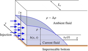
Figure 1. Diagram showing the set-up of axes and fluid orientation in flow through a narrow fracture (Hele-Shaw cell).
2 Model description for flow in a narrow fracture
The HB model for a shear-thinning/thickening fluid with yield stress is
 $$\begin{eqnarray}\left.\begin{array}{@{}c@{}}\unicode[STIX]{x1D70F}=(\unicode[STIX]{x1D707}_{0}\dot{\unicode[STIX]{x1D6FE}}^{n-1}+\unicode[STIX]{x1D70F}_{p}\dot{\unicode[STIX]{x1D6FE}}^{-1})\dot{\unicode[STIX]{x1D6FE}},\quad \unicode[STIX]{x1D70F}\geqslant \unicode[STIX]{x1D70F}_{p},\\ \dot{\unicode[STIX]{x1D6FE}}=0,\quad \unicode[STIX]{x1D70F}<\unicode[STIX]{x1D70F}_{p},\end{array}\right\}\end{eqnarray}$$
given in terms of the stress $\unicode[STIX]{x1D70F}$
and the strain rate
$\unicode[STIX]{x1D70F}$
and the strain rate $\dot{\unicode[STIX]{x1D6FE}}$
. A slightly more complicated description using tensor invariants is required for three-dimensional flows; this formulation is not reported here as we consider a one-dimensional problem below. The parameter
$\dot{\unicode[STIX]{x1D6FE}}$
. A slightly more complicated description using tensor invariants is required for three-dimensional flows; this formulation is not reported here as we consider a one-dimensional problem below. The parameter $\unicode[STIX]{x1D707}_{0}$
, the consistency index, represents a viscosity-like parameter, while
$\unicode[STIX]{x1D707}_{0}$
, the consistency index, represents a viscosity-like parameter, while $\unicode[STIX]{x1D70F}_{p}$
is the yield stress of the fluid, and
$\unicode[STIX]{x1D70F}_{p}$
is the yield stress of the fluid, and $n$
, the fluid behaviour index, controls the extent of shear thinning (
$n$
, the fluid behaviour index, controls the extent of shear thinning ( $n<1$
) or shear thickening (
$n<1$
) or shear thickening ( $n>1$
);
$n>1$
); $n=1$
corresponds to the Bingham case. For flow through a narrow fracture (such as a Hele-Shaw cell) of width
$n=1$
corresponds to the Bingham case. For flow through a narrow fracture (such as a Hele-Shaw cell) of width $L_{y}$
, as depicted in figure 1, the primary balance is between cross-gap quantities. The relevant relationship is that the velocity
$L_{y}$
, as depicted in figure 1, the primary balance is between cross-gap quantities. The relevant relationship is that the velocity $u(x,y)$
in the
$u(x,y)$
in the $x$
-direction must satisfy
$x$
-direction must satisfy
 $$\begin{eqnarray}\left.\begin{array}{@{}c@{}}\unicode[STIX]{x1D70F}_{xy}=\left(\unicode[STIX]{x1D707}_{0}\left|{\displaystyle \frac{\unicode[STIX]{x2202}u}{\unicode[STIX]{x2202}y}}\right|^{n-1}+\unicode[STIX]{x1D70F}_{p}\left|{\displaystyle \frac{\unicode[STIX]{x2202}u}{\unicode[STIX]{x2202}y}}\right|^{-1}\right){\displaystyle \frac{\unicode[STIX]{x2202}u}{\unicode[STIX]{x2202}y}},\quad \unicode[STIX]{x1D70F}_{xy}\geqslant \unicode[STIX]{x1D70F}_{p},\\ {\displaystyle \frac{\unicode[STIX]{x2202}u}{\unicode[STIX]{x2202}y}}=0,\quad \unicode[STIX]{x1D70F}_{xy}<\unicode[STIX]{x1D70F}_{p},\end{array}\right\}\end{eqnarray}$$
where $\unicode[STIX]{x1D70F}_{xy}$
represents the cross-gap stress and
$\unicode[STIX]{x1D70F}_{xy}$
represents the cross-gap stress and $y$
is the cross-gap direction. Furthermore, the primary balance between the cross-gap stress and the along-fracture pressure gradient is given by
$y$
is the cross-gap direction. Furthermore, the primary balance between the cross-gap stress and the along-fracture pressure gradient is given by $y(\unicode[STIX]{x2202}p/\unicode[STIX]{x2202}x)=\unicode[STIX]{x1D70F}_{xy}$
. We define the height
$y(\unicode[STIX]{x2202}p/\unicode[STIX]{x2202}x)=\unicode[STIX]{x1D70F}_{xy}$
. We define the height $h(x,t)$
of fluid above a horizontal impermeable base. Then, under the relevant shallow water approximation, the pressure is to leading order hydrostatic, and the pressure gradient becomes
$h(x,t)$
of fluid above a horizontal impermeable base. Then, under the relevant shallow water approximation, the pressure is to leading order hydrostatic, and the pressure gradient becomes $\unicode[STIX]{x2202}p/\unicode[STIX]{x2202}x=\unicode[STIX]{x0394}\unicode[STIX]{x1D70C}\,g\,(\unicode[STIX]{x2202}h/\unicode[STIX]{x2202}x)$
, where
$\unicode[STIX]{x2202}p/\unicode[STIX]{x2202}x=\unicode[STIX]{x0394}\unicode[STIX]{x1D70C}\,g\,(\unicode[STIX]{x2202}h/\unicode[STIX]{x2202}x)$
, where $\unicode[STIX]{x0394}\unicode[STIX]{x1D70C}$
is the density difference driving the flow, between fluid within and that outside the gravity current, and
$\unicode[STIX]{x0394}\unicode[STIX]{x1D70C}$
is the density difference driving the flow, between fluid within and that outside the gravity current, and $g$
is the acceleration due to gravity. We assume that the wetting characteristics at the walls of the fracture are unimportant (or alternatively that the flow takes place in a prewetted fracture). Combination of these equations, using the condition that
$g$
is the acceleration due to gravity. We assume that the wetting characteristics at the walls of the fracture are unimportant (or alternatively that the flow takes place in a prewetted fracture). Combination of these equations, using the condition that $\unicode[STIX]{x1D70F}_{xy}=\unicode[STIX]{x1D70F}_{p}$
as the fluid yields, leads to an expression for the location of the yield surface in the gap,
$\unicode[STIX]{x1D70F}_{xy}=\unicode[STIX]{x1D70F}_{p}$
as the fluid yields, leads to an expression for the location of the yield surface in the gap, $|y_{yield}|=\unicode[STIX]{x1D70F}_{p}/(\unicode[STIX]{x0394}\unicode[STIX]{x1D70C}\,g|\unicode[STIX]{x2202}h/\unicode[STIX]{x2202}x|)$
, where
$|y_{yield}|=\unicode[STIX]{x1D70F}_{p}/(\unicode[STIX]{x0394}\unicode[STIX]{x1D70C}\,g|\unicode[STIX]{x2202}h/\unicode[STIX]{x2202}x|)$
, where $-L_{y}/2\leqslant y_{yield}\leqslant L_{y}/2$
is required.
$-L_{y}/2\leqslant y_{yield}\leqslant L_{y}/2$
is required.
To continue, we need to solve for the cross-gap flow structure in yielded and unyielded regions of the flow. The continuity of mass of the fluid layer may be written as
 $$\begin{eqnarray}{\displaystyle \frac{\unicode[STIX]{x2202}h}{\unicode[STIX]{x2202}t}}=-{\displaystyle \frac{\unicode[STIX]{x2202}}{\unicode[STIX]{x2202}x}}(\bar{u}h),\end{eqnarray}$$
where $\bar{u}(x,t)$
is the gap-averaged velocity. Assuming a zero slip velocity, and upon introducing the expression for
$\bar{u}(x,t)$
is the gap-averaged velocity. Assuming a zero slip velocity, and upon introducing the expression for $\bar{u}(x,t)$
into (2.3), we can form an evolution equation for
$\bar{u}(x,t)$
into (2.3), we can form an evolution equation for $h(x,t)$
alone, namely
$h(x,t)$
alone, namely
 $$\begin{eqnarray}\displaystyle {\displaystyle \frac{\unicode[STIX]{x2202}h}{\unicode[STIX]{x2202}t}} & = & \displaystyle \left(\frac{L_{y}}{2}\right)^{(n+1)/n}\text{sgn}\left({\displaystyle \frac{\unicode[STIX]{x2202}h}{\unicode[STIX]{x2202}x}}\right)\left(\frac{n}{2n+1}\right)\left(\frac{\unicode[STIX]{x0394}\unicode[STIX]{x1D70C}\,g}{\unicode[STIX]{x1D707}_{0}}\right)^{1/n}\nonumber\\ \displaystyle & & \displaystyle \times \,{\displaystyle \frac{\unicode[STIX]{x2202}}{\unicode[STIX]{x2202}x}}\left[h\left|{\displaystyle \frac{\unicode[STIX]{x2202}h}{\unicode[STIX]{x2202}x}}\right|^{1/n}\left(1-\unicode[STIX]{x1D705}\left|{\displaystyle \frac{\unicode[STIX]{x2202}h}{\unicode[STIX]{x2202}x}}\right|^{-1}\right)^{(n+1)/n}\left(1+\left(\frac{n}{n+1}\right)\unicode[STIX]{x1D705}\left|{\displaystyle \frac{\unicode[STIX]{x2202}h}{\unicode[STIX]{x2202}x}}\right|^{-1}\right)\right],\end{eqnarray}$$
where $\unicode[STIX]{x1D705}=2\unicode[STIX]{x1D70F}_{p}/(\unicode[STIX]{x0394}\unicode[STIX]{x1D70C}\,gL_{y})$
is a non-dimensional number representing the ratio between yield stress and gravity related stress, or the ratio between the Bingham and Ramberg numbers. Additionally, setting
$\unicode[STIX]{x1D705}=2\unicode[STIX]{x1D70F}_{p}/(\unicode[STIX]{x0394}\unicode[STIX]{x1D70C}\,gL_{y})$
is a non-dimensional number representing the ratio between yield stress and gravity related stress, or the ratio between the Bingham and Ramberg numbers. Additionally, setting
 $$\begin{eqnarray}\unicode[STIX]{x1D6FA}=\left(\frac{L_{y}}{2}\right)^{(n+1)/n}\left(\frac{n}{2n+1}\right)\left(\frac{\unicode[STIX]{x0394}\unicode[STIX]{x1D70C}\,g}{\unicode[STIX]{x1D707}_{0}}\right)^{1/n},\end{eqnarray}$$
where $\unicode[STIX]{x1D6FA}$
is a velocity scale, allows us to write this equation slightly more succinctly as
$\unicode[STIX]{x1D6FA}$
is a velocity scale, allows us to write this equation slightly more succinctly as
 $$\begin{eqnarray}{\displaystyle \frac{\unicode[STIX]{x2202}h}{\unicode[STIX]{x2202}t}}=\text{sgn}\left({\displaystyle \frac{\unicode[STIX]{x2202}h}{\unicode[STIX]{x2202}x}}\right)\unicode[STIX]{x1D6FA}{\displaystyle \frac{\unicode[STIX]{x2202}}{\unicode[STIX]{x2202}x}}\left[h\left|{\displaystyle \frac{\unicode[STIX]{x2202}h}{\unicode[STIX]{x2202}x}}\right|^{1/n}\left(1-\unicode[STIX]{x1D705}\left|{\displaystyle \frac{\unicode[STIX]{x2202}h}{\unicode[STIX]{x2202}x}}\right|^{-1}\right)^{(n+1)/n}\left(1+\left(\frac{n}{n+1}\right)\unicode[STIX]{x1D705}\left|{\displaystyle \frac{\unicode[STIX]{x2202}h}{\unicode[STIX]{x2202}x}}\right|^{-1}\right)\right].\end{eqnarray}$$
To this equation we must add the further condition that when the flow is fully plugged (that is $y_{yield}=L_{y}/2$
), then the velocity throughout the gap is zero (
$y_{yield}=L_{y}/2$
), then the velocity throughout the gap is zero ( $\bar{u}=0$
), so therefore
$\bar{u}=0$
), so therefore $\unicode[STIX]{x2202}h/\unicode[STIX]{x2202}t=0$
for such regions. This is the limiting version of the equation above in the limit
$\unicode[STIX]{x2202}h/\unicode[STIX]{x2202}t=0$
for such regions. This is the limiting version of the equation above in the limit $\unicode[STIX]{x2202}h/\unicode[STIX]{x2202}x=\unicode[STIX]{x1D705}$
, which is in turn the condition for the flow to be fully plugged. Consequently, the equation for the height of the current is continuous through such a plugging transition.
$\unicode[STIX]{x2202}h/\unicode[STIX]{x2202}x=\unicode[STIX]{x1D705}$
, which is in turn the condition for the flow to be fully plugged. Consequently, the equation for the height of the current is continuous through such a plugging transition.
In the model, the slip contribution was neglected also because most experiments were conducted by roughening the Hele-Shaw cell with commercial transparent antislip tape, which is commonly adopted to make slippery surfaces safe. Independent rheometric measurements were conducted with plates roughened with sandpaper.
3 Self-similar solution
Various self-similar solutions exist to describe the spreading of gravity currents of constant or variable volume in cases similar to our problem where $\unicode[STIX]{x1D705}=0,n=1$
(e.g. King & Woods Reference King and Woods2003; Lyle et al.
Reference Lyle, Huppert, Hallworth, Bickle and Chadwick2005) and where
$\unicode[STIX]{x1D705}=0,n=1$
(e.g. King & Woods Reference King and Woods2003; Lyle et al.
Reference Lyle, Huppert, Hallworth, Bickle and Chadwick2005) and where $\unicode[STIX]{x1D705}=0$
(Pascal & Pascal Reference Pascal and Pascal1993; Longo et al.
Reference Longo, Di Federico, Chiapponi and Archetti2013b
; Longo, Di Federico & Chiapponi Reference Longo, Di Federico and Chiapponi2015b
; Ciriello et al.
Reference Ciriello, Longo, Chiapponi and Di Federico2016). For the current study where both yield stress and shear-thinning/thickening effects are present, a generalized form of such solutions is not available since the presence of yield stress breaks self-similarity. However, one form of self-similar solution does exist if we allow a variable injection rate of fluid (a more general type of solution with self-similarity of the second kind might be possible, although it is not attempted here). To this end, suppose that the volume of fluid in the gravity current varies as
$\unicode[STIX]{x1D705}=0$
(Pascal & Pascal Reference Pascal and Pascal1993; Longo et al.
Reference Longo, Di Federico, Chiapponi and Archetti2013b
; Longo, Di Federico & Chiapponi Reference Longo, Di Federico and Chiapponi2015b
; Ciriello et al.
Reference Ciriello, Longo, Chiapponi and Di Federico2016). For the current study where both yield stress and shear-thinning/thickening effects are present, a generalized form of such solutions is not available since the presence of yield stress breaks self-similarity. However, one form of self-similar solution does exist if we allow a variable injection rate of fluid (a more general type of solution with self-similarity of the second kind might be possible, although it is not attempted here). To this end, suppose that the volume of fluid in the gravity current varies as
 $$\begin{eqnarray}L_{y}\int _{0}^{\infty }h(x,t)\,\text{d}x=Qt^{\unicode[STIX]{x1D6FC}},\end{eqnarray}$$
where $\unicode[STIX]{x1D6FC},Q\geqslant 0$
. Then, the principal dimensions of the three parameters are
$\unicode[STIX]{x1D6FC},Q\geqslant 0$
. Then, the principal dimensions of the three parameters are $[\unicode[STIX]{x1D6FA}]=L/T,[Q/L_{y}]=L^{2}/T^{\unicode[STIX]{x1D6FC}},[\unicode[STIX]{x1D705}]=1.$
It is possible to rewrite our principal variables in dimensionless form as
$[\unicode[STIX]{x1D6FA}]=L/T,[Q/L_{y}]=L^{2}/T^{\unicode[STIX]{x1D6FC}},[\unicode[STIX]{x1D705}]=1.$
It is possible to rewrite our principal variables in dimensionless form as
 $$\begin{eqnarray}\widetilde{h}=h\left(\frac{Q}{L_{y}\unicode[STIX]{x1D6FA}^{\unicode[STIX]{x1D6FC}}}\right)^{1/(\unicode[STIX]{x1D6FC}-2)},\quad \widetilde{x}=x\left(\frac{Q}{L_{y}\unicode[STIX]{x1D6FA}^{\unicode[STIX]{x1D6FC}}}\right)^{1/(\unicode[STIX]{x1D6FC}-2)},\quad \widetilde{t}=t\left(\frac{Q}{L_{y}\unicode[STIX]{x1D6FA}^{2}}\right)^{1/(\unicode[STIX]{x1D6FC}-2)}.\end{eqnarray}$$
Introduction of these variables immediately reduces (2.6)–(3.1) to the dimensionless form
 $$\begin{eqnarray}{\displaystyle \frac{\unicode[STIX]{x2202}\widetilde{h}}{\unicode[STIX]{x2202}\widetilde{t}}}=-{\displaystyle \frac{\unicode[STIX]{x2202}}{\unicode[STIX]{x2202}\widetilde{x}}}\left[\widetilde{h}\left|{\displaystyle \frac{\unicode[STIX]{x2202}\widetilde{h}}{\unicode[STIX]{x2202}\widetilde{x}}}\right|^{1/n}\left(1-\unicode[STIX]{x1D705}\left|{\displaystyle \frac{\unicode[STIX]{x2202}\widetilde{h}}{\unicode[STIX]{x2202}\widetilde{x}}}\right|^{-1}\right)^{(n+1)/n}\left(1+\left(\frac{n}{n+1}\right)\unicode[STIX]{x1D705}\left|{\displaystyle \frac{\unicode[STIX]{x2202}\widetilde{h}}{\unicode[STIX]{x2202}\widetilde{x}}}\right|^{-1}\right)\right],\end{eqnarray}$$
 $$\begin{eqnarray}\int _{0}^{\infty }\widetilde{h}\,\text{d}\widetilde{x}=\widetilde{t}^{\,\unicode[STIX]{x1D6FC}},\end{eqnarray}$$
where we have assumed that $\unicode[STIX]{x2202}\widetilde{h}/\unicode[STIX]{x2202}\widetilde{x}<0$
. Hereafter, the tilde is dropped. We can seek self-similar solutions of these equations by looking for solutions in the form
$\unicode[STIX]{x2202}\widetilde{h}/\unicode[STIX]{x2202}\widetilde{x}<0$
. Hereafter, the tilde is dropped. We can seek self-similar solutions of these equations by looking for solutions in the form $h=t^{\unicode[STIX]{x1D6FD}}f(\unicode[STIX]{x1D702})$
, where
$h=t^{\unicode[STIX]{x1D6FD}}f(\unicode[STIX]{x1D702})$
, where $\unicode[STIX]{x1D702}=x/t^{\unicode[STIX]{x1D6FE}}$
. Substitution into (3.3)–(3.4) yields
$\unicode[STIX]{x1D702}=x/t^{\unicode[STIX]{x1D6FE}}$
. Substitution into (3.3)–(3.4) yields
 $$\begin{eqnarray}\displaystyle & \hspace{-6.0pt}\displaystyle \unicode[STIX]{x1D6FD}t^{\unicode[STIX]{x1D6FD}-1}f-t^{\unicode[STIX]{x1D6FD}-1}\unicode[STIX]{x1D6FE}\unicode[STIX]{x1D702}f^{\prime }=-\!\left[t^{\unicode[STIX]{x1D6FD}+(\unicode[STIX]{x1D6FD}-\unicode[STIX]{x1D6FE})/n}f|\,f^{\prime }|^{1/n}\!\left(\!1-\frac{\unicode[STIX]{x1D705}t^{\unicode[STIX]{x1D6FE}-\unicode[STIX]{x1D6FD}}}{|f^{\prime }|}\right)^{(n+1)/n}\!\!\left(\!1+\!\left(\frac{n}{n+1}\right)\!\frac{\unicode[STIX]{x1D705}t^{\unicode[STIX]{x1D6FE}-\unicode[STIX]{x1D6FD}}}{|f^{\prime }|}\right)\right]^{\prime }\!\!t^{-\unicode[STIX]{x1D6FE}}, & \displaystyle \nonumber\\ \displaystyle & & \displaystyle\end{eqnarray}$$
 $$\begin{eqnarray}\displaystyle & \displaystyle \int _{0}^{\unicode[STIX]{x1D702}_{e}}t^{\unicode[STIX]{x1D6FD}+\unicode[STIX]{x1D6FE}}f(\unicode[STIX]{x1D702})\,\text{d}\unicode[STIX]{x1D702}=t^{\unicode[STIX]{x1D6FC}}, & \displaystyle\end{eqnarray}$$
where primes denote differentiation with respect to $\unicode[STIX]{x1D702}$
. Comparison of powers of
$\unicode[STIX]{x1D702}$
. Comparison of powers of $t$
gives immediately
$t$
gives immediately $\unicode[STIX]{x1D6FD}+\unicode[STIX]{x1D6FE}=\unicode[STIX]{x1D6FC},\unicode[STIX]{x1D6FE}-\unicode[STIX]{x1D6FD}=0,\unicode[STIX]{x1D6FD}-1=(\unicode[STIX]{x1D6FD}-\unicode[STIX]{x1D6FE})(1+1/n)$
. This has one consistent solution, namely
$\unicode[STIX]{x1D6FD}+\unicode[STIX]{x1D6FE}=\unicode[STIX]{x1D6FC},\unicode[STIX]{x1D6FE}-\unicode[STIX]{x1D6FD}=0,\unicode[STIX]{x1D6FD}-1=(\unicode[STIX]{x1D6FD}-\unicode[STIX]{x1D6FE})(1+1/n)$
. This has one consistent solution, namely $\unicode[STIX]{x1D6FC}=2$
and
$\unicode[STIX]{x1D6FC}=2$
and $\unicode[STIX]{x1D6FD}=\unicode[STIX]{x1D6FE}=1$
. A fluid injection rate scaling as
$\unicode[STIX]{x1D6FD}=\unicode[STIX]{x1D6FE}=1$
. A fluid injection rate scaling as $t$
allows a self-similar solution, for which both the height and the length of the current increase with time, similarly scaling as
$t$
allows a self-similar solution, for which both the height and the length of the current increase with time, similarly scaling as $t$
. However, for
$t$
. However, for $\unicode[STIX]{x1D6FC}=2$
, the scales in (3.2) break down and an additional velocity scale embedded in the integral constraint of mass conservation given by (3.1) arises beyond
$\unicode[STIX]{x1D6FC}=2$
, the scales in (3.2) break down and an additional velocity scale embedded in the integral constraint of mass conservation given by (3.1) arises beyond $\unicode[STIX]{x1D6FA}$
, given by
$\unicode[STIX]{x1D6FA}$
, given by $(Q/L_{y})^{1/2}$
. A similar case is treated in Di Federico, Archetti & Longo (Reference Di Federico, Archetti and Longo2012a
,Reference Di Federico, Archetti and Longo
b
). We define an arbitrary time scale
$(Q/L_{y})^{1/2}$
. A similar case is treated in Di Federico, Archetti & Longo (Reference Di Federico, Archetti and Longo2012a
,Reference Di Federico, Archetti and Longo
b
). We define an arbitrary time scale $t^{\ast }$
, the velocity scale
$t^{\ast }$
, the velocity scale $u^{\ast }=(Q/L_{y})^{1/2}$
and the ratio between the two velocity scales
$u^{\ast }=(Q/L_{y})^{1/2}$
and the ratio between the two velocity scales $\unicode[STIX]{x1D6FF}=(L_{y}\unicode[STIX]{x1D6FA}^{2}/Q)^{1/2}$
, with
$\unicode[STIX]{x1D6FF}=(L_{y}\unicode[STIX]{x1D6FA}^{2}/Q)^{1/2}$
, with $x^{\ast }=u^{\ast }t^{\ast }$
. Equations (3.3)–(3.4) become
$x^{\ast }=u^{\ast }t^{\ast }$
. Equations (3.3)–(3.4) become
 $$\begin{eqnarray}\displaystyle & \displaystyle {\displaystyle \frac{\unicode[STIX]{x2202}h}{\unicode[STIX]{x2202}t}}=-\unicode[STIX]{x1D6FF}{\displaystyle \frac{\unicode[STIX]{x2202}}{\unicode[STIX]{x2202}x}}\left[h\left|{\displaystyle \frac{\unicode[STIX]{x2202}h}{\unicode[STIX]{x2202}x}}\right|^{1/n}\left(1-\unicode[STIX]{x1D705}\left|{\displaystyle \frac{\unicode[STIX]{x2202}h}{\unicode[STIX]{x2202}x}}\right|^{-1}\right)^{(n+1)/n}\left(1+\left(\frac{n}{n+1}\right)\unicode[STIX]{x1D705}\left|{\displaystyle \frac{\unicode[STIX]{x2202}h}{\unicode[STIX]{x2202}x}}\right|^{-1}\right)\right], & \displaystyle\end{eqnarray}$$
 $$\begin{eqnarray}\displaystyle & \displaystyle \int _{0}^{\infty }h(x,t)\,\text{d}x=t^{2}. & \displaystyle\end{eqnarray}$$
We seek a self-similar solution of the form $h=tf(\unicode[STIX]{x1D702}),\text{where}\quad \unicode[STIX]{x1D702}=x/t$
; substitution into (3.7)–(3.8) yields
$h=tf(\unicode[STIX]{x1D702}),\text{where}\quad \unicode[STIX]{x1D702}=x/t$
; substitution into (3.7)–(3.8) yields
 $$\begin{eqnarray}\displaystyle & \displaystyle f-\unicode[STIX]{x1D702}f^{\prime }=-\unicode[STIX]{x1D6FF}\left[f|\,f^{\prime }|^{1/n}\left(1-\frac{\unicode[STIX]{x1D705}}{|f^{\prime }|}\right)^{(n+1)/n}\left(1+\left(\frac{n}{n+1}\right)\frac{\unicode[STIX]{x1D705}}{|f^{\prime }|}\right)\right]^{\prime }, & \displaystyle\end{eqnarray}$$
 $$\begin{eqnarray}\displaystyle & \displaystyle \int _{0}^{\unicode[STIX]{x1D702}_{e}}f(\unicode[STIX]{x1D702})\,\text{d}\unicode[STIX]{x1D702}=1. & \displaystyle\end{eqnarray}$$
This system admits a simple solution, namely a linear profile for $f(\unicode[STIX]{x1D702})$
(Di Federico et al.
Reference Di Federico, Archetti and Longo2012a
). Supposing a solution in the form
$f(\unicode[STIX]{x1D702})$
(Di Federico et al.
Reference Di Federico, Archetti and Longo2012a
). Supposing a solution in the form $f(\unicode[STIX]{x1D702})=A(\unicode[STIX]{x1D702}_{e}-\unicode[STIX]{x1D702})$
, for some constants
$f(\unicode[STIX]{x1D702})=A(\unicode[STIX]{x1D702}_{e}-\unicode[STIX]{x1D702})$
, for some constants $A>0$
and
$A>0$
and $\unicode[STIX]{x1D702}_{e}>0$
, we substitute into (3.9)–(3.10) to obtain
$\unicode[STIX]{x1D702}_{e}>0$
, we substitute into (3.9)–(3.10) to obtain
 $$\begin{eqnarray}A\unicode[STIX]{x1D702}_{e}=\unicode[STIX]{x1D6FF}A^{(n+1)/n}\left(1-\frac{\unicode[STIX]{x1D705}}{A}\right)^{(n+1)/n}\left[1+\left(\frac{n}{n+1}\right)\frac{\unicode[STIX]{x1D705}}{A}\right],\quad \unicode[STIX]{x1D702}_{e}=\sqrt{\frac{2}{A}}.\end{eqnarray}$$
Elimination of $\unicode[STIX]{x1D702}_{e}$
gives one nonlinear equation to solve for
$\unicode[STIX]{x1D702}_{e}$
gives one nonlinear equation to solve for $A$
.
$A$
.
Solutions for several values of the parameter $n$
are shown in figure 2, with all other parameters kept constant. The self-similar solution retains similarity by constraining the yield surface to be at a constant location along its length as the current spreads. Furthermore, the thickness of the plugged region simply grows as the fluid becomes more shear thinning.
$n$
are shown in figure 2, with all other parameters kept constant. The self-similar solution retains similarity by constraining the yield surface to be at a constant location along its length as the current spreads. Furthermore, the thickness of the plugged region simply grows as the fluid becomes more shear thinning.
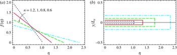
Figure 2. (a) Shape of the similarity solution in a Hele-Shaw cell ( $\unicode[STIX]{x1D6FC}=2$
) for different values of
$\unicode[STIX]{x1D6FC}=2$
) for different values of $n$
; (b) plug regions.
$n$
; (b) plug regions.
3.1 Asymptotic analysis for $\unicode[STIX]{x1D6FC}\neq 2$

For $\unicode[STIX]{x1D6FC}\neq 2$
, no self-similar solution is predicted, but it is possible to find an approximate result starting from the self-similar solution for power-law fluids (
$\unicode[STIX]{x1D6FC}\neq 2$
, no self-similar solution is predicted, but it is possible to find an approximate result starting from the self-similar solution for power-law fluids ( $\unicode[STIX]{x1D705}\rightarrow 0$
). We briefly recall that for
$\unicode[STIX]{x1D705}\rightarrow 0$
). We briefly recall that for $\unicode[STIX]{x1D705}\rightarrow 0$
equation (3.3) becomes
$\unicode[STIX]{x1D705}\rightarrow 0$
equation (3.3) becomes
 $$\begin{eqnarray}{\displaystyle \frac{\unicode[STIX]{x2202}h}{\unicode[STIX]{x2202}x}}=-{\displaystyle \frac{\unicode[STIX]{x2202}}{\unicode[STIX]{x2202}x}}\left(h\left|{\displaystyle \frac{\unicode[STIX]{x2202}h}{\unicode[STIX]{x2202}x}}\right|^{1/n}\right),\end{eqnarray}$$
while the integral mass balance given by (3.4) is unmodified. Equations (3.4)–(3.12) admit the similarity solution
 $$\begin{eqnarray}h=\unicode[STIX]{x1D702}_{N}^{n+2}t^{\,F_{2}}f(\unicode[STIX]{x1D701}),\quad \unicode[STIX]{x1D702}=xt^{\,-F_{1}},\quad \unicode[STIX]{x1D702}_{N}=\left(\int _{0}^{1}f\,\text{d}\unicode[STIX]{x1D701}\right)^{-1/(n+2)},\quad \unicode[STIX]{x1D701}=\unicode[STIX]{x1D702}/\unicode[STIX]{x1D702}_{N},\end{eqnarray}$$
where
 $$\begin{eqnarray}F_{1}={\displaystyle \frac{\unicode[STIX]{x1D6FC}+n}{2+n}},\quad F_{2}=\unicode[STIX]{x1D6FC}-F_{1},\end{eqnarray}$$
and where the shape function $f$
satisfies the following nonlinear ordinary differential equation:
$f$
satisfies the following nonlinear ordinary differential equation:
 $$\begin{eqnarray}(f|f^{\prime }|^{1/n})^{\prime }+F_{2}\,f-F_{1}\unicode[STIX]{x1D701}f^{\prime }=0.\end{eqnarray}$$
The numerical integration of (3.15) for $\unicode[STIX]{x1D6FC}\neq 0$
and
$\unicode[STIX]{x1D6FC}\neq 0$
and $\unicode[STIX]{x1D6FC}\neq 2$
requires two boundary conditions at
$\unicode[STIX]{x1D6FC}\neq 2$
requires two boundary conditions at $\unicode[STIX]{x1D701}\rightarrow 1$
. By assuming
$\unicode[STIX]{x1D701}\rightarrow 1$
. By assuming $f\approx a_{0}(1-\unicode[STIX]{x1D701})^{b}$
, substituting in (3.15) and balancing the lower-order terms,
$f\approx a_{0}(1-\unicode[STIX]{x1D701})^{b}$
, substituting in (3.15) and balancing the lower-order terms, $b=1$
and
$b=1$
and $a_{0}=F_{2}^{n}$
are yielded. Hence, it follows that
$a_{0}=F_{2}^{n}$
are yielded. Hence, it follows that
 $$\begin{eqnarray}\left.f\right|_{\unicode[STIX]{x1D701}\rightarrow 1-\unicode[STIX]{x1D716}}=F_{2}^{n}\unicode[STIX]{x1D716},\quad \left.f^{\prime }\right|_{\unicode[STIX]{x1D701}\rightarrow 1-\unicode[STIX]{x1D716}}=-F_{2}^{n},\end{eqnarray}$$
with $\unicode[STIX]{x1D716}$
a small quantity. The two cases
$\unicode[STIX]{x1D716}$
a small quantity. The two cases $\unicode[STIX]{x1D6FC}=0,2$
admit an analytical solution with
$\unicode[STIX]{x1D6FC}=0,2$
admit an analytical solution with $f$
represented by a parabola and a straight line respectively.
$f$
represented by a parabola and a straight line respectively.
It is possible to extend the self-similar solution to $\unicode[STIX]{x1D705}>0$
with the following expansion in the term
$\unicode[STIX]{x1D705}>0$
with the following expansion in the term $\unicode[STIX]{x1D705}/|\unicode[STIX]{x2202}h/\unicode[STIX]{x2202}x|$
(see, e.g., Hogg, Ungarish & Huppert Reference Hogg, Ungarish and Huppert2000; Sachdev Reference Sachdev2000).
$\unicode[STIX]{x1D705}/|\unicode[STIX]{x2202}h/\unicode[STIX]{x2202}x|$
(see, e.g., Hogg, Ungarish & Huppert Reference Hogg, Ungarish and Huppert2000; Sachdev Reference Sachdev2000).
Upon assuming that $\unicode[STIX]{x1D705}/|\unicode[STIX]{x2202}h/\unicode[STIX]{x2202}x|$
is a small quantity, (3.3) becomes
$\unicode[STIX]{x1D705}/|\unicode[STIX]{x2202}h/\unicode[STIX]{x2202}x|$
is a small quantity, (3.3) becomes
 $$\begin{eqnarray}{\displaystyle \frac{\unicode[STIX]{x2202}h}{\unicode[STIX]{x2202}t}}=-{\displaystyle \frac{\unicode[STIX]{x2202}}{\unicode[STIX]{x2202}x}}\left[h\left|{\displaystyle \frac{\unicode[STIX]{x2202}h}{\unicode[STIX]{x2202}x}}\right|^{1/n}\left(1-{\displaystyle \frac{2n+1}{n(n+1)}}\unicode[STIX]{x1D705}\left|{\displaystyle \frac{\unicode[STIX]{x2202}h}{\unicode[STIX]{x2202}x}}\right|^{-1}+{\displaystyle \frac{n+1-2n^{2}}{2n^{2}}}\unicode[STIX]{x1D705}^{2}\left|{\displaystyle \frac{\unicode[STIX]{x2202}h}{\unicode[STIX]{x2202}x}}\right|^{-2}+O(\unicode[STIX]{x1D705}^{3})\right)\right].\end{eqnarray}$$
We propose the following expansion in the regime $\unicode[STIX]{x1D70E}\equiv \unicode[STIX]{x1D705}t^{n(2-\unicode[STIX]{x1D6FC})/(n+2)}\ll 1$
:
$\unicode[STIX]{x1D70E}\equiv \unicode[STIX]{x1D705}t^{n(2-\unicode[STIX]{x1D6FC})/(n+2)}\ll 1$
:
 $$\begin{eqnarray}\displaystyle & \displaystyle h=\unicode[STIX]{x1D702}_{N}^{n+1}t^{F_{2}}[f_{0}(\unicode[STIX]{x1D701})+\unicode[STIX]{x1D70E}f_{1}(\unicode[STIX]{x1D701})+\unicode[STIX]{x1D70E}^{2}f_{2}(\unicode[STIX]{x1D701})+\cdots \,], & \displaystyle\end{eqnarray}$$
 $$\begin{eqnarray}\displaystyle & \displaystyle x=\unicode[STIX]{x1D702}t^{F_{1}}(1+\unicode[STIX]{x1D70E}X_{1}+\unicode[STIX]{x1D70E}^{2}X_{2}+\cdots \,), & \displaystyle\end{eqnarray}$$
where $f_{0}(\unicode[STIX]{x1D701})$
and
$f_{0}(\unicode[STIX]{x1D701})$
and $\unicode[STIX]{x1D702}_{N}$
are given by the similarity solution for power-law fluids (3.13), and
$\unicode[STIX]{x1D702}_{N}$
are given by the similarity solution for power-law fluids (3.13), and $X_{1},X_{2},\ldots$
are constants to be evaluated.
$X_{1},X_{2},\ldots$
are constants to be evaluated.
The variable $\unicode[STIX]{x1D70E}$
is selected in order to guarantee that at the zero order
$\unicode[STIX]{x1D70E}$
is selected in order to guarantee that at the zero order $O(\unicode[STIX]{x1D70E}^{0})$
the yield stress contribution is null and the solution is represented by (3.13). At the first order
$O(\unicode[STIX]{x1D70E}^{0})$
the yield stress contribution is null and the solution is represented by (3.13). At the first order $O(\unicode[STIX]{x1D70E})$
there is a balance between the terms due to the yield stress and all other terms. The condition
$O(\unicode[STIX]{x1D70E})$
there is a balance between the terms due to the yield stress and all other terms. The condition $\unicode[STIX]{x1D70E}\ll 1$
requires that
$\unicode[STIX]{x1D70E}\ll 1$
requires that $t\ll t_{c}\equiv \unicode[STIX]{x1D705}^{(n+2)/[n(\unicode[STIX]{x1D6FC}-2)]}$
if
$t\ll t_{c}\equiv \unicode[STIX]{x1D705}^{(n+2)/[n(\unicode[STIX]{x1D6FC}-2)]}$
if $\unicode[STIX]{x1D6FC}<2$
and
$\unicode[STIX]{x1D6FC}<2$
and $t\gg t_{c}$
if
$t\gg t_{c}$
if $\unicode[STIX]{x1D6FC}>2$
;
$\unicode[STIX]{x1D6FC}>2$
; $t_{c}$
is defined as a ‘critical time’. Figure 3 shows the critical time
$t_{c}$
is defined as a ‘critical time’. Figure 3 shows the critical time $t_{c}(\unicode[STIX]{x1D705},n,\unicode[STIX]{x1D6FC})$
for
$t_{c}(\unicode[STIX]{x1D705},n,\unicode[STIX]{x1D6FC})$
for $\unicode[STIX]{x1D705}=0.01$
and for different
$\unicode[STIX]{x1D705}=0.01$
and for different $n$
and
$n$
and $\unicode[STIX]{x1D6FC}$
. The critical time becomes infinite for
$\unicode[STIX]{x1D6FC}$
. The critical time becomes infinite for $\unicode[STIX]{x1D6FC}=2$
; notably, this coincides with the case that permits a self-similar solution without the necessity of an expansion. It is seen that
$\unicode[STIX]{x1D6FC}=2$
; notably, this coincides with the case that permits a self-similar solution without the necessity of an expansion. It is seen that $\unicode[STIX]{x2202}t_{c}/\unicode[STIX]{x2202}\unicode[STIX]{x1D6FC}>0$
for any
$\unicode[STIX]{x2202}t_{c}/\unicode[STIX]{x2202}\unicode[STIX]{x1D6FC}>0$
for any $n$
. In addition,
$n$
. In addition, $\unicode[STIX]{x2202}t_{c}/\unicode[STIX]{x2202}n>0$
if
$\unicode[STIX]{x2202}t_{c}/\unicode[STIX]{x2202}n>0$
if $\unicode[STIX]{x1D6FC}>2$
and
$\unicode[STIX]{x1D6FC}>2$
and $\unicode[STIX]{x2202}t_{c}/\unicode[STIX]{x2202}n<0$
if
$\unicode[STIX]{x2202}t_{c}/\unicode[STIX]{x2202}n<0$
if $\unicode[STIX]{x1D6FC}<2$
; hence, the domain of validity of the expansion is extended as the fluid becomes more shear thinning.
$\unicode[STIX]{x1D6FC}<2$
; hence, the domain of validity of the expansion is extended as the fluid becomes more shear thinning.
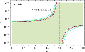
Figure 3. Dimensionless critical time for $\unicode[STIX]{x1D705}=0.01$
as a function of the fluid behaviour index
$\unicode[STIX]{x1D705}=0.01$
as a function of the fluid behaviour index $n$
and of
$n$
and of $\unicode[STIX]{x1D6FC}$
. The vertical dashed line at
$\unicode[STIX]{x1D6FC}$
. The vertical dashed line at $\unicode[STIX]{x1D6FC}=2$
is the asymptote; the hatched area indicates the domain where the condition
$\unicode[STIX]{x1D6FC}=2$
is the asymptote; the hatched area indicates the domain where the condition $\unicode[STIX]{x1D70E}<1$
is satisfied for a fluid with
$\unicode[STIX]{x1D70E}<1$
is satisfied for a fluid with $n=1.2$
.
$n=1.2$
.
The previous analysis implies that for a gravity current of a power-law fluid, all terms in the evolution equations evolve at a common rate (or, equivalently, a unique velocity scale exists). In contrast, for an HB fluid, the term arising due to the yield stress evolves at a different rate from other terms (i.e. it introduces a second velocity scale, for a given common length scale). In order to obtain an expansion to solve this equation, it should be noted that the correction is achieved at first order by computing a second function that evolves with a rate equal to the new one imposed by the yield stress term. The nonlinearity of the problem requires an increasing number of such terms in the series to improve the accuracy in the balance when extended to higher orders.
However, since $\unicode[STIX]{x1D705}$
appears always in powers of
$\unicode[STIX]{x1D705}$
appears always in powers of $\unicode[STIX]{x1D705}|\unicode[STIX]{x2202}h/\unicode[STIX]{x2202}x|^{-1}$
, we expect a reduction in the accuracy of the asymptotic solution for increasing time, if
$\unicode[STIX]{x1D705}|\unicode[STIX]{x2202}h/\unicode[STIX]{x2202}x|^{-1}$
, we expect a reduction in the accuracy of the asymptotic solution for increasing time, if $\overline{|\unicode[STIX]{x2202}h/\unicode[STIX]{x2202}x|}\sim t^{(\unicode[STIX]{x1D6FC}-2)n/(n+2)}$
decreases in time, which happens for
$\overline{|\unicode[STIX]{x2202}h/\unicode[STIX]{x2202}x|}\sim t^{(\unicode[STIX]{x1D6FC}-2)n/(n+2)}$
decreases in time, which happens for $\unicode[STIX]{x1D6FC}<2$
. Conversely, for
$\unicode[STIX]{x1D6FC}<2$
. Conversely, for $\unicode[STIX]{x1D6FC}>2$
, the asymptotic expansion becomes more accurate, but the current evolves to an increasing steepness which renders the thin-current assumption asymptotically invalid. The expansion will be uniform in
$\unicode[STIX]{x1D6FC}>2$
, the asymptotic expansion becomes more accurate, but the current evolves to an increasing steepness which renders the thin-current assumption asymptotically invalid. The expansion will be uniform in $x$
as long as
$x$
as long as $|\unicode[STIX]{x2202}h/\unicode[STIX]{x2202}x|$
does not approach zero anywhere. In particular, the expansion will be non-uniform if
$|\unicode[STIX]{x2202}h/\unicode[STIX]{x2202}x|$
does not approach zero anywhere. In particular, the expansion will be non-uniform if $\unicode[STIX]{x1D6FC}=0$
, since in this case the current becomes flat at
$\unicode[STIX]{x1D6FC}=0$
, since in this case the current becomes flat at $x=0$
.
$x=0$
.
By inserting (3.18)–(3.19) in (3.17) and balancing the terms of equal power in $\unicode[STIX]{x1D70E}$
, at
$\unicode[STIX]{x1D70E}$
, at $O(\unicode[STIX]{x1D70E}^{0})$
we recover the fundamental balance, with
$O(\unicode[STIX]{x1D70E}^{0})$
we recover the fundamental balance, with $f_{0}\equiv f$
, and
$f_{0}\equiv f$
, and $f$
represented by (3.13).
$f$
represented by (3.13).
At $O(\unicode[STIX]{x1D70E})$
, equation (3.17) becomes
$O(\unicode[STIX]{x1D70E})$
, equation (3.17) becomes
 $$\begin{eqnarray}\left(f_{1}|f_{0}^{\prime }|^{1/n}-{\displaystyle \frac{1}{n}}f_{0}|f_{0}^{\prime }|^{1/n-1}f_{1}^{\prime }\right)^{\prime }+F_{2}f_{1}-F_{1}\unicode[STIX]{x1D701}f_{1}^{\prime }={\displaystyle \frac{1}{\unicode[STIX]{x1D702}_{N}^{n}}}{\displaystyle \frac{2n+1}{n(n+1)}}(f_{0}|f_{0}^{\prime }|^{1/n-1})^{\prime },\end{eqnarray}$$
which is an inhomogeneous linear ordinary differential equation for the unknown function $f_{1}$
, with a forcing term modulated by the fundamental solution
$f_{1}$
, with a forcing term modulated by the fundamental solution $f_{0}$
. The numerical integration of equation (3.20) requires two boundary conditions for
$f_{0}$
. The numerical integration of equation (3.20) requires two boundary conditions for $\unicode[STIX]{x1D701}\rightarrow 1$
, obtained again by expanding in series near the front of the current. Assuming that
$\unicode[STIX]{x1D701}\rightarrow 1$
, obtained again by expanding in series near the front of the current. Assuming that $f_{1}\approx a_{1}(1-\unicode[STIX]{x1D701})^{b}$
(with
$f_{1}\approx a_{1}(1-\unicode[STIX]{x1D701})^{b}$
(with $f_{0}\approx F_{2}^{n}(1-\unicode[STIX]{x1D701})$
, see (3.16)), substituting in (3.20) and equating the lower-order terms (corresponding to
$f_{0}\approx F_{2}^{n}(1-\unicode[STIX]{x1D701})$
, see (3.16)), substituting in (3.20) and equating the lower-order terms (corresponding to $b=1$
) yields
$b=1$
) yields
 $$\begin{eqnarray}a_{1}={\displaystyle \frac{F_{2}}{(F_{2}-F_{1}n+F_{2}n)}}{\displaystyle \frac{2n+1}{\unicode[STIX]{x1D702}_{N}^{n}(n+1)}},\quad b=1.\end{eqnarray}$$
Hence, the function can be approximated by $f_{1}\approx a_{1}(1-\unicode[STIX]{x1D701})$
for
$f_{1}\approx a_{1}(1-\unicode[STIX]{x1D701})$
for $\unicode[STIX]{x1D701}\rightarrow 1$
, and the boundary conditions for equation (3.20) are
$\unicode[STIX]{x1D701}\rightarrow 1$
, and the boundary conditions for equation (3.20) are
 $$\begin{eqnarray}\left.f_{1}\right|_{\unicode[STIX]{x1D701}\rightarrow 1-\unicode[STIX]{x1D716}}=a_{1}\unicode[STIX]{x1D716},\quad f_{1}^{\prime }|_{\unicode[STIX]{x1D701}\rightarrow 1-\unicode[STIX]{x1D716}}=-a_{1},\end{eqnarray}$$
where $\unicode[STIX]{x1D716}$
is a small quantity.
$\unicode[STIX]{x1D716}$
is a small quantity.
Even though the two functions $f_{0}$
and
$f_{0}$
and $f_{1}$
are defined in the domain
$f_{1}$
are defined in the domain $0\leqslant \unicode[STIX]{x1D701}\leqslant 1$
, the nose of the current is
$0\leqslant \unicode[STIX]{x1D701}\leqslant 1$
, the nose of the current is $\unicode[STIX]{x1D701}_{N}=1+\unicode[STIX]{x1D70E}X_{1}+\cdots \,,$
which is expected to be smaller than unity since the additional resistance supplied by the yield stress reduces the propagation rate compared with the case
$\unicode[STIX]{x1D701}_{N}=1+\unicode[STIX]{x1D70E}X_{1}+\cdots \,,$
which is expected to be smaller than unity since the additional resistance supplied by the yield stress reduces the propagation rate compared with the case $\unicode[STIX]{x1D705}=0$
. The integral constraint given by (3.4) becomes
$\unicode[STIX]{x1D705}=0$
. The integral constraint given by (3.4) becomes
 $$\begin{eqnarray}\unicode[STIX]{x1D702}_{N}^{n+2}(1+\unicode[STIX]{x1D70E}X_{1}+\cdots \,)\int _{0}^{1+\unicode[STIX]{x1D70E}X_{1}+\cdots }[f_{0}(\unicode[STIX]{x1D701})+\unicode[STIX]{x1D70E}f_{1}(\unicode[STIX]{x1D701})]\,\text{d}\unicode[STIX]{x1D701}=1,\end{eqnarray}$$
which at $O(\unicode[STIX]{x1D70E})$
yields
$O(\unicode[STIX]{x1D70E})$
yields
 $$\begin{eqnarray}X_{1}=-{\displaystyle \frac{\displaystyle \int _{0}^{1}f_{1}(\unicode[STIX]{x1D701})\,\text{d}\unicode[STIX]{x1D701}}{\displaystyle \int _{0}^{1}f_{0}(\unicode[STIX]{x1D701})\,\text{d}\unicode[STIX]{x1D701}}}.\end{eqnarray}$$
Figure 4 shows the correction to the front position for waning inflow rate ( $\unicode[STIX]{x1D6FC}=0.5$
), constant inflow rate (
$\unicode[STIX]{x1D6FC}=0.5$
), constant inflow rate ( $\unicode[STIX]{x1D6FC}=1$
), waxing inflow rate (
$\unicode[STIX]{x1D6FC}=1$
), waxing inflow rate ( $\unicode[STIX]{x1D6FC}=1.5$
) and very waxing inflow rate (
$\unicode[STIX]{x1D6FC}=1.5$
) and very waxing inflow rate ( $\unicode[STIX]{x1D6FC}=2.5$
). The case
$\unicode[STIX]{x1D6FC}=2.5$
). The case $\unicode[STIX]{x1D6FC}=2$
is not shown since the correction is null. The smallest correction is for waxing inflow rates, with minimum effects for shear-thickening fluids, while for low values of
$\unicode[STIX]{x1D6FC}=2$
is not shown since the correction is null. The smallest correction is for waxing inflow rates, with minimum effects for shear-thickening fluids, while for low values of $\unicode[STIX]{x1D6FC}$
, the corrections are minor for shear-thinning fluids. The first-order correction term may be valid for a limited time, as shown in figure 4(a) for shear-thickening and Newtonian fluids with
$\unicode[STIX]{x1D6FC}$
, the corrections are minor for shear-thinning fluids. The first-order correction term may be valid for a limited time, as shown in figure 4(a) for shear-thickening and Newtonian fluids with $\unicode[STIX]{x1D705}=0.05$
; a divergence from the first-order approximation solution appears for
$\unicode[STIX]{x1D705}=0.05$
; a divergence from the first-order approximation solution appears for $t<10$
and
$t<10$
and $t<20$
respectively. Since the critical times are
$t<20$
respectively. Since the critical times are $t_{c}\approx 100$
and
$t_{c}\approx 100$
and $t_{c}\approx 400$
for the two cases, we conclude that the limiting factor is the number of terms in the expansion. An extension of the range of validity can be achieved by increasing the number of these terms (see, e.g., Hogg et al.
Reference Hogg, Ungarish and Huppert2000).
$t_{c}\approx 400$
for the two cases, we conclude that the limiting factor is the number of terms in the expansion. An extension of the range of validity can be achieved by increasing the number of these terms (see, e.g., Hogg et al.
Reference Hogg, Ungarish and Huppert2000).
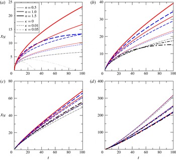
Figure 4. The effects of the first-order correction on the front position, for a Hele-Shaw cell: (a) $\unicode[STIX]{x1D6FC}=0.5$
, (b)
$\unicode[STIX]{x1D6FC}=0.5$
, (b) $\unicode[STIX]{x1D6FC}=1$
, (c)
$\unicode[STIX]{x1D6FC}=1$
, (c) $\unicode[STIX]{x1D6FC}=1.5$
, (d)
$\unicode[STIX]{x1D6FC}=1.5$
, (d) $\unicode[STIX]{x1D6FC}=2.5$
. The thick, mid and thin curves refer to
$\unicode[STIX]{x1D6FC}=2.5$
. The thick, mid and thin curves refer to $n=1.5$
,
$n=1.5$
, $n=1$
and
$n=1$
and $n=0.5$
respectively. The continuous, dashed and dot-dashed curves refer to
$n=0.5$
respectively. The continuous, dashed and dot-dashed curves refer to $\unicode[STIX]{x1D705}=0$
(power-law fluid),
$\unicode[STIX]{x1D705}=0$
(power-law fluid), $\unicode[STIX]{x1D705}=0.01$
and
$\unicode[STIX]{x1D705}=0.01$
and $\unicode[STIX]{x1D705}=0.05$
respectively. The time decreasing curves, in grey, are unphysical. Variables are non-dimensional.
$\unicode[STIX]{x1D705}=0.05$
respectively. The time decreasing curves, in grey, are unphysical. Variables are non-dimensional.
Figure 5 shows the profiles of the current at $t=5$
for constant volume (
$t=5$
for constant volume ( $\unicode[STIX]{x1D6FC}=0$
) and constant inflow rate (
$\unicode[STIX]{x1D6FC}=0$
) and constant inflow rate ( $\unicode[STIX]{x1D6FC}=1$
). The case
$\unicode[STIX]{x1D6FC}=1$
). The case $\unicode[STIX]{x1D6FC}=0,\unicode[STIX]{x1D705}=0$
has a closed-form solution (Ciriello et al.
Reference Ciriello, Longo, Chiapponi and Di Federico2016) and is a parabola for a Newtonian fluid (
$\unicode[STIX]{x1D6FC}=0,\unicode[STIX]{x1D705}=0$
has a closed-form solution (Ciriello et al.
Reference Ciriello, Longo, Chiapponi and Di Federico2016) and is a parabola for a Newtonian fluid ( $n=1$
). The presence of yield stress reduces the front position and increases the average steepness of the profile, without other significant variations as long as
$n=1$
). The presence of yield stress reduces the front position and increases the average steepness of the profile, without other significant variations as long as $\unicode[STIX]{x1D705}$
is a small quantity.
$\unicode[STIX]{x1D705}$
is a small quantity.
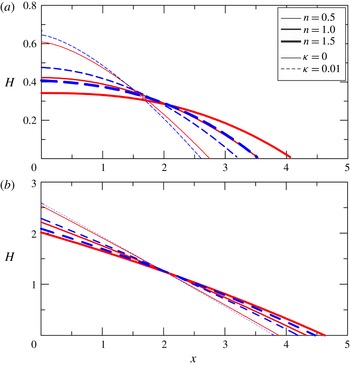
Figure 5. The effects of the first-order correction on the current profiles at time $t=5$
, for a Hele-Shaw cell: (a)
$t=5$
, for a Hele-Shaw cell: (a) $\unicode[STIX]{x1D6FC}=0$
, (b)
$\unicode[STIX]{x1D6FC}=0$
, (b) $\unicode[STIX]{x1D6FC}=1$
. The thick, mid and thin curves refer to
$\unicode[STIX]{x1D6FC}=1$
. The thick, mid and thin curves refer to $n=1.5$
,
$n=1.5$
, $n=1$
and
$n=1$
and $n=0.5$
respectively. The continuous and dashed curves refer to
$n=0.5$
respectively. The continuous and dashed curves refer to $\unicode[STIX]{x1D705}=0$
(power-law fluid) and
$\unicode[STIX]{x1D705}=0$
(power-law fluid) and $\unicode[STIX]{x1D705}=0.01$
respectively. Variables are non-dimensional.
$\unicode[STIX]{x1D705}=0.01$
respectively. Variables are non-dimensional.
4 Two-dimensional flow in a porous medium
The case of flow through a porous medium requires the formulation of the equivalent Darcy’s law for an HB fluid, which may be written as (Chevalier et al. Reference Chevalier, Chevalier, Clain, Dupla, Canou, Rodts and Coussot2013)
 $$\begin{eqnarray}d\unicode[STIX]{x1D735}p=\unicode[STIX]{x1D712}\unicode[STIX]{x1D70F}_{p}+\unicode[STIX]{x1D6FD}\unicode[STIX]{x1D707}_{0}\left({\displaystyle \frac{\bar{u}}{d}}\right)^{n},\end{eqnarray}$$
where $d$
is the diameter of grains,
$d$
is the diameter of grains, $\unicode[STIX]{x1D735}p$
is the pressure gradient,
$\unicode[STIX]{x1D735}p$
is the pressure gradient, $\unicode[STIX]{x1D70F}_{p}$
is the yield stress,
$\unicode[STIX]{x1D70F}_{p}$
is the yield stress, $\unicode[STIX]{x1D707}_{0}$
is the consistency index,
$\unicode[STIX]{x1D707}_{0}$
is the consistency index, $n$
is the flow behaviour index,
$n$
is the flow behaviour index, $\bar{u}$
is the Darcian velocity, and
$\bar{u}$
is the Darcian velocity, and $\unicode[STIX]{x1D712}$
and
$\unicode[STIX]{x1D712}$
and $\unicode[STIX]{x1D6FD}$
are coefficients. The coefficient
$\unicode[STIX]{x1D6FD}$
are coefficients. The coefficient $\unicode[STIX]{x1D712}$
is governed by the maximum width of the widest path of the flowing current while the coefficient
$\unicode[STIX]{x1D712}$
is governed by the maximum width of the widest path of the flowing current while the coefficient $\unicode[STIX]{x1D6FD}$
depends on pore size distribution and structure. Their values should, in general, be determined experimentally, and theoretically they are related to the distribution of the second invariant of the strain tensor (Chevalier et al.
Reference Chevalier, Rodts, Chateau, Chevalier and Coussot2014). Here, a pragmatic approach is adopted, and the values reported in Chevalier et al. (Reference Chevalier, Chevalier, Clain, Dupla, Canou, Rodts and Coussot2013),
$\unicode[STIX]{x1D6FD}$
depends on pore size distribution and structure. Their values should, in general, be determined experimentally, and theoretically they are related to the distribution of the second invariant of the strain tensor (Chevalier et al.
Reference Chevalier, Rodts, Chateau, Chevalier and Coussot2014). Here, a pragmatic approach is adopted, and the values reported in Chevalier et al. (Reference Chevalier, Chevalier, Clain, Dupla, Canou, Rodts and Coussot2013), $\unicode[STIX]{x1D712}=5.5$
and
$\unicode[STIX]{x1D712}=5.5$
and $\unicode[STIX]{x1D6FD}=85$
, are used; the diameter of the glass beads employed in our experiments falls in the range adopted in their experiments (from 0.26 to 2 mm). Equation (4.1) indicates that the flow is possible only if
$\unicode[STIX]{x1D6FD}=85$
, are used; the diameter of the glass beads employed in our experiments falls in the range adopted in their experiments (from 0.26 to 2 mm). Equation (4.1) indicates that the flow is possible only if $|\unicode[STIX]{x2202}p/\unicode[STIX]{x2202}x|>\unicode[STIX]{x1D712}\unicode[STIX]{x1D70F}_{p}/d$
; otherwise a plug is formed. Indeed, the experiments indicate that percolation takes place even at a very low pressure gradient, with a progressive increment of the flow rate for increasing pressure drop. Chevalier et al. (Reference Chevalier, Rodts, Chateau, Chevalier and Coussot2014) have shown that even at very low Darcian velocity values, the region of fluid at rest is negligible and the velocity density distribution is similar to that obtained for a Newtonian fluid.
$|\unicode[STIX]{x2202}p/\unicode[STIX]{x2202}x|>\unicode[STIX]{x1D712}\unicode[STIX]{x1D70F}_{p}/d$
; otherwise a plug is formed. Indeed, the experiments indicate that percolation takes place even at a very low pressure gradient, with a progressive increment of the flow rate for increasing pressure drop. Chevalier et al. (Reference Chevalier, Rodts, Chateau, Chevalier and Coussot2014) have shown that even at very low Darcian velocity values, the region of fluid at rest is negligible and the velocity density distribution is similar to that obtained for a Newtonian fluid.
Under the relevant shallow water approximation, the pressure gradient becomes $\unicode[STIX]{x2202}p/\unicode[STIX]{x2202}x=\unicode[STIX]{x0394}\unicode[STIX]{x1D70C}\,g\,(\unicode[STIX]{x2202}h/\unicode[STIX]{x2202}x)$
; inverting (4.1), and under the constraint
$\unicode[STIX]{x2202}p/\unicode[STIX]{x2202}x=\unicode[STIX]{x0394}\unicode[STIX]{x1D70C}\,g\,(\unicode[STIX]{x2202}h/\unicode[STIX]{x2202}x)$
; inverting (4.1), and under the constraint $|\unicode[STIX]{x2202}h/\unicode[STIX]{x2202}x|>\unicode[STIX]{x1D705}_{p}$
, the average velocity is equal to
$|\unicode[STIX]{x2202}h/\unicode[STIX]{x2202}x|>\unicode[STIX]{x1D705}_{p}$
, the average velocity is equal to
 $$\begin{eqnarray}\bar{u}=-\text{sgn}\left({\displaystyle \frac{\unicode[STIX]{x2202}h}{\unicode[STIX]{x2202}x}}\right)d^{(n+1)/n}\left({\displaystyle \frac{\unicode[STIX]{x0394}\unicode[STIX]{x1D70C}\,g}{85\unicode[STIX]{x1D707}_{0}}}\right)^{1/n}\left(1-\unicode[STIX]{x1D705}_{p}\left|{\displaystyle \frac{\unicode[STIX]{x2202}h}{\unicode[STIX]{x2202}x}}\right|^{-1}\right)^{1/n}\left|{\displaystyle \frac{\unicode[STIX]{x2202}h}{\unicode[STIX]{x2202}x}}\right|^{1/n},\end{eqnarray}$$
where $\unicode[STIX]{x1D705}_{p}=5.5\unicode[STIX]{x1D70F}_{p}/(d\unicode[STIX]{x0394}\unicode[STIX]{x1D70C}\,g)$
. Insertion of the average velocity in the local mass conservation yields for
$\unicode[STIX]{x1D705}_{p}=5.5\unicode[STIX]{x1D70F}_{p}/(d\unicode[STIX]{x0394}\unicode[STIX]{x1D70C}\,g)$
. Insertion of the average velocity in the local mass conservation yields for $\unicode[STIX]{x2202}h/\unicode[STIX]{x2202}x<0$
 $$\begin{eqnarray}{\displaystyle \frac{\unicode[STIX]{x2202}h}{\unicode[STIX]{x2202}t}}=-{\displaystyle \frac{d^{(n+1)/n}}{\unicode[STIX]{x1D719}}}\left(\frac{\unicode[STIX]{x0394}\unicode[STIX]{x1D70C}\,g}{85\unicode[STIX]{x1D707}_{0}}\right)^{1/n}{\displaystyle \frac{\unicode[STIX]{x2202}}{\unicode[STIX]{x2202}x}}\left[h\left|{\displaystyle \frac{\unicode[STIX]{x2202}h}{\unicode[STIX]{x2202}x}}\right|^{1/n}\left(1-\unicode[STIX]{x1D705}_{p}\left|{\displaystyle \frac{\unicode[STIX]{x2202}h}{\unicode[STIX]{x2202}x}}\right|^{-1}\right)^{1/n}\right],\end{eqnarray}$$
where $\unicode[STIX]{x1D719}$
is the porosity. Assuming again a current with time variable volume, the integral mass conservation reads
$\unicode[STIX]{x1D719}$
is the porosity. Assuming again a current with time variable volume, the integral mass conservation reads
 $$\begin{eqnarray}L_{y}\unicode[STIX]{x1D719}\int _{0}^{\infty }h(x,t)\,\text{d}x=Qt^{\unicode[STIX]{x1D6FC}}.\end{eqnarray}$$
Upon introducing the velocity and length scales
 $$\begin{eqnarray}\displaystyle & \displaystyle u^{\ast }={\displaystyle \frac{d^{(n+1)/n}}{\unicode[STIX]{x1D719}}}\left(\frac{\unicode[STIX]{x0394}\unicode[STIX]{x1D70C}\,g}{85\unicode[STIX]{x1D707}_{0}}\right)^{1/n}, & \displaystyle\end{eqnarray}$$
 $$\begin{eqnarray}\displaystyle & \displaystyle x^{\ast }={\displaystyle \frac{d^{(n+1)/n}}{\unicode[STIX]{x1D719}}}\left({\displaystyle \frac{Q\unicode[STIX]{x1D719}}{L_{y}d^{(2n+2)/n}}}\right)^{1/(2-\unicode[STIX]{x1D6FC})}\left({\displaystyle \frac{85\unicode[STIX]{x1D707}_{0}}{\unicode[STIX]{x0394}\unicode[STIX]{x1D70C}\,g}}\right)^{\unicode[STIX]{x1D6FC}/[n(2-\unicode[STIX]{x1D6FC})]}, & \displaystyle\end{eqnarray}$$
with the resulting time scale
 $$\begin{eqnarray}t^{\ast }={\displaystyle \frac{x^{\ast }}{u^{\ast }}}=\left({\displaystyle \frac{Q\unicode[STIX]{x1D719}}{L_{y}d^{(2n+2)/n}}}\right)^{1/(2-\unicode[STIX]{x1D6FC})}\left({\displaystyle \frac{85\unicode[STIX]{x1D707}_{0}}{\unicode[STIX]{x0394}\unicode[STIX]{x1D70C}\,g}}\right)^{2/[n(2-\unicode[STIX]{x1D6FC})]},\end{eqnarray}$$
equations (4.3)–(4.4) may be written in non-dimensional form as
 $$\begin{eqnarray}\displaystyle & \displaystyle {\displaystyle \frac{\unicode[STIX]{x2202}h}{\unicode[STIX]{x2202}t}}=-{\displaystyle \frac{\unicode[STIX]{x2202}}{\unicode[STIX]{x2202}x}}\left[h\left|{\displaystyle \frac{\unicode[STIX]{x2202}h}{\unicode[STIX]{x2202}x}}\right|^{1/n}\left(1-\unicode[STIX]{x1D705}_{p}\left|{\displaystyle \frac{\unicode[STIX]{x2202}h}{\unicode[STIX]{x2202}x}}\right|^{-1}\right)^{1/n}\right], & \displaystyle\end{eqnarray}$$
 $$\begin{eqnarray}\displaystyle & \displaystyle \int _{0}^{\infty }h(x,t)\,\text{d}x=t^{\unicode[STIX]{x1D6FC}}. & \displaystyle\end{eqnarray}$$
As for the flow in the fracture, equations (4.8)–(4.9) admit a self-similar solution only for $\unicode[STIX]{x1D6FC}=2$
, which breaks down the scales in (4.6)–(4.7). By defining an arbitrary time scale
$\unicode[STIX]{x1D6FC}=2$
, which breaks down the scales in (4.6)–(4.7). By defining an arbitrary time scale $t^{\ast }$
, the new velocity scale
$t^{\ast }$
, the new velocity scale $u^{\ast }=(Q/L_{y}\unicode[STIX]{x1D719})^{1/2}$
and the coefficient
$u^{\ast }=(Q/L_{y}\unicode[STIX]{x1D719})^{1/2}$
and the coefficient
 $$\begin{eqnarray}\unicode[STIX]{x1D6FF}_{p}=\left({\displaystyle \frac{L_{y}d^{(2n+2)/n}}{Q\unicode[STIX]{x1D719}}}\right)^{1/2}\left({\displaystyle \frac{\unicode[STIX]{x0394}\unicode[STIX]{x1D70C}\,g}{85\unicode[STIX]{x1D707}_{0}}}\right)^{1/n},\end{eqnarray}$$
which is the ratio between the velocity scale (4.5) and the new velocity scale, (4.3) may be written in non-dimensional form (the tilde is dropped) as
 $$\begin{eqnarray}{\displaystyle \frac{\unicode[STIX]{x2202}h}{\unicode[STIX]{x2202}t}}=-\unicode[STIX]{x1D6FF}_{p}{\displaystyle \frac{\unicode[STIX]{x2202}}{\unicode[STIX]{x2202}x}}\left[h\left|{\displaystyle \frac{\unicode[STIX]{x2202}h}{\unicode[STIX]{x2202}x}}\right|^{1/n}\left(1-\unicode[STIX]{x1D705}_{p}\left|{\displaystyle \frac{\unicode[STIX]{x2202}h}{\unicode[STIX]{x2202}x}}\right|^{-1}\right)^{1/n}\right],\end{eqnarray}$$
while (4.4) becomes
 $$\begin{eqnarray}\int _{0}^{\infty }h(x,t)\,\text{d}x=t^{2}.\end{eqnarray}$$
The self-similar solution is again $h=tf(\unicode[STIX]{x1D702}),\unicode[STIX]{x1D702}=x/t$
, and substitution into (4.11) gives
$h=tf(\unicode[STIX]{x1D702}),\unicode[STIX]{x1D702}=x/t$
, and substitution into (4.11) gives
 $$\begin{eqnarray}f-\unicode[STIX]{x1D702}f^{\prime }=-\unicode[STIX]{x1D6FF}_{p}\left[f|f^{\prime }|^{1/n}\left(1-{\displaystyle \frac{\unicode[STIX]{x1D705}_{p}}{|f^{\prime }|}}\right)^{1/n}\right]^{\prime }.\end{eqnarray}$$
The system of equations (4.11)–(4.12) admits a solution $f(\unicode[STIX]{x1D702})=A_{p}(\unicode[STIX]{x1D702}_{ep}-\unicode[STIX]{x1D702})$
, which upon substitution yields
$f(\unicode[STIX]{x1D702})=A_{p}(\unicode[STIX]{x1D702}_{ep}-\unicode[STIX]{x1D702})$
, which upon substitution yields
 $$\begin{eqnarray}{\displaystyle \frac{2}{A_{p}}}=\unicode[STIX]{x1D6FF}_{p}^{2}(A_{p}-\unicode[STIX]{x1D705}_{p})^{2/n},\quad A_{p}\unicode[STIX]{x1D702}_{ep}^{2}=2.\end{eqnarray}$$
For given values of $\unicode[STIX]{x1D705}_{p}$
and
$\unicode[STIX]{x1D705}_{p}$
and $\unicode[STIX]{x1D6FF}_{p}$
, it is possible to solve the first equation numerically in the unknown
$\unicode[STIX]{x1D6FF}_{p}$
, it is possible to solve the first equation numerically in the unknown $A_{p}$
and then to compute
$A_{p}$
and then to compute $\unicode[STIX]{x1D702}_{ep}$
. The condition for flow requires that
$\unicode[STIX]{x1D702}_{ep}$
. The condition for flow requires that $A_{P}>\unicode[STIX]{x1D705}_{p}$
. The general case
$A_{P}>\unicode[STIX]{x1D705}_{p}$
. The general case $\unicode[STIX]{x1D6FC}\neq 2$
can be treated with an expansion similar to that adopted for the flow in a Hele-Shaw cell.
$\unicode[STIX]{x1D6FC}\neq 2$
can be treated with an expansion similar to that adopted for the flow in a Hele-Shaw cell.
There are many conceptual and formal similarities between the equations arising in the description of Hele-Shaw and 2D porous flows of an HB fluid, while the main point of difference is the treatment of the plug region. While in a Hele-Shaw flow the presence of a plug region is an explicit part of the model (possibly with wall slip), for a porous flow the model predicts the cessation of the flow below a threshold within the entire body of the granular medium. During the experiments described in the following, it was noted that below a threshold value of the pressure gradient ( $\unicode[STIX]{x2202}h/\unicode[STIX]{x2202}x$
in our approximation), a percolation develops and the flow never completely stops. This behaviour suggests that a biviscous model, able to smooth the transition from pre- to postyield behaviour, could better interpret the experiments.
$\unicode[STIX]{x2202}h/\unicode[STIX]{x2202}x$
in our approximation), a percolation develops and the flow never completely stops. This behaviour suggests that a biviscous model, able to smooth the transition from pre- to postyield behaviour, could better interpret the experiments.
5 The experiments
In order to validate the theoretical model, two series of experiments were conducted (i) in a Hele-Shaw cell with a small gap, simulating a fracture, and (ii) in the same cell with a larger gap and filled with glass beads of uniform size, reproducing a 2D porous medium. Figure 6 shows the experimental device and two different snapshots. The $75~\text{cm}$
long cell was made of two parallel plates of transparent plastic, the gap width between which could be varied as necessary. In order to limit slip for the experiments without glass beads, a commercial transparent antislip tape was used to line the inside of the plates. Fluid was injected with a syringe pump for the fracture tests, and with a vane pump controlled by an inverter for the porous flow tests, requiring higher flow rates.
$75~\text{cm}$
long cell was made of two parallel plates of transparent plastic, the gap width between which could be varied as necessary. In order to limit slip for the experiments without glass beads, a commercial transparent antislip tape was used to line the inside of the plates. Fluid was injected with a syringe pump for the fracture tests, and with a vane pump controlled by an inverter for the porous flow tests, requiring higher flow rates.
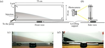
Figure 6. A sketch of the experimental rectangular channel. (a) Front view, (b) side view, (c) a snapshot of the channel during experiment B1 (the shaded area is the advancing current) and (d) a snapshot of the channel filled with glass beads during experiment A1 (the dark area is the advancing current and the grey area is the porous medium not yet reached by the current).
The HB fluids were obtained by mixing deionized water, Carbopol 980 (0.05 %–0.14 %) and ink, with subsequent neutralization by adding NaOH. The mass density was measured with a hydrometer (STV3500/23, Salmoiraghi) or a pycnometer, with an accuracy of 1 %.
The rheologic behaviour of the fluid was analysed in a parallel-plate rheometer (dynamic shear rheometer, Anton Paar Physica MCR 101), conducting several different tests, both static and dynamic, to evaluate the fluid behaviour index, the consistency index and the yield stress. When dealing with non-Newtonian fluids, either Ostwald–de Waele (power law) or HB, the characterization of the correct parameters representing the rheological behaviour of the fluid can be challenging. However, the final aim of the experiments is clear, and that is to verify the proposed model by using independent measurements of both the flow field characteristics (front position and current thickness over time) and the fluid rheometric parameters. It is noteworthy that the models used to describe the fluid rheology and obtain the rheometric parameters do not have a general validity but are an approximation of the fluid behaviour in a limited shear range. Furthermore, none of the flow fields generated in the measuring instruments (mainly rheometers) are perfectly viscometric. The problem of correctly estimating the rheometric parameters is particularly significant for HB fluids, for which yield stress estimation (and definition) is far from trivial. See the review paper by Nguyen & Boger (Reference Nguyen and Boger1992) for a discussion on the topic and a description of the methodology adopted in our laboratory experiments. Therefore, in order to evaluate the accuracy of the measurements of the yield stress, we carried out numerous additional experiments with different methods, broadly classified as ‘direct’ and ‘indirect’ methods; see the further description in appendix A.
The glass beads forming the porous medium had nominal diameters of 3, 4 and 5 mm $\pm 0.1~\text{mm}$
, depending on the test. The profile of the current was detected with either a stills camera (Canon EOS 3D,
$\pm 0.1~\text{mm}$
, depending on the test. The profile of the current was detected with either a stills camera (Canon EOS 3D, $3456\times 2304$
pixels) operating at a rate of
$3456\times 2304$
pixels) operating at a rate of $0.5~\text{frames}\,\text{s}^{-1}$
or a high-resolution video camera (Canon Legria,
$0.5~\text{frames}\,\text{s}^{-1}$
or a high-resolution video camera (Canon Legria, $1920\times 1080$
pixels) operating at
$1920\times 1080$
pixels) operating at $25~\text{frames}\,\text{s}^{-1}$
. The images were then postprocessed with a proprietary software package in order to be referenced to a laboratory coordinate system and for the boundary between the (dark) intruding current and the empty cell or the (light) porous medium to be extracted and parameterized. With this set-up, the overall accuracy in detecting the profile of the current was approximately 1 mm, while the uncertainty in measuring timings was negligible. During all experiments, the natural packing prevented any movement of the beads, as demonstrated by the images used for extracting the fluid interface.
$25~\text{frames}\,\text{s}^{-1}$
. The images were then postprocessed with a proprietary software package in order to be referenced to a laboratory coordinate system and for the boundary between the (dark) intruding current and the empty cell or the (light) porous medium to be extracted and parameterized. With this set-up, the overall accuracy in detecting the profile of the current was approximately 1 mm, while the uncertainty in measuring timings was negligible. During all experiments, the natural packing prevented any movement of the beads, as demonstrated by the images used for extracting the fluid interface.
Tables 1 and 2 list the parameters for the two sets of experiments (fracture and 2D porous medium) and four series with increasing concentration of Carbopol (labelled from A to D, corresponding to $0.05\,\%$
,
$0.05\,\%$
, $0.08\,\%$
,
$0.08\,\%$
, $0.10\,\%$
and
$0.10\,\%$
and $0.14\,\%$
concentration respectively). Figure 7(a) shows the dimensionless front position of the currents versus time for 13 tests conducted in the fracture with three different HB fluids. The plotting variables have been chosen to collapse all of the experimental data into a single line. In order to separate the results for the three different fluids, the experimental front position was multiplied by 0.5 and 1.5 for experiments A and C respectively. The uncertainty in the model and experimental data was computed following the same procedure as reported in Di Federico et al. (Reference Di Federico, Longo, Chiapponi, Archetti and Ciriello2014), and is represented by the dashed lines and error bars corresponding to plus or minus one standard deviation (STD) for the data. The front propagation is generally linear for all tests, with some discrepancy at early times due to the effects of the injection geometry and the poor adherence of the experiments to model assumptions. We recall that the solution is an ‘intermediate asymptotic’ to the general solution, and is valid for times and distances from the boundaries large enough to forget the details of the boundary (or initial) conditions but far enough from the ultimate asymptotic state of the system. Hence, we expect that also for longer time the experimental results will deviate from the self-similar solution.
$0.14\,\%$
concentration respectively). Figure 7(a) shows the dimensionless front position of the currents versus time for 13 tests conducted in the fracture with three different HB fluids. The plotting variables have been chosen to collapse all of the experimental data into a single line. In order to separate the results for the three different fluids, the experimental front position was multiplied by 0.5 and 1.5 for experiments A and C respectively. The uncertainty in the model and experimental data was computed following the same procedure as reported in Di Federico et al. (Reference Di Federico, Longo, Chiapponi, Archetti and Ciriello2014), and is represented by the dashed lines and error bars corresponding to plus or minus one standard deviation (STD) for the data. The front propagation is generally linear for all tests, with some discrepancy at early times due to the effects of the injection geometry and the poor adherence of the experiments to model assumptions. We recall that the solution is an ‘intermediate asymptotic’ to the general solution, and is valid for times and distances from the boundaries large enough to forget the details of the boundary (or initial) conditions but far enough from the ultimate asymptotic state of the system. Hence, we expect that also for longer time the experimental results will deviate from the self-similar solution.
Table 1. Parameters for the experiments in the fracture. The injected volume scales with $t^{2}$
.
$t^{2}$
.
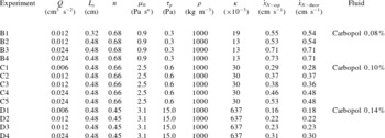
Table 2. Parameters of the experiments in a porous medium, with volume $\propto t^{\unicode[STIX]{x1D6FC}}$
. The experimental and theoretical front speed is not constant for the last four experiments.
$\propto t^{\unicode[STIX]{x1D6FC}}$
. The experimental and theoretical front speed is not constant for the last four experiments.
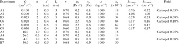
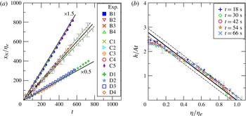
Figure 7. A comparison of theory with experiments for the fracture. (a) The front position $x_{N}/\unicode[STIX]{x1D702}_{e}$
as a function of dimensionless time
$x_{N}/\unicode[STIX]{x1D702}_{e}$
as a function of dimensionless time $t$
for all tests. The three bold lines represent the perfect agreement with theory for the three different fluids used in the experiments. (b) The dimensionless profile of the current at different times for experiment B3. The error bars refer to the profile at
$t$
for all tests. The three bold lines represent the perfect agreement with theory for the three different fluids used in the experiments. (b) The dimensionless profile of the current at different times for experiment B3. The error bars refer to the profile at $t=66~\text{s}$
and correspond to
$t=66~\text{s}$
and correspond to $\pm$
one STD, the bold straight line indicates the theoretical profiles and the dashed lines are the confidence limits of the model. For clarity, in both (a) and (b), one point of every three is plotted.
$\pm$
one STD, the bold straight line indicates the theoretical profiles and the dashed lines are the confidence limits of the model. For clarity, in both (a) and (b), one point of every three is plotted.
Figure 7(b) shows the shape of the current at different times for experiment B3. The normalized profiles show a fairly good collapse to a single curve, even though the discrepancy between experiments and theory becomes evident for $\unicode[STIX]{x1D702}/\unicode[STIX]{x1D702}_{e}<0.30$
and near the front. This is due to the disturbances at the inlet (the inflow is located near the bottom in the experiments, while it is assumed to be evenly distributed along the vertical in the theory), to non-negligible vertical velocities near the inlet (see Longo & Di Federico Reference Longo and Di Federico2014) and to the bottom stress, which becomes relevant at the tip of the current. The experimental profiles are similar for all other tests.
$\unicode[STIX]{x1D702}/\unicode[STIX]{x1D702}_{e}<0.30$
and near the front. This is due to the disturbances at the inlet (the inflow is located near the bottom in the experiments, while it is assumed to be evenly distributed along the vertical in the theory), to non-negligible vertical velocities near the inlet (see Longo & Di Federico Reference Longo and Di Federico2014) and to the bottom stress, which becomes relevant at the tip of the current. The experimental profiles are similar for all other tests.
Figure 8(a) shows the front position for the six experiments conducted in a porous medium with three different HB fluids. The profile was corrected for capillary effects following the procedure outlined in Longo et al. (Reference Longo, Di Federico, Chiapponi and Archetti2013b
). The front velocity shows a fairly good agreement with the theoretical constant velocity, even though asymptotically there are larger discrepancies due to the geometry of the current, with a very thin nose affected by the bottom boundary effects. The experimental profiles of the current at different times are shown in figure 8(b) for experiment A2. The profiles collapse to a single curve, which is significantly affected by the disturbances at the inlet. The experimental points are within the confidence limits of the theoretical models and show a clear linearity for $\unicode[STIX]{x1D702}>0.5\unicode[STIX]{x1D702}_{ep}$
. In order to also check the model for the asymptotic solution with
$\unicode[STIX]{x1D702}>0.5\unicode[STIX]{x1D702}_{ep}$
. In order to also check the model for the asymptotic solution with $\unicode[STIX]{x1D6FC}\neq 2$
, some experiments were designed for constant (
$\unicode[STIX]{x1D6FC}\neq 2$
, some experiments were designed for constant ( $\unicode[STIX]{x1D6FC}=1$
) and waning (
$\unicode[STIX]{x1D6FC}=1$
) and waning ( $\unicode[STIX]{x1D6FC}=0.6$
) inflow rate, with two different HB fluids and three different bead diameters (see the last four experiments in table 2). Figure 9 shows the experimental front position (symbols) and the first-order expansion of the self-similar solution (solid curves). The overlap in each case is satisfactory, in particular for experiments at constant inflow rate.
$\unicode[STIX]{x1D6FC}=0.6$
) inflow rate, with two different HB fluids and three different bead diameters (see the last four experiments in table 2). Figure 9 shows the experimental front position (symbols) and the first-order expansion of the self-similar solution (solid curves). The overlap in each case is satisfactory, in particular for experiments at constant inflow rate.
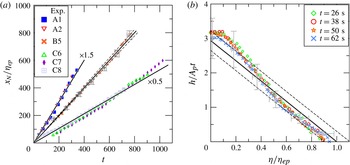
Figure 8. A comparison of theory with experiments for 2D porous flow (rectangular channel filled with glass beads). For caption, see figure 7. (b) Refers to experiment A2.

Figure 9. A comparison of theory (solid curves) with experiments (symbols) for the 2D porous medium, showing $x_{N}$
as a function of dimensionless time
$x_{N}$
as a function of dimensionless time $t$
for all tests. The injected volume scales with
$t$
for all tests. The injected volume scales with $t^{\unicode[STIX]{x1D6FC}}$
. The experimental parameters are listed in table 2.
$t^{\unicode[STIX]{x1D6FC}}$
. The experimental parameters are listed in table 2.
6 Conclusions
A general model was developed for gravity-driven flows of HB fluids in a narrow fracture or 2D porous medium, extending existing formulations for Newtonian and power-law fluids. For the special case of an inflow rate linearly time-increasing, a self-similar solution was derived for both cases: the front of the current advances at constant speed and with a linear profile. For the general case of a power-law inflow rate, an expansion of the self-similar solution valid for an Ostwald–de Waele fluid was developed, in the limit $\unicode[STIX]{x1D705}\ll 1$
or
$\unicode[STIX]{x1D705}\ll 1$
or $\unicode[STIX]{x1D705}_{p}\ll 1$
, with these two parameters marking the deviation from pure power-law behaviour. The expansion has a validity controlled by the value of
$\unicode[STIX]{x1D705}_{p}\ll 1$
, with these two parameters marking the deviation from pure power-law behaviour. The expansion has a validity controlled by the value of $\unicode[STIX]{x1D6FC}$
; hence, it is valid within a time interval limited by a critical time value beyond which either the approximation in deriving the differential equation or the adopted expansion become invalid.
$\unicode[STIX]{x1D6FC}$
; hence, it is valid within a time interval limited by a critical time value beyond which either the approximation in deriving the differential equation or the adopted expansion become invalid.
The rheological parameters of the HB fluids have been measured with independent tests, with two different rheometers and with both direct and indirect methods for the yield stress. The results for the yield stress vary according to the different methods adopted. However, a single value of the yield stress (the lowest in the list of measured values) has proven to correctly characterize all of the experiments performed with the same fluid in the Hele-Shaw cell and in the porous medium.
The experiments were mostly conducted with volume scaling in time as $\unicode[STIX]{x1D6FC}=2$
, with some additional experiments conducted with
$\unicode[STIX]{x1D6FC}=2$
, with some additional experiments conducted with $\unicode[STIX]{x1D6FC}=0.6,1$
. Each test shows reasonable agreement with the theory for flow in fractures and porous media, especially so for the former. Deviations from the linear profile forecast for
$\unicode[STIX]{x1D6FC}=0.6,1$
. Each test shows reasonable agreement with the theory for flow in fractures and porous media, especially so for the former. Deviations from the linear profile forecast for $\unicode[STIX]{x1D6FC}=2$
occur near the inlet. In the 2D porous medium, a dome develops near the inlet, followed by a profile in good agreement with the theory. In all cases, the theoretical prediction lies within the confidence limits of the experimental data. These experimental results provide a verification of the flow model for HB fluids in fractures and also a further verification of the extended Darcy law proposed by Chevalier et al. (Reference Chevalier, Chevalier, Clain, Dupla, Canou, Rodts and Coussot2013) for HB fluid flow in porous media. However, the existence of non-zero Darcy flow below the threshold pressure gradient requires further fundamental experimental investigation.
$\unicode[STIX]{x1D6FC}=2$
occur near the inlet. In the 2D porous medium, a dome develops near the inlet, followed by a profile in good agreement with the theory. In all cases, the theoretical prediction lies within the confidence limits of the experimental data. These experimental results provide a verification of the flow model for HB fluids in fractures and also a further verification of the extended Darcy law proposed by Chevalier et al. (Reference Chevalier, Chevalier, Clain, Dupla, Canou, Rodts and Coussot2013) for HB fluid flow in porous media. However, the existence of non-zero Darcy flow below the threshold pressure gradient requires further fundamental experimental investigation.
An additional promising area of research suggested by our work is the interaction of rheologically complex fluids (described, e.g., by the HB model) with spatial heterogeneity in key problem parameters, using either a deterministic or a stochastic approach. For fracture flow, heterogeneity may be represented by a spatially variable aperture (Lavrov Reference Lavrov2013), or by obstructions, local contractions and expansions (Hewitt et al. Reference Hewitt, Daneshi, Balmforth and Martinez2016). For porous medium flow, spatial variability of permeability may be modelled using deterministic trends or directly as a random field, using approaches and methods typical of stochastic hydrology. We are currently working on these problems and plan to report on our efforts in the near future.
Appendix A. Rheometry of the fluids
Most measurements were conducted with a parallel-plate rheometer (dynamic shear rheometer, Anton Paar Physica MCR 101, equipped with a moving plane plate of diameter 25 mm, with the gap equal to 1 mm in most cases) and with a strain-controlled rheometer (coaxial cylinders, Haake RT 10 RotoVisco, equipped with cup and rotor according to DIN 53019, with internal radius equal to 19.36 mm and external radius equal to 21 mm). In order to limit the slip, the surfaces of the cup and the rotor were roughened with strips of Sellotape, and the surfaces of the plates were roughened with sandpaper P-60 glued onto the smooth surfaces (see Carotenuto & Minale Reference Carotenuto and Minale2013, for an in-depth analysis of the effects of sandpaper on rheological measurements of Newtonian fluids). Additionally, in order to prevent absorption, the sandpaper was painted with transparent acrylic.
Figure 10(a) shows the classical stress strain-rate experimental results obtained with the coaxial-cylinder rheometer; figure 10(b) shows similar results for the $0.10\,\%$
fluid obtained with the parallel-plate rheometer. The continuous curves represent the HB model interpolation for the reduced series of experimental points, visualized with filled symbols. The reduction of the sample is required partly due to the limits of accuracy of the instruments at very low shear rate and partly as a consequence of the poor adaptation of the model to the real rheological behaviour of the fluid. This is the simplest and most common procedure to estimate the yield stress, but the results depend on the cutoff value of the shear rate used to select the reduced sample. For the present data,
$0.10\,\%$
fluid obtained with the parallel-plate rheometer. The continuous curves represent the HB model interpolation for the reduced series of experimental points, visualized with filled symbols. The reduction of the sample is required partly due to the limits of accuracy of the instruments at very low shear rate and partly as a consequence of the poor adaptation of the model to the real rheological behaviour of the fluid. This is the simplest and most common procedure to estimate the yield stress, but the results depend on the cutoff value of the shear rate used to select the reduced sample. For the present data, $\unicode[STIX]{x1D70F}_{p}=1.1,2.9,7\,\text{Pa}$
for measurements in the coaxial-cylinder rheometer and for fluids with increasing concentration of Carbopol. For measurements taken with the parallel-plate rheometer, the yield stress for the mixture with
$\unicode[STIX]{x1D70F}_{p}=1.1,2.9,7\,\text{Pa}$
for measurements in the coaxial-cylinder rheometer and for fluids with increasing concentration of Carbopol. For measurements taken with the parallel-plate rheometer, the yield stress for the mixture with $0.10\,\%$
of Carbopol 980 is equal to
$0.10\,\%$
of Carbopol 980 is equal to $1.3\,\text{Pa}$
. This method of estimation of the yield stress is an indirect one.
$1.3\,\text{Pa}$
. This method of estimation of the yield stress is an indirect one.
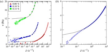
Figure 10. (a) Experimental shear-stress shear-rate curves for the three fluids Carbopol 980 0.08, 0.10 and $0.14\,\%$
, measured with the coaxial-cylinder rheometer. (b) Experimental shear-stress shear-rate curves for Carbopol 980
$0.14\,\%$
, measured with the coaxial-cylinder rheometer. (b) Experimental shear-stress shear-rate curves for Carbopol 980 $0.10\,\%$
, measured with the parallel-plate rheometer. The curves are the HB model interpolation for the reduced series of experimental points, represented by the filled symbols.
$0.10\,\%$
, measured with the parallel-plate rheometer. The curves are the HB model interpolation for the reduced series of experimental points, represented by the filled symbols.
A direct method is based on stress relaxation. The fluid is sheared, reaching a specific value of strain, then shearing stops and the shear stress required to guarantee the reached strain is recorded. Its asymptotic value is taken to be equal to the yield stress.
Figure 11(a) shows the results for various strains in the $0.10\,\%$
Carbopol 980 fluid. The asymptotic value lies in the range 0.6–1.0 Pa and is a function of the imposed strain; it decays for increasing strain since the degree of disturbances in the fluid controls the late behaviour of the system. Figure 11(b) shows the asymptotic shear stress for imposed shear rate. After an initial growth, the shear stress reaches a plateau, up to a limiting value that makes the transient state extremely long. The stress corresponding to the minimum plateau reached is assumed as an upper limit of the yield stress. For the
$0.10\,\%$
Carbopol 980 fluid. The asymptotic value lies in the range 0.6–1.0 Pa and is a function of the imposed strain; it decays for increasing strain since the degree of disturbances in the fluid controls the late behaviour of the system. Figure 11(b) shows the asymptotic shear stress for imposed shear rate. After an initial growth, the shear stress reaches a plateau, up to a limiting value that makes the transient state extremely long. The stress corresponding to the minimum plateau reached is assumed as an upper limit of the yield stress. For the $0.10\,\%$
Carbopol 980 fluid,
$0.10\,\%$
Carbopol 980 fluid, $\unicode[STIX]{x1D70F}_{min}\approx \unicode[STIX]{x1D70F}_{p}=1.15\,\text{Pa}$
.
$\unicode[STIX]{x1D70F}_{min}\approx \unicode[STIX]{x1D70F}_{p}=1.15\,\text{Pa}$
.
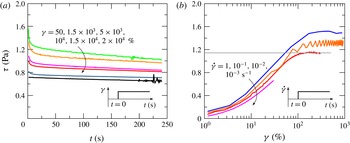
Figure 11. Carbopol 980 $0.10\,\%$
. (a) Asymptotic stress at constant strain; (b) asymptotic stress at constant strain rate. The insets show the procedure adopted in testing.
$0.10\,\%$
. (a) Asymptotic stress at constant strain; (b) asymptotic stress at constant strain rate. The insets show the procedure adopted in testing.
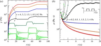
Figure 12. Creep–recovery method for the Carbopol 980 $0.10\,\%$
. (a) Strain–time curves and (b) corresponding apparent viscosity. The yield stress lies between
$0.10\,\%$
. (a) Strain–time curves and (b) corresponding apparent viscosity. The yield stress lies between $\unicode[STIX]{x1D70F}=1\,\text{Pa}$
and
$\unicode[STIX]{x1D70F}=1\,\text{Pa}$
and $\unicode[STIX]{x1D70F}=1.5\,\text{Pa}$
. Measurements were conducted with the parallel-plate rheometer; the inset shows the procedure adopted for testing.
$\unicode[STIX]{x1D70F}=1.5\,\text{Pa}$
. Measurements were conducted with the parallel-plate rheometer; the inset shows the procedure adopted for testing.
Another method is called creep and recovery. A constant shear stress is applied in steps and the creep is observed. If a more or less complete recovery is reached, then the applied stress was below the yield stress and the continuum behaved as an elastic solid. If a limited or null recovery is reached, then the applied stress was above the yield stress.
Figure 12(a) shows strain–time curves for Carbopol 980 $0.10\,\%$
, with stress imposed for 20 s (except for the curve relative to
$0.10\,\%$
, with stress imposed for 20 s (except for the curve relative to $\unicode[STIX]{x1D70F}=1\,\text{Pa}$
) and a recovery for 30 s. Figure 12(b) shows the corresponding time evolution of apparent viscosity. The residual strain is equal to
$\unicode[STIX]{x1D70F}=1\,\text{Pa}$
) and a recovery for 30 s. Figure 12(b) shows the corresponding time evolution of apparent viscosity. The residual strain is equal to $28,32,54,85\,\%$
for
$28,32,54,85\,\%$
for $\unicode[STIX]{x1D70F}=0.2,0.5,1,1.5~\text{Pa}$
respectively, and the yield stress is assumed to be in the range
$\unicode[STIX]{x1D70F}=0.2,0.5,1,1.5~\text{Pa}$
respectively, and the yield stress is assumed to be in the range $[1{-}1.5]~\text{Pa}$
. The estimation is affected by a significant uncertainty, because in the present experiments the residual deformation is monotonic with the imposed stress and no abrupt increase is observed. For other fluids, the behaviour is much sharper (Magnin & Piau Reference Magnin and Piau1987).
$[1{-}1.5]~\text{Pa}$
. The estimation is affected by a significant uncertainty, because in the present experiments the residual deformation is monotonic with the imposed stress and no abrupt increase is observed. For other fluids, the behaviour is much sharper (Magnin & Piau Reference Magnin and Piau1987).
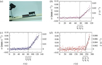
Figure 13. (a) A photo of the inclined plane and of the accessories used for a direct measurement of the yield stress. The electronic level and the video camera are in the same frame of the fluid layer. (b–d) The plots of the free surface velocity versus time for (b) a mixture of Carbopol 980 ( $0.08\,\%$
neutralized), (c) a mixture of Carbopol 980 (
$0.08\,\%$
neutralized), (c) a mixture of Carbopol 980 ( $0.10\,\%$
neutralized) and (d) a mixture of Carbopol 980 (
$0.10\,\%$
neutralized) and (d) a mixture of Carbopol 980 ( $0.14\,\%$
neutralized). The solid lines indicate the fitted free surface velocity; the vertical solid line indicates the assumed start of flow motion. The secondary horizontal axis indicates the angle with respect to the horizontal; the secondary vertical axis indicates the average shear rate obtained by dividing the free surface velocity and the starting thickness of the layer, neglecting its reduction in time. The thickness of the layer was set to 0.3, 0.3 and 1 cm for Carbopol 980 0.08, 0.10 and
$0.14\,\%$
neutralized). The solid lines indicate the fitted free surface velocity; the vertical solid line indicates the assumed start of flow motion. The secondary horizontal axis indicates the angle with respect to the horizontal; the secondary vertical axis indicates the average shear rate obtained by dividing the free surface velocity and the starting thickness of the layer, neglecting its reduction in time. The thickness of the layer was set to 0.3, 0.3 and 1 cm for Carbopol 980 0.08, 0.10 and $0.14\,\%$
respectively.
$0.14\,\%$
respectively.
The yield stress was also measured with a direct method based on the static stability of a layer of fluid on an inclined plane (Uhlherr et al. Reference Uhlherr, Park, Tiu and Andrews1984), by adopting the same device and experimental technique as detailed in Longo et al. (Reference Longo, Chiapponi and Di Federico2016). The yield stress can be evaluated by assuming that in the incipient motion the following balance holds:
 $$\begin{eqnarray}\unicode[STIX]{x1D70F}_{p}=\unicode[STIX]{x1D70C}gh\sin \unicode[STIX]{x1D703}_{c},\end{eqnarray}$$
where $h$
is the thickness of the layer and
$h$
is the thickness of the layer and $\unicode[STIX]{x1D703}_{c}$
is the critical angle.
$\unicode[STIX]{x1D703}_{c}$
is the critical angle.
The incipient motion of the free surface, as detected with a particle image velocity algorithm applied to the images recorded by a video camera, is assumed as an indicator of the sliding. Figure 13 shows, for three different yield stress fluids, the experimental apparatus and the plots of the free surface for increasing bottom inclination. The dots represent the average velocity of the free surface, with dispersion due to vibrations and to noise in the images. It is possible to detect a kink, enhanced by separately interpolating the premotion and the postmotion experimental data with two different straight lines. However, a creep motion is detected near the critical angle, presumably due to the elastic deformation of the layer of material before flowing.
The overall uncertainty, computed as
 $$\begin{eqnarray}{\displaystyle \frac{\text{d}\unicode[STIX]{x1D70F}_{p}}{\unicode[STIX]{x1D70F}_{p}}}={\displaystyle \frac{\text{d}\unicode[STIX]{x1D70C}}{\unicode[STIX]{x1D70C}}}+{\displaystyle \frac{\text{d}h}{h}}+{\displaystyle \frac{\text{d}\unicode[STIX]{x1D703}_{c}}{\tan \unicode[STIX]{x1D703}_{c}}},\end{eqnarray}$$
has a significant contribution due to the uncertainty in the thickness of the layer $h$
. By assuming that the critical angle is detected within the uncertainty of the electronic level (
$h$
. By assuming that the critical angle is detected within the uncertainty of the electronic level ( $\pm 0.1^{\circ }$
), and assuming an uncertainty in the thickness measurements equal to
$\pm 0.1^{\circ }$
), and assuming an uncertainty in the thickness measurements equal to $\pm 0.3\,\text{cm}$
, the estimated yield stress values are
$\pm 0.3\,\text{cm}$
, the estimated yield stress values are $\unicode[STIX]{x1D70F}_{p}=1.0\pm 0.1\,\text{Pa}$
,
$\unicode[STIX]{x1D70F}_{p}=1.0\pm 0.1\,\text{Pa}$
, $\unicode[STIX]{x1D70F}_{p}=1.2\pm 0.2\,\text{Pa}$
,
$\unicode[STIX]{x1D70F}_{p}=1.2\pm 0.2\,\text{Pa}$
, $\unicode[STIX]{x1D70F}_{p}=26\pm 1\,\text{Pa}$
for Carbopol 980
$\unicode[STIX]{x1D70F}_{p}=26\pm 1\,\text{Pa}$
for Carbopol 980 $0.08,0.10,0.14\,\%$
respectively. However, the true uncertainty is larger than our estimate, due to the intrinsic uncertainty in the definition of the critical angle.
$0.08,0.10,0.14\,\%$
respectively. However, the true uncertainty is larger than our estimate, due to the intrinsic uncertainty in the definition of the critical angle.
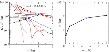
Figure 14. (a) Evolution of the storage modulus $G^{\prime }$
(red dashed lines) and the loss modulus
$G^{\prime }$
(red dashed lines) and the loss modulus $G^{\prime \prime }$
(grey continuous lines) for the
$G^{\prime \prime }$
(grey continuous lines) for the $0.10\,\%$
Carbopol 980 mixture as a function of stress for different frequencies. The symbols are the intersection between the moduli (cross-over), conventionally representing the flow point. (b) Cross-over stress as a function of the frequency. Measurements with parallel-plate rheometer, gap 1 mm,
$0.10\,\%$
Carbopol 980 mixture as a function of stress for different frequencies. The symbols are the intersection between the moduli (cross-over), conventionally representing the flow point. (b) Cross-over stress as a function of the frequency. Measurements with parallel-plate rheometer, gap 1 mm, $T=298\,\text{K}$
.
$T=298\,\text{K}$
.
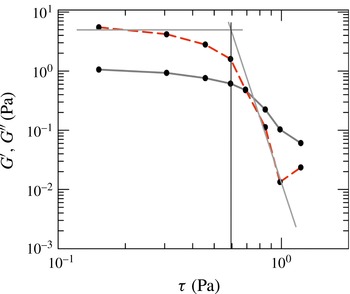
Figure 15. Sweep experiments with Carbopol 980 $0.10\,\%$
at a frequency of
$0.10\,\%$
at a frequency of $\unicode[STIX]{x1D714}=0.1\,\text{Hz}$
. The yield stress is evaluated as the abscissa of the intersection of the two straight lines interpolating the storage modulus
$\unicode[STIX]{x1D714}=0.1\,\text{Hz}$
. The yield stress is evaluated as the abscissa of the intersection of the two straight lines interpolating the storage modulus $G^{\prime }$
on the left and right sides of the cross-over.
$G^{\prime }$
on the left and right sides of the cross-over.
Another method to estimate the yield stress is based on the dynamic behaviour at small deformation, as detected with oscillatory shear tests, with the measurement of the storage modulus $G^{\prime }(\unicode[STIX]{x1D714})$
and the loss modulus
$G^{\prime }(\unicode[STIX]{x1D714})$
and the loss modulus $G^{\prime \prime }(\unicode[STIX]{x1D714})$
, representative of the elastic and the viscous behaviour of the continuum respectively. Applying a sinusoidal strain
$G^{\prime \prime }(\unicode[STIX]{x1D714})$
, representative of the elastic and the viscous behaviour of the continuum respectively. Applying a sinusoidal strain $\unicode[STIX]{x1D6FE}=\unicode[STIX]{x1D6FE}_{0}\sin \unicode[STIX]{x1D714}t$
with small amplitude
$\unicode[STIX]{x1D6FE}=\unicode[STIX]{x1D6FE}_{0}\sin \unicode[STIX]{x1D714}t$
with small amplitude $\unicode[STIX]{x1D6FE}_{0}$
and frequency
$\unicode[STIX]{x1D6FE}_{0}$
and frequency $\unicode[STIX]{x1D714}$
, the time varying stress
$\unicode[STIX]{x1D714}$
, the time varying stress $\unicode[STIX]{x1D70F}=\unicode[STIX]{x1D70F}_{0}\sin (\unicode[STIX]{x1D714}+\unicode[STIX]{x1D6FF}t)$
is measured, where
$\unicode[STIX]{x1D70F}=\unicode[STIX]{x1D70F}_{0}\sin (\unicode[STIX]{x1D714}+\unicode[STIX]{x1D6FF}t)$
is measured, where $\unicode[STIX]{x1D6FF}$
is a phase shift. The complex modulus
$\unicode[STIX]{x1D6FF}$
is a phase shift. The complex modulus $G^{\ast }(\unicode[STIX]{x1D714})\equiv \unicode[STIX]{x1D70F}/\unicode[STIX]{x1D6FE}=G^{\prime }(\unicode[STIX]{x1D714})+iG^{\prime \prime }(\unicode[STIX]{x1D714})$
has the two components
$G^{\ast }(\unicode[STIX]{x1D714})\equiv \unicode[STIX]{x1D70F}/\unicode[STIX]{x1D6FE}=G^{\prime }(\unicode[STIX]{x1D714})+iG^{\prime \prime }(\unicode[STIX]{x1D714})$
has the two components $G^{\prime }$
and
$G^{\prime }$
and $G^{\prime \prime }$
, representative of elasticity (perfect if
$G^{\prime \prime }$
, representative of elasticity (perfect if $G^{\prime \prime }=0,\unicode[STIX]{x1D6FF}=0$
) and viscosity (perfect if
$G^{\prime \prime }=0,\unicode[STIX]{x1D6FF}=0$
) and viscosity (perfect if $G^{\prime }=0,\unicode[STIX]{x1D6FF}=90^{\circ }$
) respectively. The yield stress can be estimated as the intercept of the tangent of the storage modulus considering the domains before and after the cross-over (De Graef et al.
Reference De Graef, Depypere, Minnaert and Dewettinck2011). Figure 14(a) shows the moduli measured at different frequencies for Carbopol 980
$G^{\prime }=0,\unicode[STIX]{x1D6FF}=90^{\circ }$
) respectively. The yield stress can be estimated as the intercept of the tangent of the storage modulus considering the domains before and after the cross-over (De Graef et al.
Reference De Graef, Depypere, Minnaert and Dewettinck2011). Figure 14(a) shows the moduli measured at different frequencies for Carbopol 980 $0.10\,\%$
, while figure 14(b) shows the cross-over variation with the frequency
$0.10\,\%$
, while figure 14(b) shows the cross-over variation with the frequency $\unicode[STIX]{x1D714}$
. Selecting the lowest frequency measurements (
$\unicode[STIX]{x1D714}$
. Selecting the lowest frequency measurements ( $\unicode[STIX]{x1D714}=0.1\,\text{s}^{-1}$
), the yield stress can be estimated as shown in figure 15, obtaining
$\unicode[STIX]{x1D714}=0.1\,\text{s}^{-1}$
), the yield stress can be estimated as shown in figure 15, obtaining $\unicode[STIX]{x1D70F}_{y}\approx 0.6\,\text{Pa}$
.
$\unicode[STIX]{x1D70F}_{y}\approx 0.6\,\text{Pa}$
.
Table 3 lists the estimated yield stress adopting the different techniques for the $0.10\,\%$
Carbopol 980 fluid. The results indicate the dispersion of the data and that measurements can give at most a range of variation of the yield stress to be used for the verification of the theoretical models.
$0.10\,\%$
Carbopol 980 fluid. The results indicate the dispersion of the data and that measurements can give at most a range of variation of the yield stress to be used for the verification of the theoretical models.
Table 3. Synthesis of the yield stress estimations for Carbopol 980 $0.10\,\%$
. Rheom. 1 refers to the coaxial-cylinder rheometer, while rheom. 2 refers to the parallel-plate rheometer.
$0.10\,\%$
. Rheom. 1 refers to the coaxial-cylinder rheometer, while rheom. 2 refers to the parallel-plate rheometer.