


1. Introduction
Natural convection under the influence rotation occurs widely in many geo- and astrophyiscal environments (Chen & Guo Reference Chen and Guo2003; King et al. Reference King, Stellmach, Noir, Hansen and Aurnou2009; Cheng et al. Reference Cheng, Stellmach, Ribeiro, Grannan, King and Aurnou2015, Reference Cheng, Aurnou, Julien and Kunnen2018; Plumley & Julien Reference Plumley and Julien2019). For example, the large-scale vortices observed in the giant planets, such as the ‘Great Red Spot’ at the atmosphere of Jupiter, are sustained by convection under a strong Coriolis force (Guervilly, Hughes & Jones Reference Guervilly, Hughes and Jones2014; Favier, Guervilly & Knobloch Reference Favier, Guervilly and Knobloch2019; Cai Reference Cai2021). Moreover, moist convection is considered an important factor in explaining the formation of a polar vortex in giant planets (O'Neill, Emanuel & Flierl Reference O'Neill, Emanuel and Flierl2015) and the upscale energy transfer strengthening the large cyclones at Jovian high latitudes (Siegelman et al. Reference Siegelman2022). Understanding the dynamics of these systems relies deeply on the observations. However, owing to the difficulty in data acquisition and the complexity of these systems, idealized models are very useful complementary approaches used to investigate the dynamics of these systems. A classical physical model for rotating convection is the rotating Rayleigh–Bénard convection (RBC). When the system is rapidly rotating, the horizontal pressure gradient is balanced by the Coriolis force at the leading order, which is known as the geostrophic balance. Rayleigh–Bénard convection under geostrophic balance possesses features relevant to many important issues of the geo- and astrophysical systems, thus, it has attracted considerable interest in recent decades (Knobloch Reference Knobloch1998; King et al. Reference King, Stellmach, Noir, Hansen and Aurnou2009; Stevens et al. Reference Stevens, Zhong, Clercx, Ahlers and Lohse2009; Zhong et al. Reference Zhong, Stevens, Clercx, Verzicco, Lohse and Ahlers2009; Weiss et al. Reference Weiss, Stevens, Zhong, Clercx, Lohse and Ahlers2010; King, Stellmach & Aurnou Reference King, Stellmach and Aurnou2012; Ecke & Niemela Reference Ecke and Niemela2014; Stellmach et al. Reference Stellmach, Lischper, Julien, Vasil, Cheng, Ribeiro, King and Aurnou2014; Kunnen Reference Kunnen2021). In this system, the rotation rate can be characterized by the Ekman number  $Ek\equiv \nu /(2\varOmega H^2)$, and the strength of buoyancy forcing is represented by the Rayleigh number $Ra\equiv (\alpha g\Delta H^3)/(\kappa \nu )$. Here $\alpha$ is the thermal expansion coefficient of the fluid, $g$ is the gravitational acceleration, $\varDelta =T_{hot}-T_{cold}$ is the temperature difference between the hot and cold plates, $H$ is the height of convection cell, $\nu$ is the kinetic viscosity, $\kappa$ is the thermal diffusivity and $\varOmega$ is the rotating rate. Rotation suppresses the vertical fluid motions as a result of the Taylor–Proudman constraint. For a laterally unlimited domain, bulk convection emerges when $Ra$ is beyond the onset Rayleigh number $Ra_c$ (Niiler & Bisshopp Reference Niiler and Bisshopp1965)
 \begin{equation} Ra_c=(8.7-9.63Ek^{1/6})Ek^{{-}4/3}. \end{equation}
For the systems with lateral boundaries, however, distinct flow structures can be found in the region adjacent to the sidewalls. These structures are called wall mode, which is azimuthally periodic and precesses in the retrograde direction (Zhong, Ecke & Steinberg Reference Zhong, Ecke and Steinberg1991; Ecke, Zhong & Knobloch Reference Ecke, Zhong and Knobloch1992; Favier & Knobloch Reference Favier and Knobloch2020). Different from the direction of precession, the mean azimuthal velocity of the outer part of the wall mode is positive (prograde). For a cylindrical system with non-slip boundaries, the onset Rayleigh number of the wall mode is given by (Zhang & Liao Reference Zhang and Liao2009)
 \begin{equation} Ra_w={\rm \pi}^2\sqrt{6\sqrt{3}}Ek^{{-}1}+46.6Ek^{{-}2/3}. \end{equation}
For a large  $Pr$ number, the wall mode emerges at a smaller $Ra$ than the bulk convection. When the bulk flow emerges, the wall-localized flow structure is also understood as the boundary zonal flow (Zhang et al. Reference Zhang, van Gils, Horn, Wedi, Zwirner, Ahlers, Ecke, Weiss, Bodenschatz and Shishkina2019; Zhang, Ecke & Shishkina Reference Zhang, Ecke and Shishkina2021; Ecke, Zhang & Shishkina Reference Ecke, Zhang and Shishkina2021; Wedi et al. Reference Wedi, Moturi, Funfschilling and Weiss2022). To avoid confusion, hereafter we refer to this flow structure adjacent to the sidewall as the boundary flow, whether or not the bulk convection sets in.
Among the various topics in geostrophic RBC, determination of the scaling relationship of heat transport efficiency is one of the key issues. This is not only attributed to the fact that heat transport itself is crucial in many physical problems, heat transport may also reflect the transition in flow morphology and the dominating force balance in the system. For this reason, the scaling relationship of the heat transport efficiency can help one to better understand the essential physics of the system, which may also enable simplification of the physical models or parameterization of the main physical quantities of the system. Moreover, the scaling relationship of heat transport efficiency provides the possibility to estimate the physical quantities or explain the features of the geo- and astrophysical environments that are beyond the achievable parameter range in experiments or simulations. The heat transport efficiency is quantified by the Nusselt number  $Nu\equiv (\langle u_zT-\kappa \partial T/\partial z\rangle _{x,y})/(\kappa \varDelta /H)$, where $\langle {\cdot }\rangle _{x,y}$ denotes the average over the horizontal plane. For laterally unbounded cases, a steep scaling relationship $Nu\sim (Ra/Ra_c)^3$ can be found numerically (King et al. Reference King, Stellmach and Aurnou2012; Cheng et al. Reference Cheng, Stellmach, Ribeiro, Grannan, King and Aurnou2015). However, recent experiments and numerical simulations using cylindrical cells observed much smaller scaling exponents than 3 (Lu et al. Reference Lu, Ding, Shi, Xia and Zhong2021). Such a difference suggests that the boundary flow has a distinct $Ra$ dependence of the heat transport efficiency from the bulk. In practical situations, the existence of lateral boundaries is inevitable. Moreover, in order to reach the geostrophic regime, many experiments are chasing for even smaller $Ek$ and higher $Ra$. One can enhance $Ra$ by using the so-called annular centrifugal Rayleigh–Bénard convection (ACRBC) system through the generation of supergravity induced by rapid rotation and the strong centrifugal force (Jiang et al. Reference Jiang, Zhu, Wang, Huisman and Sun2020; Wang et al. Reference Wang, Liu, Zhou and Sun2022), or simply by increasing the system height $H$. However, for the ACRBC system, the rotating axis is perpendicular to the effective gravity (centrifugal force), which is different from the rotating RBC system (rotating axis is parallel to the gravity). Thus, increasing $H$ is a more reasonable method to increase $Ra$ in a rotating RBC system. On the other hand, increasing $H$ or the rotation rate $\varOmega$ can both effectively extend the lower limit of the achievable $Ek$, but for the latter, the centrifugal effect could be strong so that the flow structures are significantly changed (Horn & Aurnou Reference Horn and Aurnou2018; Hu et al. Reference Hu, Huang, Xie and Xia2021; Hu, Xie & Xia Reference Hu, Xie and Xia2022; Hu & Xia Reference Hu and Xia2023). For this reason, in a rotating RBC system, it is believed to be advantageous to extend the parameter range by utilizing slender cells with a large system height (Cheng et al. Reference Cheng, Stellmach, Ribeiro, Grannan, King and Aurnou2015, Reference Cheng, Madonia, Aguirre Guzmán and Kunnen2020; de Wit et al. Reference de Wit, Aguirre Guzmán, Madonia, Cheng, Clercx and Kunnen2020). In this case, the influence of boundary flows can be significant. Thus, it is crucial to quantitatively understand the influence of boundary flow, so that one can assess and even extract the contributions of the boundary flow from the total heat flux.
In this study we use direct numerical simulations (DNS) to investigate rotating RBC in cylindrical cells with various aspect ratios, aiming to obtain a systematic understanding of the heat transport in rotating RBC in the presence of the boundary flows. To achieve this objective, we examine the bulk and boundary flows separately. The remainder of this paper is organized as follows. In § 2.1 we briefly introduce the numerical method used in this study. In § 2.2 we explain how the bulk and boundary flows are decomposed in our study, and demonstrate the reliability of our method. In §§ 3.1 and 3.2 we discuss the heat transport efficiency of the bulk and boundary flows separately. In § 3.3 we report a sharp transition in flow morphology, which is manifested as the collapse of coherency of the boundary flow structure and accompanied with a sudden drop in heat transport efficiency associated with the boundary flow. In § 3.4 we take a whole-system approach and provide a unifying understanding of the global heat transport efficiency.
2. Methodology
2.1. Numerical set-up
We consider a rotating cylindrical RBC cell with an upward rotational vector. The top and bottom plates are non-slip and with constant temperature  $T_{cold}$ and $T_{hot}$, respectively. The sidewall is non-slip and adiabatic. The geometrical property of the cell is described by the aspect ratio $\varGamma =D/H$, where $D$ is the diameter of the convection cell. This system is governed by the three-dimensional Navier–Stokes equations with Oberbeck–Boussinesq approximation. Since the centrifugal effect is usually unavoidable in many of the rapid rotating experiments, we have conducted a series of simulations that consider the centrifugal effect to examine the influence of centrifugal force. The centrifugal force is quantified by the Froude number $Fr\equiv (R\varOmega ^2)/g$, which is the ratio of centrifugal acceleration over the gravitational one. Here $R\equiv D/2$ is the radius of the cell. Length, velocity, time and temperature are respectively non-dimensionalized by the height of the convection cell $x_{ref}=H$, the convective free-fall velocity $u_{ref}=(\alpha gH\varDelta )^{1/2}$, the free-fall time $t_{ref}=x_{ref}/u_{ref}$ and the temperature difference between the hot and cold plates $T_{ref}=\varDelta$. The dimensionless governing equations with centrifugal effect are
 \begin{gather} \frac{\partial \boldsymbol{u}}{\partial t}+\boldsymbol{u}\boldsymbol{\cdot}\boldsymbol{\nabla}\boldsymbol{u}={-}\boldsymbol{\nabla} p+\sqrt{\frac{Pr}{Ra}}\nabla^2\boldsymbol{u}-\frac{1}{Ek}\sqrt{\frac{Pr}{Ra}}\hat{e}_z\times\boldsymbol{u}+\theta \hat{e}_z-Fr\frac{2r}{\varGamma}\theta\hat{e}_r, \end{gather}
 \begin{gather}\frac{\partial \theta}{\partial t}+\boldsymbol{u}\boldsymbol{\cdot}\boldsymbol{\nabla} \theta=\frac{1}{\sqrt{RaPr}}\nabla^2\theta, \end{gather}
 \begin{gather}\boldsymbol{\nabla}\boldsymbol{\cdot}\boldsymbol{u}=0. \end{gather}
Here  $Pr\equiv \nu /\kappa$ is the Prandtl number, which is the ratio between momentum and thermal diffusivity of the working fluid. All our simulations are done at $Pr=4.38$ (corresponding to water at about ${40}\,^{\circ }{\rm C}$). The dimensionless temperature variation $\theta$ is defined as $\theta \equiv (T-T_m)/\varDelta$, where $T_m\equiv (T_{hot}+T_{cold})/2$. For the sake of simplicity, symbols without special notation stand for the non-dimensional quantities in the rest of this paper.
The governing equations are solved in the cylindrical coordinates using a well-tested DNS code called CUPS, which is a fully parallelized DNS code based on the finite volume method with fourth-order precision (Kaczorowski & Xia Reference Kaczorowski and Xia2013; Kaczorowski, Chong & Xia Reference Kaczorowski, Chong and Xia2014; Chong, Ding & Xia Reference Chong, Ding and Xia2018). In this study we focus on the systems with  $Pr>1$, in which case the characteristic length scale of the temperature field (Bachelor length scale) is smaller than that of the velocity field (Kolmogorov length scale). In a traditional single-resolution scheme, the grid spacing is determined by Bachelor length scale, which is over-resolved for the velocity field. To improve computational efficiency without any sacrifice in precision, we used a multiple-resolution strategy. In this case, the momentum and temperature equations are solved in two grid sets. The momentum equations are solved in a coarser grid set than the temperature equation, which can still allow Batchelor and Kolmogorov length scales both being resolved. Using this algorithm, computational sources spent on the momentum solver is significantly reduced. We conducted three series of simulations: set I varies $Ra$ and fixes $Ek$ at $Ek=1.85\times 10^{-6}$; set II has similar conditions as set I, but includes the centrifugal effect; and in set III, $Ra$ is fixed at $Ra=2\times 10^{7}$ and $Ek$ is varied. Three aspect ratios ( $\varGamma$) are used in sets I and II, which are $\varGamma =0.5$, $1$ and $2$. In set III we fix $\varGamma =4$. Additionally, we also conduct a series of simulations in a cubic cell with aspect ratio 1 and lateral periodic boundaries. These simulations use the same Ekman number as sets I and II. All statistical quantities are taken over 400 convective free-fall time units and, for those with a high rotating rate, the statistical period is longer. In the main text of this paper, we focus on sets I and II with fixed $Ek$. In Appendix F the cases with fixed $Ra$ and the data of set III are discussed. Table 1 in the supplemental material available at https://doi.org/10.1017/jfm.2023.872 lists all the numerical set-ups for the simulations in this study, and the parameters for the cases in sets I and II are shown in figure 1.

Figure 1. Parameter space for the cases in set I and II. In these two data sets,  $Ek$ is fixed to be $1.85\times 10^{-6}$ and $Pr=4.38$. The black dashed and grey dot-dashed lines, respectively, correspond to $Ra=Ra_c$ and $Ra=Ra_w$.
2.2. Decomposition of bulk and boundary flows
The key to quantitatively understand the global heat transport of this system is to decompose the corresponding contributions from the bulk and the boundary flows. In previous studies the decomposition was achieved using a series of different radii as the cutoff (Ecke, Zhang & Shishkina Reference Ecke, Zhang and Shishkina2022). In this study we wish to decompose the respective contributions from these two regions according to the distinct features of these two regions. In order to develop a reliable and reasonable method for the decomposition across various situations with differing turbulence intensities, we first concentrate on the flow structures present within this system. In figure 2(a) we present the distributions of the azimuthal velocity  $\langle u_\phi \rangle _{t,\phi }$ averaged over time and the azimuthal direction for $Ra=8.71\times 10^8$. From figure 2(a) one can see flow structures with positive azimuthal velocity near the sidewall. It would be intuitive to separate the boundary flow and the bulk flow according to the zero crossing of $u_\phi$ from the outer positive part close to the sidewall to the inner negative part. However, such wall-localized boundary flow is a two-layer structure in which the outer and inner layers have opposite azimuthal velocities. Thus, using the simple zero-crossing criterion cannot extract the boundary flow in its entirety. We remark that this two-layer structure is consistent with the analytical solution of the velocity component parallel to the sidewall for the wall mode given by Herrmann & Busse (Reference Herrmann and Busse1993). Such similarity suggests the connection between the wall mode and the boundary flow. This two-layer structure can also be found in the averaged convective heat flux $\langle J_z\rangle _{t,\phi }$ shown in figure 2(c), where $J_z$ is the local convective heat flux defined as $J_z\equiv \sqrt {RaPr}u_z\theta$. We see that the region adjacent to the sidewall and with positive azimuthal velocity has positive convective heat flux; and the region next to it and with negative $u_\phi$ has negative $J_z$.

Figure 2. (a) Mean azimuthal velocity. (b) Vertical averaged r.m.s. of the azimuthal velocity  $\langle u^2_\phi \rangle ^{1/2}_{t,z,\phi }$. (c) Mean convective vertical heat flux. (d) The convective vertical heat flux averaged temporally and in the vertical and azimuthal directions $\langle J_z\rangle _{t,z,\phi }$. The insets of (b,d) show the corresponding data from $r/R=0$ to $1$, respectively. The control parameters for (a–d) are $Ra=8.71\times 10^8$, $Ek=1.85\times 10^{-6}$, $Fr=0$ and $\varGamma =1$. The dot-dashed and dashed lines in (a–d) respectively correspond to $r_{BF}$ and $r_0$. (e) Width of the boundary flow $\delta _{BF}/H$ (close symbols) and $\delta _{0}/H$ (open symbols) as a function of $Ra$. The blue dot-dashed and red dashed lines in (e) represent the best fits of the data for $\delta _{BF}$ and $\delta _0$, respectively.
To better identify the two-layer structure of the boundary flow and explain the method decomposing the bulk and the boundary flows, we present the root-mean-square (r.m.s.) value of the azimuthal velocity  $\langle u^2_\phi \rangle ^{1/2}_{t,z,\phi }$ in figure 2(b) and the mean convective heat flux $\langle J_z\rangle _{t,z,\phi }$ in figure 2(d). The subscript $\langle {\cdot }\rangle _{t,z,\phi }$ denotes the average over time and the vertical and azimuthal directions. We remark that the azimuthal component of the boundary flow is azimuthally periodic and its flow strength cannot be correctly reflected from $\langle u_\phi \rangle _{t,z,\phi }$, thus decomposing the bulk and the boundary flow according to $\langle u_\phi \rangle _{t,z,\phi }$ can be problematic especially at high $Ra$ when the bulk fluctuations are strong. For this reason, we instead use the r.m.s. $\langle u^2_\phi \rangle ^{1/2}_{t,z,\phi }$ in the bulk-boundary-flow decomposition. From the profile of $\langle u^2_\phi \rangle ^{1/2}_{t,z,\phi }$ presented in figure 2(b), one can clearly see a two-layer structure near the boundary and a bulk with a relatively weak flow strength. We fit the data near the two peaks using parabolic functions, which are shown as the red dot-dashed and blue dashed curves in figure 2(b), respectively. We fit the bulk part of $\langle u^2_\phi \rangle ^{1/2}_{t,z,\phi }$ ( $r/R<0.7$) using linear functions, which are denoted by the grey dotted lines in figure 2(b). We then define the left intersection between the parabolic fitting of the inner peak and the linear fitting as $r_{BF}$ (indicated by the red triangles), which is the edge separating the bulk and the boundary flow, as shown by the vertical black dot-dashed lines in figure 2. The blue and red shaded regions in figure 2(b,d) respectively represent the bulk and the boundary flows. We then define $r_0$ as the zero crossing of the outer parabolic fitting (indicated by the blue stars), which separates the prograde (outer) and retrograde (inner) parts of the boundary flow. As heat transport is one of the main topics of this study, we need to ensure that the method we used for the decomposition can effectively identify the different domains with distinguishing features especially in terms of the heat transfer. To examine our method, we also present the mean convective heat flux $\langle J_z\rangle _{t,z,\phi }$ and the result of the decomposition in the same plot, as shown in figure 2(d). We see that the boundary flow with distinguishable features in the convective heat flux can be properly identified, which provides certain validation for our method. More examples of the decomposition for various $Ra$ and different flow states are presented in Appendix A.
The width of the entire boundary flow  $\delta _{BF}\equiv \varGamma /2-r_{BF}$ and the outer boundary flow $\delta _{0}\equiv \varGamma /2-r_0$ can then be determined, respectively. We present the results of $\delta _{BF}$ and $\delta _0$ for sets I and II in figure 2(e). We find that the results of different $\varGamma$ collapse together for both $\delta _{BF}$ and $\delta _0$. Interestingly, it seems that $\delta _{BF}$ and $\delta _0$ exhibit similar $Ra$ dependence but only differ by a constant, which is found to be $\delta _{BF}\approx 2.7\delta _0$ in our study. Zhang et al. (Reference Zhang, Ecke and Shishkina2021) observed a scaling relationship $\delta _0\sim Ra^{1/4}$ using $Pr=0.8$. More recently, the experiments conducted by Wedi et al. (Reference Wedi, Moturi, Funfschilling and Weiss2022) suggests that for $Pr=6.55$, $\delta _0$ is insensitive to $Ra$. The numerical study conducted by Ecke et al. (Reference Ecke, Zhang and Shishkina2022) also has observed a relatively weak $Ra$ dependence of $\delta _0$, which is given by $\delta _0/H\sim (Ra-Ra_w)^{1/6}Ek^{2/3}$. We plot the black and red dashed lines respectively referring to $\delta _{BF,0}\sim Ra^{1/4}$ and $\delta _{BF,0}\sim Ra^{0}$ in figure 2(e) for comparison. For $Ra\lesssim 1\times 10^9$, both $\delta _{BF}$ and $\delta _{0}$ are insensitive to $Ra$, which agrees with $\delta _{BF,0}\sim Ra^{0}$ indicated by Wedi et al. (Reference Wedi, Moturi, Funfschilling and Weiss2022). When $Ra$ approaches to about $1\times 10^9$, $\delta _{BF}$ and $\delta _0$ slightly increases with $Ra$. Even though the data are scattered for $Ra\gtrsim 1\times 10^9$, it seems that $\delta _{BF,0}\sim Ra^{1/4}$ deviates from the data of either $\delta _{BF}$ or $\delta _0$. As pointed out by Wedi et al. (Reference Wedi, Moturi, Funfschilling and Weiss2022), the exponent of the power law for $\delta_0$ with $Ra$ could depend on $Pr$. Thus, such a discrepancy between our study and Zhang et al. (Reference Zhang, Ecke and Shishkina2021) may be attributed to the difference in Prandtl numbers. Nevertheless, for $Ra\lesssim 1\times 10^9$, it is reasonable to consider that $\delta _{BF}$ and $\delta _0$ are not sensitive to $Ra$.
$Ra$.
3. Results
3.1. Heat transport properties of the bulk
Using the criterion discussed in § 2.2, we proceed to investigate the heat transport in the bulk and boundary flows separately. We define  $Nu_{bulk}$ as the Nusselt number of the bulk
 \begin{equation} Nu_{bulk}\equiv\left\langle \sqrt{RaPr}u_z\theta-\frac{\partial\theta}{\partial z}\right\rangle_{t,z,\phi,r\leqslant r_{BF}}. \end{equation}
We plot  $Nu_{bulk}$ as a function of $Ra/Ra_c$ in figure 3(a). For comparison, we also present $Nu$ from simulations using lateral periodic boundary conditions. For $Ra$ smaller than the bulk onset $Ra_c$, all simulations yield $Nu_{bulk}=1$, meaning that heat is transferred conductively in the bulk. For $Ra>Ra_c$, steep scaling relationships can be observed for all cases. The periodic results can be described by $Nu\sim Ra^{3.3\pm 0.2}$, which agree with the steep scaling relationships observed in previous studies with a small Ekman number and using non-slip top and bottom plates and lateral periodic boundary conditions (King et al. Reference King, Stellmach, Noir, Hansen and Aurnou2009, Reference King, Stellmach and Aurnou2012; Stellmach et al. Reference Stellmach, Lischper, Julien, Vasil, Cheng, Ribeiro, King and Aurnou2014; Cheng et al. Reference Cheng, Stellmach, Ribeiro, Grannan, King and Aurnou2015) and the polar region of a spherical shell convection system (Gastine & Aurnou Reference Gastine and Aurnou2023). This steep scaling is attributed to the nonlinear effect arising from the Ekman pumping near the non-slip top and bottom plates (Stellmach et al. Reference Stellmach, Lischper, Julien, Vasil, Cheng, Ribeiro, King and Aurnou2014; Julien et al. Reference Julien, Aurnou, Calkins, Knobloch, Marti, Stellmach and Vasil2016; Plumley et al. Reference Plumley, Julien, Marti and Stellmach2016, Reference Plumley, Julien, Marti and Stellmach2017). Despite the minor data scattering, all $Nu_{bulk}$ for cylindrical cases have roughly the same scaling relationships $Nu_{bulk}\sim Ra^{3.3\pm 0.1}$, which is consistent with that of the periodic cases. For the cases close to the bulk onset, one can also describe the data using $Nu_{bulk}-1\sim (Ra/Ra_c-1)^{\gamma ^*}$. We find that the exponent $\gamma ^*$ for this scaling relationship is roughly $1.39\pm 0.07$, as we show in figure 3(b). The $Ra_c^*$ in figure 3(b) is the onset of bulk convection determined by extrapolating the best fit power law shown in figure 3(a) to $Nu_{bulk}=1$. Although the magnitude of $\gamma ^*$ is different from the exponent $\gamma$ in the scaling relationship $Nu_{bulk}\sim (Ra/Ra_c)^{\gamma }$, we find that the result for the bulk is consistent with the periodic case, as shown in figure 3(b). This result demonstrates the similar feature in heat transport between the bulk of a system with lateral boundaries and the case with periodic boundary conditions.

Figure 3. (a) Plot of  $Nu_{bulk}$ as a function of $Ra/Ra_c$. The grey and black dashed lines respectively represent the power-law fittings of the periodic and all cylindrical results. The vertical black dot-dashed line indicates $Ra_w$. (b) Plot of $Nu_{bulk}-1$ as a function of $Ra/Ra^*_c-1$. The orange dotted curves refer to $Nu_{bulk}-1\sim (Ra/Ra_c^*-1)^{1.39}$. The inset in (b) presents the log–log plot.
Additionally, we find that the onset of bulk convection in the cylindrical cells is slightly larger than the linear stability analysis of the unbounded problem as given by (1.1) ( $Ra_c^*\approx 1.40Ra_c$). We also note that although all the cylindrical data are very close to each other, those of $\varGamma =2,Fr=0$ seem to have an onset value closer to $Ra_c$ than the others. This suggests that the difference in $Ra_c$ may be related to the aspect ratio. Moreover, when examining data near $Ra/Ra_c\approx 1$, we observe that the $Nu_{bulk}$ values for these cases are actually greater than 1, implying the presence of convection in the bulk. However, as the $Ra$ dependence for these cases is significantly weaker than the so-called ‘steep scaling’, we deduce that this vertical convective heat transport should arise from plume-like structures emanating from the boundary flow rather than the bulk convective instability. Such flow emission from the wall-localized structures has been reported by Favier & Knobloch (Reference Favier and Knobloch2020) and will be further discussed in § 3.2. As the onset of bulk convection is affected by both bulk convective instability and perturbations from the boundary flow, the influence of aspect ratio to the onset of bulk convection cannot be sufficiently explained by onset theories for either the unbounded system (Niiler & Bisshopp Reference Niiler and Bisshopp1965) or the wall mode (Herrmann & Busse Reference Herrmann and Busse1993; Zhang & Liao Reference Zhang and Liao2009). Further theoretical study is required to understand the onset of bulk convection in a rotating system with a lateral boundary. Additionally, the flow strength (quantified by the Reynolds number) for the bulk is also independent of the aspect ratio when bulk convection emerges. Details of the Reynolds number for the bulk can be found in Appendix E.
3.2. Heat transport properties of the boundary flow
Since the bulk of the cylindrical cell reproduces the heat transport properties of the domains with lateral periodic boundary conditions, the difference in global heat transport between these two systems must then be attributed to the boundary flow. Thus, a quantitative investigation of the heat transport in the boundary flow is the key for understanding the global heat transport in the system with lateral boundaries. Analogous to (3.1), the Nusselt number for the boundary flow  $Nu_{BF}$ can be defined as
 \begin{equation} Nu_{BF}\equiv\left\langle \sqrt{RaPr}u_z\theta-\frac{\partial\theta}{\partial z}\right\rangle_{t,z,\phi,r\geqslant r_{BF}}. \end{equation}
We plot  $Nu_{BF}$ as a function of $Ra/Ra_w$ in figure 4(a). Compared with $Nu_{bulk}$, as shown in figure 4(a), the behaviour of $Nu_{BF}$ appears to be more complicated. For $Ra/Ra_w\lesssim 3$, $Nu_{BF}$ for all aspect ratios can be described by a linear relationship $Nu_{BF}-1\approx 6(Ra/Ra_w-1)$, which agrees with the reported supercritical behaviour of the global Nusselt number beyond the onset of convection (Zhong et al. Reference Zhong, Ecke and Steinberg1991; Ecke et al. Reference Ecke, Zhong and Knobloch1992; Cross & Hohenberg Reference Cross and Hohenberg1993; Zhong, Ecke & Steinberg Reference Zhong, Ecke and Steinberg1993; Julien et al. Reference Julien, Knobloch, Rubio and Vasil2012; Ecke et al. Reference Ecke, Zhang and Shishkina2021). In figure 4(b) we plot $Nu_{BF}-1$ as a function of $Ra/Ra_w-1$, which better demonstrates the linear dependence of convective heat flux near the onset of the wall mode.

Figure 4. (a) Plot of  $Nu_{BF}$ as a function of $Ra/Ra_w$. The vertical grey dot-dashed line indicates $Ra_c$. The inset of (a) is the zoomed-in view of the results around $Ra/Ra_w=50$. (b) Plot of $Nu_{BF}-1$ as a function of $Ra/Ra_w-1$. The grey dot-dashed curves correspond to $Nu_{BF}-1=6(Ra/Ra_w-1)$. The dashed lines refer to the best fit of $Nu_{BF}=C(Ra/Ra_w)^{\gamma _{BF}}$, and the red dot-dashed line is the guide for the eye indicating $Nu_{BF}\sim (Ra/Ra_w)^1$. The grey dotted curves correspond to the relationship (B3) with higher-order correction (HOC).
As  $Ra/Ra_w$ further increases, results for different aspect ratios diverge. When $Ra/Ra_w\gtrsim 10$, $Nu_{BF}$ roughly follows a similar scaling relationship for all cases. The qualitative behaviour is the same whether or not the centrifugal force persists. Comparing the data with the red dot-dashed line in figure 4(a) indicating $Nu_{BF}\sim (Ra/Ra_w)^1$, we find that the observed scaling exponent is close to 1.
Here we propose a theoretical model explaining the leading order of this scaling relationship, following the idea of the marginal boundary layer stability analysis (Malkus Reference Malkus1954; King et al. Reference King, Stellmach and Aurnou2012). For  $Ek\ll 10^{-1}$, the second term in (1.2) is negligible, thus, it can be simplified to
 \begin{equation} Ra_w\approx{\rm \pi}^2\sqrt{6\sqrt{3}}Ek^{{-}1}. \end{equation}
We remark that (3.3) is identical to the onset Rayleigh number of the wall mode in a semi-infinite system with a shear free top and bottom (Herrmann & Busse Reference Herrmann and Busse1993). Within the thermal boundary layer (with thickness  $\delta$), the buoyancy unstablizes the flow, while the Coriolis force acts as a dominating stablizer. The local stability criterion at the edge of the thermal boundary layer is given by $Ra^\delta /Ra_w^\delta \approx 1$, where $Ra^\delta =\alpha g\varDelta _\delta \delta ^3/(\kappa \nu )$, $Ra_w^\delta =Ra_w(Ek^\delta )$, $Ek^\delta =\nu /(2\varOmega \delta ^2)$. Here $\varDelta _\delta$ is the temperature difference across the thermal boundary layer. Substituting $Ek^\delta$ into (3.3) we obtain $Ra_w^\delta \sim A(Ek^\delta )^{-1}$, where $A$ is a prefactor. The marginal stability criterion can then be written as
 \begin{equation} \frac{Ra^\delta}{Ra_w^\delta}\approx\frac{\alpha g\varDelta_\delta\delta^3Ek^\delta}{A\kappa\nu}=\frac{\alpha g\varDelta_\delta\delta}{2A\varOmega\kappa}\approx1, \end{equation}
which gives
 \begin{equation} \delta=\frac{2A\varOmega\kappa}{\alpha g\varDelta_\delta}. \end{equation}
Since the heat transport of the boundary flow is dominated by the thermal boundary layer, we can assume that
 \begin{equation} Nu\approx\frac{\kappa\varDelta_\delta/\delta}{\kappa\varDelta/H}=\frac{\varDelta_\delta}{\varDelta}\frac{H}{\delta}. \end{equation}
Assuming
 \begin{equation} \varDelta_\delta\sim\varDelta/2, \end{equation}
we can have
 \begin{equation} Nu\sim H/\delta. \end{equation}
Using this assumption, we obtain the following relationship:
 \begin{equation} Nu\sim\frac{\alpha g\Delta H}{4A\varOmega\kappa}\sim RaEk\sim(Ra/Ra_w)^1. \end{equation}
The data presented in figure 4(a) exhibit scaling relationships close to (3.9).
We further fit the data using the power-law relationship  $Nu_{BF}\approx C(Ra/Ra_w)^\gamma _{BF}$, with $C$ being an aspect-ratio dependent prefactor and $\gamma _{BF}$ the exponent; we list the results in table 1. From table 1 we can see that the obtained scaling exponents are all smaller than unity, suggesting that the above theory may not be able to fully explain the data, and other effects should be introduced. A plausible reason for such discrepancy is the neglect of the higher-order term in the critical Rayleigh number $Ra_w$. The critical Rayleigh number of the wall mode given by Zhang & Liao (Reference Zhang and Liao2009) consists of two terms, as shown in (1.2). We drop the second term in (1.2) when deriving the scaling relationship of $Nu_{BF}$ (3.9). However, since $Ek^\delta \sim 1/\delta ^2$, for a large $Nu$ number, the thermal boundary layer could be sufficiently thin so that the second term in (1.2) is not negligibly small. By including the second term in (1.2), one can then obtain a relationship for $Nu_{BF}$ with high-order correction,
 \begin{equation} Nu_{BF}\bigg({\rm \pi}^2\sqrt{6\sqrt{3}}+46.55Ek^{1/3}\left(\frac{\varDelta}{\varDelta^\delta}Nu_{BF}\right)^{2/3}\bigg)\sim RaEk. \end{equation}
Detailed derivations of (3.10) are presented in Appendix B.
Table 1. The results of the best fits of  $Nu_{BF}=C(Ra/Ra_w)^{\gamma _{BF}}$.

In figure 4(a) we plot the solutions of (3.10) as grey dashed curves. By introducing the second term of (1.2) in the derivation, (3.10) results in a close agreement with the data, suggesting that neglecting the higher-order term in (1.2) could be one of the reasons leading to the discrepancy between the obtained exponents and (3.9). However, one can see that (3.10) is not a power-law relationship but instead an equation for  $Nu_{BF}$, which is mathematically more complicated than (3.9). As (3.9) describes the leading-order behaviour of $Nu_{BF}$, in the latter discussions we use (3.9) instead of (3.10) describing $Nu_{BF}$, but it is important to note that the higher-order correction is required in a strict manner.
3.3. Transition in boundary flow morphology
In figure 4(b), when  $Ra$ increases and is beyond the range obeying (3.9), we can see a sudden drop in $Nu_{BF}$ at $Ra/Ra_w\approx 50$. After the sudden drop, $Nu_{BF}$ becomes independent of $\varGamma$ and all data collapse together. To understand this sudden drop in $Nu_{BF}$, we need to examine the flow structure before and after this transition.
We present the temperature fields at the mid-height for different  $Ra$ numbers close to the drop of $Nu_{BF}$ in figure 5. Here figure 5(a) corresponds to $Ra=8.71\times 10^8$ (before the sudden drop in $Nu_{BF}$, marked by ‘Before’ in figure 4a) and figure 5(b) $Ra=1.02\times 10^9$ (after the sudden drop, marked by ‘After’ in figure 4a). One can find a coherent boundary flow structure with clear azimuthal periodicity adjacent to the sidewall in the case ‘Before’. The flow in the azimuthal direction is constrained within the boundary flow region ( $r>r_{BF}$). One can also observe the emissions of plume-like structures at the contacts of the hot and cold parts. Such plume-like structures move radially to the bulk. As bulk convection is insufficiently strong for mixing, one can still observe an azimuthally periodic pattern away from the boundary flow in the temperature field. When the transition occurs, the boundary flow breaks into fragmented vortices leading to a collapse of the coherent boundary flow state. In this case, the convective mixing is sufficiently strong and the periodic pattern away from the boundary flow does not exist anymore. These plume-like structures emitting from the bulk boundary flow region act as an important source for vortex production, leading to the result that vortex density at the edge of the boundary flow is higher than the uniform distribution. Details of the vortex distribution can be found in Appendix D.

Figure 5. (a,b) Instantaneous temperature field  $\theta$ at the mid-height and (c,d) the space–time plot of the sidewall temperature at mid-height for (a,c) $Ra=8.71\times 10^8$ (case ‘Before’) and (b,d) $1.02\times 10^9$ (case ‘After’), respectively. All plots are for $\varGamma =1$, $Ek=1.85\times 10^{-6}$ and $Fr=0$. The grey dashed and black dot-dashed circles in (a,b) respectively correspond to $r_0$ and $r_{BF}$.
We denote the state with coherent boundary flow as the coherent boundary flow state and the state after transition as the vortical boundary flow state. One of the consequences of this transition is a sharp decrease of the size of coherent structures: from the wavelength  $\lambda$ of the boundary flow unit to the diameter of vortices. Once the coherent structure is fragmented, heat will be dissipated more easily during the transport and, hence, becomes less efficient in heat transport. Such transition in flow morphology is consistent with the sudden drop in $Nu_{BF}$ observed in figure 4(a). Moreover, as the size of the boundary vortices should be independent of $\varGamma$, $Nu_{BF}$ in the vortical boundary flow state will also be independent of $\varGamma$, which can be found from the data for $Ra$ beyond the transition shown in figure 4.
However, we wish to remark that although after the transition occurs the boundary flow breaks into vortices, one can still observe some heritage features of the coherent boundary flow state, such as a certain integer mode number and retrograde precession of the flow mode. In figure 5(c,d) we present the space–time plot of the sidewall temperature at mid-height for the cases ‘Before’ and ‘After’, respectively. In figure 5(d), even if the temperature signal is highly fluctuating, one can still observe mode number N switching between  $N = 3$ and 4. The boundary flow structure precesses in the retrograde direction, which is similar to the coherent state. A similar phenomenon has also been observed in Favier & Knobloch (Reference Favier and Knobloch2020).
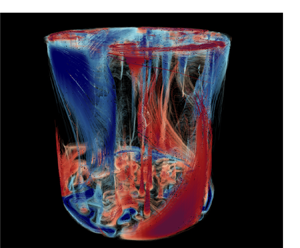
This transition also diminishes the difference between the bulk and the boundary flow in flow morphology. We show the streamlines for four cases in figure 6, where (a,b) corresponds to the coherent boundary flow state, and (c,d) the vortical boundary flow state. Comparing figures 6(a) and 6(b), one can see that the boundary flow structure for  $Ra=8.71\times 10^8$ is not much different from that for $Ra=8\times 10^7$, even though in the former case bulk convection has already emerged and the latter is below the onset of bulk convection. In figure 6(b) both the coherent boundary flow and bulk convective Taylor columns coexist. These two structures can be easily distinguished from the streamlines. For $Ra=1.02\times 10^9$, the system enters the vortical boundary flow state. As shown in figures 6(c) and 6(d), the boundary flow breaks into columns. In this case, it is difficult to distinguish the bulk and the boundary flows according to flow morphology. However, we remark that even in the vortical boundary flow state, the boundary flow and the bulk flow are still statistically different regions.

Figure 6. Streamlines coloured by the temperature fluctuation  $\theta -\langle \theta \rangle _{r,\phi }$ for (a) $Ra=8.0\times 10^7$, (b) $8.71\times 10^8$ (case ‘Before’), (c) $1.02\times 10^9$ (case ‘After’) and (d) $1.30\times 10^9$. All panels are with $\varGamma =1$, $Ek=1.85\times 10^{-6}$ and $Fr=0$.
Such transition in flow morphology also help to understand the influence of centrifugal force to  $Nu_{BF}$. For the cases with centrifugal force (set II), one can neither observe a sudden drop nor the $\varGamma$ dependence in $Nu_{BF}$ in figure 4(a). To understand such phenomenon, we present the vertical snapshots of the temperature field along the azimuthal direction at $r/R=0.95$ (within the boundary flow) in figures 7. In figures 7(a) and 7(c) we respectively present the temperature snapshots for the cases ‘Before’ and ‘After’ the transition, clearly depicting the change from the coherent boundary flow state to the vortical one. In figure 7(b) we present the snapshot of the case with parameters similar to the case ‘Before’ ( $Ra=8.71\times 10^8, \varGamma =1$), except that it has non-zero centrifugal force $Fr=0.12$. The temperature distribution in figure 7(b) exhibits noticeable differences from figure 7(a) (corresponding to case ‘Before’), but looks very similar to figure 7(c) (corresponding to case ‘After’). Instead of a coherent boundary flow structure, vortical columns are observed in figure 7(b), suggesting that the centrifugal force helps trigger the breakdown of the boundary flow. We also present the temperature field for $Fr=0.12$ and $Ra=1.02\times 10^9$ in figure 7(d), which has a similar $Ra$ to case ‘After’. Similar vortical flow structures can be observed in both figures 7(b) and 7(d), suggesting that the presence of the centrifugal force strongly suppresses the transition in boundary flow morphology. The breakdown of boundary flow coherency induced by the centrifugal force may then lead to a decrease in heat transport efficiency, as shown in figure 4. This could be the reason why no significant drop in $Nu_{BF}$ can be found for the cases with non-zero $Fr$, and their magnitudes of $Nu_{BF}$ are overall smaller than those with zero $Fr$.
$Fr$.

Figure 7. Vertical snapshots of the temperature field along the azimuthal direction at  $r/R=0.95$. The left panels refer to cases with $Fr=0$ and the right panels with $Fr=0.12$. The Rayleigh number for (a,b) is $Ra=8.71\times 10^8$ and for (c,d) is $1.02\times 10^9$. The aspect ratio $\varGamma$ equals to 1 for all cases. Snapshots (a,c) correspond to the cases ‘Before’ and ‘After’, respectively.
Additionally, we also observe a weak  $\varGamma$ dependence in the Reynolds number ( $Re$) of the boundary flow before the breakdown of boundary flow coherency. A drop in $Re$ can be found when the transition occurs, although the drop in $Re$ in much less significant than that of $Nu_{BF}$. Details of the Reynolds number for the boundary flow can be found in Appendix E.
3.4. Global heat transport in a cylindrical convection cell
With quantitative understandings of the heat transport in the bulk and the boundary flow, as respectively discussed in §§ 3.1 and 3.2, we are now in a position to explain the global Nusselt number. In this study we have two variables to indicate the flow state:  $Ra/Ra_w$ for the properties of the boundary flow and $Ra/Ra_c$ for the bulk. When we discuss the global heat transport, we first need to choose which variable would be a better choice. If we focus on the parameter range in which only geostrophic convection is present, the boundary flow always persists owing to the fact that $Ra_w$ is smaller than $Ra_c$. On the other hand, the bulk region can be either conductive or convective in this parameter range, depending on whether it is beyond the onset of bulk convection. In these two different bulk states, the heat transport of the bulk and, hence, the global one can be significantly different. To better distinguish conductive and convective bulk states, it will be convenient to use $Ra/Ra_c$ as the variable of choice for examining the global heat transport efficiency. Additionally, as discussed in 3.1, the scaling exponent $\gamma$ for $Nu_{bulk}\sim (Ra/Ra_c)^\gamma$ and $\gamma ^*$ for $Nu_{bulk}-1\sim (Ra/Ra_c-1)^{\gamma ^*}$ are in fact different when $Ra$ is close to onset of bulk convection. Such a difference may introduce inaccuracy when reconstructing the global $Nu$. Nevertheless, for $Ra/Ra_c\approx 1$, the contributions from the boundary flow are significant and the difference between the descriptions of $Nu_{bulk}$ may have a minor influence. For reason of simplicity, we hereby use $Nu_{bulk}\sim (Ra/Ra_c)^\gamma$ to describe the heat transport efficiency for the bulk. As for the boundary flow, (3.9) only captures the leading-order effect and (3.10) obviously provides a more precise description. Also for the purpose of a concise final result that could capture the dominating heat transport properties of the system, we use (3.9) for $Nu_{BF}$ in the following discussion. We also wish to remark that one can obtain a more precise description if more accurate (but probably more complicated) relationships for the $Nu_{bulk}$ and $Nu_{BF}$ are applied.
The global Nusselt number can be viewed as a superposition of the contributions from the bulk and the boundary flow. When the width of the boundary flow  $\delta _{BF}$ is much smaller than the cell radius $R$, we can assume that $r_{BF}/R\approx 1$. In this case, $Nu$ can be written as
 \begin{equation} Nu=\frac{r_{BF}^2}{R^2}Nu_{bulk}+\frac{R^2-r_{BF}^2}{R^2}Nu_{BF}\approx Nu_{bulk}+\frac{4\delta_{BF}/H}{\varGamma}Nu_{BF}. \end{equation}
For fixed  $Ek$ and $Ra\gtrsim Ra_c$, the heat transport efficiency of the boundary flow follows the power-law relation $Nu_{BF}\sim (Ra/Ra_w)^1$. We define $Nu_{BF}^c\equiv Nu_{BF}|_{Ra/Ra_c=1}$. We note that $Ek$ is fixed for sets I and II; thus, the local Nusselt number of the boundary flow can be written as
 \begin{equation} Nu_{BF}=Nu_{BF}^c (Ra/Ra_c)^1. \end{equation}
On the other hand,  $Nu_{bulk}$ can be described by the steep scaling $Nu_{bulk}\approx Ra/Ra_c^\gamma$. Thus, (3.11) is written as
 \begin{equation} Nu\approx (Ra/Ra_c)^\gamma+B (Ra/Ra_c)^1\ (Ra\gtrsim Ra_c), \end{equation}
where the prefactor  $B$ is defined as
 \begin{equation} B\equiv\frac{4\delta_{BF}/H}{\varGamma}Nu_{BF}^c. \end{equation}
For the coherent boundary flow state ( $Ra\leqslant Ra_t$), when the data obey (3.9), the width of boundary flow $\delta _{BF}$ is independent of $Ra$. Thus, for a given $\varGamma$ and $Ek$, the prefactor $B$ is roughly a constant. At $Ra=Ra_c$, one can obtain $B\approx Nu|_{Ra/Ra_c=1}-1$, wherein $B$ can be determined using $Nu$ at $Ra=Ra_c$. However, the existence of sidewall may slightly alter the onset of bulk flow, as shown in figure 3(a). Thus, the exact onset Rayleigh number of the bulk may need to be determined in experiments. We note that, for $Ra\lesssim Ra_c$, the $Ra$ dependence of $Nu$ is given by
 \begin{equation} Nu\approx1+B(Ra/Ra_c)^1\ (Ra\lesssim Ra_c), \end{equation}
which is noticeably different from (3.13). Thus, the exact onset Rayleigh number of the bulk convection and  $Nu|_{Ra=Ra_c}$ can be determined according to transition from (3.15) to (3.13). We plot $Nu$ vs $Ra$ in figure 8, and also (3.13) for $Ra>Ra_c^*$ and (3.15) for $Ra< Ra_c^*$ as dashed curves in the same figure. Here $Ra_c^*$ is the onset Rayleigh number determined according to the transition from (3.15) to (3.13). We remark that (3.15) is valid only when $Nu_{BF}$ follows (3.9). Due to the existence of the transitional regime, the Rayleigh number that (3.9) becomes valid is close to $Ra_c$ for sets I and II, as shown in figure 4(a). Thus, not all data for $Ra< Ra_c$ obey (3.15). Nevertheless, for cases beyond and below the onset of bulk convection, their $Ra$ dependences of $Nu$ are significantly different, so that $Nu|_{Ra=Ra_c}$ can still be determined. From figure 8, one can see that (3.13) can properly describe the obtained $Nu$ in the geostrophic regime. The red vertical dotted line corresponds to the transition in flow morphology in the boundary flow ( $Ra=Ra_t$). When the transition occurs, the scaling relation for the boundary flow (3.9) becomes invalid and $Nu$ gradually deviates from (3.13). As $Ra$ further increases, buoyancy gradually becomes dominant and $Nu$ asymptotically approaches the results of a non-rotating RBC.

Figure 8. Plot of  $Nu$ as a function of $Ra$ for sets I and II. The grey upper triangles are data collected from Funfschilling et al. (Reference Funfschilling, Brown, Nikolaenko and Ahlers2005). The dashed curves refer to (3.13) for $Ra>Ra_c^*$ and (3.15) for $Ra< Ra_c^*$. The red dotted line corresponds to $Ra=Ra_t$.
4. Conclusion
In this study we use a DNS approach to investigate the geostrophic rotating RBC in cylindrical cells. We explore the rotating RBC system in cylindrical cells with different aspect ratios and over a wide range of  $Ra$ from the onset of boundary flow to the rotation-unaffected regime. Our simulation yielded three data sets. Set I has $Ek$ fixed and $Ra$ varying and in set III we have $Ra$ fixed and $Ek$ varying. We compare these two data sets in order to reveal the $Ra$ and $Ek$ dependences of the heat transport and flow morphology of this system. As centrifugal force is inevitable in experiments, to ensure that our findings can be applied to the practical situations, set II is produced to study the effects of the centrifugal force. To understand the heat transport of this system with lateral boundaries, we decompose the bulk and the boundary flow and investigate these two domains separately.
We first focus on sets I and II with  $Ek$ fixed. For the bulk region, the $Ra$ dependence of $Nu_{bulk}$ is consistent with the numerical simulations using periodic boundary conditions. As for the boundary flow, after an intermediate regime, we observed a similar scaling relationship close to $Nu_{BF}\sim (Ra/Ra_w)^1$ for all cases. For set I, such a scaling relationship can be observed at $Ra/Ra_w\gtrsim 10$ ( $Ra\gtrsim \times 10^8$), and deviates from it at $Ra/Ra_w\approx 60$ ( $Ra\approx 1\times 10^9$). For set II, data for $Ra/Ra_w\lesssim 60$ ( $Ra\lesssim 1\times 10^9$) obey the above scaling relationship. By introducing the idea of boundary layer marginal stability theory, one can obtain the leading-order scaling relationship $Nu_{BF}\sim (Ra/Ra_w)^1$ if only the dominating term for $Ra_w$ is used, and a more precise description of the data can be obtained if the higher-order term in $Ra_w$ is considered.
As  $Ra$ increases, we observe a sharp transition in boundary flow morphology from the coherent state to the vortical state, which is accompanied by a sudden drop in $Nu_{BF}$. When the transition occurs, the scaling relationship $Nu_{BF}\sim (Ra/Ra_w)^1$ breaks down. The transitional Rayleigh number $Ra_t$ for $Ek=1.85\times 10^{-6}$ is found approximately equaling $8.71\times 10^8$ in our study. After the transition, the boundary flow breaks into vortices, manifesting the breakdown of flow coherency. Consequently, a drop in $Nu_{BF}$ can be observed as a result of the transition in flow morphology that the boundary flow becomes fragmented and heat exchange with the surrounding becomes more significant. After the transition, it becomes difficult to identify the bulk and the boundary flows based on flow morphology alone. Although this transition is difficult to discern from the global $Nu$, we remark that such a transition is well defined according to the sharp change in both $Nu_{BF}$ and the flow morphology. Additionally, comparing the temperature field for sets I and II, we find that the centrifugal force helps trigger the breakdown of the boundary flow and results in a weaker flow coherency. This probably is the reason why one cannot observe such a transition for the cases with non-zero $Fr$, and why $Nu_{BF}$ for the cases with zero $Fr$ is larger than those with non-zero ones. However, the current study is not sufficient to fully understand the influence of centrifugal force on the boundary flow. This would be an interesting topic for future studies.
Finally, we then revisit the global  $Nu$ and try to provide a unifying understanding. For the geostrophic rotating RBC, the global $Nu$ can be described by (3.13). When centrifugal force exists but does not significantly alter flow structures, its influence is reflected on the magnitude of the prefactor $B$ only and will not affect the scaling exponent. We further show that the prefactor $B$ can be determined using the global $Nu$. Thus, (3.13) can still be used to describe $Nu$ for experiments whether or not the centrifugal force is present. For set III with fixed $Ra$ and $Ek$ varying, the main discoveries are analogous to those for sets I and II, but with some variations in the width of the boundary flow and also the global $Nu$. Details of the discussions can be found in Appendix F.
Supplementary material
Supplementary material is available at https://doi.org/10.1017/jfm.2023.872.
Acknowledgements
We thank Professor J.-Q. Zhong for fruitful discussions. We also wish to thank an anonymous reviewer for suggesting the inclusion of higher-order correction in the marginal instability theory of the boundary layer.
Funding
This work is supported by the National Natural Science Foundation of China (grant no. 12072144, and 12232010); and the Research Grants Council of HKSAR (grant no. N_CUHK437/15).
Declaration of interests
The authors report no conflict of interest.
Appendix A. Validation of the decomposition method
We provide more examples for demonstrating the reliability of our method decomposing the boundary flow and the bulk. In figure 9 we provide the r.m.s. of the azimuthal velocity  $\langle u^2_\phi \rangle ^{1/2}_{t,z,\phi }$ and the convective heat flux $\langle J_z\rangle _{t,z,\phi }$ for $Ra=4.00\times 10^7$ and $1.30\times 10^9$, which respectively correspond to the case without bulk convection (wall mode only) and the vortical state that the boundary flow breaks into vortices. The results shown in figure 9 demonstrate that the two-layer boundary flow structure commences from the wall-mode state (figure 9a,c) and persists well into the turbulent state (figure 9b,d) in a rotating RBC system. Moreover, our method of decomposing the bulk and boundary flows works reliably for all these different states.

Figure 9. (a,c) The vertically averaged r.m.s. of azimuthal velocity  $\langle u^2_\phi \rangle ^{1/2}_{t,z,\phi }$, and (b,d) the convective vertical heat flux averaged temporally and in the vertical and azimuthal directions $\langle J_z\rangle _{t,z,\phi }$. All results are for the case of $Ek=1.85\times 10^{-6}$, $Fr=0$ and $\varGamma =1$. The Rayleigh number $Ra$ for (a,b) is $4.00\times 10^7$ and for (c,d) is $1.30\times 10^9$. The black dot-dashed and grey dashed lines respectively correspond to $r_{BF}$ and $r_0$. The grey dotted lines correspond to the linear fitting to the bulk part. The blue and red shaded regions respectively refer to the bulk and boundary flow. Insets correspond to the data for $r/R\in [0,1]$.
Appendix B. Details of the  $Nu_{BF}$ scaling relationship

As assumed in (3.7), the scaling relationship (3.9) requires that  $\varDelta _\delta /\varDelta$ being constant and that the thermal boundary layer dominating the heat transport. We examine the mean vertical temperature profiles of the boundary flow $\langle \theta \rangle _{t,r>r_{BF},\phi }$ for different $\varGamma$ in data set I ( $Fr=0$), as shown in figures 10(a)–10(c). According to whether $Nu_{BF}$ obeys the scaling relationship (3.9), we respectively plot the temperature profiles using solid (obey) and dot-dashed (not obey) curves. For small $Ra/Ra_w$, a large temperature gradient at the central region can be observed. As $Ra/Ra_w$ increases, the central temperature gradient decreases, leading to an increase in the temperature drop across the thermal boundary layer $\varDelta _\delta /\varDelta$, as illustrated by the black arrow in figure 10(a) for example. To quantitatively examine the approximation (3.7), we respectively fit the centre and boundary parts of the temperature profiles in figures 10(a)–10(c) using linear functions, and obtain $\varDelta _\delta /\varDelta$ and $\delta /H$ according to the intersection of these two linear fittings, as demonstrated by the inset of figure 10(a). The results of $\varDelta _\delta /\varDelta$ are presented in figure 10(d). The magnitude of $\varDelta _\delta /\varDelta$ increases as $Ra/Ra_w$ increases for $Ra/Ra_w\lesssim 10$, suggesting that the approximation (3.7) is not valid. This result explains why $Nu_{BF}$ for $Ra/Ra_w\lesssim 10$ does not obey the scaling relationship (3.9). On the other hand, broadly speaking, a saturation can be found in $\varDelta _\delta /\varDelta$ for $Ra/Ra_w\gtrsim 10$, and a small temperature gradient outside the boundary layer can be observed from figure 10(a–c) for the cases obeying (3.9). Approximation (3.7) requires that $\varDelta _\delta /\varDelta$ is insensitive to $Ra$, but it is not necessarily to be $1/2$. Thus, although $\varDelta _\delta /\varDelta$ exhibit $\varGamma$ dependence when it reaches a plateau, it does not affect the derivation of the scaling relationship. These results help validate the approximations for (3.9) and explain why, for $Ra/Ra_w\lesssim 10$, the data do not obey (3.9).

Figure 10. Temperature distribution  $\langle \theta \rangle _{t,r>r_{BF},\phi }$ averaged horizontally and temporally in the boundary flow for (a) $\varGamma =0.5,\ Fr=0$, (b) $\varGamma =1,\ Fr=0$ and (c) $\varGamma =2,\ Fr=0$ (all data from set I). The solid (dot-dashed) curves refer to the cases obeying (not obeying) the scaling relationship $Nu_{BF}\sim (Ra/Ra_w)^1$. The inset of (a) illustrates the definitions of $\delta /H$ and $\varDelta _\delta /\varDelta$. The dashed lines in the inset denote the linear fittings of the centre and boundary profiles. (d) The normalized temperature drop $\varDelta _\delta /\varDelta$ as a function of $Ra/Ra_w$.
Additionally, in § 3.2 we provide a higher-order correction for the  $Ra$ dependence of $Nu_{BF}$. Here we provide a detailed derivation of (3.10). By using the full terms of $Ra_w$ given by (1.2), then the marginal instability argument of the thermal boundary layer $Ra_w^\delta \sim Ra^\delta$ can be written as
 \begin{equation} {\rm \pi}^2\sqrt{6\sqrt{3}}\frac{1}{Ek^\delta}+\frac{46.55}{(Ek^\delta)^{2/3}}\sim\frac{\alpha g\varDelta^\delta\delta^3}{\kappa\nu}. \end{equation}
Assuming  $\varDelta ^\delta /\varDelta \approx 0.5$ and $Nu\approx (\varDelta ^\delta /\delta )/(\varDelta /H)$, one can then obtain
 \begin{equation} Nu_{BF}\bigg({\rm \pi}^2\sqrt{6\sqrt{3}}+46.55Ek^{1/3}\left(\frac{\varDelta}{\varDelta^\delta}Nu_{BF}\right)^{2/3}\bigg)\sim RaEk, \end{equation}
which is the equation given by (3.10) and it is obviously not a power-law relationship. To determine the solution of (3.10), one needs to introduce additional constrains, i.e.
 \begin{equation} Nu_{BF}\bigg({\rm \pi}^2\sqrt{6\sqrt{3}}+46.55Ek^{1/3}\left(\frac{\varDelta} {\varDelta^\delta}Nu_{BF}\right)^{2/3}\bigg)\approx ARaEk, \end{equation}
where  $A$ is the fitting parameter so that the solution of (B3) matches the magnitudes of the numerical data. The grey curves shown in figure 4(a) are the solutions solved in the above way.
Appendix C. Influence of the mode number of the boundary flow
The  $\varGamma$ dependence of the parameter $C$ shown in table 1 reveals the fact that local heat transport efficiency in the boundary depends on the aspect ratio. Such dependence on the aspect ratio is surprising, as other quantities such as $Nu_{bulk}$ and $\delta _{BF}$ exhibit no significant $\varGamma$ dependence, and $Nu_{BF}$ for different $\varGamma$ originally collapse together when $Ra/Ra_w$ is close to unity but start to diverge as $Ra$ increases. As we discuss in § 3.3, the fragmentation of the coherent boundary flow could lead to a drop of $Nu_{BF}$, which suggests the connection between the typical length scale of the boundary flow and the local heat transport efficiency. We note that the mode number $N$ of the boundary flow is always an integer, and the unit sizes of the boundary flow ( $2{\rm \pi} R/N$) are different among different aspect ratios. Thus, a possible reason for the $\varGamma$ dependence of $Nu_{BF}$ may be attributed to the difference in unit sizes of the boundary flow between different aspect ratios.
To examine the connection between the unit size  $2{\rm \pi} R/N$ of the boundary flow and $Nu_{BF}$, we provide a set of data with the same aspect ratio 1 ( $R$ is fixed) but a different mode number $N$. Comparing the results with different $N$ but similar $R$ or $\varGamma$ may help eliminate the possible influence related to the aspect ratio. We find that by using an initial flow field whose boundary flow has a specific mode number $N$, the boundary flow can be locked in the chosen mode number $N$ when the system is stable. The boundary flow for $\varGamma =1$, $Fr=0$ discussed previously and for most cases in the rest of this study has mode number $N=3$. By using the initial field with $N=2$, we can control the mode number of the stable state. We present an example for $Ra=3.4\times 10^8$ and $\varGamma =1$ in figures 11(a) and 11(b), demonstrating that the azimuthal mode number can be selected to be either $N=2$ (figure 11a) or $N=3$ (figure 11b). Since $\lambda ={\rm \pi} \varGamma /N$ is inversely proportional to $N$, the cases with $N=2$ have larger $\lambda$ than those with $N=3$. Using this method, we can control the mode number $N$ and the wavelength $\lambda$ without changing the aspect ratio. We remark that only cases for $Ra\leqslant 5.12\times 10^8\ (Ra/Ra_w\lesssim 30)$ can have a stable mode number of $N=2$ for $\varGamma =1$. We speculate that, for high $Ra$, the system is more turbulent, which could make the boundary flow less coherent and more difficult to be stabilized in a state with a small mode number. The change of preferred mode number as $Ra$ increases was also observed in a previous study (Zhong et al. Reference Zhong, Ecke and Steinberg1993).

Figure 11. (a,b) Snapshots of the temperature distributions at the mid-height for the modes  $N=2$ and $N=3$ (both in $\varGamma =1$ cell), respectively. The Rayleigh number for these two cases is $3.40\times 10^8$, and the Froude number is zero. The grey dashed and black dot-dashed circles respectively correspond to $r=r_0$ and $r=r_{BF}$. Plot of (c) $Nu_{BF}$ and (d) $Nu$ for both $N=2$ and $N=3$ (legends are the same as in c). Both these cases are for $\varGamma =1$ and $Fr=0$.
From figure 11(c) we see that  $Nu_{BF}$ for the internal mode $N=2$ are overall larger than for the internal mode $N=3$, demonstrating that the heat transport efficiency is positively related to unit size (inversely proportional to the mode number $N$) within the boundary flow. The mode number dependence of heat transport efficiency is not a minor effect that is not only reflected on $Nu_{BF}$, but it also has significant influence on the global Nusselt number. We compare $Nu$ for $N=2$ and $N=3$ in figure 11(d) and find that $Nu$ for $N=2$ is noticeably larger than that of $N=3$, albeit the two modes (flow states) are nominally under an identical set of global control parameters and boundary conditions, indicating the existence of multiple states in the boundary flow. We remark that the multiple state can be observed up to $Ra/Ra_w\approx 30$, which is well beyond the onset of the boundary flow. Additionally, both $Nu$ and $Nu_{BF}$ exhibit significant dependence on the mode number. On the contrary, in the wall-mode state the heat transport efficiency is not very sensitive to the mode number (Zhong et al. Reference Zhong, Ecke and Steinberg1993), which can also be seen from figures 11(c) and 11(e) that $Nu_{BF}$ and $Nu$ for the lowest $Ra$ of $N=2$ have roughly similar values with those of $N=3$. For the reasons we mentioned above, we infer that the multiple states observed in this study are different from the linear mode with an integer mode number in the azimuthal direction when the boundary flow (or wall mode) first emerges. To the best of our knowledge, this is also the first time reporting the influence of multiple states to the heat transport in the boundary flow well beyond the onset. Since the global Nusselt number is sensitive to the mode number, it is crucial to track the mode number when conducting global Nusselt measurements. On the other hand, it is interesting and also important to systematically investigate mode evolution of the boundary flow in long-term experiments and also the mechanism inducing the mode number dependence of local heat transport efficiency in future studies.
Appendix D. Distribution of vortex density
The distribution of temperature fluctuation  $\theta _{rms}\equiv (\langle \theta ^2\rangle _{t}-\langle \theta \rangle ^2_{t})^{1/2}$ reflects the evolution of the flow structures in the system. Figure 12 presents the temperature fluctuations averaged over the azimuthal direction $\langle \theta _{rms}\rangle _{\phi }$ for different $Ra$. For $Ra$ close to the onset of the wall mode shown in figure 12(a), the temperature fluctuations are mainly found within the boundary flow (wall mode in this state). Since the $Ra$ for figure 12(a) is below the onset of bulk convection, $\theta _{rms}$ is negligible for the majority of the bulk, especially for the regions near the top and bottom plates. When $Ra$ is beyond the onset of bulk convection, as shown in figure 12(b) with $Ra\approx Ra_c$, the regions near the top and bottom plates show strong temperature fluctuations, which may be attributed to the thermal boundary layers. As for the boundary flow, temperature fluctuations are maximized within the outer boundary flow (with positive azimuthal velocity). A similar distribution of $\theta _{rms}$ can be found in figure 12(c), corresponding to the case ‘Before’ in the coherent boundary flow state. One may note that regions with high temperature fluctuation may exceed the boundary flow (vertical black dot-dashed lines) for figures 12(a)–12(c). Such distribution corresponds to the emission of the plume-like structures as discussed in § 3.3 and shown in figure 5(a). Due to the weak convective mixing in this state, the plume-like structures are able to preserve the heat contents after radial emission. When the transition in flow morphology occurs and the boundary flow breaks into vortical columns, one can observe a vertically expanded region with strong temperature fluctuations roughly centralized at $r_0$. In this case, the bulk convection is sufficiently strong to mix the flow structures emitting from the boundary flow, so that one cannot observe high temperature fluctuations in the bulk. As $Ra$ further increases, temperature fluctuations are strongest at the area adjacent to the top and bottom plates, as shown in figure 12(e). Focusing on the radial distribution, one can still observe a vertically expanded region maximizing at $r_0$, corresponding to the columnar structures.

Figure 12. Temperature fluctuation  $\langle \theta _{rms}\rangle _{\phi }$ averaged over the azimuthal direction for (a) $Ra=2.00\times 10^7$, (b) $3.40\times 10^8$, (c) $8.71\times 10^8$ (case ‘Before’), (d) $1.02\times 10^9$ (case ‘After’) and (e) $1.54\times 10^9$. All panels are with $\varGamma =1$ and $Fr=0$. The lower row refers to the radial distributions of vortex density for ( f) $Ra=8.71\times 10^8$, (g) $1.02\times 10^9$ and (h) $3.07\times 10^9$. All vertical grey dot-dashed and dashed lines respectively correspond to $r_{BF}$ and $r_0$, and the red inclined dashed lines in ( f–h) refer to the uniform distribution $P_\omega (r)=2r/R^2$.
The distribution of the vortex is discussed. We extract the vortices using the  $Q$ criterion (Hunt, Wray & Moin Reference Hunt, Wray and Moin1988). The method of vortex extraction we used in this study is similar to those in Chong et al. (Reference Chong, Shi, Ding, Ding, Lu, Zhong and Xia2020) and Ding et al. (Reference Ding, Chong, Shi, Ding, Lu, Xia and Zhong2021). The vortex density distribution function $P_\omega$ for different Rayleigh numbers are shown in figures 12( f)–12(h), wherein ( f) corresponds to the coherent boundary flow state ( $Ra=8.71\times 10^8$) and (g,h) the vortical boundary flow state ( $Ra=1.02\times 10^9$ and $3.07\times 10^9$). For comparison, we also show the density for uniform distribution $P_\omega (r)=2r/R^2$. We find that for the coherent boundary flow state, $P_\omega$ peaks at $r=r_0$, suggesting that most columnar vortices in the system originate from the boundary flow. Although more columnar vortices are emerging from the bulk, the maximum of $P_\omega$ is still at $r=r_0$, meaning that the boundary flow generates columnar vortices more frequently than the bulk. Comparing figures 12( f)–12(h), we find that the vortex density gradually approaches a uniform distribution as $Ra$ increases, but the boundary still has a higher vortex density even at $Ra=3.07\times 10^9$ ( $Ra/Ra_c\approx 9.1$, corresponding to the vortical boundary flow state).
Appendix E. Reynolds number of the bulk and the boundary flow
Other than the heat transport, the flow strength of the boundary flow is also an important quantity depicting the evolution of the system. The flow strength of the boundary flow is represented by the Reynolds number
 \begin{equation} Re\equiv u\sqrt{Ra/Pr}. \end{equation}
As we discuss in § 2.2, the mean velocity of the boundary flow cannot correctly reflect its flow strength due to the periodicity. For this reason, we use the r.m.s. of different velocity components to evaluate the Reynolds number. In this study we define six different Reynolds number, as shown in figure 13. The subscripts in  $Re_{*,BF}$ and $Re_{*,+}$ respectively denote the Reynolds numbers evaluated using the mean velocity r.m.s. of the boundary flow $\langle u_*^2 \rangle ^{1/2}_{t,z,\phi,r\geqslant r_{BF}}$ and the outer boundary flow $\langle u_*^2 \rangle ^{1/2}_{t,z,\phi,r\geqslant r_{0}}$, and $Re_{*,bulk}$ refers to the average over the bulk, i.e. $\langle u_*^2 \rangle ^{1/2}_{t,z,\phi,r\leqslant r_{BF}}$. The subscripts in $Re_{\phi,*}$ and $Re_{z,*}$ respectively represent the Reynolds number for the azimuthal $u_\phi$ and vertical components $u_z$. As shown in figure 13, we find that all four Reynolds numbers follow a scaling relationship $Re\sim (Ra/Ra_w)^1$. We remark that in the experiments conducted by Wedi et al. (Reference Wedi, Moturi, Funfschilling and Weiss2022) they found that the maximum velocity normalized by the free-fall velocity $u^{max}_\phi$ follows a scaling relationship $u^{max}_\phi =4.7 Ek^{3/2}Ra^{1/2} Pr^{0.8}$. According to our definitions of the Reynolds number (E1), their results also suggest a scaling relationship $Re\sim (Ra/Ra_w)^1$ as we observed in figure 13, although they use the maximum instead of the mean velocity and their parameters are far beyond the bulk onset $Ra_c$, meaning that their experiments should mainly belong to the vortical boundary state. Additionally, from figure 13 we can also observe a drop in $Re$ when the transition of flow morphology occurs, although the drop in $Re$ is less significant than that of $Nu_{BF}$. As for the bulk flow shown in figures 13(e) and 13( f), one can observe non-zero flow strength below the onset of the bulk flow, which is induced by the shearing of the boundary flow. In this state one can observe a $\varGamma$ dependence in both $Re_{\phi,bulk}$ and $Re_{z,bulk}$, which should arise from the different bulk averaging areas. As the bulk convection emerges, both $Re_{\phi,bulk}$ and $Re_{z,bulk}$ become more sensitive to $Ra$ and gradually become comparable with the flow strength of the boundary flow. Additionally, the data for all cases collapse together, which is similar to those observed in $Nu_{bulk}$, as shown in figure 3.

Figure 13. Plots of (a,b)  $Re_{*,BF}$, (c,d) $Re_{*,+}$ and (e, f) $Re_{*,bulk}$ for the cases in sets I and II. The grey dot-dashed lines represent $Re\sim (Ra/Ra_w)^1$. The vertical dotted lines correspond to $Ra=Ra_t$, and the grey vertical dashed lines refers to $Ra=Ra_c$.
Appendix F. Results for the cases with fixed $Ra$

In this system the heat transport efficiency of the bulk is usually considered as a function of  $Ra/Ra_c$, while for the boundary flow, $Nu_{BF}$ is a function of $Ra/Ra_w$. In the previous sections we focused on the cases with $Ek$ fixed and $Ra$ varying, wherein $Ra/Ra_c$ and $Ra/Ra_w$ only differ by a constant, thus it would be easy to unify the different scaling relationships for the bulk and the boundary flow. However, since $Ra_c$ and $Ra_w$ have different $Ek$ dependence, when $Ra$ is fixed and $Ek$ varying, extra efforts may be required to unify the heat transport efficiency of different regions. Moreover, some responding parameters (such as the thickness of the boundary flow) may have significant $Ek$ dependence that could affect the global heat transport. Thus, it is important to examine our findings in the cases where $Ek$ is changed. In this section we concentrate on the data from set III, which has $Ra$ fixed and $Ek$ varying. The heat transport of the bulk and the boundary flows for set III will be discussed.
We first examine the width of the boundary flow for set III. Using a similar method as described in § 2.2, we obtain  $\delta _{BF}$ and $\delta _{0}$ for set III. We present the results as functions of $Ek$ in figure 14. Different from sets I and II wherein $\delta _{BF}$ and $\delta _{0}$ are largely not sensitive to $Ra$, one can observe clear $Ek$ dependence in figure 14. According to the $Ek$ dependence of $\delta _{BF}$ and $\delta _{0}$, we respectively fit the data for $Ek\leq 3.67\times 10^{-5}$ and $Ek\geq 3.67\times 10^{-5}$ using $\delta \sim Ek^\beta$, where $\beta$ is the exponent of the power law, and present the best fit results in figure 14. For small $Ek$ ( $Ek\leq 3.67\times 10^{-5}$), we obtain $\delta _0\sim Ek^{0.38}$, which is close to the thickness of the outer Stewartson layer (the portion close to the sidewall) $Ek^{1/3}$ (Kunnen, Clercx & Van Heijst Reference Kunnen, Clercx and Van Heijst2013). As for $\delta _{BF}$, we observe a scaling relationship $\delta _{BF}\sim Ek^{0.21}$ for $Ek\leq 3.67\times 10^{-5}$, which is also close to the thickness of the inner Stewartson layer (the portion away from the sidewall) $Ek^{1/4}$. For large $Ek$ ( $Ek\geq 3.67\times 10^{-5}$), we find that $\delta _{0}$ follows $\delta _0\sim Ek^{0.67}$. This result agrees with the scaling relationship $\delta _0\sim Ek^{2/3}$ suggested by Zhang et al. (Reference Zhang, Ecke and Shishkina2021). As for $\delta _{BF}$, we observe a slightly smaller exponent $\delta _{BF}\sim Ek^{0.57}$. We remark that such a scaling is close to the scaling relationship $\delta _0\sim Ek^{1/2}$ indicated by Wedi et al. (Reference Wedi, Moturi, Funfschilling and Weiss2022), although they were studying $\delta _0$ instead of $\delta _{BF}$ in their paper. The transitions from $\delta _0\sim Ek^{0.38}$ to $\delta _0\sim Ek^{0.67}$ and from $\delta _{BF}\sim Ek^{0.21}$ to $\delta _{BF}\sim Ek^{0.57}$ are consistent with the breakdown of coherent boundary flow into columnar vortices, as we discuss next.

Figure 14. Width of the boundary flow  $\delta _{BF}$ and outer boundary flow $\delta _{0}$ for set III ( $Ra$ fixed and $Ek$ varying). The open (solid) symbols refer to $\delta _{0}$ ( $\delta _{BF}$). The dashed and dot-dashed lines respectively refer to the best fits for the data with $Ek\leq 3.67\times 10^{-5}$ and $Ek\geq 3.67\times 10^{-5}$.
Analogous to §§ 3.1 and 3.2, we decompose the bulk and the boundary flow and examine the heat transport for these two regions separately for set III. We present the results for  $Nu_{bulk}$ for set III in figure 15(a). Similar to sets I and II with fixed $Ek$ shown in figure 3(a), $Nu_{bulk}$ equals 1 for $Ra/Ra_c<1$, meaning that heat transport in the bulk is through conduction before the onset of bulk convection. As for $Ra/Ra_c>1$, bulk convection emerges and $Nu_{bulk}$ increases as $Ra/Ra_c$ increases. Similar to the cases with periodic boundary conditions, one can also observe a steep scaling relationship $Nu_{bulk}\sim (Ra/Ra_c)^{3.3\pm 0.3}$ for set III. As $Ra/Ra_c$ further increases, the rotating rate and the strength of the Coriolis force decrease. Since we fix $Ra$ in set III, the magnitude of $Nu_{bulk}$ gradually approaches a constant corresponding to the non-rotating case.

Figure 15. Plots of (a)  $Nu_{bulk}$ and (b) $Nu_{BF}$ for set III ( $Ra$ fixed and $Ek$ varying). The cross symbols in (a) are data with lateral periodic boundary conditions for comparison, and the grey dashed line refers to $Nu_{bulk}\sim (Ra/Ra_c)^{3.3}$. The red dot-dashed line in (b) refers to $Nu_{BF}\sim (Ra/Ra_w)^1$. Plots (c,d) correspond to the power spectrum of the temperature distribution along the azimuthal direction at $r/R=1,\ z/H=0.5$, and (e, f) present the space–time plot of the temperature at the same location. Plots (c,e) and (d, f) respectively correspond to the case $Ra/Ra_w\approx 16$ and $20$ (i.e. before and after the transition), as indicated by the arrows in (b).
We now examine the results of  $Nu_{BF}$ for set III, as shown in figure 15(b). Similar to sets I and II, we can also observe some of the data following the scaling relationship (3.9). Comparing figures 15(a) and 15(b), we find that the three smallest data points for $Ra/Ra_w$ still obey (3.9), which are well below the onset Rayleigh number $Ra_c$ of bulk convection. This is quite different to the results of sets I and II shown in figure 4(a). In those cases, the Rayleigh number that $Nu_{BF}$ begins to be governed by (3.9) is close to $Ra_c$. This result also suggests that the Rayleigh number for (3.9) being valid does not necessarily equal $Ra_c$. The close magnitudes of these two Rayleigh numbers in figure 4(a) could probably be a coincidence. As $Ra/Ra_w$ further increases, $Nu_{BF}$ becomes less sensitive to $Ra/Ra_w$, although one cannot observe a sudden drop in $Nu_{BF}$ as can be found in set I ( $\varGamma =1$ and $2$,
$2$,  $Fr=0$, for example). This change of $Nu_{BF}$ behaviour is also attributed to the transition in flow morphology of the boundary flow. Since set III has $\varGamma =4$ and a relatively large mode number $N$, it may be difficult to identify the breakdown of the coherent boundary flow into columnar vortices from the temperature field. For this reason, we instead present the time-averaged power spectrum density $E_\theta$ of the temperature distribution along the azimuthal direction at $r/R=1$, $z/H=0.5$ in figure 15(c,d). For figure 15(c) with $Ra/Ra_w\approx 16$ (coherent boundary flow state), one can observe a clear peak in $E_\theta$, meaning that the boundary flow is coherent and with a strong azimuthally periodic pattern. As for figure 15(d) ( $Ra/Ra_w\approx 20$), one could still find a peak at the azimuthal frequency of 20, but its magnitude is much reduced compared with that of 15(c) ( $Ra/Ra_w\approx 16$), showing that the boundary flow is not coherent and breaks into vortices, i.e. the system enters the vortical boundary flow state. Such a transition in flow morphology can be better illustrated from the space–time plot of the sidewall temperature. Figure 15(e) (corresponding to the case before transition) depicts a coherent boundary flow state with band-like structures in the space–time plot. On the other hand, as can be seen from figure 15( f), one can see that the boundary flow becomes fragmented, suggesting the transition of the boundary flow morphology to a vortical state. The results shown in figures 15(b)–15( f) depict a similar physical picture as figures 4(a) and 5: when the coherent boundary flow breaks down into columnar vortices, the characteristic length scale of the boundary flow decreases. As a result, the boundary flow structure becomes less coherent and the heat transport efficiency drops. We define $Ek_t$ as the transitional Ekman number of the boundary flow when $Ra$ is fixed. According to the changes in flow morphology and $Nu_{BF}$, $Ek_t$ roughly equals $2.66\times 10^{-5}$ for $Ra=2\times 10^7$, corresponding to $Ra/Ra_w\approx 16$.
Another important finding of this study is the relationships (3.13) and (3.15) describing the global Nusselt number. When deriving (3.13) and (3.15), we assume that  $\delta _{BF}$ is insensitive to the change of $Ra$. However, as shown in figure 14, $\delta _{BF}$ has significant $Ek$ dependence. For this reason, we need to modify the derivation in § 3.4.
Starting from (3.11), we assume  $\delta _{BF}/H\sim Ek^{1/4}$ according to figure 14 and also the scaling relationship of the inner Stewartson layer. Using the relation (3.9), (3.11) can be written as
 \begin{equation} Nu\approx (Ra/Ra_c)^\gamma+B^\prime(Ra/Ra_c)Ek^{{-}1/12}\quad(Ra/Ra_c\geq1), \end{equation}
where  $B^\prime$ is the prefactor defined as
 \begin{equation} B^\prime\equiv \frac{4\delta_{BF}^c/H}{\varGamma}Nu_{BF}^c(Ek^c)^{1/12}. \end{equation}
Here  $\delta _{BF}^c$ is defined as $\delta _{BF}^c\equiv \delta _{BF}|_{Ra/Ra_c=1}$, and $Ek^c$ is the onset Ekman number of the bulk convection for the fixed $Ra$ ( $Ra=2\times 10^7$ for this data set). Similar to those discussed in § 3.4, such a prefactor $B^\prime$ can be determined according to just the Nusselt number at $Ra/Ra_c-1$,
 \begin{equation} B^\prime=[Nu|_{Ra/Ra_c=1}-1](Ek^c)^{1/12}. \end{equation}
As for  $Ra/Ra_c<1$, we let $Nu_{bulk}=1$ and one can obtain
 \begin{equation} Nu\approx 1+B^\prime(Ra/Ra_c)Ek^{{-}1/12}\quad(Ra/Ra_c\leq1). \end{equation}
Comparing (3.13) with (F1) and (3.15) with (F4), one sees that the main difference is the prefactor  $Ek^{-1/12}$. However, the exponent of this prefactor is so small that it is reasonable to neglect its variation, i.e. $Ek^{-1/12}\approx Ek_c^{-1/12}$. Then, (F1) is reduced to (3.13) and (F4) to (3.15). Thus, even though $\delta _{BF}$ has significant $Ek$ dependence, as shown in figure 14, $Nu$ can still be described by (3.13) and (3.15) at the leading order.
We present the data of  $Nu$ as a function of $Ra/Ra_c^*$ in figure 16. Here $Ra_c^*$ is the onset Rayleigh number determined according to the transition from (F4) to (F1). We also plot (F4) and (F1) as the dashed curve in figure 16. The grey dotted line in figure 16 corresponds to the transition in flow morphology, which is determined by the drop of $Nu_{BF}$ ( $Ek=2.66\times 10^{-5}$ and $Ra/Ra_c^*\approx 1.9$). One can see that (F4) and (F1) can properly describe the data before the transition occurs. Similar to sets I and II, for $Ra/Ra_c^*$ beyond the transition, (F1) begins to deviate from the data of $Nu$, which is attributed to the breakdown of (3.9). Since in set III $Ra$ is fixed, when $Ra/Ra_c^*$ further increases, $Nu$ gradually approaches a constant corresponding to the non-rotating case ( $Nu$ for the fixed $Ra$). Additionally, all $Nu$ for $Ra/Ra_c^*\leq 1$ consist with (F4). We remark that this could be attributed to the fact that the parameter range of $Ek$ does not extend to the onset of the wall mode. When $Ek$ further decreases ( $Ra/Ra_c^*$ decreases), we may also observe an intermediate regime not obeying (F4), which has been found in $Nu$ for set I (as shown in figure 8). This result also suggests that $Ra/Ra_c\approx 1$ is not a required condition for (3.9) to become valid. In other words, the onset of bulk convection could be independent of the heat transport of the boundary flow.


