


1. Introduction
The advent of superhydrophobic surfaces, originally designed to facilitate conditions for non-wetting drops (Quéré Reference Quéré2005, Reference Quéré2008), has led to a surge in interest of liquid flows about microstructured surfaces consisting of solid patches and air bubbles (Rothstein Reference Rothstein2010). The most common of these are periodic arrays of slats, with air bubbles trapped in the respective grooves (Ou & Rothstein Reference Ou and Rothstein2005; Tsai et al. Reference Tsai, Peters, Pirat, Wessling, Lammertink and Lohse2009), and doubly periodic pillar arrays, where air is trapped in the continuous region surrounding the pillars (Joseph et al. Reference Joseph, Cottin-Bizonne, Benoît, Ybert, Journet, Tabeling and Bocquet2006; Lee, Choi & Kim Reference Lee, Choi and Kim2008). Owing to the dominance of capillarity at small scales, the liquid–air menisci are of uniform curvature. In particular, the cylindrical bubbles trapped in the groove-array surface possess the cross-sectional shape of a circular arc.
The slipperiness of a compound surface is characterised by the slip length (Bocquet & Barrat Reference Bocquet and Barrat2007), the fictitious distance below the surface at which an imposed shear profile extrapolates to zero. For the non-isotropic groove-array geometry, two canonical shear problems emanate: the ‘longitudinal’ one, where the shear is applied parallel the grooves; and the ‘transverse’ one, where it is applied perpendicular to them. The ratio of the slip length to the period depends upon the parameters quantifying the surface geometry, and in particular the solid fraction  $\epsilon$, representing (on a single period) the ratio of the wetted-solid area to the total area.
In modelling the canonical problem governing the slip length, it is common to neglect the viscosity of the trapped air. Since a free surface cannot support a shear force, the problem is ill-posed for  $\epsilon =0$ and is consequently singular for $\epsilon \ll 1$, implying a divergent slip length. A first illustration of that singularity was provided by Philip (Reference Philip1972) for both the longitudinal and transverse problems in the simplest case of flat menisci, where the corresponding slip-length formulae diverge as $\ln \epsilon$ (Lauga & Stone Reference Lauga and Stone2003). Given the pragmatic desire to maximise slip lengths (Choi & Kim Reference Choi and Kim2006; Lee et al. Reference Lee, Choi and Kim2008), there is a fundamental interest in understanding the small-solid-fraction singularity. A scaling analysis by Ybert et al. (Reference Ybert, Barentin, Cottin-Bizonne, Joseph and Bocquet2007) suggested an algebraic slip-length singularity, as $\epsilon ^{-1/2}$, for the pillar-array configuration. For the groove-array configuration, no singularity was predicted; alluding to Philip (Reference Philip1972), Ybert et al. (Reference Ybert, Barentin, Cottin-Bizonne, Joseph and Bocquet2007) proposed a weak logarithmic singularity.
These scaling arguments were later tested against detailed analyses. While the  $\epsilon ^{-1/2}$ singularity was indeed confirmed for pillar arrays (Davis & Lauga Reference Davis and Lauga2010; Schnitzer & Yariv Reference Schnitzer and Yariv2018), the predicted logarithmic singularity for groove arrays turns out to be incompatible with longitudinal slip-length calculations in the special case of $90^{\circ }$ protrusion angles (Crowdy Reference Crowdy2015). In a pioneering asymptotic analysis, Schnitzer (Reference Schnitzer2016) showed that the singularity is in fact algebraic in that case, scaling as $\epsilon ^{-1/2}$. Following that work, it was observed that $90^{\circ }$ protrusion angles may lead to other peculiarities in longitudinal flows about groove arrays, such as an anomalous pressure-driven plug flow (Yariv & Schnitzer Reference Yariv and Schnitzer2018).
The above investigations of groove-array geometries have been carried out assuming that the menisci are pinned at the edges of the slats. Under large pressures, however, the liquid may partially invade the grooves (Lee & Kim Reference Lee and Kim2009; Lv et al. Reference Lv, Xue, Shi, Lin and Duan2014). Thus, rather than being pinned, the contact lines of the liquid–air menisci are displaced a finite distance into the grooves. When modelling partially invaded configurations, one may conveniently take the slats to be infinitely thin (Crowdy Reference Crowdy2021); the finite solid–liquid contact area on the sides of the slats, which vanishes in the ‘conventional’ non-invaded configuration, then effectively defines the solid fraction. For flat menisci, the longitudinal problem was solved in closed form by Crowdy (Reference Crowdy2021); consistently with the scaling arguments of Ybert et al. (Reference Ybert, Barentin, Cottin-Bizonne, Joseph and Bocquet2007), it exhibits a logarithmic singularity.
Crowdy (Reference Crowdy2021) also calculated the effect of small protrusion angles. As this results in a regular perturbation about the nominal flat-meniscus geometry, it also exhibits a logarithmic singularity. Presently, no analytic or numerical solution is known for finite protrusion angles. Inspired by the analysis of conventional surfaces (Schnitzer Reference Schnitzer2016), we here consider the partially invaded configuration in the extreme case of  $90^{\circ }$ protrusion angles, addressing the singular small-solid-fraction limit from the outset. Our goal is to illuminate the non-conventional singularity mechanism in that idealised configuration.
2. Problem formulation
The microstructure considered herein consists of a periodic array (period  $2a$) of slats, with air trapped in the enclosed grooves. The contact lines of the liquid–air menisci are displaced a finite distance $\epsilon a$ ( $\epsilon >0$) into the grooves. Following earlier analyses (Crowdy Reference Crowdy2021; Miyoshi et al. Reference Miyoshi, Rodriguez-Broadbent, Curran and Crowdy2022), we assume that the slats are infinitely thin; then, $\epsilon$ represents the solid fraction of the microstructure. The curved menisci adopt a cross-sectional shape of a circular arc; we consider here the idealised scenario of a $90^{\circ }$ protrusion angle, whereby
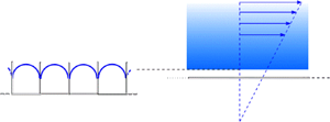
  $a$ coincides with the bubble radius. The periodic geometry is portrayed in figure 1(a).

Figure 1. (a) Dimensional problem for a  $90^{\circ }$ protrusion angle bubble mattress. (b) Dimensionless unit-cell problem governing the longitudinal velocity.
Following the canonical problem in the field (Davis & Lauga Reference Davis and Lauga2009), our interest is in the flow that is animated by an imposed shear (magnitude  $G$) at large distances. We are concerned here only with the longitudinal problem which arises when the shear flow is pointing along the grooves. The flow is then unidirectional (Crowdy Reference Crowdy2010), and the velocity is governed by a two-dimensional problem in the cross-sectional plane.
Normalising length variables by  $a$, we employ Cartesian coordinates $(x_1=x,\ x_2=y,\,x_3)$ with the $xy$ plane perpendicular to the flow, the $y$ axis passing through the contact lines (points in the cross-sectional plane), and the $x$ axis passing through one of these lines, pointing into the liquid. Owing to periodicity, it suffices to consider a single ‘unit cell’, say, that bounded between $y=\pm 1$. The associated two-dimensional liquid domain, say, $\mathcal {D}$, is bounded by (i) the periodicity rays,
 \begin{equation} \mathcal{P}{:} \quad y=\pm1, \quad x>1; \end{equation}
(ii) the menisci,
 \begin{equation} \mathcal{M}{:} \quad y={\pm} f(x), \quad 0< x<1, \end{equation}
where
 \begin{equation} f(x) = 1-\sqrt{1-x^2}; \end{equation}
and (iii) the solid slat,
 \begin{equation} \mathcal{S}{:} \quad 0< x<\epsilon, \quad y=0. \end{equation}
 The fluid velocity, normalised by  $Ga$, is $\hat {\boldsymbol {e}}_3 w$. The longitudinal component, $w(x,y;\epsilon )$, is governed by a unit-cell problem consisting of (i) Laplace's equation, $\nabla ^2w=0$ in $\mathcal {D}$; (ii) the periodicity conditions, $\partial w/\partial y = 0$ on $\mathcal {P}$; (iii) the shear-free condition, $\partial w/\partial n = 0$ on $\mathcal {M}$, wherein $\partial /\partial n$ is the normal derivative; (iv) the no-slip condition, $w=0$ on $\mathcal {S}$; and (v) the imposed shear condition,
 \begin{equation} w\sim x \quad \text{as} \quad x\to\infty. \end{equation}
The unit-cell problem is described in figure 1(b).
The preceding problem determines the field  $w$. In particular, it dictates the slip length $\lambda$ in the asymptotic refinement of the imposed shear (2.5),
 \begin{equation} w = x + \lambda + o(1) \quad \text{as} \quad x\to\infty. \end{equation}
This constant, which depends only upon  $\epsilon$, is the quantity of interest.
3. Preliminaries
Assuming  $\epsilon <1$ and making use of the two-dimensional variant of Gauss's theorem and the homogeneous Neumann conditions on both $\mathcal {P}$ and $\mathcal {M}$, we find from Laplace's equation and the imposed shear (2.5) that
 \begin{equation} \int_{{-}f(x)}^{f(x)} \frac{\partial w}{\partial x}\, \mathrm{d} y =2 \quad \text{for} \quad \epsilon< x<1. \end{equation}
This ‘flux balance’ merely represents the transmission of shear forces in an inertia-free fluid (cf. Schnitzer Reference Schnitzer2016). Since (3.1) has been derived from the governing equations, it does not provide any independent information. Nonetheless, it is efficacious in the subsequent asymptotic analysis.
In what follows, it is convenient to employ the excess velocity
 \begin{equation} \grave w = w-\lambda. \end{equation}
Just like  $w$, it satisfies Laplace's equation and the shear-free condition on $\mathcal {M}$. Rather than the no-slip condition, it satisfies the Dirichlet condition, $\grave w = -\lambda$ on $\mathcal {S}$. Moreover, while $\grave w$ also satisfies the imposed shear condition, expansion (2.6) implies that (2.5) is replaced by the more restrictive form,
 \begin{equation} \grave w = x + o(1) \quad \text{as} \quad x\to\infty. \end{equation}
The problem governing the excess velocity is delineated in figure 2. We note that the integral balance (3.1) still holds when  $w$ is replaced by $\grave w$.

Figure 2. Unit-cell problem governing the excess velocity  $\grave w$, as defined by (3.2).
4. Small-solid-fraction limit
When  $\epsilon$ is asymptotically small, the line segment $\mathcal {S}$ shrinks to a point. The no-slip condition no longer applies; nonetheless, constraint (3.1) necessitates that $\grave w$ must become singular at the origin. The associated period-scale problem is described in figure 3. Since $\epsilon$ no longer appears in that problem, we expect $\grave w$ to be $\operatorname {ord}(1)$ on that scale.

Figure 3. Small-solid-fraction limit. (a) The period-scale leading-order problem is independent of  $\lambda$, with a singularity at the origin. (b) Gap-scale geometry in the anisotropic stretching (4.1a,b).
The origin singularity is linked to the velocity field in the ‘gap’ region near the slat. In that region we find from (2.3) that  $f(x) = {x^2}/{2} + O(x^4)$. To perceive the slat, we focus upon $x=\operatorname {ord}(\epsilon )$, whereby $y$ is of order $\epsilon ^2$. From (3.1) we see that $\grave w$ is of order $\epsilon ^{-1}$ in the gap region. The no-slip condition then gives $\lambda =\operatorname {ord}(\epsilon ^{-1})$.
To proceed beyond scaling, we employ the stretched coordinates (see figure 3),
 \begin{equation} x = \epsilon X, \quad y = \epsilon^2 Y, \end{equation}
whereby  $\mathcal {M}$ is given by $Y=\pm F(X;\epsilon )$, in which
 \begin{equation} F(X;\epsilon) = \frac{X^2}{2} + O(\epsilon^2). \end{equation}
Writing  $\grave w(x,y;\epsilon ) = W(X,Y;\epsilon )$, we find that the gap problem is governed by (i) the partial differential equation,
 \begin{equation} \frac{\partial ^2W}{\partial Y^2} + \epsilon^2\frac{\partial ^2W}{\partial X^2} = 0; \end{equation}
(ii) the shear-free condition on  $\mathcal {M}$,
 \begin{equation} \frac{\partial W}{\partial Y} ={\pm} \epsilon^2 [X+O(\epsilon^2)]\frac{\partial W}{\partial X} \quad \text{at} \quad Y={\pm} F(X;\epsilon); \end{equation}
(iii) the Dirichlet condition on  $\mathcal {S}$,
 \begin{equation} W ={-}\lambda(\epsilon) \quad \text{at} \quad Y=0 \quad \text{for} \quad 0< X<1; \end{equation}
(iv) conditions at  $X\to \infty$, set by asymptotic matching with the period-scale solution; and (v) the integral constraint (cf. (3.1)),
 \begin{equation} \int_{{-}F(X;\epsilon)}^{F(X;\epsilon)} \frac{\partial W}{\partial X}\, \mathrm{d} Y = 2\epsilon^{{-}1} \quad \text{for}\quad X>1. \end{equation}
In contrast to the exact formulation, condition (4.6) now provides independent information.
Given the identified scalings, we posit the asymptotic expansions,
 \begin{equation} W(X,Y;\epsilon) \sim \epsilon^{{-}1} W_{{-}1}(X,Y)+ W_0(X,Y) + \cdots \end{equation}
and
 \begin{equation} \lambda(\epsilon) \sim \epsilon^{{-}1} \lambda_{{-}1}+ \lambda_0 + \cdots. \end{equation}
5. Leading-order slip length
At  $\operatorname {ord}(\epsilon ^{-1})$ we find from (4.3) and (4.4) that $W_{-1}$ is independent of $Y$, say, $W_{-1}(X)$. From (4.5) we see that
 \begin{equation} W_{{-}1} \equiv{-}\lambda_{{-}1} \quad \text{for} \quad 0< X<1. \end{equation}
For  $X>1$ we get no information from (4.5). In this region, however, we may use (4.6), which at $\operatorname {ord}(\epsilon ^{-1})$ gives $\mathrm {d} W_{-1}/\mathrm {d} X = 2/X^2$ (see (4.2)). Integration yields
 \begin{equation} W_{{-}1} ={-}\frac{2}{X} + B_{{-}1} \quad \text{for} \quad X>1. \end{equation}
Since the period-scale field  $\grave w$ is $\operatorname {ord}(1)$, asymptotic matching (Hinch Reference Hinch1991) necessitates that $\lim _{X\to \infty } W_{-1} = 0$, which in turn implies $B_{-1}=0$. We conclude that
 \begin{equation} W_{{-}1} ={-}\frac{2}{X} \quad \text{for} \quad X>1. \end{equation}
A continuous transition between (5.1) and (5.3) implies that
 \begin{equation} \lambda_{{-}1} = 2. \end{equation}
The derivative  $\mathrm {d} W_{-1}/\mathrm {d} X$, however, is discontinuous at $X=1$. We conclude the presence of a ‘corner layer’ (Holmes Reference Holmes2012) about the slat tip which describes a smooth transition between the ‘left’ gap region ( $X<1$), where (5.1) applies, and the ‘right’ gap region ( $X>1$), where (5.3) applies. Its resolution is required for the calculation of the $\operatorname {ord}(1)$ slip length, which we consider next.
6. Calculation of the  $\operatorname {ord}(1)$ slip

To proceed further, we need to address the leading-order period-scale flow. Since  $\grave w=\operatorname {ord}(1)$, we write $\grave w(x,y;\epsilon ) \sim \grave w_0(x,y) + \cdots$. The leading-order flow $\grave w_0$ satisfies Laplace's equation, the shear-free condition on $\mathcal {M}$ and the restricted far-field behaviour (3.3). In addition, it satisfies the singularity condition,
 \begin{equation} \grave w_0 \sim{-}\frac{2}{x} \quad \text{as} \quad (x,y)\to(0,0), \end{equation}
obtained using asymptotic matching with the gap solution; see (5.3). Condition (6.1) replaces the original no-slip condition; as it closes the leading-order period-scale problem, the field  $\grave w_0$ may be considered as known.
Consider now the gap region. From (4.3) and (4.4) at  $\operatorname {ord}(1)$, we find that, just like $W_{-1}$, $W_0$ is a function of $X$ alone, say, $W_0(X)$. From (4.5) we see that, in the left gap region (cf. (5.1)),
 \begin{equation} W_0 \equiv{-}\lambda_0 \quad \text{for} \quad 0< X<1. \end{equation}
To determine  $W_0$ for $X>1$ we observe using (4.2) that the integral (4.6) is trivial at $\operatorname {ord}(1)$. We conclude that $W_0$ is also uniform in the right gap region, say (cf. (5.2))
 \begin{equation} W_0 \equiv B_0 \quad \text{for} \quad X>1. \end{equation}
Asymptotic matching yields the following refinement of (6.1):
 \begin{equation} \grave w_0 \sim{-}\frac{2}{x} + B_0 \quad \text{as} \quad (x,y)\to(0,0). \end{equation}
Observing that the field  $\bar w_0$ in Schnitzer (Reference Schnitzer2016) coincides with the present $\grave w_0-x$, we therefore obtain
 \begin{equation} B_0 = \lim_{(x,y)\to(0,0)} \left\{\grave w_0 +\frac{2}{x} \right\}=\frac{12}{\rm \pi}\ln 2. \end{equation}
7. Corner layer
At this stage we have two uniform solutions at the left and right gap regions, namely (6.2) and (6.3). Unlike the leading-order gap problem, however, continuity (which would naively imply that  $\lambda _0$ is provided by $-B_0$) must be applied with care, accounting for a possible finite jump over the corner layer.
Since that layer must cover the entire cross-section of the gap, it is of linear extent  $\operatorname {ord}(\epsilon ^2)$. We thus write
 \begin{equation} x = \epsilon + \epsilon^2\tilde x, \quad y = \epsilon^2\tilde y. \end{equation}
Note that  $Y=\tilde y$ while $X=1+\epsilon \tilde x$. At leading order, the menisci $\mathcal {M}$ are given by $\tilde y = \pm 1/2$, while the slat is given by $\tilde y = 0$ with $\tilde x<0$. The associated geometry is depicted in figure 4.

Figure 4. Corner-layer geometry on  $\operatorname {ord}(\epsilon ^2)$ distances from the tip of the slat.
Here, we find it convenient to employ the original velocity field  $w$, which is $\operatorname {ord}(1)$ in the corner region. Writing $w(x,y;\epsilon ) = \tilde w(\tilde x,\tilde y;\epsilon )$, we expand it as $\tilde w_0(\tilde x,\tilde y) + \cdots$. The leading-order field $\tilde w_0$ is governed by (i) Laplace's equation in the Cartesian coordinates $(\tilde x,\tilde y)$; (ii) the shear-free condition, $\partial \tilde w_0/\partial \tilde y=0$ at $\tilde y=\pm 1/2$; (iii) the no-slip condition, $\tilde w_0 = 0$ at $\tilde y=0$ for $\tilde x<0$; (iv) the decay condition, $\lim _{\tilde x\to -\infty } \tilde w_0 = 0$, which follows from asymptotic matching with the left gap region; and (v) the locally imposed shear,
 \begin{equation} \tilde w_0 \sim 2 \tilde x \quad \text{as} \quad \tilde x\to\infty, \end{equation}
which follows from asymptotic matching with the right gap region; see (5.3). The preceding problem uniquely defines  $\tilde w_0$.
Making use of asymptotic matching, we find that
 \begin{equation} \lambda_0 = \lim_{\tilde x\to\infty} (\tilde w_0 - 2 \tilde x) - B_0. \end{equation}
Thus, evaluation of  $\lambda _0$ necessitates the solution of the above problem governing $\tilde w_0$.
8. Conformal mapping
With  $\tilde w_0$ being harmonic, it may be embedded in a complex potential, say, $\phi$,
 \begin{equation} \tilde w_0(\tilde x,\tilde y) = \operatorname{Re}\{\phi(\tilde z)\}, \end{equation}
wherein  $\tilde z=\tilde x+\mathrm {i} \tilde y$. We employ a conformal map, $\tilde z = g(\zeta )$, which transplants the upper-half complex $\zeta$ plane, where $\zeta =\xi +\mathrm {i}\eta$, onto the fluid domain in the complex $\tilde z$ plane. Using the symmetry about the $\tilde x$ axis, we choose the critical points of the map in the manner specified in figure 5. With a slight abuse of notation, we denote the potential in the $\zeta$ plane as $\phi (\zeta )$ and its real part as $\tilde w_0(\xi,\eta )$. Since homogeneous Neumann and Dirichlet conditions are invariant under conformal maps (Brown & Churchill Reference Brown and Churchill2003), it follows that the shear-free condition becomes $\partial \tilde w_0/\partial \eta =0$ at $\eta =0$ for $|\xi |>1$, while the no-slip condition becomes ${\tilde w_0} = 0$ at $\eta =0$ for $|\xi |<1$. Noting that condition (7.2) represents a net ‘flux’ of magnitude $2$, it is transformed to a source at infinity, namely,
 \begin{equation} \phi \sim \frac{2}{\rm \pi}\log\zeta \quad \text{as} \quad \zeta\to\infty \quad (\operatorname{Im}\zeta>0). \end{equation}
Figure 5. Auxiliary  $\zeta$ plane, mapped to the corner region via the Schwarz–Christoffel transformation (8.6).
The problem governing  $\tilde w_0$ is described in figure 5. We form an odd extension of it about the $\xi$ axis, whereby the homogeneous Dirichlet condition there is trivially satisfied and condition (8.2) gives
 \begin{equation} \tilde w_0 \sim{\pm}\frac{1}{\rm \pi}\ln(\xi^2+\eta^2) \quad \text{as} \quad \xi^2+\eta^2\to\infty \quad (\eta\gtrless0). \end{equation}
The resulting problem is analogous to that governing the velocity potential of two-dimensional irrotational flow through an aperture (Milne-Thomson Reference Milne-Thomson1962), for which the solution is
 \begin{equation} \zeta = \cosh \frac{{\rm \pi}\phi}{2}. \end{equation}
For the purpose of asymptotic matching, all we need is the local inversion of (8.4),
 \begin{equation} \phi \sim \frac{2}{\rm \pi} \log(2\zeta) + \text{alg} \quad \text{as}\quad \operatorname{Im}\zeta\to\infty, \end{equation}
wherein ‘alg’ denotes an algebraically small asymptotic error (smaller than some negative power of  $\zeta$). Approximation (8.5) constitutes the requisite refinement of (8.2) that is suitable for Van Dyke matching (Hinch Reference Hinch1991).
To proceed, we need the explicit form of the mapping. It is obtained using the Schwarz–Christoffel method (Brown & Churchill Reference Brown and Churchill2003) as
 \begin{equation} g(\zeta) = \frac{1}{2{\rm \pi}}[\log(\zeta^2-1)-\mathrm{i}{\rm \pi}]. \end{equation}
Consistently with (8.5), there is no need for the full inversion of (8.6). Indeed, inverting at large  $|\zeta |$ and substitution into (8.5) yields the refined version of (7.2):
 \begin{equation} \tilde w_0 \sim 2 \tilde x + \frac{2}{\rm \pi}\ln2 \quad \text{as} \quad \tilde x\to\infty. \end{equation}
Plugging (6.5) and (8.7) into (7.3) yields the  $\operatorname {ord}(1)$ slip length,
 \begin{equation} \lambda_0 ={-}\frac{10}{\rm \pi}\ln2. \end{equation}
9. Concluding remarks
Combining (5.4) with (8.8) yields the requisite two-term approximation,
 \begin{equation} \lambda \sim 2\epsilon^{{-}1} -\frac{10}{\rm \pi}\ln2 \quad \text{for} \quad \epsilon\ll1, \end{equation}
where the asymptotic error is algebraically small. Formula (9.1) constitutes the key result of this paper. The predicted algebraic scaling is in sharp contrast with the logarithmic singularity observed for flat menisci in both the longitudinal (Crowdy Reference Crowdy2021; Yariv Reference Yariv2023a) and transverse (Yariv Reference Yariv2023b) problems.
In the literature, large slipperiness of compound surfaces is typically associated with pillar arrays, where the slip length scales as  $\epsilon ^{-1/2}$ (Ybert et al. Reference Ybert, Barentin, Cottin-Bizonne, Joseph and Bocquet2007; Davis & Lauga Reference Davis and Lauga2010; Schnitzer & Yariv Reference Schnitzer and Yariv2018). This is also the scaling for $90^{\circ }$-protrusion-angle bubble mattresses in the conventional geometry, in the absence of groove invasion (Schnitzer Reference Schnitzer2016). The present slip-length prediction, scaling as $\epsilon ^{-1}$, suggests the possibility of enhanced slippage in grating configurations. It is interesting to note that partially invaded configurations are typically associated with curtailed slipperiness (Lee, Choi & Kim Reference Lee, Choi and Kim2016); the present prediction thus illustrates yet another counter-intuitive feature of compound surfaces (Haase et al. Reference Haase, Wood, Lammertink and Snoeijer2016).
It is desirable to investigate the partially invaded geometry for protrusion angles different from  $90^{\circ }$, where a logarithmic singularity is expected. In the conventional geometry, that problem was solved by Schnitzer (Reference Schnitzer2017). His solution explains the transition (at protrusion angles close to $90^{\circ }$) from a logarithmic slip-length scaling to an algebraic one. The methodology is again one of matched asymptotic expansions, but the ‘inner’ region in the vicinity of the slat can no longer be handled using a lubrication approximation.
Funding
This work was supported by the US–Israel Binational Science Foundation (grant no. 2020123).
Declaration of interests
The author reports no conflict of interest.


 Open access