


1. Introduction
The organic Rankine cycle (ORC) is widely used in industry to recover low-grade heat. A key component for optimal ORC systems is the expander, most often a turbine. For small systems, the latter works in the transonic to supersonic regimes, and some studies have shown that its optimal design highly depends on the fluid isentropic exponent (Baumgärtner, Otter & Wheeler Reference Baumgärtner, Otter and Wheeler2020), which is in turn related to the fluid molecular complexity. Experiments with various fluids (air, CO $_2$, R134a, argon, light siloxanes) have been conducted in simplified configurations to characterise the influence of non-ideal fluid dynamics and/or loss mechanisms in ORC turbine expanders (Spinelli et al. Reference Spinelli, Cammi, Conti, Gallarini, Zocca, Cozzi, Gaetani, Dossena and Guardone2019; Zocca et al. Reference Zocca, Guardone, Cammi, Cozzi and Spinelli2019; Baumgärtner et al. Reference Baumgärtner, Otter and Wheeler2020). The studies allowed to produce flow visualisations and measurements of time-averaged flow quantities at limited locations, but no characterisation of turbulent quantities has been reported yet. A new facility, called CLOWT (Closed-Loop Organic vapor Wind Tunnel), has been built at the Laboratory for Thermal and Power Engineering of Muenster University of Applied Sciences in Germany (Reinker et al. Reference Reinker, Hasselmann, aus der Wiesche and Kenig2016). Unlike other organic vapor test facilities, this wind tunnel operates in a continuous running mode, which allows for highly steady flow conditions. Another original characteristic of CLOWT is the working fluid, a perfluorinated ketone known by its trade name Novec649. Due to its low toxicity, flammability and environmental impact, Novec649 has been identified as a good candidate working fluid in ORC in replacement of chlorofluorocarbons (CFCs) and various other halogenated compounds, which contribute to ozone depletion (Meroni et al. Reference Meroni, Geiselhart, Ba and Haglind2019; White & Sayma Reference White and Sayma2020). As part of a Franco-German collaboration, a combined experimental and numerical study has then been undertaken to characterise fundamental loss mechanisms in ORC turbines. A first step concerns the characterisation of laminar-to-turbulent transition in boundary-layer flows of Novec649 in mildly non-ideal conditions, with focus on free-stream turbulence (FST) transition. The free-stream transition mechanism is the most likely one in turbine cascades, but computational fluid dynamics (CFD) tools currently used in ORC design, based on Reynolds-averaged Navier–Stokes (RANS) models, generally ignore this phenomenon, postulating that transition takes immediately downstream of blade leading edge at the considered Reynolds numbers (Romei et al. Reference Romei, Vimercati, Persico and Guardone2020). However, transition can be delayed under large acceleration factors sometimes occurring at the turbine nose (Sandberg & Michelassi Reference Sandberg and Michelassi2022), affecting boundary layer development downstream of the transition point and, subsequently, the overall losses. Hence, the importance of characterising laminar-to-turbulent transition in a dense gas. As a precursor to future FST study, we perform in the present work high-fidelity simulations, namely, direct numerical simulation (DNS) and large-eddy simulation (LES) of transitional and turbulent zero-pressure-gradient flat-plate boundary layers of Novec649. Companion experiments will be conducted in 2023 in the CLOWT (Reinker et al. Reference Reinker, Hasselmann, aus der Wiesche and Kenig2016) at the University of Muenster. Boundary layer measurements will be carried out on a sharp leading-edge silicon flat plate 2.5 mm thick, 6 cm long and 5 cm wide. The operating conditions for Novec649 will be a free-stream temperature $T=100\,^\circ {\rm C}$ and pressure $p=4$ bars at a Mach number $M=0.9$. The use of grid turbulence ahead of the flat plate, as in most FST experiments (Fransson & Shahinfar Reference Fransson and Shahinfar2020), is not directly possible due to grid choking above $M=0.5$. Instead, the flow will be disturbed close to the leading edge using either electrical or sound mode excitation. Uncontrolled FST transition with approximately 2 % of turbulence intensity, obtained by removing the multiscreen system, is also planned as an additional step. In both cases, the very thin boundary layer (as shown later in the paper) constitutes a considerable challenge for measurements and requires a special design and calibration of flow sensors. The latter includes miniaturised hot films being inserted in the silicon wafer to determine the friction at the wall along with Schlieren imaging to identify the transition location.
Although the body of literature about boundary layers is vast, few studies have investigated boundary layers of dense gases or organic vapours. The first studies dealt with the laminar boundary layer using similarity solutions (Cramer, Whitlock & Tarkenton Reference Cramer, Whitlock and Tarkenton1996; Kluwick Reference Kluwick1994, Reference Kluwick2004, Reference Kluwick2017). Cramer et al. (Reference Cramer, Whitlock and Tarkenton1996) compared similarity solutions for nitrogen N $_2$, modelled as a perfect gas, sulfur hexafluoride SF $_6$, used in heavy gas wind tunnels, and toluene, widespread in ORC turbomachinery, for free-stream Mach numbers between 2 and 3. Kluwick (Reference Kluwick2004) considered laminar boundary layers of nitrogen and two Bethe–Zel'dovich–Thompson (BZT) fluids, perfluoro-perhydrophenanthrene (PP11) and perfluoro-trihexylamine (FC-71) at $M=2$. Cinnella & Congedo (Reference Cinnella and Congedo2007) performed numerical simulations for a lighter fluorocarbon (PP10) at $M=0.9$ and 2. In the case of ${\rm N}_2$, dissipative effects cause a substantial temperature variation and the velocity profile deviates significantly from the incompressible Blasius solution. On the other hand, for all studied dense gases, temperature remains almost constant due to high heat capacity of the fluid. The isobaric heat capacity $c_p$ can indeed become quite large in the neighbourhood of the critical point (Cramer et al. Reference Cramer, Whitlock and Tarkenton1996). This effect is also related to the molecular complexity of heavy compounds. Kluwick (Reference Kluwick2004) used the ratio of the specific heat at constant volume over the gas constant, $c_v/R$, to characterise the molecular complexity. He noted that the Eckert number ( $Ec$), which is the ratio of the kinetic energy over the fluid enthalpy, is proportional to $M^2$ in the ideal gas limit, whereas it scales with $M^2\times R/c_v$ for real gases. Due to the high molecular complexity, dissipation caused by internal friction and heat conduction can be neglected, even at relatively large supersonic Mach numbers. The temperature and the density are nearly constant across the boundary layer and, consequently, the velocity profiles for boundary layers of dense gases nearly collapse on the incompressible profile. Recent years have seen renewed interest for estimating turbine losses, in particular due to boundary layers of dense gases. Pizzi (Reference Pizzi2017) used both similarity solutions for the laminar state and RANS models for the turbulent state to estimate the dissipation phenomena in the boundary layer. Dijkshoorn (Reference Dijkshoorn2020) discussed the use of various RANS models to simulate steady turbulent boundary layers for a siloxane fluid (MM) at $M$ between 0.2 and 2.8. Pini & De Servi (Reference Pini and De Servi2020) investigated the entropy generation in laminar boundary layers of dense gases and showed that the dissipation coefficient behaves similarly as for an incompressible flow. Chakravarthy (Reference Chakravarthy2018) studied dense gas effects on linear instabilities of laminar boundary layers. Toluene vapour was selected at six Eckert numbers (which can be related to the Mach number). The linear stability theory (LST) shows that the boundary layer becomes more stable as the Eckert number increases, developing eventually no modal instabilities for $Ec>0.15$. A linear stability study for various dense gases (Gloerfelt et al. Reference Gloerfelt, Robinet, Sciacovelli, Cinnella and Grasso2020) showed that the Tollmien–Schlichting (TS) mode (first mode) damps dramatically for a dense gas when the Mach number becomes supersonic. This is also the case for an ideal gas, but the mode gradually becomes non-viscous due to the presence of a generalised inflection point and remains unstable. For a dense gas, the large thermal capacity (large Eckert number) drastically reduces the heating at the wall (which is at the origin of the generalised inflection point) and the first mode ceases to exist. Furthermore, the second mode appearing for a Mach number above 4 is shifted towards high frequencies due to the reduced thickening of the boundary layer. It then takes on the characteristics of a supersonic mode.
The first scale-resolving simulations for wall-bounded flows of a dense gas were performed for the compressible channel flow. Sciacovelli, Cinnella & Gloerfelt (Reference Sciacovelli, Cinnella and Gloerfelt2017) used DNS for a heavy fluorocarbon (PP11) and bulk Mach and Reynolds numbers between 1.5 and 3, and 3000 and 12 000, respectively. They also observed a negligible friction heating and a liquid-like behaviour for the viscosity. Despite the very weak temperature variations, strong density fluctuations are present due to the non-standard thermodynamic behaviour. Density fluctuations are correlated with pressure ones, unlike the perfect gas, where the near-wall streaks correspond directly to high- and low-density fluid. A priori analyses of several RANS models based on these DNS databases was conducted by Sciacovelli, Cinnella & Gloerfelt (Reference Sciacovelli, Cinnella and Gloerfelt2018). If the modelled eddy viscosity behaves in the same manner as for air flows at similar conditions, the agreement with turbulent Prandtl number models is less conclusive due to the reduced thermal boundary layer. More recently, Chen et al. (Reference Chen, Yang, Robertson and Martinez-Botas2021) performed DNS of turbulent channel flow for two organic gases, R1233zd(E) and MDM, two candidate working fluids for ORC systems, at conditions close to the supercritical region. The results show that real-gas effects can significantly affect the profiles of averaged thermodynamic properties, and the viscosity has a liquid-like profile, in contrast to a perfect gas flow. The viscosity profile entails an increase of the Reynolds stresses and of the kinetic energy dissipation. An a priori evaluation of RANS models ( $k$–
$k$– $\varepsilon$ and $k$–
$k$– $\omega$) indicated that theses models remain suitable for turbulence in dense gases. Giauque et al. (Reference Giauque, Vadrot, Errante and Corre2021) used the turbulent channel flow with the heavy fluorocarbon FC-70 to provide a priori analyses of subgrid-scale models for LES and showed that the subgrid-scale turbulent stress and pressure should be taken into account. The first DNS for a spatially developing boundary layer of a dense gas, namely PP11 at $M=2.25$ and 6, was carried out by Sciacovelli et al. (Reference Sciacovelli, Gloerfelt, Passiatore, Cinnella and Grasso2020). The DNS of the laminar-to-turbulent transition was triggered by suction and blowing to investigate the fully turbulent state. As already observed for laminar boundary layers or turbulent channel flows, the mean velocity profiles are largely insensitive to the Mach number and very close to the incompressible case even at hypersonic speeds. The strongly non-ideal thermodynamic and transport-property behaviour results in unconventional distributions of the fluctuating thermophysical quantities. In particular, dense-gas boundary layers exhibit significantly higher values of the fluctuating Mach number and velocity divergence, compared with high-Mach-number light-gas boundary layers at the same conditions.
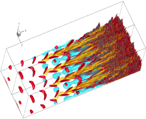
In the present paper, we present DNS and LES studies of Novec649 boundary-layer flows at conditions corresponding to the future wind tunnel set-up. One important motivation is to carry out a reference DNS for the spatial development of a boundary layer in realistic conditions. Our previous scale-resolving simulation in Sciacovelli et al. (Reference Sciacovelli, Gloerfelt, Passiatore, Cinnella and Grasso2020) used extreme conditions with an hypersonic Mach number and operating conditions inside the inversion zone of an heavy compounds (BZT conditions), to exacerbate dense-gas effects. In the present work, we aim at quantifying real-gas effects with milder conditions, representative of CLOWT facility and ORC applications. In particular, a modal transition is performed from a pair of oblique modes, determined from a preliminary linear stability study. The oblique ‘O-type’ scenario has been chosen since the initial perturbation is three-dimensional (3-D), which has been shown to be a key ingredient for transition (Klebanoff, Tidstrom & Sargent Reference Klebanoff, Tidstrom and Sargent1962). The role of TS waves is bypassed since low-speed streaks are rapidly generated and break down into turbulence by a lift-up mechanism (Waleffe Reference Waleffe1997). This scenario is similar to the late stages of FST-induced transition, where the laminar boundary layer develops high-amplitude, low-frequency perturbations (called Klebanoff mode) in response to FST forcing. We will thus achieve a controlled and orderly transition, that belongs to modal transition, which is pertinent for future studies of FST-induced transitions that preferentially occur in turbomachinery flows. We also vary the amplitude and frequency of oblique modes inducing the natural transition in order to determine when an equilibrium turbulent state is reached.
The paper is organised as follows. Governing equations and numerical methods are summarised in § 2, with special attention to the fluid models for Novec649. Compressible laminar boundary layers and their instabilities are discussed in § 3. Section 4 reports DNS results for transitional and fully turbulent states of a Novec649 boundary-layer flow at  $M=0.9$, $T_\infty =100\,^\circ {\rm C}$ and $p_\infty =4$ bars. The influence of the excitation parameters used to realise the modal transition are discussed in § 5 using LES.
2. Governing equations and gas model
2.1. Flow conservation equations
We consider flows of gases in the single-phase regime, governed by the compressible Navier–Stokes equations, written in differential form as
 \begin{gather} \frac{\partial\rho}{\partial t}+\frac{\partial(\rho u_j)}{\partial x_j} = 0 , \end{gather}
 \begin{gather}\frac{\partial(\rho u_i)}{\partial t}+\frac{\partial(\rho u_i u_j)}{\partial x_j}+ \frac{\partial p}{\partial x_i}-\frac{\partial\tau_{ij}}{\partial x_j} = 0 , \end{gather}
 \begin{gather}\frac{\partial(\rho E)}{\partial t}+\frac{\partial((\rho E + p) u_j)}{\partial x_j}- \frac{\partial(\tau_{ij}u_i)}{\partial x_j}+ \frac{\partial q_j}{\partial x_j} =0, \end{gather}
where  $x_i=(x,y,z)$ are the coordinates in the streamwise, wall-normal and spanwise directions, $u_i=(u,v,w)$ are the corresponding velocity components, $\rho$ is the density and $p$ the pressure. The specific total energy is $E\equiv e+u_ju_j/2$, $e$ being the specific internal energy, and the viscous stress tensor $\tau _{ij}$ is defined as
 \begin{equation} \tau_{ij}=\mu\left(\frac{\partial u_i}{\partial x_j}+\frac{\partial u_j}{\partial x_i}\right) +\mu'\frac{\partial u_k}{\partial x_k}\delta_{ij}, \end{equation}
where  $\mu$ is the dynamic viscosity and $\delta _{ij}$ denotes the Kronecker symbol. The second viscosity is set according to Stokes’ hypothesis, $\mu '=-2\mu /3$, assuming a zero bulk viscosity. This approximation is well verified for a dense gas as shown in Appendix B of Sciacovelli et al. (Reference Sciacovelli, Cinnella and Gloerfelt2017) or in Appendix C of Ren, Fu & Pecnik (Reference Ren, Fu and Pecnik2019). Finally, the heat flux is modelled by Fourier's law, $q_j=-\lambda (\partial T/\partial x_j)$, $\lambda$ being the thermal conductivity.
2.2. Fluid model for Novec649
In this study, the fluid is Novec649. It is the compound 1,1,1,2,2,4,5,5,5-nonafluoro-4-(trifluoromethyl)-3-pentanone, a perfluorinated ketone (chemical formula  ${\rm C}_6{\rm F}_{12}{\rm O})$ used as a working fluid in ORC, electronic cooling and fire suppression systems. Recent measurements (McLinden et al. Reference McLinden, Perkins, Lemmon and Fortin2015; Tanaka Reference Tanaka2016; Wen et al. Reference Wen, Meng, Huber and Wu2017; Perkins, Huber & Assael Reference Perkins, Huber and Assael2018) have been made to characterise its thermophysical properties. The values in table 1 are those given by the manufacturer (3M) and used in the NIST Refprop library (Lemmon, Huber & McLinden Reference Lemmon, Huber and McLinden2013).
Table 1. Main properties of Novec649 (from 3M). Here  $\mathcal {M}$ denotes the molar mass, $Z$ the compressibility factor, $R_g$ the individual gas constant, $c_{v,\infty }$ the ideal-gas specific heat at constant volume, $\bar {\omega }$ the acentric factor, $\bar {\xi }$ the dipole moment and subscript $c$ is used for critical conditions.

2.2.1. Equation of state for Novec649
The reference equation of state (EoS) in Refprop is based on experiments and modelling by McLinden et al. (Reference McLinden, Perkins, Lemmon and Fortin2015). Specifically, a multiparameter functional form based on the Helmholtz free energy is calibrated for Novec649, with estimated errors lower than 0.1 % for temperatures from 165 to 500 K and pressure up to 50 MPa. Additional measurements near the critical region were reported by Tanaka (Reference Tanaka2016) and underlined some uncertainties in the definition of the critical point.
In the present study, relatively dilute conditions for the vapour phase will be considered (see figure 1). A cubic EoS is chosen to reduce the overcost during the direct simulation integrations, namely the Peng & Robinson (Reference Peng and Robinson1976) EoS modified by Stryjek & Vera (Reference Stryjek and Vera1986) (hereafter abbreviated as PRSV). It is given as
 \begin{equation} p=\frac{R_g T}{{\mathcal{v}}-b}-\frac{a\alpha(T)}{{\mathcal{v}}^2+2b{\mathcal{v}}-b^2}, \end{equation}
where  $\mathcal {v}$ is the specific volume and $R_g$ the individual gas constant. By enforcing the critical-point conditions, the constants $a$,
$a$,  $b$ are given by
 \begin{equation} a=\underbrace{0.457235}_{a'}\frac{R_g^2T_c^2}{p_c}\quad b=\underbrace{0.077796}_{b'}\frac{R_g T_c}{p_c}\quad \alpha(T)=\left[1+K(1-\sqrt{T_r})\right]^2 \end{equation}
with  $T_r=T/T_c$ the reduced temperature. In the Stryjek & Vera (Reference Stryjek and Vera1986) modification, the parameter $K$ is $K_0+K_1(1+ \sqrt {T_r})(0.7-T_r)$ with $K_0=0.378893+1.4897153\bar {\omega }-0.17131848\bar {\omega }^2+0.196554\bar {\omega }^3$, $\bar {\omega }$ being the acentric factor. For $T_r>0.7$, the authors suggest that $K_1=0$, which is the case for our applications ( $T>310$ K). For cubic EoS, the critical quantities cannot be set independently and, introducing the compressibility factor $Z_c=p_c/(R_g\rho _c T_c)$, the compatibility at critical condition yields
 \begin{equation} 1=\frac{1}{Z_c-b'}-\frac{a'}{Z_c^2+2b'Z_c-b'^2}\quad\Rightarrow\quad Z_c\approx 0.3112. \end{equation}
Keeping reference values for  $T_c$ and $p_c$, the critical density is thus modified from its value in table 1 as $\rho _c=516.71\ \text {kg}\ \text {m}^{-3}$.

Figure 1. Clapeyron's diagram for Novec649. The thick black line represents the saturation curve and the thick dotted line marks the boundary of the dense-gas region ( $\varGamma <1$), where the colourmap represents values of the fundamental derivative of gas dynamics $\varGamma$. Isothermal curves obtained with PRSV EoS (thick solid red line) are compared with those obtained with the reference EoS of Refprop (thick dashed blue line). The hatched area indicates the limits of operability of CLOWT facility, and the three selected operating conditions A, B and C are marked with symbols.
For the calculation of caloric properties, the PRSV EoS is supplemented with a model for the ideal gas contribution to the specific heat at constant volume, represented by a power law of the form
 \begin{equation} c_{v,\infty}(T) = c_{v,\infty}(T_{c})\left(\frac{T}{T_{c}}\right)^n \end{equation}
where the exponent  $n$ is set at 0.405 and $c_{v,\infty }$ is given in table 1. The caloric EoS is then completely determined via the compatibility relation for the internal energy:
 \begin{equation} e = e_{ref} + \int_{T_{ref}}^T c_{v,\infty}(T') \,{\rm d}T' - \int_{\rho_{ref}}^{\rho} \left[ T\left.\frac{\partial p}{\partial T}\right|_{\rho} -p \right] \frac{{\rm d}\rho'}{\rho'^2}. \end{equation}
 The isothermal curves calculated with the reference EoS of Refprop and with PRSV EoS are compared in figure 1. A very good match is observed for dilute-gas conditions. The area of operation of CLOWT wind tunnel at Muenster University, namely  $p<1$ MPa and $T<453$ K (Reinker et al. Reference Reinker, Hasselmann, aus der Wiesche and Kenig2016), is indicated by the grayed region, which belongs to the dense-gas regime (fundamental derivative of gas dynamics, $\varGamma =1+\rho /c(\partial c/\partial \rho )_s<1$, $c$ being the sound speed and $s$ the entropy). Three operating conditions are selected in the following. Point A corresponds to nominal conditions of the future experimental campaign for Novec649 boundary layers, $p=4$ bars and $T=100\,^\circ {\rm C}$, and will be the operating point for the present DNS and LES study. Point B is chosen at the limits of operability of the CLOWT facility, which is still in the dilute-gas region. Finally, point C is close to the minimum of $\varGamma$, where greater non-ideal effects can be expected. Note that a minimum value of $\varGamma$ of 0.35 is estimated using PRSV EoS, meaning that Novec649 is not a BZT fluid (characterised by a region with $\varGamma <0$ in the vapour phase). The thermodynamic quantities obtained with PRSV and Refprop are reported in table 2. The difference is below 0.3 % for $p$,
$p$,  $T$,
$T$,  $\rho$ and up to 1 % for the sound speed $c$ at point C.
Table 2. Thermophysical properties at selected operating points A, B and C. Numbers in italic are imposed.

2.2.2. Transport properties for Novec649
Reference laws for Novec649 based on new measurements are implemented in the Refprop library (Lemmon et al. Reference Lemmon, Huber and McLinden2013), namely the model of Wen et al. (Reference Wen, Meng, Huber and Wu2017) for dynamic viscosity and the model of Perkins et al. (Reference Perkins, Huber and Assael2018) for thermal conductivity. In Wen et al. (Reference Wen, Meng, Huber and Wu2017), the viscosity correlation is written as a sum of three contributions:
 \begin{equation} \mu(\rho,T)=\mu_0(T)+\mu_1(T)\rho+\Delta\mu(\rho,T), \end{equation}
where  $\mu _0$ is the dilute-gas limit viscosity deduced from Chapman–Enskog theory (Chung et al. Reference Chung, Ajlan, Lee and Starling1988), $\mu _1(T)$ gives a density dependence of viscosity, following the work of Vogel et al. (Reference Vogel, Küchenmeister, Bich and Laesecke1998) and $\Delta \mu (\rho,T)$ is a residual term determined from an empirical fit based on measurements for the compressed liquid phase at pressures up to 40 MPa and a temperature range between 243 to 373 K. The estimated uncertainty of formula (2.10) is 2 % in this region. Unfortunately, there are no measurements in the gas phase, for which an uncertainty of 10 % is estimated (Lemmon et al. Reference Lemmon, Huber and McLinden2013).
In the present study, we use the viscosity model for dense gases of Chung, Lee & Starling (Reference Chung, Lee and Starling1984) and Chung et al. (Reference Chung, Ajlan, Lee and Starling1988), which is also based on a density-dependent correction of the Chapman–Enskog formula for pure substances and can be written as
 \begin{equation} \mu(\rho,T) = \mu_0(T) [1/G_2 + A_6 Y] + \mu_p(\rho,T), \end{equation}
where the dilute-gas component  $\mu _0$ is given by
 \begin{equation} \mu_0=4.0785\times 10^{{-}6}\frac{\sqrt{\mathcal{M}T}}{V_c^{2/3}\varOmega^*}F_c \quad\text{with}\ F_c=1-0.2756\bar{\omega}+0.059035\bar{\xi}_r^4,\end{equation} $\bar {\xi }_r=131.3\bar {\xi }/(V_cT_c)^{1/3}$ being the reduced dipole moment, and $V_c$ denoting the molar critical volume in ${\rm cm}^3\ {\rm mol}^{-1}$. The dimensionless Lennard–Jones collision integral $\varOmega ^*$ is approximated using the empirical equation of Neufeld, Janzen & Aziz (Reference Neufeld, Janzen and Aziz1972):
 \begin{align} \varOmega^*(T^*)&=1.16145(T^*)^{{-}0.14874}+0.52487\hbox{e}^{{-}0.7732T^*} +2.16178\hbox{e}^{{-}2.43787T^*}\nonumber\\ &\quad -6.435\times 10^{{-}4}(T^*)^{0.14874} \sin\left[18.0323(T^*)^{{-}0.7683}-7.27371\right] \end{align}
with  $T^*=1.2593 T/T_c$. A density dependence is introduced by the nonlinear function $G_2$:
 \begin{equation} G_2=\frac{A_1 [1-\exp{({-}A_4Y)}]/Y+A_2 G_1\exp{(A_5 Y)}+A_3 G_1}{A_1 A_4 + A_2 + A_3} \end{equation}
with
 \begin{equation} Y=\frac{\rho}{6 \rho_c},\quad G_1=\frac{1-0.5Y}{(1-Y)^3}. \end{equation}
The third term in (2.11) is a correction that takes into account dense-gas effects:
 \begin{equation} \mu_p=36.344\times 10^{{-}7}\frac{\sqrt{\mathcal{M}T_c}}{V_c^{2/3}} A_7 Y^2 G_2 \exp{[A_8 + A_9(T^*)^{{-}1} + A_{10}(T^*)^{{-}2}]}. \end{equation}
The constants  $A_1$– $A_{10}$ are functions of the acentric factor $\bar {\omega }$ and reduced dipole moment $\bar {\xi }_r$:
 \begin{equation} A_i=a_0(i)+a_1(i)\bar{\omega}+a_2(i)\bar{\xi}_r^4, \quad i\in\{1,\ldots,10\}, \end{equation}
whose coefficients  $a_0$, $a_1$ and $a_2$ are given in Chung et al. (Reference Chung, Ajlan, Lee and Starling1988) and in Appendix A of Sciacovelli et al. (Reference Sciacovelli, Cinnella and Gloerfelt2017).
For the thermal conductivity  $\lambda$, the correlation implemented in Refprop is that of Perkins et al. (Reference Perkins, Huber and Assael2018) based on measurements for vapour, liquid and supercritical fluid. It is made of three contributions:
 \begin{equation} \lambda(\rho,T)=\lambda_0(T)+\Delta\lambda_r(\rho,T)+\Delta\lambda_c(\rho,T). \end{equation}
A rational polynomial in reduced temperature  $T_r$ is used for the dilute-gas thermal conductivity $\lambda _0$ and a polynomial in temperature and density is fitted for the residual thermal conductivity $\Delta \lambda _r$. The last term $\Delta \lambda _c$ is used to describe the thermal conductivity enhancement in the critical region and relies on the crossover model of Olchowy & Sengers (Reference Olchowy and Sengers1988), which requires a model of viscosity (here the correlation of Wen et al. (Reference Wen, Meng, Huber and Wu2017)), and an EoS for heat capacities and density derivatives (here EoS of McLinden et al. Reference McLinden, Perkins, Lemmon and Fortin2015).
In our calculations, the Chung–Lee–Starling model (Chung et al. Reference Chung, Lee and Starling1984, Reference Chung, Ajlan, Lee and Starling1988) is used, which is written similarly to the viscosity model (2.11):
 \begin{equation} \lambda(\rho,T) = \lambda_0(T) [1/H_2 + B_6 Y] + \lambda_p(\rho,T). \end{equation}
The dilute-gas contribution  $\lambda _0$ is modelled as
 \begin{equation} \lambda_0=418.4\times 7.452\frac{\mu_0}{\mathcal{M}}\psi, \end{equation}
where  $\mu _0$ is given by (2.12) and $\psi$ is a modified Eucken-type correlation based on kinetic theory extended to polyatomic gases, where the contribution of internal degrees of freedom (rotational and vibrational) is added to translational degrees of freedom:
 \begin{equation} \psi=1+\alpha\frac{0.215+0.28288\alpha-1.061\beta+0.26665 Z_{{coll}}} {0.6366+\beta Z_{{coll}}+1.061\alpha\beta}, \end{equation}
with a rotational coefficient  $\alpha =c_{v,\infty }/R_g-3/2$, a diffusion term $\beta$, empirically linked to the acentric factor as $\beta =0.7862-0.7109\bar {\omega }+1.3168\bar {\omega }^2$ and $Z_{{coll}}=2+10.5 T_r^2$ modelling the number of collisions required to interchange a quantum of rotational energy with translational energy. In the same way as the viscosity model, the dilute-gas contribution is weighted by a density-dependent nonlinear term $H_2$, given by
 \begin{equation} H_2=\frac{B_1 [1-\exp{({-}B_4Y)}]/Y+B_2 G_1\exp(B_5 Y)+B_3 G_1}{B_1 B_4 + B_2 + B_3}, \end{equation}
with  $Y$ and $G_1$ defined by (2.15a,b). The third term in (2.11) is a dense-gas correction:
 \begin{equation} \lambda_p=418.4\times 3.039\times 10^{{-}4}\frac{\sqrt{T_c/\mathcal{M}}}{V_c^{2/3}} B_7 Y^2 H_2 T_r^{1/2}. \end{equation}
The constants  $B_1$– $B_7$ are functions of the acentric factor $\bar {\omega }$ and reduced dipole moment $\bar {\xi }_r$:
 \begin{equation} B_i=b_0(i)+b_1(i)\bar{\omega}+b_2(i)\bar{\xi}_r^4, \quad i\in\{1,\ldots,7\}, \end{equation}
with coefficients  $b_0$, $b_1$ and $b_2$ given in Chung et al. (Reference Chung, Ajlan, Lee and Starling1988).
The transport properties calculated with Chung–Lee–Starling and Refprop models for selected operating conditions A, B and C are reported in table 2. The difference for viscosity values decreases from 30 % (point A) to 6 % (point C). A difference of about 15 % is noted for the thermal conductivity. Since the dilute-gas component  $\mu _0(T)$ is the same in the models of Wen et al. (Reference Wen, Meng, Huber and Wu2017) and Chung et al. (Reference Chung, Ajlan, Lee and Starling1988), this means that the differences observed for the viscosity are due to the density dependence, even in the very dilute condition (point A). A posteriori validations for the laminar boundary layer are reported in § 3.1.
2.3. Flow solver
The in-house finite-difference code Musicaa is used to solve the compressible Navier–Stokes equations (2.1)–(2.3). The inviscid fluxes are discretised by means of tenth-order standard centred differences whereas fourth order is used for viscous fluxes. The scheme is supplemented with a tenth-order selective filtering to eliminate grid-to-grid unresolved oscillations. A four-stage Runge–Kutta algorithm is used for time integration. The implicit residual smoothing (IRS) method of Cinnella & Content (Reference Cinnella and Content2016), modified in Bienner, Gloerfelt & Cinnella (Reference Bienner, Gloerfelt and Cinnella2022a), can be used to enlarge the stability domain and enable the use of larger time steps. Adiabatic no-slip conditions are applied at the wall, and non-reflecting Tam and Dong's conditions are imposed at the inlet, top and outflow boundaries. A sponge zone combining grid stretching and a Laplacian filter is added at the outlet. Periodicity is enforced in the spanwise direction.
The in-house flow solver has already been used in the past for fundamental study of wall-bounded flows of the heavy fluorocarbon PP11, namely channel flow (Sciacovelli et al. Reference Sciacovelli, Cinnella and Gloerfelt2017) and supersonic boundary layers (Sciacovelli et al. Reference Sciacovelli, Gloerfelt, Passiatore, Cinnella and Grasso2020).
2.4. Linear stability solver
The local stability analysis is based on the linearised compressible Navier–Stokes equations written in Cartesian coordinates. The local assumption imposes that the base flow is a function of the crossflow dimension  $y$ solely. The latter is obtained from the similarity solution of a zero-pressure-gradient compressible laminar boundary layer generalised to fluids governed by an arbitrary EoS (Gloerfelt et al. Reference Gloerfelt, Robinet, Sciacovelli, Cinnella and Grasso2020). The differential eigenvalue problem is solved using the Chebyshev collocation method (see Gloerfelt & Robinet (Reference Gloerfelt and Robinet2017) and Gloerfelt et al. (Reference Gloerfelt, Robinet, Sciacovelli, Cinnella and Grasso2020) for details about the stability solver and its extension to dense gases). 3-D spatial modes are searched with a real angular frequency $\omega$ and a complex wavenumber $\boldsymbol {k}=\alpha \boldsymbol {e}_x+\beta \boldsymbol {e}_z$. The streamwise component of the wavenumber is a complex number, $\alpha = \alpha _r + {\rm i}\alpha _i$, where $\alpha _i$ thus represents the amplification factor. The spanwise component $\beta$ defines the wave angle $\varPsi =\arctan (\beta /\alpha _r)$.
3. Laminar boundary layers of Novec649
3.1. Influence of operating conditions
The similarity solutions for a zero-pressure-gradient compressible laminar boundary layer are computed for the three operating points A, B and C defined in the previous section (see table 2) and a Mach number  $M=0.9$. The results are given in figure 2 and table 3. The similarity solutions obtained with the Peng–Robinson–Stryjek–Vera (PRSV) EoS and Chung–Lee–Starling transport properties are compared with those for the reference laws available in Refprop. The velocity profiles are all superimposed, meaning that the operating conditions and/or the fluid models have a weak influence. Small deviations are observed for the temperature profiles in figure 2. The wall temperature, reported in table 3, is slightly underestimated ( $-$0.05 %) for point A and overestimated for point C ( $+$0.023 %). Greater discrepancies are visible for the dynamic viscosity profiles, as already discussed in § 2.2. The maximum deviation for point C is 1.4 %. It is worth noting that a gas-like behaviour (increasing viscosity with increasing temperature) is obtained for the more dilute condition C, whereas viscosity follows a liquid-like behaviour for the two other points (more pronounced for point A, close to the minimum of $\varGamma$). This behaviour is captured by both fluid models. At the high subsonic Mach number under consideration ( $M=0.9$) the friction heating is negligible (less than 1 %) due to the high heat capacity of Novec649. For comparison, temperature variations of 14 % are obtained in air for this Mach number. As a consequence, the thickening factor $\delta ^*/L^*\approx 1.74$ is very close to the incompressible value of 1.72, where $\delta ^*$ denotes the displacement thickness and $L^*$ the Blasius length scale $\sqrt {\mu _\infty x/(\rho _\infty U_{\infty })}$.

Figure 2. Influence of operating conditions on a laminar boundary layer at  $M=0.9$. Non-dimensional streamwise velocity, temperature and viscosity: similarity solutions using PRSV/Chung–Lee–Starling (solid lines) and Refprop laws (dashed lines).
Table 3. Influence of operating conditions on a laminar boundary layer at  $M=0.9$. Properties at points A, B and C from similarity solutions.

To investigate the influence of the fluid models on the development of unstable modes in the laminar boundary layer, a two-dimensional (2-D) linear stability analysis is conducted for the three operating conditions. The neutral curves obtained for PRSV/Chung and Refprop models are almost superimposed in figure 3. The amplification factor obtained at  $Re_{L^*}=2000$ is plotted in the left panel, and only the enlarged view in the inset shows weak variations, with slightly more unstable waves for dilute conditions and for Refprop models with respect to PRSV/Chung models. The deviations for the maximum amplification are always lower than 1 %.

Figure 3. Influence of operating conditions on instabilities at  $M=0.9$. Neutral curves on the left and growth rate at $Re_{L^*}=2000$ on the right for various base flows: similarity solutions using PRSV/Chung–Lee–Starling (solid lines) and Refprop laws (dashed lines).
3.2. Influence of Mach number
To better understand the unstable modes for Novec649 boundary layers, the effect of the Mach number is then explored. Since the influence of the operating conditions is moderate, at least at high subsonic Mach number, the thermodynamic properties are those of point C (4 bar and  $100\,^\circ {\rm C}$), to be used in experiments and in the forthcoming turbulent simulations. First, base flows are computed using the similarity solutions for Mach numbers between 0.3 and 6. The characteristics of the various computed cases are summarised in table 4 and some profiles are displayed in figure 4. The maximum value of the fundamental derivative $\varGamma$ at the wall is reached for the highest Mach number and stays below one. Friction heating remains limited for Novec649, with a maximum wall overheat of 31 % at $M=6$, whereas a factor greater than 7 would be obtained for air at the same Mach number. A similar parametric study was carried out for a heavier fluorocarbon (PP11, ${\mathcal {M}}=624\ {\rm g}\ {\rm mol}^{-1}$) and a lighter refrigerant (R134a, ${\mathcal {M}}=102\ {\rm g}\ {\rm mol}^{-1}$) in Gloerfelt et al. (Reference Gloerfelt, Robinet, Sciacovelli, Cinnella and Grasso2020). An overheat of 2.5 % were obtained for PP11 and 34.5 % for R134a. As a consequence, the longitudinal velocity profiles for Novec649 remain close to the incompressible one up to $M=3$ and progressively thicken due to friction heating. However, even at $M=6$, the increase of the boundary layer thickness is only 15 % (for comparison, a factor of 20 can be obtained in air). The viscosity profiles in figure 4(c) follow the temperature distributions (gas-like behaviour). The non-dimensional generalised derivative $({L^*}^2/(\rho _\infty U_\infty ))\partial (\rho \partial u/\partial y)/\partial y$ is plotted in figure 4(d) as a function of $y/\delta$. Lees & Lin (Reference Lees and Lin1946) demonstrated that it gives a necessary condition for a compressible boundary-layer flow to be inviscidly unstable. For air, a generalised inflection point appear for supersonic flows at a distance from the wall that increases as $M$ increases, such that the instability becomes progressively inviscid for $M\gtrapprox 3$. For a heavy dense gas, such as PP11, the generalised inflection point is absent (Gloerfelt et al. Reference Gloerfelt, Robinet, Sciacovelli, Cinnella and Grasso2020). For the present organic vapour, a weak generalised inflection point is present for $M\gtrapprox 3$ but it remains very close to the wall. As a consequence, the inviscid mechanism does not take over, and the TS-like mode is continuously damped by compressibility effects.

Figure 4. Influence of Mach number at flow conditions corresponding to point C ( $T_\infty =100\,^\circ {\rm C}, p_\infty =4$ bars): (a) streamwise velocity, (b) temperature, (c) viscosity and (d) non-dimensional generalised derivatives profiles. Line legend as in table 4.
Table 4. Influence of Mach number: boundary layer properties from similarity solutions.

The growth rates  $\alpha _i$, obtained with 2-D spatial LST at $Re_{L^*}=2000$, are plotted in figure 5(a) for the various Mach numbers (line legend in table 4). Two sets of results are well separated. In the low-frequency range, typically $\omega L^*/U_\infty \lessapprox 0.05$, the first mode occurs, which is the continuation of the viscous TS instability. In the high-frequency range, a strong instability arises for $M\gtrapprox 2.5$. Its nature is very different and is discussed later for $M=6$ (see also Gloerfelt et al. Reference Gloerfelt, Robinet, Sciacovelli, Cinnella and Grasso2020). The evolution of the first mode with the Mach number is first scrutinised in figure 5(b). For subsonic flows, the 2-D viscous mode is similar to the TS instability, with a maximum amplification around a non-dimensional frequency of 0.03, and it is progressively damped as the flow becomes supersonic. The 2-D waves are marginally unstable for $M=1.5$ and become stable above since the generalised inflection is either too weak or too close to the wall. To counter the stabilising effect of increasing speeds, viscous instabilities will develop preferentially with an obliqueness angle that reduces their relative phase speed.

Figure 5. Influence of Mach number on the growth rate of 2-D instabilities at  $Re_{L^*}=2000$. (a) Global view and (b) successive close-up views of the TS instabilities. Line legend as in table 4.
In figure 6, we report the growth rates and phase speeds for  $M=6$. As first brought to light by Mack (Reference Mack1963, Reference Mack1984), when a region of the mean flow becomes supersonic relative to the phase speed of the modes, typically for $M>4$, multiple acoustic modes can occur. The denomination ‘acoustic’ refers to the presence of sound waves reflected back and forth between the wall and the sonic line. As shown in Gloerfelt et al. (Reference Gloerfelt, Robinet, Sciacovelli, Cinnella and Grasso2020), the fact that the friction heating is dramatically reduced for a dense gas entails a thinner boundary and a thinner height of the acoustic wave guide. As a consequence, the acoustic wavelength is reduced and the acoustic mode is moved towards high frequencies (a similar mechanism exists for cold walls). In this frequency range, the eigenvalue, giving rise to the first mode, called mode S because it comes from the slow acoustic branch (Fedorov & Tumin Reference Fedorov and Tumin2011), is strongly stable. The terminology is more explicit by looking at the phase speed in figure 6(b). At $\omega =0$ (leading edge), mode S has a phase speed $U-c$ (slow acoustic waves). Other modes correspond to eigenvalues with phase speed $U+c$ at the leading edge (fast modes) and are thus referred to as modes F $_1$,
$_1$,  ${\rm F}_2$, $\ldots$. In figure 6(a), the unstable acoustic mode arises first from mode F $_1$. After the maximum amplification, near $\omega L^*/U_\infty \approx 0.3$, a kink is visible that corresponds to the frequency where F $_1$ phase speed has decreased below $1-1/M$ and, thus, becomes supersonic. Such a mode is called a supersonic mode. As it stabilises, the eigenvalue crosses the slow acoustic branch (located on the real axis) leading to the discontinuity observed in figure 5(a). In fact, after the branch cut, a new eigenvalue (noted F $_1^-$) occurs. This phenomenon is similar to the synchronisation with the entropy/vorticity branch, well described in Fedorov & Tumin (Reference Fedorov and Tumin2011) or Ren & Fu (Reference Ren and Fu2015). Similar results were obtained for other dense gases in Gloerfelt et al. (Reference Gloerfelt, Robinet, Sciacovelli, Cinnella and Grasso2020). Interestingly, for Novec649, the next acoustic mode F $_2$ (two wavelengths in the waveguide) can also become unstable, which was not observed previously and can only exist in air for high-enthalpy cold-wall boundary layers at very high speeds. Even if the main mechanism are similar among various dense gases, the peculiar behaviour of each compound, such as the onset $M$ of the supersonic mode, can be related to their sound speed that modifies the resonance frequency of acoustic waves.

Figure 6. (a) Growth rate and (b) phase speed at  $M=6$ and $Re_{L^*}=2000$.
The 3-D instabilities are studied by varying the wave angle  $\varPsi$ (or, equivalently, the spanwise wavelength). As already pointed out, at supersonic speeds, oblique waves can take over 2-D modes. In figure 7(a), the maximum growth rate of 2-D waves is at $\varPsi =0^\circ$ up to $M=0.9$. From $M=1.2$ to 1.5, the 2-D wave is still unstable but the maximum amplification occurs for increasing wave angle (49 and $62^\circ$ respectively). For $M$ around 2, of interest for supersonic ORC turbine flows, the 2-D modes are stable and the most unstable waves are oblique modes with $\varPsi \sim 65^\circ$ ( $62.6^\circ$ at $M=1.8$ and $66.4^\circ$ at $M=2.1$). Note that the angular frequency at which the maximum is reached is different from the frequency of the most unstable 2-D waves. This is illustrated in figure 7(b) for $M=1.5$. In the $\omega$– $\varPsi$ plane, the thin dashed line corresponds to the maximal 2-D growth, whereas the thick dashed line marks the location of the maximal 3-D growth. A similar map for $M=2.1$ in figure 7(c) shows that large wave angles ( ${\gtrapprox }40^\circ$) are necessary for the mode destabilisation.

Figure 7. Influence of Mach number on 3-D instabilities at  $Re_{L^*}=2000$. Growth rate as a function of wave angle $\varPsi$ in degrees (a) at the frequency of maximal 2-D growth rate for $M<1.5$ ( $\omega L^*/U_\infty =0.0314$ at $M=0.5$; 0.0294 at $M=0.6$; 0.0262 at $M=0.9$; and 0.0216 at $M=1.2$) and at the frequency corresponding to the maximal 3-D growth for $M\ge 1.5$ ( $\omega L^*/U_\infty =0.0195$ at $M=1.5$; 0.0177 at $M=1.8$; and 0.016 at $M=2.1$). Bullets mark the most unstable 3-D waves, if one exists. Examples of $\varPsi$– $\omega$ maps for (b) $M=1.5$ and (c) $M=2.1$ used to determine the frequency of the maximal 3-D growth. Levels of $\alpha _i L^*$ are between $-3\times 10^{-3}$ (respectively, $-2\times 10^{-3}$) and 0 (white) for $M=1.5$ (respectively, $M=2.1$). The thick green dashed lines mark the location of the maximal 3-D growth, whereas the thin green dashed line indicates the maximal 2-D growth for $M=1.5$.
Finally, the linear stability analysis is carried out to determine the most unstable oblique modes at  $M=0.9$, which will be used to trigger transition towards the turbulent regime in the following. Neutral curves are displayed in figure 8(a) for wave angle between $0^\circ$ (2-D) and $50^\circ$. The 2-D waves are the most unstable since the flow is subsonic but, for low values of $\varPsi$, the 3-D modes are almost as unstable as their 2-D counterpart, notably for low frequencies. In the following study, we have chosen $\varPsi =30^\circ$ for the oblique modes (red dashed curve in the figure). Figure 8(b) shows the amplification rate $\alpha _i L^*$ bounded by the neutral curve (negative values denote unstable waves) using the non-dimensional frequency $F=\omega \mu _\infty /(\rho _\infty {U_\infty }^2)$. Since $\omega L^*/U_\infty =Re_{L^*} F$, the path followed by DNS and LES simulations are represented by horizontal lines. For instance, the nominal DNS and LES calculations will start at $Re_{L^*}=1000$ with an angular frequency $\omega L^*/U_\infty =0.02$, corresponding to the green dashed line $F=2\times 10^{-5}$. Two other frequencies will also be examined, namely $\omega L^*/U_\infty =0.024$ (blue dashed line) and $\omega L^*/U_\infty =0.04$ (magenta dashed line). Finally, the neutral curve obtained for air (with stagnation temperature and pressure of 305 K and 0.819 atm, respectively) is plotted with a dotted line for comparison. The shape and the stability bounds are relatively similar (due to the very close velocity profile) but the Novec649 boundary layer is slightly more stable.

Figure 8. Oblique modes at  $M = 0.9$. (a) Neutral curves for various values of the wave angle $\varPsi$. The selected values $\varPsi =30^\circ$ corresponds to the red dashes. (b) $F$–
$F$– $Re$ map of amplification rate at $\varPsi = 30^\circ$ for Novec649 (thick solid black line) and for air (black small dotted squares). The DNS and LES simulation paths are shown with horizontal dashed lines.
3.3. Simulation of 2-D instabilities
The development of 2-D TS-like instabilities at  $M=0.9$ is simulated using the DNS code for various initial wave amplitudes. The computational domain is discretised by $2000\times 400$ points, with $\Delta x=4\times 10^{-6}$ m and $\Delta y_w=10^{-7}$ m. The inlet plane corresponds to $Re_{L^*}=1000$, where 2-D instabilities from LST are imposed at an angular frequency $\omega _0 L^*/U_\infty =0.02$. The mode obtained from LST has a wavenumber $\alpha _r L^*=0.06486$ and a growth rate $\alpha _i L^*=-2.7\times 10^{-4}$ (almost neutral). The wavelength of the perturbation $\lambda _x=2{\rm \pi} /\alpha _r=96.87 L^*$ is discretised by $84\Delta x$. Since the DNS results will be Fourier transformed in time to get the harmonic contribution at the forcing frequency, the time step is fixed as $\Delta t=2{\rm \pi} /\omega _0/23\,000$, yielding a Courant–Friedrichs–Lewy (CFL) number of approximately 1. At such conditions, the simulations are conducted using an explicit time stepping. First, a precursor calculation of 1 500 000 iterations without the excitation is run to generate the base flow. When non-dimensionalised with free-stream quantities (subscript $\infty$) and the Blasius length scale $L^*$, perfectly autosimilar profiles are obtained in figure 9 in excellent agreement with the similarity solution.

Figure 9. Laminar boundary layer of Novec649 at  $M=0.9$. Non-dimensional streamwise velocity, temperature and wall-normal velocity: DNS profiles (thick solid green line) compared with similarity solutions using PRSV/Chung–Lee–Starling (circles).
The simulation is then run for 500 000 iterations with the LST eigenfunctions for  $u$,
$u$,  $v$,
$v$,  $p$,
$p$,  $\rho$ and $T$ imposed in the Tam & Dong inflow condition (Gloerfelt & Robinet Reference Gloerfelt and Robinet2017). Since the stability analysis is linear, we need to prescribe an amplitude for the inlet perturbations. We select four values from $\varepsilon _0=10^{-4} U_\infty$, which ensures that the disturbance stays in the linear regime, up to $\varepsilon _0=5\times 10^{-3} U_\infty$. The results are stored for the last 23 000 iterations every 100, which corresponds to one period. The amplitude $A_1(x)$ of the Fourier transform of the wall pressure at the fundamental frequency is used to compute the spatial growth rate as $\alpha _i=-{\rm d}[\ln (A_1(x))]/{{\rm d}x}$. Figure 10(a) shows the streamwise evolution of the computed growth rate compared with LST results as a function of Blasius Reynolds number (bottom scale) and distance $x$ (top scale). After slight oscillations due to the adaptation of the inflow boundary condition, the growth rate for $\varepsilon _0=10^{-4} U_\infty$ is in fair agreement with the LST results all along the computational box. The maximum growth rate computed from DNS is slightly higher, which can be attributed to non-parallel effects ignored in the LST. As the forcing amplitude is increased, the growth rate deviates more and more rapidly from the LST curve, highlighting the onset of nonlinearities that saturate earlier the unstable mode. At the highest value ( $\varepsilon _0=5\times 10^{-3} U_\infty$), the saturation is almost immediate and strong oscillations of $\alpha _i$ are visible. The amplitude and phase of the DNS modes for $\varepsilon _0/U_\infty =10^{-4}$ and $10^{-3}$ are compared in figure 10(b) with LST at the location $Re_{L^*}=1200$. The profiles for both amplitudes match perfectly and the modulus and phase of the simulated waves are in fair agreement with LST. Once again, the discrepancies can be attributed to non-parallel effects present in DNS but not to the chosen forcing amplitude. These preliminary results also validate the use of the DNS code to simulate the linear development of instabilities.

Figure 10. DNS of 2-D TS waves. (a) Growth rate from DNS with various amplitudes ( $\varepsilon /U_\infty =10^{-4}$, dark orange dashed line; $5\times 10^{-4}$, light blue dashed line; $10^{-3}$, green dashed dot line; $5\times 10^{-3}$, dark purple dashed line) compared with LST (black solid line). (b) Amplitude (top row) and phase (bottom row) at $Re_{L^*}=1200$ of the streamwise velocity, wall-normal velocity and pressure disturbances from DNS ( $\varepsilon /U_\infty =10^{-4}$, dark orange line; $10^{-3}$, green dashed dot line) compared with LST (black solid line).
4. DNS of a turbulent boundary-layer flow of Novec649 at  $M=0.9$

4.1. DNS set-up
Boundary layer modal transition from the laminar to the fully turbulent regime in Novec649 is first carried out by means of DNS. The thermodynamic operating conditions correspond to the nominal case in § 3.1, namely a free-stream temperature  $T=100\,^\circ {\rm C}$ and pressure $p=4$ bars, and the Mach number is $M=0.9$, as in the future experimental campaign in the CLOWT facility. To induce a relatively rapid transition, a pair of unstable oblique modes, determined in the previous section, are entered with an amplitude $\varepsilon =10^{-3}U_\infty$. At the inlet, where the Reynolds number is $Re_{L^*}=1000$, oblique waves skewed by $30^\circ$ with respect to the mean-flow direction are imposed at a non-dimensional angular frequency $\omega _0 L^*/U_\infty =0.02$. The spanwise extent is taken equal to one wavelength of the input modes, $\lambda _z=2{\rm \pi} /\beta _0$, with the spanwise wavenumber $\beta _0=0.04 L^*$. The path followed by the DNS is shown with the green dashed line in figure 8.
A grid of  $9000\times 400\times 1000$ points (3.6 billion) is used, yielding a DNS resolution with mesh sizes in wall units ( $\Delta x_i^+=\Delta x_i u_\tau /\nu$, $u_\tau$ being the friction velocity and $\nu$ the kinematic viscosity) equal to ${\rm \Delta} x^+=15.7$–12.9 in the streamwise direction, $\Delta z^+=7.7$–6.3 in the spanwise direction, and $\Delta y^+_w=0.78$–0.64 at the wall and $\Delta y^+_e=12.2$–10.7 at the boundary-layer edge over the turbulent region. The simulation is run for 500 000 iterations with a maximum ${\rm CFL}=1$ and the explicit Runge–Kutta time stepping, and then statistics are collected during 450 000 iterations. The overall cost is approximately 5 million CPU hours on 18 000 CascadeLake cores.
4.2. Oblique breakdown
A snapshot of the DNS is shown in figure 11. The axes are kept dimensional and the portion of the flat plate simulated is just over a centimeter long (the experiments in CLOWT facility will use a plate of 6 cm). Transition to turbulence is seen to occur 3 mm from the plate leading edge and boundary layer thickness is of the order of one-tenth of millimetre. Measurements are thus very challenging, especially as the high density of Novec649 precludes the use of miniaturised hot wire.

Figure 11. Instantaneous views of the streamwise velocity ( ${\rm m}\ {\rm s}^{-1}$) (a) in the plane $z=0$ and (b) in the plane $y^+\approx 15$.
A 3-D view of the transitional region is reported in figure 12. A checkerboard pattern is visible just after the inlet due to the interaction of the two initial oblique waves with opposite angles (see also figure 24 in § 5). Further downstream, the initial oblique modes  $(\omega /\omega _0,\beta /\beta _0)=(1,\pm 1)$ grow slowly. From 2-D results of figure 10, the onset of nonlinear saturation due to the forcing amplitude is expected to occur after $x=2$ mm. In 3-D, the $\lambda _2$-criterion clearly shows saturated vortices as early as $x=1$ mm, meaning that the forcing amplitude is not directly responsible for the early nonlinear energy transfer between modes. Using a 2-D $t$–
$t$– $z$ Fourier transform of the streamwise velocity component in the horizontal plane $y=0.0013$ mm, the development of the ( $\omega /\omega _0,\beta /\beta _0$) modes is obtained in figure 13. Initially, the only present mode is $(1,\pm 1)$ but the first streak mode $(0,2)$ rapidly emerges near $x=0.5$ mm and dominates after $x=0.7$ mm. This mode is represented by isocontours of the fluctuating streamwise velocity in the 3-D view of figure 12, which correspond to laminar streaks of opposite sign, visible from $x=1$ mm with the selected isocontour level. The latter are modulated by the checkerboard pattern in their early development. The mode $(1,3)$, resulting from nonlinear interactions with the fundamental oblique waves, reaches a large amplitude at $x=1$ mm. Nonlinearities then rapidly develop with the eruption of streak harmonics $(0,4)$ and $(0,6)$. These wavelength doublings are better identified on top views of the fluctuating velocity (see figures 24 or 34 in § 5). This first phase is very similar to the observations for oblique transition from the literature (Elofsson & Alfredsson Reference Elofsson and Alfredsson1998; Berlin, Wiegel & Henningson Reference Berlin, Wiegel and Henningson1999; Gloerfelt & Robinet Reference Gloerfelt and Robinet2017). The low-speed streaks have a sinuous evolution and the appearance of high frequencies due to transient growth leads rapidly to turbulence.

Figure 12. Instantaneous view of the transitional region: two isocontours of the fluctuating longitudinal velocity ( $u'=0.05\ {\rm m}\ {\rm s}^{-1}$ in yellow and $u'=-0.05\ {\rm m}\ {\rm s}^{-1}$ in blue) and one isocontour of $\lambda _2$-criterion ( $\lambda _2\delta _{1,in}^2/U_\infty ^2=-1.26\times 10^{-8}$ in red). The domain is duplicated in the spanwise direction.

Figure 13. Streamwise evolution of Fourier components with frequency and spanwise wavenumber ( $\omega /\omega _0,\beta /\beta _0$) for the streamwise velocity at $y=0.0013$ mm.
4.3. Fully turbulent state
The evolution of the skin friction coefficient  $C_f=\tau _w/(\frac {1}{2}\rho _\infty U_\infty )$ is plotted in figure 14(a) with the wall shear stress evaluated as $\tau _w=\bar {\mu }_w(\partial \bar {u}/\partial y)_w$. The friction coefficient departs rapidly from the laminar correlation and is found to be in very good agreement with incompressible DNS databases (Wu & Moin Reference Wu and Moin2009; Schlatter & Örlü Reference Schlatter and Örlü2010) further downstream, meaning that a canonical zero-pressure-gradient turbulent boundary layer is obtained for a range of Reynolds numbers $Re_\theta$, based on momentum thickness, between approximately 1500 and 5000. Almost no overshoot of the friction coefficient is observed here, which is reminiscent to the FST-induced bypass transition of Wu & Moin (Reference Wu and Moin2009), even if the Reynolds number of transition is larger since the inlet Reynolds number is relatively high. A similar zero-pressure-gradient boundary layer at $M=0.9$ in air would correspond to smaller values of $C_f$ due to friction heating effects, as illustrated by the data from Wenzel et al. (Reference Wenzel, Selent, Kloker and Rist2018). This effects can be physically interpreted as an incompressible $C_f$-distribution that is stretched by compressibility and viscosity effects. For the dense gas, since the wall temperature differs by less than 1 %, compressibility effects on the mean flow are almost absent.

Figure 14. (a) Skin friction coefficient: present DNS (thick solid black line); incompressible DNS of Schlatter & Örlü (Reference Schlatter and Örlü2010) (blue circles); DNS of bypass transition of Wu & Moin (Reference Wu and Moin2009) (red squares); compressible DNS of Wenzel et al. (Reference Wenzel, Selent, Kloker and Rist2018) at  $M=0.85$ (down triangles); laminar Blasius correlation $0.664/\sqrt {Re_x}$ (blue squares). (b) Mean streamwise velocity at $Re_\theta =2000$, 2540, 3030, 3270, 3630, 3970 and 4060 (solid lines from red to blue) compared with DNS results of Schlatter & Örlü (Reference Schlatter and Örlü2010) (dashed lines) at the same $Re_\theta$.
Figures 14(b) and 15 show the mean streamwise velocity profiles  $\bar {u}^+=\bar {u}/u_\tau$ and turbulent intensities $u^+_{i,rms}=u_{i,rms}/u_\tau$ (where $u_i$ is either the streamwise $u$, wall-normal $v$ or transverse $w$ components of the velocity vector and the friction velocity is $u_\tau =\sqrt {\tau _w/\bar {\rho }_w}$) for various streamwise stations. The profiles are in good agreement with the incompressible database of Schlatter & Örlü (Reference Schlatter and Örlü2010) at the same values of $Re_\theta$. Slight deviations can be seen for the first station, where the Novec649 boundary layer has not yet reached a perfect turbulent equilibrium.

Figure 15. Turbulent intensity profiles at  $Re_\theta =2000$, 2540, 3030, 3270, 3630, 3970 and 4060 (solid lines from red to blue) compared with Schlatter & Örlü (Reference Schlatter and Örlü2010) (dashed lines).
The turbulent kinetic energy (TKE) budget, written in the compressible regime, is reported in figure 16. The main terms of the budget are the production term  $(- \overline {\rho u_i''u_j''}({\partial \tilde {u}_i}/{\partial x_j}))$, the turbulent transport term $(-\frac {1}{2}({\partial }/{\partial x_j})\overline {\rho u_i''^2u_j''}-({\partial }/{\partial x_j})\overline {p'u_i'} )$, the viscous diffusion term $({\partial }/{\partial x_j}) \overline {u_i'\tau _{ij}})$ and the viscous dissipation term $(-\overline {\tau _{ij}({\partial u_i'}/{\partial x_j}}))$. Here the compressible form (Bogey & Bailly Reference Bogey and Bailly2009) is implemented with $(\overline {\cdot })$ the Reynolds average and $(\widetilde {\cdot })$ the Favre average; prime quantities are Reynolds fluctuations and double prime Favre fluctuations. Note that Reynolds and Favre averaging provide essentially the same results at the present Mach number, with velocity statistics very close to the incompressible ones. These terms, normalised by $\bar {\rho }_w u_\tau ^4/\bar {\nu }_w$, are in very good agreement with incompressible DNS databases at $Re_\theta \approx 4000$.

Figure 16. TKE budget: production (thick blue solid line); turbulent transport (thick black solid line); viscous diffusion (thick cyan solid line); viscous dissipation (thick solid green line); pressure dilation  $+$ pressure diffusion (thick magenta solid line); mean flow convection (thick red solid line). Solid lines denote the present DNS at $Re_{\theta }=4060$ compared with incompressible DNS of Schlatter & Örlü (Reference Schlatter and Örlü2010) at $Re_\theta =4060$ (circles) and Sillero, Jimenez & Moser (Reference Sillero, Jimenez and Moser2013) at $Re_\theta =4000$ (asterisks).
In figure 17, premultiplied spanwise energy spectra are shown for the streamwise velocity at  $Re_\theta =2435$ and 4963. An invariant maximum is found at a wall distance of $y^+=12$ with a wavelength $\lambda _z^+=120$, corresponding to near-wall turbulent streaks. These values are the same as those observed for incompressible boundary layer (Schlatter et al. Reference Schlatter, Li, Brethouwer, Johansson and Hennigson2010; Eitel-Amor, Örlü & Schlatter Reference Eitel-Amor, Örlü and Schlatter2014). For sufficiently high Reynolds numbers, a second peak emerges due to the presence of large scales in the outer region, whose location and wavelengths scaled in outer units are $y\approx 0.13\delta$ and $\lambda _z\approx 0.7\delta$, respectively. The emergence of large-scale motions is also present in the temporal spectra of figure 18. To obtain spectral information, the temporal signal, made of 9000 samples recorded every $50\Delta t_{{DNS}}$, is transformed in Fourier space using the spectral estimator of Capon (Reference Capon1969) and the Welch method with Hann windowing and 4 overlapping segments. The frequency resolution is 22.3 kHz. Contour plots of the premultiplied temporal spectra for two values of the Reynolds number show that a broad range of temporal frequencies are excited with dominant activity for $\lambda _t U_\infty /\delta$ between 1 and 3 in the near-wall region ( $y^+\approx 15$). As the Reynolds is increased, spectral level are more intense for large wavelengths in the outer region ( $y>0.1\delta$), indicating the presence of longer lasting structures. Using a Taylor's hypothesis, this indicates the presence of elongated large-scale motions. Using a convection velocity $U_c=0.7U_\infty$, the temporal scales $\lambda _t U_\infty /\delta \sim 10$ would correspond to streamwise wavelengths of the order of $7\delta$, in fair agreement with measurements by Hutchins & Marusic (Reference Hutchins and Marusic2007) in low-speed air boundary layers.

Figure 17. Premultiplied spanwise spectra  $k_z E_{uu}(k_z)/u_\tau ^2$ of streamwise velocity $u$ at (a) $Re_\theta =2435$ and (b) $Re_\theta =4963$. Contours between 0 and 4 with spacing 0.5.

Figure 18. Premultiplied temporal spectra  $\omega E_{uu}(\omega )/u_\tau ^2$ of streamwise velocity $u$ at (a) $Re_\theta =2435$ and (b) $Re_\theta =4963$. Contour between 0.5 and 2.5 with spacing 0.3.
As a first conclusion, velocity statistics for the turbulent boundary layer of Novec649 are very close to their incompressible counterparts despite the high-subsonic Mach number. Compressibility effects that are clearly visible in air at  $M=0.85$ (Wenzel et al. Reference Wenzel, Selent, Kloker and Rist2018) are almost absent here due to the high molecular complexity of the compound that induces a high specific heat and reduces considerably temperature variations. Higher-order statistics, such as TKE budget, and turbulent scales, deduced from a spectral analysis, are also in very good agreement with low-speed boundary layers in air.
4.4. Statistics of thermophysical properties
Wall-normal profiles of the time- and span-averaged pressure, temperature and density are reported in figure 19 for successive stations in the turbulent boundary layer. To highlight similarities and differences with air flows, the compressible results of Wenzel et al. (Reference Wenzel, Selent, Kloker and Rist2018) at a close Mach number ( $M=0.85$) have been added and rescaled for comparison (by a factor given in the figure legend). The small pressure drop at the edge of the boundary layer is similar to what is observed in air (note that the last station in Wenzel et al. (Reference Wenzel, Selent, Kloker and Rist2018) corresponds to a lower Reynolds number than the first turbulent profile for Novec649; see black triangles in figure 14a). The shape of temperature and density deviations from their edge value are similar with air but the levels are drastically reduced. This is more pronounced for mean temperature variations (with a reduction by a factor 17 with respect to air) than for density profiles, which vary inversely and are reduced by 9. Due to these weak variations, the pressure fluctuations across the boundary layer, in figure 20, follow very well the incompressible turbulent boundary layer data of Schlatter & Örlü (Reference Schlatter and Örlü2010). The temperature fluctuations are very low (of the order of $10^{-3}$). Their vertical variations is very similar to what is expected in air but the levels are reduced by a factor 13. In contrast, density fluctuations keep the same order of variations as air flow but the distribution is different. For dense gas flows, they are highly correlated with pressure fluctuations (Sciacovelli et al. Reference Sciacovelli, Cinnella and Gloerfelt2017). This behaviour can be deduced from the EoS, by differentiating and approximating differential terms by root-mean-square (r.m.s.) fluctuations:
 \begin{equation} {\rm d}p=\left(\frac{\partial p}{\partial\rho}\right)_T \,{\rm d}\rho +\left(\frac{\partial p}{\partial T}\right)_\rho \,{\rm d}T \ \Rightarrow \frac{\rho_{rms}}{\bar{\rho}}\approx\frac{1}{\bar{\rho}} \left.\left[p_{rms}-\left(\frac{\partial p}{\partial T}\right)_\rho T_{rms}\right] \right/\left(\frac{\partial p}{\partial\rho}\right)_T. \end{equation}
Since  $T_{rms}$ is very small, the density fluctuations can be approximated by $p_{rms}/(\partial p/\partial \rho )_T$, which is further approximated as $p_{rms}/c^2$, using the definition of the sound speed $c^2=(\partial p/\partial \rho )_s$ (thus replacing the partial derivative at constant $T$ by the same partial derivative at constant entropy $s$, an approximation valid in the limit of $c_p\rightarrow \infty$). The approximated distribution (dotted line in figure 20) reproduces reasonably well the fluctuating density distribution.

Figure 19. Mean profiles of thermodynamic quantities: pressure, temperature and density (from left to right) at  $Re_\theta =2000$, 2540, 3030, 3270, 3630, 3970 and 4060 (solid lines from red to blue) compared with DNS of Wenzel et al. (Reference Wenzel, Selent, Kloker and Rist2018) for air at $M=0.85$, $Re_\tau =671$ (dashed black line).

Figure 20. Profiles of fluctuating thermodynamic quantities: pressure, temperature and density (from left to right) at  $Re_\theta =2000$, 2540, 3030, 3270, 3630, 3970 and 4060 (solid lines from red to blue). Pressure fluctuations are compared with incompressible DNS of Schlatter & Örlü (Reference Schlatter and Örlü2010) at the same Reynolds numbers (dashed lines); rescaled temperature and density profiles at $Re_\tau =671$ from DNS of Wenzel et al. (Reference Wenzel, Selent, Kloker and Rist2018) in air at $M=0.85$ (dashed black line).
Important deviations arise for the mean dynamic viscosity profiles in figure 21(a) with respect to results obtained in air at a similar Mach number. The levels in Novec649 are severely reduced (factor of 75) and the profile trends do not follow that of the mean temperature. The kinematic viscosity ( $\bar {\nu }=\bar {\mu /\rho }$) evolves similarly as air results. It is thus correlated with temperature variations, showing that the variations of $\bar {\mu }$ are related to the peculiar behaviour of the density, being correlated with pressure. The high reduction factor for $\bar {\mu }$ is approximately the combination of the reduction factors for $\bar {\nu }$ and $\bar {\rho }$, and explains a posteriori why a velocity scaling law, such as that of van Driest, is not necessary for dense gases. Finally, the right panel of figure 21 shows the variations of the mean fundamental derivative of gas dynamics ( $\bar {\varGamma }$). Its value remains lower than one (dense gas regime) across the entire boundary layer; see also table 5. In this table, dimensional averaged variations between the wall and the edge of the boundary layer are given. Small deviations of the thermodynamic quantities are noticed, even if the enthalpy variation is large due to the excitation of internal degrees of freedom.

Figure 21. Mean profiles of dynamic ( $\bar {\mu }$), kinematic ( $\bar {\nu }$) viscosities and fundamental derivative of gas dynamics ( $\bar {\varGamma }$) (from left to right) at $Re_\theta =2000$, 2540, 3030, 3270, 3630, 3970 and 4060 (solid lines from red to blue).
Table 5. Averaged variations of some thermodynamic quantities.

The heat exchanges are very important in the context of turbine flows, which is the final objective of the present research. For incompressible laminar boundary layer, the similarity of the momentum and energy equation (Reynolds analogy) allows one to relate diffusive transport of momentum and heat. For 2-D flow, adiabatic wall and zero pressure gradient, the Crocco–Busemann relation implies that the total enthalpy  $H=h+(1/2)u^2$ is constant across the boundary layer under the assumption $Pr=1$. The Crocco relation establishes a link between the local values of velocity and enthalpy:
 \begin{equation} h_{{Crocco}}(y)\approx h_w-(h_w-h_\infty)\left(\frac{\bar{u}(y)}{U_\infty}\right)^2 \end{equation}
and, for a calorically perfect gas, second Joule's law ( $h=C_p T$) yields
 \begin{equation} T_{{Crocco}}(y)\approx T_w-(T_w-T_\infty)\left(\frac{\bar{u}(y)}{U_\infty}\right)^2. \end{equation}
Figure 22(a) indicates that these approximations are in very good agreement with the DNS turbulent field. The good match for  $T$ means that a relation $h=\hat {c}_p T$ holds (but $\hat {c}_p\approx h_\infty /T_\infty$ is not equal to $\overline {c_p}$).

Figure 22. (a) Crocco's laws compared with mean profiles at  $Re_\theta =4060$: $\bar {h}/h_\infty$ (DNS, thick blue solid line; (4.2), light blue dashed line) and $\bar {T}/T_\infty$ (DNS, thick red solid line; (4.3), thick dark red dashed line). (b) Recovery factor (4.4) from DNS (thick solid black line) and approximate correlations for laminar ( $\sqrt {Pr}$, thick red dashed line) and turbulent states ((4.5), thick blue dashed line). (c) Turbulent Prandtl number from DNS (thick solid black line) and $Pr_t=0.87$ (thick dashed blue line).
Figure 22(b) shows the recovery factor, defined as
 \begin{equation} r=\frac{h_{aw}-h_\infty}{\frac{1}{2}U_\infty^2} \end{equation}
with  $h_{aw}$ the adiabatic wall enthalpy, which corresponds to the present wall condition. For laminar boundary layers, an approximate theoretical value for $r=\sqrt {Pr}$ can be deduced from self-similar boundary-layer approximation with constant property flow. In the present simulation, the Prandtl number is almost constant (see table 5) and equal to 0.89, leading to $r_{{lam}}\approx 0.943$ (dashed red line in figure 22b) in very good agreement with DNS values. After a peak in the transition region, the recovery factor decreases to an approximate constant value in the turbulent region. For comparison, the approximate formula given by van Driest (Reference van Driest1955)
 \begin{align}
r&=Pr_t\left[1+\frac{2}{\kappa}\sqrt{\frac{C_f}{2}}(1-Pr_t)
\left[\frac{{\rm \pi}^2}{6}+\frac{3}{2}(1-Pr_t)\right]+25\frac{C_f}{2}
\left\{\left(\frac{Pr}{Pr_t}-1\right)\right.\right.\nonumber\\
&\quad+2\ln\left[1+\frac{5}{6}\left(\frac{Pr}{Pr_t}+1\right)\right]
+\ln
6\cdot\ln\left[1+\frac{7}{8}\left(\frac{Pr}{Pr_t}-1\right)\right]\nonumber\\
&\quad\left.\left. -\ln
6\cdot\ln\left[1+\frac{1}{4}\left(\frac{Pr}{Pr_t}-1\right)\right]\right\}\right],
\end{align}
\begin{align}
r&=Pr_t\left[1+\frac{2}{\kappa}\sqrt{\frac{C_f}{2}}(1-Pr_t)
\left[\frac{{\rm \pi}^2}{6}+\frac{3}{2}(1-Pr_t)\right]+25\frac{C_f}{2}
\left\{\left(\frac{Pr}{Pr_t}-1\right)\right.\right.\nonumber\\
&\quad+2\ln\left[1+\frac{5}{6}\left(\frac{Pr}{Pr_t}+1\right)\right]
+\ln
6\cdot\ln\left[1+\frac{7}{8}\left(\frac{Pr}{Pr_t}-1\right)\right]\nonumber\\
&\quad\left.\left. -\ln
6\cdot\ln\left[1+\frac{1}{4}\left(\frac{Pr}{Pr_t}-1\right)\right]\right\}\right],
\end{align}
where  $Pr_t$ is the turbulent Prandtl number, yields $r_{{turb}}=0.913$ for $Pr_t=0.87$, represented by the dashed blue line in figure 22(b), in very good agreement with the DNS value. The turbulent Prandtl number can be estimated directly from the DNS as
 \begin{equation} Pr_t\approx\frac{\overline{\rho u'v'}}{\partial\bar{u}/\partial y} \times\frac{\partial\bar{h}/\partial y}{\overline{\rho v'h'}} \end{equation}
and is plotted in figure 22(c). The value of 0.87 (dashed blue line) found in the region  $100< y^+<300$ is in fair agreement with the value used in (4.5). Values closer to one are found near the wall, where a singularity is observed at $y=0$ due to the vanishing thermal fluctuations at the wall. Note that the smaller value obtained for the turbulent recovery factor with respect to the laminar one is the opposite to what is observed for air. This is simply due to the greater value of $Pr$ (0.89 in Novec649 and 0.71 in air), which strongly depends on the operating conditions for a dense gas (see table 2). Furthermore, the definition of the recovery factor is sometimes given as $r=(T_{aw}-T_\infty )/(T_{0,\infty }-T_\infty )$, $T_{0,\infty }$ being the stagnation temperature in the free stream. This definition is only valid for an ideal gas, for which $T_0=T_\infty [1+(\gamma -1)M_\infty ^2/2]$. For a real gas, the stagnation temperature can be calculated with the Newton–Raphson algorithm based on the conservation of total enthalpy and entropy. We obtain $T_{0,\infty }=378.96$ K in the free stream, which would yield $r_{{lam}}\approx 0.484$ and $r_{{turb}}\approx 0.474$, far from the expected values.
Compressibility effects are further highlighted in figure 23. In figure 23(a), profiles of the fluctuating Mach number,  $M_{rms}=(\overline {u_i'^2/c^2})^{1/2}$, and of the turbulent Mach number, $M_t=(\overline {u_i'^2})^{1/2}/\bar {c}$, are plotted for successive streamwise locations. These quantities constitute a good measure of the turbulent compressibility effects. Morkovin (Reference Morkovin1962) suggested that turbulence is only weakly affected by compressibility if $M_{rms}<0.2$. For the current subsonic Mach number ( $M=0.9$), the maximum values are $M_{rms}=0.11$ and $M_t=0.12$, meaning that a weak influence of compressibility on velocity statistics is expected. Nevertheless, it is worth noting that the turbulent Mach number obtained for the dense gas is of the same order of magnitude as in air. The profile of Wenzel et al. (Reference Wenzel, Selent, Kloker and Rist2018) obtained in air at $M=0.85$ and for a smaller Reynolds number shows lower values than those encountered in Novec649 at the highest Reynolds number, suggesting that the fluctuations in Mach number are even greater for Novec649. Such a result was also obtained by Sciacovelli et al. (Reference Sciacovelli, Cinnella and Gloerfelt2017) and Chen et al. (Reference Chen, Yang, Robertson and Martinez-Botas2021) for turbulent channel flows of dense gases. The levels of dilatation fluctuations can be inferred by the acoustic field radiated by the turbulent boundary layer, which can be directly obtained in our DNS (figure 23b). The maximum amplitude of pressure waves is of the order of 100 Pa, which of the same order or even greater than the values obtained in a direct computation of turbulent boundary layer noise in air by Gloerfelt & Margnat (Reference Gloerfelt and Margnat2014). Interestingly, the wave fronts in air and Novec649 are very similar, dominated by Doppler effects due to the high subsonic Mach number. Even if temperature fluctuations are absorbed by the internal degrees of freedom of the complex molecules (or equivalently due to the high heat capacity of the gas), genuine compressibility effects are thus present in the dense-gas flow.

Figure 23. (a) Profiles of fluctuating ( $M_{rms}$) and turbulent ( $M_t$) Mach numbers at $Re_\theta =2000$, 2540, 3030, 3270, 3630, 3970 and 4060 (solid lines from red to blue) compared with $M_t$ from Wenzel et al. (Reference Wenzel, Selent, Kloker and Rist2018) in air at $M=0.85$, $Re_\tau =671$ (thick black dashed line). (b) Snapshot of fluctuating pressure field in the median plane (levels in Pa given by the colour bar).
5. LES study of the transition influence on the turbulent boundary layer
In this section, the influence of the laminar-to-turbulent transition on the fully turbulent state is investigated by varying the excitation characteristics (amplitude and frequency of the oblique modes). Some studies (e.g. Erm & Joubert Reference Erm and Joubert1991; Castillo & Johansson Reference Castillo and Johansson2002; Schlatter & Örlü Reference Schlatter and Örlü2012; Marusic et al. Reference Marusic, Chauhan, Kulandaivelu and Hutchins2015) have shown that an equilibrium turbulent boundary layer is reached only for sufficiently large Reynolds numbers. The low-speed experiments of Erm & Joubert (Reference Erm and Joubert1991) using different tripping devices showed that the evolutions of some integral quantities, such as shape factor, skin friction or wake parameter, become independent of excitation for  $Re_\theta >2175$. A similar study conducted numerically by Schlatter & Örlü (Reference Schlatter and Örlü2012) concluded that turbulent profiles and integral quantities agree well for both inner and outer layer for $Re_\theta >2000$. These authors showed that when the numerical tripping is realised at a high Reynolds number, a long transient is necessary before the fully turbulent state is reached. Marusic et al. (Reference Marusic, Chauhan, Kulandaivelu and Hutchins2015) found in their experiments that the effects of the trip can be significant, with non-equilibrium effects persisting up to $Re_\theta >10\,000$ for over-stimulated conditions. Castillo & Johansson (Reference Castillo and Johansson2002) even questioned whether an asymptotic state exists for statistics such as wall-normal stresses. Another important conclusion from previous studies is that the recovery length required for the statistics to become independent of the inlet conditions is not dependent on the order of the statistic, and mean flow quantities, such as ratios of boundary layer thicknesses and friction coefficient, are good indicators to ascertain whether a canonical boundary layer is reached. Given the relatively large Reynolds number necessary to trigger unstable oblique modes in Novec649, we investigated memory loss of inlet conditions and whether a canonical turbulent state is obtained.
5.1. LES set-up
LES are performed to assess the influence of the excitation parameters on the turbulent state. Significant gains in computational cost can be achieved by relaxing the space and time discretisations, which will also be useful for future simulations of FST-induced transition on turbine blades. A grid of  $3000\times 360\times 660$ points is designed by doubling the streamwise spacing and reducing by one-third the streamwise extent of the computational domain. The new resolution in wall units is $\Delta x^+=29\unicode{x2013}27$, $\Delta z^+=11\unicode{x2013}10$, $\Delta y^+_w=0.798\unicode{x2013}0.9$ and $\Delta y^+_e=12\unicode{x2013}17$ at the wall and at the boundary-layer edge, respectively. The effect of subgrid-scale motions is taken into account implicitly through the explicit filter (used as part of the numerical discretisation) that removes subfilter scales and provides a selective regularisation. This implicit modelling strategy has been shown to be effective (Gloerfelt & Cinnella Reference Gloerfelt and Cinnella2019) and avoids the computational overhead introduced by the explicit subgrid-scale models. LES simulations with higher and lower levels of filtering amplitude (not shown for brevity) have been performed to check that the filtering procedure does change the results. A first LES is conducted in the same condition as the DNS with a maximum CFL number of 1, which is close to the stability limit of the explicit four-step low-storage Runge–Kutta in use (hereafter referred to as LES-expl). The maximum allowable time step is thus dictated by the first cell height above the wall and is very small compared with the physical constraints to resolve in time the evolution of smallest scales. The use of an implicit integration scheme may overcome this limitation at the price of an increased computational cost per step and/or the introduction of numerical errors. The use of a fourth-order IRS scheme (IRS4) has been shown to be a good compromise introducing weak dispersion errors for moderate CFL numbers and a small overcost (Cinnella & Content Reference Cinnella and Content2016; Bienner et al. Reference Bienner, Gloerfelt and Cinnella2022a). A second LES (LES-IRS) is then performed by applying IRS4 in the wall-normal direction only. The overcost is due essentially to the parallel resolution of a pentadiagonal system with variable coefficients at each Runge–Kutta step, and is found to be approximately 15 % for our code. A maximum CFL of 4 is used, resulting in computation time reduction by a factor 3.5. Our LES strategy is first validated against DNS results in § 5.2. The reduced-cost LES set-up is then used to explore the effects of the excitation parameters on the laminar–turbulent transition and on the equilibrium character of the turbulent state. A summary of the various simulations is given in table 6. Note that the transverse sizes expressed in terms of the boundary layer thickness at the end of the computational domain are $L_y=8.2\delta _{{end}}$ and $L_z=5.2\delta _{{end}}$ for the DNS, and $L_y=9.3\delta _{{end}}$ and $L_z=7.7\delta _{{end}}$ for the LES, meaning that the boundary layer is not confined (Poggie, Bisek & Gosse Reference Poggie, Bisek and Gosse2015).
Table 6. Summary of simulations: excitation parameters with subscript 0, timestep and computational domain (box lengths  $L_x$, $L_y$ and $L_z$ in mm).

5.2. Validation of LES resolution and implicit time advancement
The case LES-expl, realised with the same set-up as the DNS except for the grid, illustrates the influence of the grid on the solution quality. LES-IRS uses the same numerical parameters except for the time step, which is multiplied by 4. The global cost saving with respect to DNS is more than a factor 20 for LES-IRS. A first qualitative comparison is provided in figure 24, where instantaneous top views of the wall-normal velocity fluctuations are plotted in the transition region. At first glance, the patterns are similar, confirming the ability of LES-expl and LES-IRS to reproduce the transition location and the flow structures observed in the DNS. The low-speed streaks have a sinuous evolution with several wavelength doublings, leading to the generation of high-frequency disturbances that break down into turbulence.

Figure 24. Snapshots of the wall-normal velocity fluctuations at  $y^+\approx 15$: (a) DNS, (b) LES-expl and (c) LES-IRS excited at $\omega L^*/U_\infty =0.02$, $Re_{L^*}=1000$, $\varepsilon /U_\infty =10^{-3}$. Levels $\pm 0.05\ {\rm m}\ {\rm s}^{-1}$.
The  $C_f$ distributions for the LES calculations in figure 25(a) are in very good agreement with the DNS. In particular, the location of the transition is well reproduced and a turbulent state is reached with $Re_\theta =3270$ at the end of the computational domain (since the longitudinal extent has been reduced in LES set-up). The ratios of the boundary layer thicknesses ( $\delta$) over the displacement ( $\delta ^*$) and momentum ( $\theta$) thicknesses, in figure 25(b), are good indicators of the equilibrium character (Schlatter & Örlü Reference Schlatter and Örlü2012). These ratios match those from DNS only at the end of the LES domain and substantial variations are seen in the early turbulent state ( $1500< Re_\theta <2000$), more pronounced for LES-expl than LES-IRS. The shape factors $H$, in figure 25(c), confirm that equilibrium is reached for $Re_\theta \approx 3000$. Downstream, the agreement of dense-gas results with incompressible DNS and experiments of Schlatter & Örlü (Reference Schlatter and Örlü2012) is good. The mean streamwise velocity and turbulent intensity profiles at this Reynolds number are compared in figure 26. A good agreement with the present DNS and the incompressible data is observed, with a slight underestimation of turbulent intensities, which is common with LES resolution. Once again, the profiles for LES-expl and LES-IRS are almost superimposed, validating the use of the implicit time advancement.

Figure 25. (a) Skin friction coefficient, (b) ratios of boundary layer thicknesses and (c) shape factor: DNS (thick solid black line); LES-expl (thick red dashed line); LES-IRS (medium green dashed line); DNS (blue circles) and experiments (blue stars) of Schlatter & Örlü (Reference Schlatter and Örlü2010).

Figure 26. Mean streamwise velocity and turbulent intensity profiles at  $Re_\theta =3270$: DNS (thick solid black line); LES-expl (thick dashed red line); LES-IRS (medium green dashed line); DNS of Schlatter & Örlü (Reference Schlatter and Örlü2010) (blue circles).
A more sensitive quantity is the fluctuating vorticity, reported in figure 27, where the three components normalised by  $\nu /u_\tau ^2$ are plotted for DNS and LES cases. For the $x$-component, a local minimum is observed at $y^+\approx 5$ followed by local maximum at $y^+\approx 15$, which can be attributed to near-wall streamwise vortices (Kim, Moin & Moser Reference Kim, Moin and Moser1987). The peak levels are lower for the LES and the local minimum is closer to 5.5. The underestimation of fluctuating vorticity magnitude is also visible on the $y$-component, due to the unresolved small scales. However, for the more intense component $\omega ^+_{z,rms}$ the discrepancies are negligibly small. Finally, only slight discrepancies are noted for the TKE budget in figure 28, meaning that high-order statistics from LES at the end of the computational domain agrees well with DNS results.

Figure 27. R.m.s. of vorticity fluctuation components for  $x$-,
$x$-,  $y$- and $z$-directions: DNS (thick solid black line); LES-expl (thick red dashed line); LES-IRS (medium green dash-dotted line); DNS of Schlatter & Örlü (Reference Schlatter and Örlü2010) (blue circles).

Figure 28. TKE budget at  $Re_\theta =3270$ for DNS (solid line), LES-expl (dashed line) and LES-IRS (dash-dotted line). The same colour legend as figure 16 is used.
Finally, to investigate in more detail the influence of spatial and temporal resolutions, spanwise and temporal premultiplied spectra of the streamwise velocity fluctuations at  $Re_\theta =3270$ are reported in figure 29. As expected, the premultiplied spanwise spectra exhibit an earlier cut-off for the two LES, due to coarser spanwise resolution. Interestingly, we observe a better resolution of LES-IRS with respect to LES-expl at the small scales. This is a consequence of the lower numerical dissipation introduced in LES-IRS, because high-order filtering is applied less frequently over the integration interval, due to the larger time step. Similar results are obtained for the temporal spectra. The sizes of the main turbulent scales (indicated by vertical gray lines) are well reproduced. The fact that an earlier cutoff also appears in the temporal spectra means that the LES cut-off is governed by streamwise resolution and not by time resolution. Even for LES-IRS, with a time step multiplied by 4, the streamwise resolution remains the limiting one. The smoother slope of the spectral roll-off at high frequencies for LES-IRS with respect to LES-expl can be explained by the dispersion properties of the IRS operator (Bienner et al. Reference Bienner, Gloerfelt and Cinnella2022a). The good agreement with the DNS gives good confidence in the LES strategy based on regularisation filtering, and further validates the use of the IRS4 implicit treatment.

Figure 29. Premultiplied spanwise and temporal spectra of streamwise velocity at  $Re_\theta =3270$ and $y^+=15$: DNS (thick solid black line); LES-expl (thick solid red dashed line); LES-IRS (medium green dash-dotted line).
5.3. Influence of the forcing amplitude
We have seen in § 3.3 for the 2-D simulations of the TS mode that the computed growth rate starts to deviate from the LST result for  $\varepsilon _0=5\times 10^{-4} U_\infty$. Since the nominal value has been set to $10^{-3}$, two LES simulations with a lower amplitude ( $\varepsilon _0=10^{-4} U_\infty$) and a higher amplitude ( $\varepsilon _0=5\times 10^{-3} U_\infty$) are carried out, hereafter referred to as LES-LA and LES-HA, respectively. All other numerical parameters are the same as LES-IRS. The transition pattern is illustrated by instantaneous top views of the wall-normal velocity fluctuations in figure 30. The transition is delayed by reducing the amplitude and occurs at $x=6$ mm (domain length is 7.3 mm). In contrast, the forcing amplitude multiplied by 5 induces an earlier transition and the most striking feature is the distorted wave pattern, indicating that nonlinear effects arise in the early development stage (which was also the case in two dimensions; see figure 10). The sudden turbulent breakdown appears before the formation of well-defined streaks.

Figure 30. Snapshots of the wall-normal velocity fluctuations at  $y^+\approx 15$ for $\omega _0 L^*/U_\infty =0.02$ and $Re_{0,L^*}=1000$: (a) LES-LA with $\varepsilon _0=10^{-4}U_\infty$, (b) LES-IRS with $\varepsilon _0=10^{-3}U_\infty$ and (c) LES-HA with $\varepsilon _0=5\times 10^{-3}U_\infty$. Levels $\pm 0.05\ {\rm m}\ {\rm s}^{-1}$.
The faster transition with increasing forcing amplitude is also observed in figure 31. The reference turbulent state for the friction coefficient in figure 31(a), represented here by the incompressible DNS of Schlatter & Örlü (Reference Schlatter and Örlü2010), is reached with no overshoot for all cases. The value of friction at the end of the computational domain is slightly higher as the forcing intensity diminishes. The ratios of boundary layer thicknesses and the shape factor in figures 31(b) and 31(c) indicate that the equilibrium is hardly achieved for  $Re_\theta <3000$. The maximum Reynolds number is approximately 2000 using the lowest amplitude. These results indicate that the discrepancies are not due to nonlinear generation of vortical structures due to high-amplitude forcing but to the long recovery length required to lose memory of transitional structures.

Figure 31. (a) Skin friction coefficient, (b) ratio of boundary layer thicknesses and (c) ratio of shape factor for  $\omega _0 L^*/U_\infty =0.02$, $Re_{0,L^*}=1000$: LES-LA $\varepsilon _0=10^{-4}U_\infty$ (dark orange solid line); LES-IRS $\varepsilon _0=10^{-3}U_\infty$ (medium green dash-dotted line); LES-HA $\varepsilon _0=5\times 10^{-3}U_\infty$ (dark purple dashed line); DNS (blue circles) and experiments (blue stars) of Schlatter & Örlü (Reference Schlatter and Örlü2010).
To get further insights on the slight discrepancies for the mean skin friction, we use a decomposition into physical phenomena. Several decompositions have been proposed in the literature. The first is the Fukagata–Iwamoto–Kasagi (FIK) identity (Fukagata, Iwamoto & Kasagi Reference Fukagata, Iwamoto and Kasagi2002), based on a threefold repeated integration of the streamwise momentum equation, extended to compressible wall-bounded flows by Gomez, Flutet & Sagaut (Reference Gomez, Flutet and Sagaut2009). Renard & Deck (Reference Renard and Deck2016) (hereafter RD) underlined some pitfalls about the interpretation of FIK for spatially developing boundary layer and proposed another decomposition based on the mean streamwise kinetic-energy equation in an absolute reference frame. The RD identity was generalised for compressible channel flows by Li et al. (Reference Li, Fan, Modesti and Cheng2019) and extended to compressible boundary layers by Fan, Li & Pirozzoli (Reference Fan, Li and Pirozzoli2019). Zhang & Xia (Reference Zhang and Xia2020) and Wenzel, Gibis & Kloker (Reference Wenzel, Gibis and Kloker2022) noticed that the FIK identity based on a twofold integration can overcome the limitations of the original FIK decomposition and has the advantage of being applicable to the heat-transfer decomposition (see also Xu, Wang & Chen Reference Xu, Wang and Chen2022). Both RD and twofold-integrated FIK have been applied to the present dataset but only the RD decomposition is presented here for brevity. Assuming no-slip wall, homogeneity in the spanwise direction and no body force, the RD identity can be written
 \begin{align} C_f &= \underbrace{\frac{2}{\rho_\infty U^3_\infty} \int_0^\delta \bar{\tau}_{xy} \frac{\partial \tilde{u}}{\partial y} \text{d}y}_{C_{f,v}}+ \underbrace{\frac{2}{\rho_\infty U^3_\infty} \int_0^\delta -\overline{\rho u''v''} \frac{\partial \tilde{u}}{\partial y} \text{d}y}_{C_{f,t}}\nonumber\\ &\quad + \underbrace{\frac{2}{\rho_\infty U^3_\infty} \int_0^\delta ( \tilde{u} - U_\infty) \left[ \bar{\rho} \left( \tilde{u}\frac{\partial \tilde{u} }{\partial x} +\tilde{v}\frac{\partial \tilde{u}}{\partial y} \right) - \frac{\partial}{\partial x} \left( \overline{\tau}_{xx} - \bar{\rho} \widetilde{u''u''} -\bar{p} \right) \right] \text{d}y } _{C_{f,x}}. \end{align}
Note that we choose  $\delta$ for the upper integration limit (Renard & Deck Reference Renard and Deck2016; Fan et al. Reference Fan, Li and Pirozzoli2019; Xu et al. Reference Xu, Wang and Chen2022). Here $C_{f,v}$ and $C_{f,t}$ represent the contributions of the mean-field dissipation and the dissipation due to the Reynolds stresses, respectively, whereas $C_{f,x}$ accounts for the boundary layer spatial growth and includes the effects of streamwise heterogeneity. Figure 32(a) shows that the sum of the terms (bullets) reproduces fairly well the mean friction computed directly for all simulations. In the turbulent region, the dominant contribution is the turbulent term $C_{f,t}$ (from 48 % at $Re_\theta =2000$ to 51 % at $Re_\theta =3200$), followed by the viscous component $C_{f,v}$ (from 41 % at $Re_\theta = 2000$ to 38 % at $Re_\theta =3200$) in fair agreement with results obtained for incompressible or supersonic boundary layers in air (Fan et al. Reference Fan, Li and Pirozzoli2019). The overshoot of $C_{f,t}$ during transition is compensated by the growth term $C_{f,x}$. A good collapse of each contributions for the various forcing amplitudes is obtained for $Re_\theta \gtrapprox 2000$. A further decomposition of the main term, $C_{f,t}$, into three subregions is shown in figure 32(b): inner layer ( $0< y^+<30$), log layer (between $y^+=30$ and $y=0.3\delta$) and outer layer ( $0.3\delta < y<\delta$), as in Fan et al. (Reference Fan, Li and Pirozzoli2019). The slight discrepancies observed for mean skin friction are mostly visible for the inner and log layers. The outer layer contributions require a longer length to stabilise on an almost constant plateau and indicates that the lowest amplitude case, LES-LA, is still transitional. An increasing (respectively decreasing) trend for the log (respectively, inner) layer is observed, with a crossing at $Re_\theta \approx 2200$, corresponding to $Re_\tau \approx 840$. This can be interpreted by the generation of large scales at high Reynolds numbers and is in fair agreement with the results in Fan et al. (Reference Fan, Li and Pirozzoli2019), who found a crossing at $Re_\tau \approx 650$ for an incompressible boundary layer and at $Re_\tau \approx 780$ for a supersonic boundary layer at $M=2$.

Figure 32. Skin friction decomposition for LES-LA (dark orange solid line), LES-IRS (medium green dash-dotted line) and LES-HA (dark purple dashed line). (a) RD decomposition: direct  $C_f$ evaluation (lines); sum of the three contributions (bullets); $C_{f,v}$ (lines with open diamond symbols); $C_{f,t}$ (lines with open square symbols); $C_{f,x}$ (lines with cross symbols). (b) Decomposition of $C_{f,t}$ in three layers: inner layer (lines with downwards triangles); log layer (lines with bullets); outer layer (lines with upwards triangles).
Finally, the mean streamwise velocity and turbulent intensities profiles are reported in figure 33 at  $Re_\theta =2000$, which is close to the maximum Reynolds number reached by LES-LA. The deviations that are observed are associated to the fact that a canonical turbulent state is not yet reached.

Figure 33. Mean streamwise velocity and turbulent intensity profiles at  $Re_\theta =2000$: LES-LA $\varepsilon _0=10^{-4}U_\infty$ (dark orange solid line); LES-IRS $\varepsilon _0=10^{-3}U_\infty$ (medium green dash-dotted line); LES-HA $\varepsilon _0=5\times 10^{-3}U_\infty$ (dark purple dashed line); DNS of Schlatter & Örlü (Reference Schlatter and Örlü2010) (blue circles).
5.4. Influence of the forcing frequency
The study on the influence of numerical tripping by Schlatter & Örlü (Reference Schlatter and Örlü2012) revealed that the recovery length increases if the excitation is introduced at a high Reynolds number ( $Re_\theta =1500$). In the computed cases, the inlet Reynolds number is $Re_{0,L^*}=1000$, corresponding to $Re_\theta \approx 700$. In order to decrease the initial Reynolds number, the excitation frequency must be increased. Two additional LES are carried out with $Re_{0,L^*}=400$: mid-frequency case (LES-MF) at $\omega _0 L^*/U_\infty =0.024$ (blue path in figure 8) and high-frequency case (LES-HF) at $\omega _0 L^*/U_\infty =0.04$ (magenta path in figure 8). Instantaneous top views of the streamwise velocity fluctuations in the transition region are shown in figure 34. Note that the spanwise width of the domain has changed to include an integer number of wavelengths (see table 6). For the case LES-MF (figure 34b), the low-speed streaks evolve on a longer distance (relative to the disturbance wavelength) and transition due to a streak secondary instability, so that strip of turbulence are generated and eventually merge. The earlier onset of turbulence with respect to LES-IRS can be interpreted by the presence of smaller structures (due to the higher frequency excitation) that gives rise more rapidly to the high-frequency breakdown. When the angular frequency is doubled to 0.04 (figure 34c), the oblique waves are weakly unstable and the breakdown to turbulence is not observed in the computational box. Very weak streaks (colour levels are divided by 10) can be observed due to the nonlinear generation of a streamwise vortex by the two oblique waves. Since the unstable region is reduced with respect to air at high frequencies (see figure 8), it is possible that an air flow excited at the same frequency may transition.

Figure 34. Snapshots of the streamwise velocity fluctuations at  $y^+\approx 15$: (a) LES-IRS excited at $\omega _0 L^*/U_\infty =0.02$, $Re_{0,L^*}=1000$, (b) LES-MF excited at $\omega _0 L^*/U_\infty =0.024$, $Re_{0,L^*}=400$ and (c) LES-HF excited at $\omega _0 L^*/U_\infty =0.04$, $Re_{0,L^*}=400$. Levels between $\pm 3\ {\rm m}\ {\rm s}^{-1}$ (except panel c: $\pm 0.3\ {\rm m}\ {\rm s}^{-1}$).
The mean skin friction and ratios of boundary layer thicknesses are reported in figure 35. For LES-HF, the friction coefficient (figure 35a) is superimposed with the laminar correlation. The earlier transition for LES-MF comes with a small overshoot. The value in the turbulent region is close to the nominal case LES-IRS, with a small underestimation. The ratios  $\delta /\delta ^*$ and $\delta /\theta$ stabilise on a lower value for LES-MF (figure 35b) and the shape factor is higher (figure 35c). The latter reaches more rapidly an equilibrium state in better agreement with incompressible data. The skin friction is decomposed using RD identity in figure 36(a) and the dominant term $C_{f,t}$ is integrated over three wall-normal layers in figure 36(b). The slight underestimation for the higher forcing frequency is mostly associated with the viscous contribution $C_{f,v}$ at the wall. The small differences appearing when the turbulent term $C_{f,t}$ is decomposed in layers are compensated between the innner/log layers and the outer layer. The pseudo-equilibrium is clearly achieved earlier for LES-MF case. The presence of an overshoot for LES-MF can be related to more intense transitional structures that persist in the turbulent region.

Figure 35. (a) Skin friction coefficient, (b) ratios of boundary layer thicknesses and (c) shape factor: LES-IRS  $\omega _0 L^*/U_\infty =0.02$, $Re_{0,L^*}=1000$ (medium green dash-dotted line); LES-MF $\omega _0 L^*/U_\infty =0.024$, $Re_{0,L^*}=400$ (light blue solid line); LES-HF $\omega _0 L^*/U_\infty =0.04$, $Re_{0,L^*}=400$ (magenta dashed line); DNS (blue circles) and experiments (blue stars) of Schlatter & Örlü (Reference Schlatter and Örlü2010).

Figure 36. Skin friction decomposition for LES-IRS (medium green dash-dotted line) and LES-MF (thick light blue solid line). (a) RD decomposition: direct  $C_f$ evaluation (lines); sum of the three contributions (bullets); $C_{f,v}$ (lines with open diamond symbols); $C_{f,t}$ (lines with open square symbols); $C_{f,x}$ (lines with crosses). (b) Decomposition of $C_{f,t}$ in three layers: inner layer (lines with downwards triangles); log layer (lines with bullets); outer layer (lines with upwards triangles).
Finally, figure 37 shows that the mean velocity and turbulent intensity profiles close to the end of the domain are almost superimposed for all cases, showing that the non-equilibrium effects due to the laminar–turbulent transition affect these quantities weakly.

Figure 37. Mean streamwise velocity and turbulent intensity profiles at  $Re_\theta =3270$: LES-IRS $\omega _0 L^*/U_\infty =0.02$, $Re_{0,L^*}=1000$ (medium green dash-dotted line); LES-MF $\omega _0 L^*/U_\infty =0.024$, $Re_{0,L^*}=400$ (thick light blue solid line); DNS of Schlatter & Örlü (Reference Schlatter and Örlü2010) (blue circles).
6. Conclusions
Laminar and turbulent boundary-layer flows of the organic vapour Novec649 have been studied using DNS and LES with a high-order solver equipped with real-gas EoS and transport properties. The numerical study aims at providing a reference for the turbulent state since measurements, scheduled at University of Muenster in the framework of a collaborative project in 2023, are difficult in Novec649 and only partial information will be available. The future experimental campaign will consider zero-pressure-gradient flat-plate boundary layer at  $M=0.9$, a free-stream temperature $T_\infty =100\,^\circ {\rm C}$ and pressure $p_\infty =4$ bars, which guided us in the selection of the flow conditions.
First, various thermodynamic conditions (in the dense-gas region) and flow Mach numbers have been investigated in the laminar regime. The influence of the fluid model for Novec649 has been assessed by comparing thermophysical properties obtained with our flow solver (cubic EoS of Peng–Robinson–Stryjek–Vera and Chung–Lee–Starling model for viscosity and thermal conductivity) and with reference laws of Refprop, calibrated with recent measurements. For conditions not too close to the critical point, the cubic EoS provides thermodynamic quantities in good agreement with reference laws. Larger discrepancies are observed for the viscosity and thermal conductivity, with deviations of the order of 30 % and 15 %, respectively. The wall-normal distribution of thermophysical properties is however well reproduced. In particular, the viscosity profile follows a gas-like behaviour in very dilute conditions and switches to a liquid-like behaviour as the point where the fundamental derivative of gas dynamics ( $\varGamma$) is minimum is approached (where the strongest dense-gas effects are expected). In the absence of viscosity measurements for the vapour phase of Novec649, an uncertainty for this quantity persists. However, it does not affect boundary-layer computations since variations of viscosity are very weak. For instance, in the turbulent regime at $M=0.9$, the variations of dynamic viscosity are 75 times lower than for the equivalent air flow. The exact value of viscosity can be important for the future comparisons of simulations with experiments, since the experimental Reynolds is also estimated from the Refprop viscosity law. Concerning the boundary-layer velocity profiles, the main effect of the dense gas is to (almost) suppress thermal fluctuations due to its high thermal capacity, which results from the excitation of internal degrees of freedom of the complex molecule. As a consequence, boundary-layer thickening due to friction heating is almost absent for heavy organic vapours and the mean velocity profiles remain close to those in the incompressible regime even for high Mach numbers. This property affects the unstable modes that can develop in the laminar state. The linear stability analysis conducted for Novec649 at various Mach numbers confirms previous results for other dense gases (Gloerfelt et al. Reference Gloerfelt, Robinet, Sciacovelli, Cinnella and Grasso2020). In particular, the absence of heating at the wall precludes the emergence of a generalised inflection point sufficiently far from the wall. As consequence, the extension of the TS mode at supersonic speeds (first mode) is continuously damped as the Mach number increases and ceases to exist for $M\gtrapprox 2.5$. From this Mach number on, the only unstable mode is the second mode, which is an inviscid instability driven by acoustics. Due to the very weak thickening of the boundary layer, the acoustic waveguide that sustains the second mode has a small height, and the second mode is shifted towards high frequencies. Its phase speed can reach supersonic values, so that the second mode can radiate directly Mach waves. Another interesting finding is the presence of an unstable F $_2$ mode at $M=6$, which was not observed in our previous study (Gloerfelt et al. Reference Gloerfelt, Robinet, Sciacovelli, Cinnella and Grasso2020). Peculiar variations of the sound speed for each organic vapours can explain the various behaviours in the hypersonic regime.
For the transonic to supersonic speeds of interest for turbine applications, the unstable mode in the boundary layer is the TS mode, which has a greater amplification for 3-D skewed waves. For the Mach number examined in the present study ( $M=0.9$), a pair of oblique modes with an angle of $30^\circ$ is computed and entered at the inlet of the computational domain to trigger laminar-to-turbulent transition. First, DNS is used to simulate a realistic operating point, typical of the future experiment with Novec649. The simulation with 3.6 billion points costs several million CPU hours to simulate 1 cm of the plate and a Reynolds number based on the momentum thickness, $Re_\theta \simeq 5000$. The transition occurs few millimeters after the leading edge and the boundary layer thickness is estimated to be less than 0.1 mm, which represents a considerable challenge for experiments. Despite the high subsonic Mach number, the DNS turbulent profiles are very close to incompressible databases due to the high specific heat of Novec649. The dynamical properties of the turbulent boundary layer, in particular the scales of turbulent structures, are also very close to simulations or measurements in air at low speeds. The analysis of thermophysical quantities however shows genuine compressibility effects. The temperature fluctuations are very small and the pressure fluctuations follow the incompressible behaviour but the density has a peculiar distribution, being highly correlated to pressure, unlike air flows. This affects the profiles of dynamic viscosity, which depends on both temperature and density. Another outcome of the present study is that the mean temperature profile can be related to the velocity profile using Crocco and Busemann's approximation but, in contrast to air, the recovery factor is lower in the turbulent region than in the laminar region (due to the higher Prandtl number). The turbulent Mach number can reach higher values than in air and intense acoustic waves are radiated, showing that the thermal mode is drastically damped but not the acoustic mode.
In order to assess whether a canonical turbulent boundary layer has been obtained in the DNS, an LES study has been carried out by varying the excitation parameters, namely the amplitude and the frequency of the oblique modes. First, wall-resolved LES has been validated with respect to the DNS. In particular, an implicit time advancement based on a fourth-order IRS yields results in good agreement with the DNS and even slightly better than the explicit LES (thanks to the less-frequent application of the numerical filter). Implicit integration allows a reduction by a factor of 3–4 of the computational effort that may be useful to reach higher Reynolds numbers, which constitutes the main challenge when simulating dense gases (due to their high density). Subsequently, the LES set-up has then been used to investigate the influence of the boundary layer forcing parameters on the oblique mode transition, and to assess the memory loss of inlet conditions in the turbulent boundary layer. It is worth noting that, since the inlet excitation is applied at a relatively high Reynolds number (also due to the high density of Novec649), the history of transition can persist in integral quantities such as ratios of boundary layer thicknesses. An approximate equilibrium state is obtained for  $Re_\theta \gtrapprox 3000$ (which is close to the maximum Reynolds reached in the present LES). A decomposition of the mean skin friction indicates that small discrepancies observed in the turbulent state by varying forcing parameters are due to memory effects. Nevertheless, the velocity statistics are weakly affected by non-equilibrium effects and the present DNS results for the turbulent boundary layer at $3000< Re_\theta <5000$ can serve as reference to guide the companion experiments.
The next step in our project will be to study the FST-induced transition of Novec649 boundary layers since this is the most probable transition path for turbine blades in the transonic to supersonic regime (preliminary results are presented in Bienner et al. Reference Bienner, Gloerfelt, Cinnella, Hake, aus der Wiesche and Strehle2022c). Due to its low environmental impact, Novec649 is a good candidate for ORC power systems and the final objective will be to estimate the losses due to boundary layers in an idealised turbine blade configuration both numerically and experimentally (Bienner, Gloerfelt & Cinnella Reference Bienner, Gloerfelt and Cinnella2022b).
Acknowledgements
This work was granted access to the HPC resources of IDRIS and TGCC under the allocation A0112A01736 made by GENCI (Grand Equipement National de Calcul Intensif).
Funding
This research has been funded by the Agence Nationale de la Recherche through the ANR-20-CE92-0019 project Regal-ORC.
Declaration of interests
The authors report no conflict of interest.
Data availability statement
The data that support the findings of this study are available on demand.
Appendix A. Generalisation of Tam–Dong boundary conditions to real gases
At the free boundaries of the computational domain, the radiation boundary conditions of Tam & Dong (Reference Tam and Dong1996), using a far-field solution of the sound waves, are applied. The governing equations are consequently changed in the few first planes parallel to the boundary. Since periodic boundary conditions are applied for the lateral boundaries, we choose to use a 3-D cylindrical formulation:
 \begin{equation} \displaystyle \left(\frac{1}{V_g}\frac{\partial}{\partial t}+\frac{\partial}{\partial r}+\frac{1}{r}\right)\ \left[ \begin{array}{c} \rho-\bar{\rho}\\ \boldsymbol{u}-\bar{\boldsymbol{u}}\\ p-\bar{p} \end{array}\right] = 0, \end{equation}
where  $V_g$ denotes the group velocity of acoustic waves:
 \begin{equation} V_g=\bar{\boldsymbol{u}}\boldsymbol{\cdot}\boldsymbol{e_r}+\sqrt{\bar{c}^2-(\bar{\boldsymbol{u}}\boldsymbol{\cdot}\boldsymbol{e_{\theta}})^2} \quad\text{with}\ \left\{\!\!\begin{array}{l} \boldsymbol{e_r} = ( \cos\theta,\sin\theta) \\ \boldsymbol{e_{\theta}}= (-\sin\theta,\cos\theta) \end{array}\right. \end{equation}
The radiation conditions are expressed in the polar coordinates  $(r,\theta )$, which requires the choice of a radiation center. In the present work on boundary layers, the origin is located at the wall close to the inflow condition at $(x,y)=(0.5\ {\rm mm},0)$. The exact location of the radiation center is not very important if the boundaries are sufficiently far (Tam Reference Tam1998). Here, the choice of a vertical location at $y=0$ and close to the inlet is well-suited to the implementation of the inflow and outflow boundary conditions. For an inflow boundary, Tam (Reference Tam1998) has proposed to replace the radiation condition (A1) by the modified system:
 \begin{equation} \left(\frac{1}{V_g}\frac{\partial}{\partial t}+\frac{\partial}{\partial r}+\frac{1}{r}\right) \left[ \begin{array}{c} \rho-\bar{\rho}\\ \boldsymbol{u}-\bar{\boldsymbol{u}}\\ p-\bar{p} \end{array}\right] = \left(\frac{1}{V_g}\frac{\partial}{\partial t} +\frac{\partial}{\partial r}+\frac{1}{r}\right) \left[ \begin{array}{c} \rho_{in}\\ \boldsymbol{u}_{in}\\ p_{in} \end{array}\right] , \end{equation}
where  $(\rho _{in},\boldsymbol {u}_{in},p_{in})$ are the density, velocity vector and pressure fluctuations to be imposed at the inflow, namely the oblique instability waves (see details in Gloerfelt & Robinet Reference Gloerfelt and Robinet2017). In the formulae, the mean quantities, denoted with an overbar, are computed during the simulation. The sound speed is obtained from the real-gas EoS (PRSV in the present case). The next step is to add the increments written for the primitive variables to the ones for the conservative variables. For that purpose, we use the same procedure used by Okong'o & Bellan (Reference Okong'o and Bellan2002) to extend characteristic boundary conditions. Namely, the time derivative of the internal energy $e$ is
 \begin{equation} \frac{\partial e}{\partial t}=\left(\frac{\partial e}{\partial\rho}\right)_{p}\frac{\partial\rho}{\partial t} +\left(\frac{\partial e}{\partial p}\right)_{\rho}\frac{\partial p}{\partial t} \end{equation}
with
 \begin{equation} \left(\frac{\partial e}{\partial\rho}\right)_{p}=\frac{1}{\rho}\left(\frac{p}{\rho}-\frac{c_p}{\alpha_v}\right) \quad\text{and}\quad \left(\frac{\partial e}{\partial p}\right)_{\rho}=\frac{c_p}{\alpha_v}\frac{1}{\rho c^2} \end{equation}
where the specific heat at constant pressure  $c_p$, the isobaric expansion coefficient $\alpha _v$ and the sound speed $c$ are computed from the EoS. The time derivatives of the conservatives variables are thus $\partial \rho /\partial t$ and
 \begin{gather} \frac{\partial\rho u_i}{\partial t}=u_i\frac{\partial\rho}{\partial t}+\rho\frac{\partial u_i}{\partial t}, \end{gather}
 \begin{gather}\frac{\partial\rho E}{\partial t}=\frac{c_p}{\alpha_v}\left(\frac{1}{c^2}\frac{\partial p}{\partial t}+ \frac{\partial\rho}{\partial t}\right) +\left(E+\frac{p}{\rho}\right)\frac{\partial\rho}{\partial t} +\rho u_j \frac{\partial u_j}{\partial t}. \end{gather}


 Open access