


1. Introduction
Hydraulic fracturing is related to many practical processes in nature and industry, such as the recovery of fluid-phase resources from porous rocks, the formation of magma dykes, the drainage of glacier lakes, and the fracturing of ice shelves driven by melt water. Experimental studies on how a fracture develops upon fluid injection are often performed in an infinite block of elastic solids, such as solid gelatins (e.g. Lai et al. Reference Lai, Zheng, Dressaire, Wexler and Stone2015, Reference Lai, Zheng, Dressaire and Stone2016; Tanikella & Dressaire Reference Tanikella and Dressaire2022) or hydrogels (e.g. O'Keeffe & Linden Reference O'Keeffe and Linden2017; O'Keeffe, Huppert & Linden Reference O'Keeffe, Huppert and Linden2018). These materials are typically soft and transparent, such that the dynamic development of a hydraulic fracture can be visualised and recorded during an experiment, which makes possible a comparison with theoretical predictions. In particular, the time-dependent frontal locations can be measured and fitted according to power-law forms of time, with the scaling exponents being compared with the prediction of scaling theories. The profile shape evolution can also be recorded, which often exhibits a certain degree of shape collapse after appropriate rescaling at intermediate times.
We study hydraulic fracturing in a Hele-Shaw cell in this work, with a focus on theoretical modelling. A major advantage of such a Hele-Shaw configuration is that it is more convenient to measure the fracture's shape evolution in an experiment, and this is because the orientation of a fracture is known (e.g. Weitz Reference Weitz2020; Aime et al. Reference Aime, Sabato, Xiao and Weitz2021). In contrast, for the growth of a penny-shaped fracture in an infinite elastic solid, its orientation is often difficult to predict precisely in an experiment, which makes it more challenging to measure its shape evolution (e.g. Lai et al. Reference Lai, Zheng, Dressaire, Wexler and Stone2015, Reference Lai, Zheng, Dressaire and Stone2016; O'Keeffe & Linden Reference O'Keeffe and Linden2017; O'Keeffe et al. Reference O'Keeffe, Huppert and Linden2018; Tanikella & Dressaire Reference Tanikella and Dressaire2022). Hydraulic fractures in a Hele-Shaw cell are also different from the classic two-dimensional plane fractures (see e.g. Spence & Sharp Reference Spence and Sharp1985; Spence, Sharp & Turcotte Reference Spence, Sharp and Turcotte1987; Lister Reference Lister1990a,Reference Listerb). This is because the length scale of a plane fracture is infinite perpendicular to the plane of paper, which is difficult to mimic using laboratory experiments.
We focus on the ‘slow’ fracturing regime, such that the thin film flow is viscous rather than turbulent within a fracture (e.g. Lister Reference Lister1990a; Tsai & Rice Reference Tsai and Rice2012; Rice et al. Reference Rice, Tsai, Fernandes and Platt2015). We are aware of some recent experimental observations of hydraulic fractures in a Hele-Shaw cell in this regime; see e.g. figure 1(a) for a snapshot from Weitz (Reference Weitz2020). It is of particular interest to note that the fractures evolve into cusp shapes near the tip, e.g. in the form  $h \propto (1-x/x_f)^{\alpha }$, with $\alpha \in (1,\infty )$ when $x \to x_f(t)^-$. Accordingly, there exists no pressure singularity at the tip, i.e. $p \propto (1-x/x_f)^{\alpha -1} \to 0^+$ when $x \to x_f(t)^-$. This is fundamentally different from our previous understandings of plane and radial fractures within an infinite elastic solid, when a pressure singularity exists naturally at the fracture tip. A primary goal of the current work is to develop a simple theory that captures such a cusp shape for hydraulic fractures in a Hele-Shaw cell.
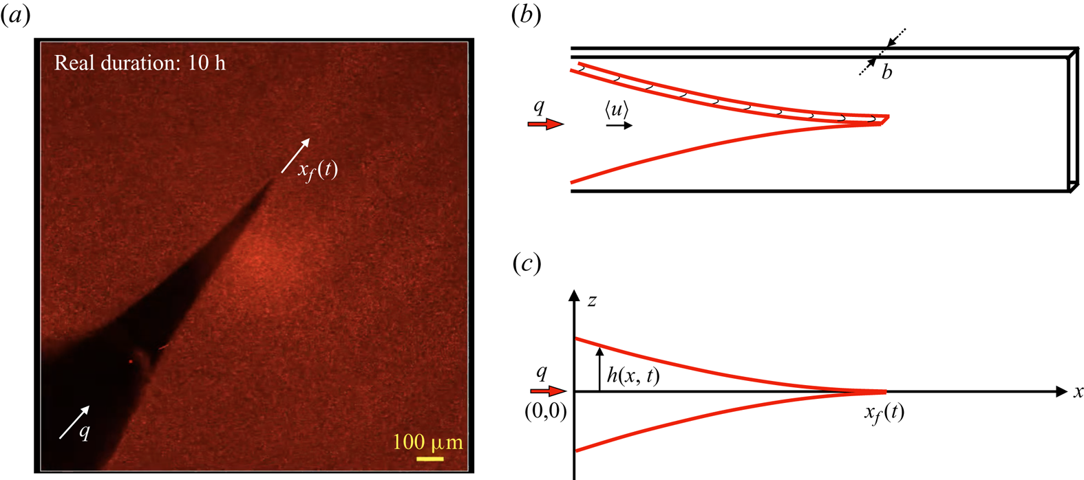
Figure 1. Hydraulic fracturing of an elastic solid in a Hele-Shaw cell. (a) A typical experimental picture of the tip region of a hydraulic fracture in a Hele-Shaw cell (e.g. Weitz Reference Weitz2020). (b) Schematic of the experimental picture. (c) Side view of a hydraulic fracture of the cusp shape near the tip.
This paper is structured as follows. We first present a theoretical model in § 2 based on the lubrication theory of viscous thin film flow within an elastically deformable cavity, which is coupled with the linear elastic theory of solid deformation for the distribution of the normal stress. This is analogous to previous models developed by e.g. Spence & Sharp (Reference Spence and Sharp1985), Spence et al. (Reference Spence, Sharp and Turcotte1987), Lister (Reference Lister1990a,Reference Listerb), Savitski & Detournay (Reference Savitski and Detournay2002), Detournay (Reference Detournay2004) and Roper & Lister (Reference Roper and Lister2007) to describe the growth of plane and radial fractures in an infinite elastic matrix without the influence of material toughness. Nevertheless, we arrive at a different nonlinear differential–integral system for the coupled evolution of fracture shape and pressure distribution, which leads to cusp shapes without pressure singularity. The theory also leads to self-similar solutions for both the fracture shape and pressure distribution at intermediate times. Then in § 3, we compare the theoretical predictions with available experimental observations from literature and time-dependent numerical solutions of the full nonlinear partial differential–integral system. We close the paper in § 4 with a brief summary and remarks on potential directions for future explorations.
2. Theoretical model
2.1. Governing equations
The model problem is sketched in figure 1, with a Newtonian liquid being injected into an elastic solid confined between two parallel plates of gap thickness  $b$. Neglecting the influence of body forces and interfacial tension, standard lubrication theory of viscous flow in a Hele-Shaw cell then indicates that the profile shape $h(x,t)$ of a fracture is governed by a partial differential equation
 \begin{equation} \frac{\partial h}{\partial t} - \frac{b^2}{12\mu}\,\frac{\partial}{\partial x} \left(h\,\frac{\partial p}{\partial x}\right) = 0, \end{equation}
with  $p(x,t)$ denoting the distribution of pressure within the liquid film that is to balance the normal stress of the elastically deformed solid at the fluid–solid interface. Equation (2.1) is different from (2.25) of Spence & Sharp (Reference Spence and Sharp1985), since the viscous drag within the liquid film is due predominantly to the no-slip boundary condition at the inner surface of the parallel plates rather than at the fluid–solid interface.
We constrain the model problem in the positive half-domain  $x \in [0,\infty ]$. The pressure distribution $p(x,t)$ within the liquid film due to elastic deformation is then given by
 \begin{equation} p(x,t)
={-}\frac{E}{2(1-\sigma^2)}\,\frac{1}{\rm \pi} \int_0^{x_f(t)}
\frac{1}{s-x}\,\frac{\partial h}{\partial s} \,{\rm d}s,
\end{equation}
\begin{equation} p(x,t)
={-}\frac{E}{2(1-\sigma^2)}\,\frac{1}{\rm \pi} \int_0^{x_f(t)}
\frac{1}{s-x}\,\frac{\partial h}{\partial s} \,{\rm d}s,
\end{equation}
where  $E$ is the Young's modulus of the elastic material, $\sigma$ is the Poisson ratio, and $x_f(t)$ is the location of the propagating front. The pressure distribution (2.2) due to elastic deformation is consistent with those in previous studies of plane and radial fractures in infinite elastic solids (e.g. Spence & Sharp Reference Spence and Sharp1985; Lister Reference Lister1990a,Reference Listerb). Since we focus only on the positive half-domain $x \in [0,\infty ]$, to be consistent with the experiment of e.g. Weitz (Reference Weitz2020), the lower limit of integration is $x = 0$ in (2.2) rather than $x = -x_f(t)$, which is the only difference from the well-cited literature (e.g. Spence & Sharp Reference Spence and Sharp1985; Lister Reference Lister1990a,Reference Listerb). The prefactor $1/{\rm \pi}$ is introduced from the definition of the Hilbert transform.
The differential–integral system (2.1) and (2.2) is to be solved providing appropriate initial and boundary conditions (IBCs), e.g. given by
 $$\begin{gather} h(x,0) = 0, \end{gather}$$
 $$\begin{gather}h(x_f(t),t) = 0, \end{gather}$$
 $$\begin{gather}\int_0^{x_f(t)}h(x,t)\,{\rm d}\kern0.7pt x = qt. \end{gather}$$
The initial condition (2.3a) indicates that there exists no fluid initially within the elastic solid, and fluid injection (i.e. fracturing) starts instantaneously at  $t=0$. The first boundary condition (2.3b) is a standard frontal condition (with compact support). The second boundary condition (2.3c) is a global constraint for the increase of total area within the plane of the paper, as covered by the fracturing fluid due to injection that proceeds at a constant rate $q$.
$q$.
The global volume conservation condition (2.3c) can also be shown to be equivalent to a flux condition at the injection point ( $x=0$):
 \begin{equation} \left.- \frac{b^2}{12\mu}\,h\,\frac{\partial p}{\partial x} \right|_{x=0} = q. \end{equation}
The treatment is similar to that for the propagation of a gravity current (e.g. Zheng et al. Reference Zheng, Guo, Christov, Celia and Stone2015). One can integrate the evolution equation (2.1) from  $x=0$ towards $x=x_f(t)$, imposing a zero-flux condition at the location of the propagating front $x=x_f(t)$ based on the assumption that there is no fluid loss or entrainment locally at $x=x_f(t)$. The integral constraint (2.3c) then reduces to a nonlinear flux condition (2.4). It is more convenient to solve the coupled evolution equations (2.1) and (2.2) numerically, subject to initial condition (2.3a), frontal condition (2.3b) and flux condition (2.4), e.g. with finite-volume schemes.
2.2. Scaling analysis
The form of the governing equations (2.1), (2.2) and IBCs (2.3) indicates the following scaling behaviours for the evolution of the length scale  $x$, thickness scale $h$, and pressure scale $p$:
$p$:
 $$\begin{gather} x \propto t^{1/2}
\left[\frac{b^2 E q}{24 {\rm \pi}(1-\sigma^2)
\mu}\right]^{1/4},
\end{gather}$$
$$\begin{gather} x \propto t^{1/2}
\left[\frac{b^2 E q}{24 {\rm \pi}(1-\sigma^2)
\mu}\right]^{1/4},
\end{gather}$$ $$\begin{gather}h \propto t^{1/2} \left[\frac{24 {\rm \pi}(1-\sigma^2) \mu q^3}{b^2 E}\right]^{1/4}, \end{gather}$$
 $$\begin{gather}p \propto \left[\frac{6 E \mu q}{{\rm \pi} (1-\sigma^2) b^2}\right]^{1/2}. \end{gather}$$
These scaling behaviours apply at intermediate times when  $x \gg b$ and $h \gg b$, such that the resistance for the elongation of a fracture comes predominantly from the viscous drag due to the no-slip condition at the surface of the parallel plates rather than at the fluid–solid interface. An estimate for the appropriate time scale is immediately available as $t \gg \max ([24{\rm \pi} (1-\sigma ^2)b^2 \mu /Eq]^{1/2}, [Eb^6/(24{\rm \pi} (1-\sigma ^2)\mu q^3)]^{1/2})$.
It is also seen that these scaling laws (2.5a–c) during hydraulic fracturing in a Hele-Shaw cell (e.g.  $x \propto t^{1/2}$ and $h \propto t^{1/2}$) are different from those (e.g. $x \propto t^{2/3}$ and $h \propto t^{1/3}$) for the growth of two-dimensional plane fractures of infinite depth (e.g. Spence & Sharp Reference Spence and Sharp1985). This is due to the difference of the velocity field of the lubricating flow and the viscous drag, which leads to a different scaling exponent of $h$ in the thin film equation (2.1).
2.3. Non-dimensionalisation
The scaling results also suggest the existence of self-similar solutions for the evolution of the fracture shape  $h(x,t)$ and pressure distribution $p(x,t)$. It is standard first to rescale the governing system (2.1) and (2.2) and the IBCs (2.3a–c). Since there exist no natural time or length scales within the plane of the fracture, we chose the gap thickness $b$ as a reference length scale, and define $h_c = b$. This would correspond to a time scale $t_c$ when the thickness of a fracture reaches $b$. Based on this choice, our model would work in the late-time regime $t \gg t_c$, when the length and thickness scales are both much greater than $b$. Accordingly, we define dimensionless variables as
 \begin{equation} \bar{t} \equiv \frac{t}{t_c}, \quad \bar{x} \equiv \frac{x}{x_c}, \quad \bar{h} \equiv \frac{h}{b}, \quad \bar{p}\equiv \frac{p}{p_c}, \end{equation}
where the characteristic time, length and pressure scales are chosen as
 \begin{align}
t_c = \left[\frac{b^6 E}{24
{\rm \pi} (1-\sigma^2) \mu q^3}\right]^{1/2}, \quad x_c =
\left[\frac{b^4 E}{24 {\rm \pi}(1-\sigma^2) \mu
q}\right]^{1/2},\quad p_c = \left[\frac{6 \mu q E }{{\rm \pi}
(1-\sigma^2) b^2}\right]^{1/2}.
\end{align}
\begin{align}
t_c = \left[\frac{b^6 E}{24
{\rm \pi} (1-\sigma^2) \mu q^3}\right]^{1/2}, \quad x_c =
\left[\frac{b^4 E}{24 {\rm \pi}(1-\sigma^2) \mu
q}\right]^{1/2},\quad p_c = \left[\frac{6 \mu q E }{{\rm \pi}
(1-\sigma^2) b^2}\right]^{1/2}.
\end{align} We then arrive at the dimensionless form of (2.1), (2.2) and IBCs (2.3), and for simplicity we continue to use  $t$,
$t$,  $x$,
$x$,  $h$ and $p$ to represent dimensionless variables in this section and § 3 from now on:
 $$\begin{gather} \frac{\partial h}{\partial t} = \frac{\partial}{\partial x} \left(h\,\frac{\partial p}{\partial x}\right), \end{gather}$$
 $$\begin{gather}p(x, t) ={-}\int_0^{x_f(t)} \frac{1}{s-x}\,\frac{\partial h}{\partial s} \,{\rm d}s, \end{gather}$$
and
 $$\begin{gather} h(x,0) = 0, \end{gather}$$
 $$\begin{gather}h(x_f(t), t) = 0, \end{gather}$$
 $$\begin{gather}\int_0^{x_f(t)} h(x, t)\,{\rm d}\kern0.7pt x = t. \end{gather}$$
Meanwhile, the dimensionless flux condition (2.4) is given by
 \begin{equation} \left.- h\,\frac{\partial p}{\partial x} \right|_{x=0} = 1, \end{equation}
which is equivalent to the integral constraint (2.9c). A finite-volume scheme is described in Appendix A that is employed to solve numerically the dimensionless system (2.8a,b) subject to (2.9a–c) for the coupled evolution of the dimensionless profile shape  $h(x, t)$ and pressure distribution $p(x, t)$.
Representative numerical solutions are shown in figure 2 for the time evolution of the profile shape  $h(x, t)$ and pressure distribution $p(x, t)$ for a hydraulic fracture within a Hele-Shaw cell. In particular, it is observed that the fracture develops into the cusp shape in a Hele-Shaw cell, which is consistent with the experimental observation in figure 1(a). This is also completely different from that of plane fractures of infinite depth with profiles in the form $h \propto (x_f - x)^{2/3}$ as $x \to x_f^-$. (In the viscous regime, see e.g. Spence & Sharp Reference Spence and Sharp1985.) The inset of figure 2(a) also shows that the normalised profile solutions collapse onto a universal shape, which suggests the existence of self-similarity, as we discuss later. Meanwhile, numerical solutions for the pressure distribution indicate that the pressure approaches a finite value as $x \to x_f^-$, which is also fundamentally different from the well-known pressure singularity of plane and radial fractures in the Cartesian and radial configurations (e.g. Spence & Sharp Reference Spence and Sharp1985; Spence et al. Reference Spence, Sharp and Turcotte1987; Lister Reference Lister1990a,Reference Listerb). Later, in § 3.1, these numerical solutions are also rescaled appropriately and compared with the self-similar solutions that we explore next.
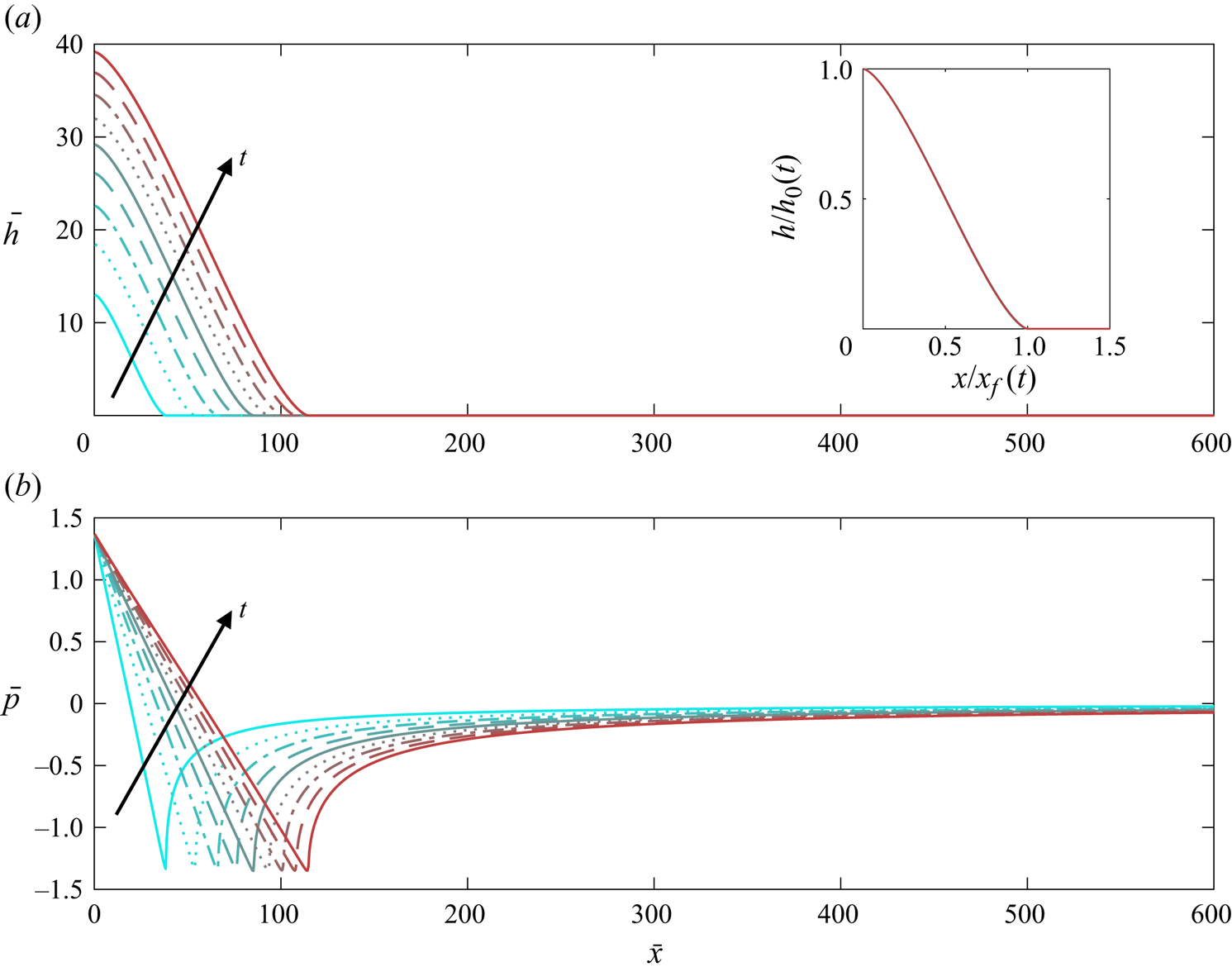
Figure 2. (a) Time evolution of cusp-like profile shapes  $h(x,t)$ near the front, and (b) time evolution of the pressure field $p(x, t)$, based on solving numerically the full partial differential–integral system (2.8a,b). The inset of (a) shows also that the normalised profiles collapse onto a universal shape. The profiles were taken at time $t = 250 \times \{1\unicode{x2013}9\}$. The domain length is $L=600$, with 1200 space grids employed here.
2.4. Self-similar solutions
To look for self-similar solutions of (2.8a,b) and (2.9a–c) at intermediate times ( $t \gg 1$), we start by defining a similarity variable as
 \begin{equation} \xi \equiv x/t^{1/2}. \end{equation}
We then look for  $h(x, t) = t^{1/2}\,k(\xi )$ and $p(x, t) = g(\xi )$ by solving
 $$\begin{gather} \frac{1}{2}\,k-\frac{1}{2}\,\xi\,\frac{{\rm d} k}{{\rm d} \xi} = \frac{{\rm d}}{{\rm d} \xi} \left(k\, \frac{{\rm d} g}{{\rm d} \xi}\right), \end{gather}$$
 $$\begin{gather}g(\xi) ={-} \int_0^{\xi_f} \frac{1}{s-\xi}\,\frac{{\rm d}k}{{\rm d} s} \,{\rm d}s, \end{gather}$$
subject to
 \begin{equation} k(\xi_f) = 0 \quad \mbox{and}\quad \int_0^{\xi_f} k(\xi)\,{\rm d}\xi = 1. \end{equation}
By definition,  $\xi _f \equiv x_f/t^{1/2}$ represents the frontal location. Meanwhile, the influence of initial condition (2.9a) no longer exists, as we are looking for intermediate time behaviours when $t \gg 1$.
To solve numerically the ordinary differential–integral system (2.12a,b) for the self-similar profile shape  $k(\xi )$ and pressure distribution $g(\xi )$, we keep the time dependence by introducing a mathematical transform
 \begin{equation} \tau = \ln t\quad \mbox{and}\quad \xi = x/t^{1/2}. \end{equation}
The original partial differential-integral system (2.8a,b) then becomes
 $$\begin{gather} -\frac{\partial k}{\partial \tau} + \frac{1}{2}\,k - \frac{1}{2}\,\xi\,\frac{\partial k}{\partial \xi} = \frac{\partial}{\partial \xi} \left(k\,\frac{\partial g}{\partial \xi}\right), \end{gather}$$
 $$\begin{gather}g ={-} \int_0^{\xi_f} \frac{1}{s-\xi}\,\frac{\partial k}{\partial s} \,{\rm d}s. \end{gather}$$
Compared with (2.12a,b), (2.15a,b) now include an additional term of time evolution  $\partial k/\partial \tau$. We then solve this evolution system for $k(\xi,\tau )$ and $g(\xi,\tau )$ using the same scheme as described in Appendix A, now subject to appropriate IBCs:
 $$\begin{gather} k(\xi,0) = 0, \end{gather}$$
 $$\begin{gather}k(\xi_f, \tau) = 0\quad \mbox{and}\quad \left. k\,\frac{\partial g}{\partial \xi} \right|_{\xi = 0} ={-}1. \end{gather}$$
This system is solved until there is negligible time evolution, as shown in figure 3, due to the existence of a sink term. The steady-state solutions  $k(\xi,\infty ) \to k_s(\xi )$ and $g(\xi,\infty ) \to g_s(\xi )$ become, effectively, the self-similar solutions of the ordinary differential–integral system (2.12a,b) that we are looking for. From figure 3, we also obtain the end-point values as $\xi _f \approx 2.42$, $k_s(0) \approx 0.82$, $g_s(0) \approx 1.37$ and $g_s(\xi _f) \approx -1.35$. For $g(\xi )$, relatively more significant numerical error appears around $\xi = \xi _f$, but this does not seem to influence the bulk structure. The stability of the self-similar solutions obtained here can also be studied based on the time-dependent system (2.15a,b) by adding small perturbations. Similar ideas have been employed before to study the development of finite-time singularities for thin fluid threads (e.g. Eggers & Fontelos Reference Eggers and Fontelos2009). To some extent, the transient dynamics here is similar to that of a propagating viscous gravity current that suffers also slow drainage from thin permeable substrates, driven by buoyancy or background flow (e.g. Pritchard, Woods & Hogg Reference Pritchard, Woods and Hogg2001). With fluid supply at a constant rate, the model problem evolves into steady flow solutions after an initial transition period, when fluid injection balances drainage.
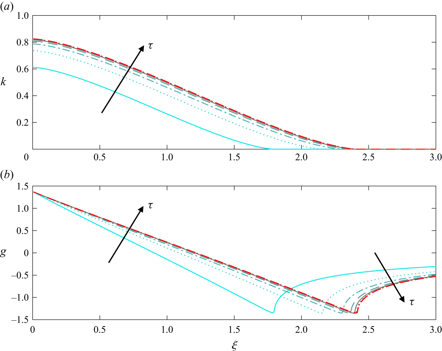
Figure 3. The partial differential–integral system (2.15a,b) is solved until there is negligible time evolution, i.e.  $k(\xi,\infty ) \to k_s(\xi )$, and $g(\xi,\infty ) \to g_s(\xi )$. The steady-state solutions are, effectively, the self-similar solutions of (2.12a,b). Here, the domain length is $L=3$ with 300 space grids employed, and we have included solutions at $\tau = 0.8\times \{1\unicode{x2013}8\}$.
It is of particular interest to note that the normalised solutions in figure 3 suggest that pressure decreases linearly towards the fracture's front while the profile shape develops into a cusp shape. It can also be shown that the following analytical solutions provide very good predictions:
 $$\begin{gather} h/h_0 ={-}{\rm \pi}^{{-}1}\left[(2\eta - 1)[1-(2\eta-1)^2]^{1/2} + \sin^{{-}1}(2\eta-1) - {\rm \pi}/2\right], \end{gather}$$
 $$\begin{gather}p/p_0 = (1 - 2\eta), \end{gather}$$
where  $\eta \equiv \xi /\xi _f = x/x_f \in [0,1]$, as we included also in figure 3 as well. In particular, (2.17a) indicates that
 \begin{equation} h/h_0 \propto (1-x/x_f)^{3/2}, \end{equation}
as  $x \to x_f(t)^-$, which describes the cusp shape. More discussions on the frontal structure (2.17a,b) and the universal behaviours of the profile shape and pressure distribution are provided in Appendix B based on series expansions.
3. Numerical and experimental observations
In this section, we first provide a detailed comparison between the self-similar solutions and the time-dependent numerical solutions of the full partial differential–integral system (2.8a,b). We then provide brief remarks on some experimental observations taken from the literature.
3.1. Comparison with time-dependent numerical solutions
We first provide a comparison between the self-similar solution and the time-dependent numerical solutions of the partial differential–integral system (2.8a,b). In particular, the time-dependent numerical solutions for the evolution of the profile shape and pressure distribution in figure 2 are now rescaled appropriately based on the maximum values in figure 4, which exhibits very good collapse onto universal curves. We then include in the same figure the (appropriately stretched) self-similar solutions from solving numerically (2.15a,b), which provides very good agreement with the collapsed numerical solutions.
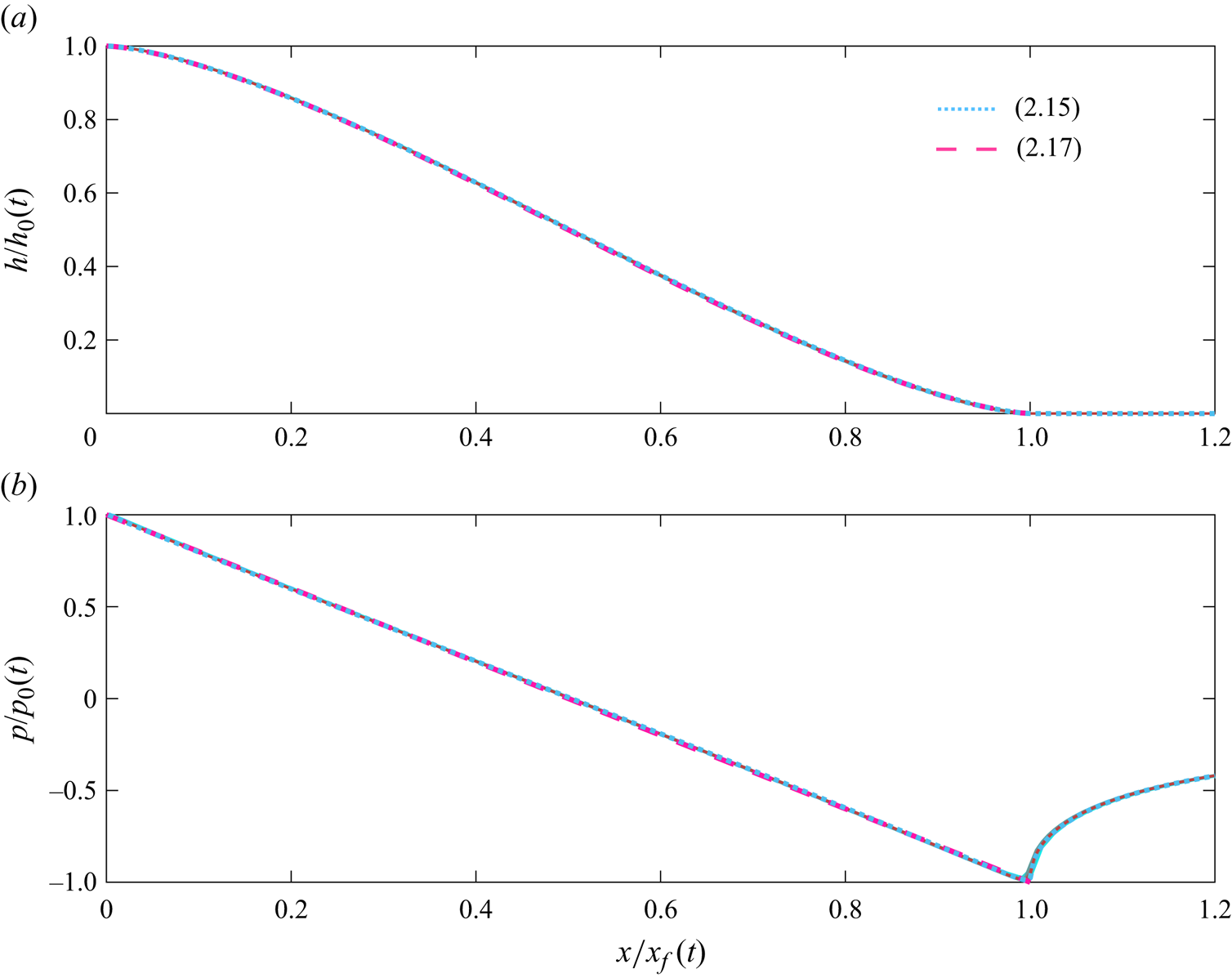
Figure 4. The rescaled solutions of the profile shape and pressure field evolution of the numerical data in figure 2. They already collapse onto universal curves, which also exhibits reasonably good agreement with the prediction of the self-similar solutions from solving (2.15a,b) until there is negligible time evolution, shown as the dashed curves.
Meanwhile, we track the time-dependent frontal location  $x_f(t)$, inlet thickness $h_0(t) \equiv h(0, t)$, inlet pressure $p_0(t) = p(0, t)$ and tip pressure $p_f(t) \equiv p(x_f(t), t)$ from numerical solutions of (2.8a,b). In all cases, the numerical solutions (the symbols) approach the prediction of the self-similar solutions from solving numerically (2.15a,b) at intermediate times, shown as the solid lines in figure 5, and as described by
 \begin{equation} x_f(t) \sim 2.42\, t^{1/2},\quad h_0(t) \sim 0.82\, t^{1/2},\quad p_0(t) \sim 1.37\quad \mbox{and}\quad p_f(t) \sim{-}1.35. \end{equation}
There is very good agreement for both the scaling exponents of time dependence and the prefactors between the self-similar and numerical solutions. The very small difference, we believe, is more likely due to numerical error (e.g. on the last digit of solution (3.1a–d)) and is less likely due to unfinished time transition.
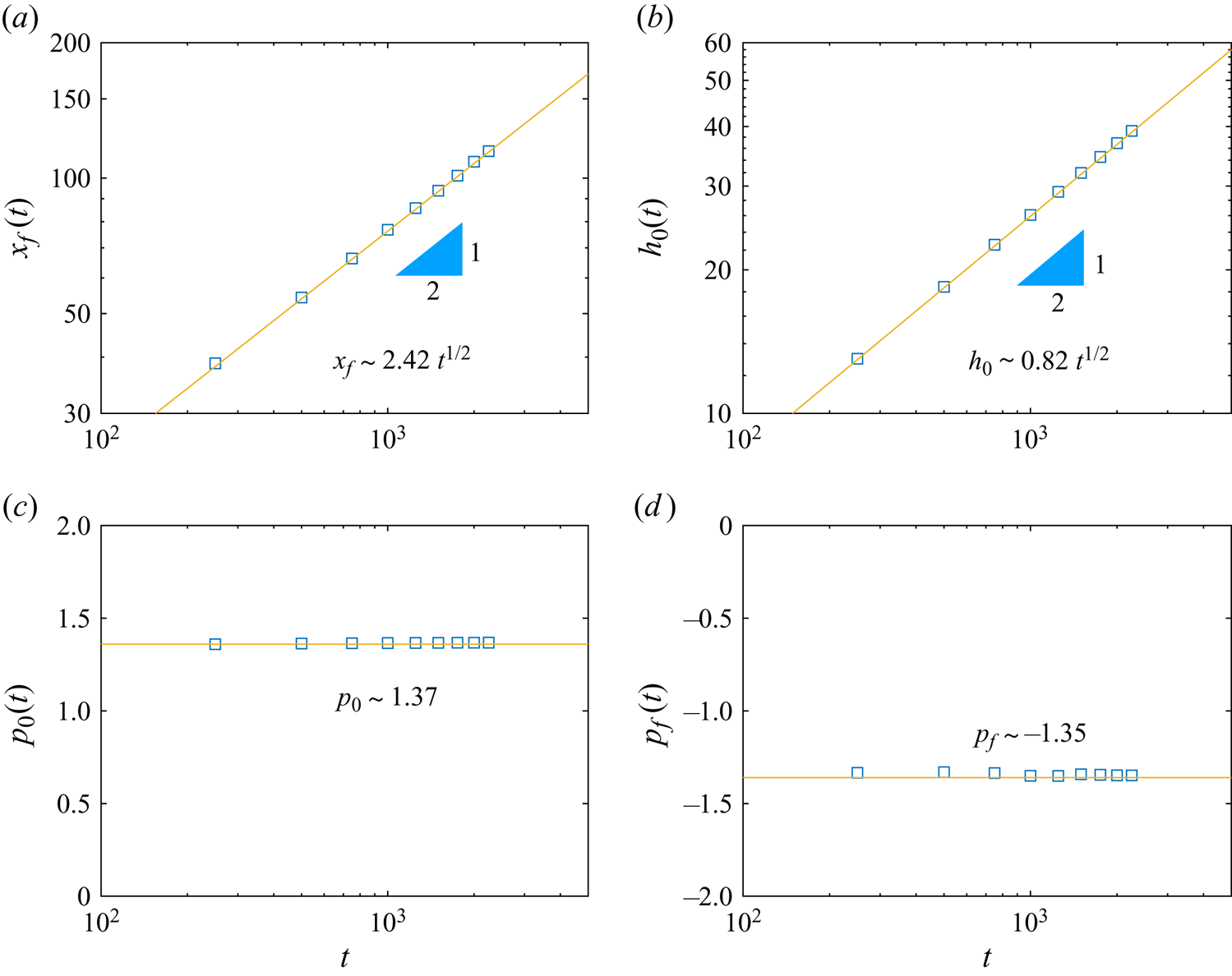
Figure 5. Time evolution of the frontal location  $x_f(t)$, fracture thickness $h_0(t) \equiv h(0,t)$, inlet pressure $p_0(t) \equiv p(0, t)$, and tip pressure $p_f(t) \equiv p(x_f(t), t)$, based on solving numerically the partial differential–integral system (2.8a,b). The numerical results (symbols) agree very well with the prediction of the self-similar solutions (solid lines) at intermediate times.
3.2. Comparison with available experimental observations
There are also limited experimental pictures available from the literature (e.g. Weitz Reference Weitz2020; Aime et al. Reference Aime, Sabato, Xiao and Weitz2021). In a typical experiment, a fluid such as air or water is injected through a syringe pump into a thin layer of colloidal gel that is confined between the two parallel plates of a Hele-Shaw cell, as shown in figure 6. The porosity of the gel (1.875 % Ludox Gel, SM 40) is  $\approx$70 %, the modulus is ${\approx }100$ kPa, and the yield stress is $\approx$480 Pa from measurements. The Hele-Shaw cell has length 7.5 cm, width 5.0 cm, and thickness $7\ \mathrm {\mu }{\rm m}$. The injection rate is small, and typical propagating speed of a hydraulic fracture is ${\approx }1\ \mathrm {\mu }{\rm m}\ {\rm s}^{-1}$. A typical experiment lasts for 1–10 h.
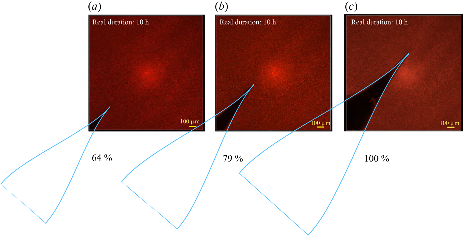
Figure 6. Experimental pictures at three different times for the profile shape of a hydraulic fracture in a Hele-Shaw cell (e.g. Weitz Reference Weitz2020), while the appropriately stretched theoretical predictions from solving (2.8a,b) are superimposed as the cyan curves.
A comparison between experimentally recorded (e.g. Weitz Reference Weitz2020) and rescaled (and collapsed) numerical solutions of the full partial differential–integral system (2.8a,b) is shown in figure 6 for the profile shape of a hydraulic fracture in a Hele-Shaw cell. Experimental pictures of the near-tip region of the profile shape at three different times are shown in figures 6(a–c), respectively, with the appropriately stretched numerical solutions superimposed on each of them. In particular, the length scales at two different times  $t_1$ and $t_2$ must satisfy $x_1/x_2 = h_1/h_2 = (t_1/t_2)^{1/2}$ at the self-similar stage based on the scaling laws (2.5a,b). We observe fairly good agreement between the theoretical and experimental results of this cusp-shaped hydraulic fracture in a Hele-Shaw cell. We do recognise that the available experimental data are rather limited. So we suggest further experiments being performed in the future with time-dependent profile shapes and possibly pressure fields reported, which would allow more thorough comparison with the theory.
4. Summary and final remarks
4.1. Summary
A theoretical model is provided to describe the coupled evolution of the profile shape and pressure distribution of a hydraulic fracture in a Hele-Shaw cell. The model is based on the lubrication theory of viscous thin film flow in an elastically deformable cavity, which is coupled with the linear elastic theory of solid deformation for the distribution of normal stresses at the fluid–solid interface (i.e. the distribution of pressure within the liquid film). It is of particular interest to note that the model leads to hydraulic fractures of cusp shapes, which is consistent with recent experimental observations in a Hele-Shaw cell. The model also suggests the existence of self-similar solutions at intermediate times, which is verified through a comparison with rescaled numerical solutions of the full partial differential–integral system (2.8a,b). Compared with the classic results of plane or penny-shaped fractures, there exists no pressure singularity at the tip of a hydraulic fracture in a Hele-Shaw cell, which is a fundamental difference. We suggest that more experiments should be performed in the future to obtain time-dependent data of the fracture shape, frontal location, and pressure distribution (if possible), which can be used to further verify the theory and/or suggest new directions for future explorations.
4.2. Time-dependent injection modes
The theoretical model works also when the injection rate is time-dependent, as already pointed out in earlier studies on the propagation of plane and radial hydraulic fractures in elastic solids (e.g. Spence & Sharp Reference Spence and Sharp1985; Lai et al. Reference Lai, Zheng, Dressaire, Wexler and Stone2015). This is also true for the growth of a hydraulic fracture in a Hele-Shaw cell in the current work. Of particular interest is the situation when the injection rate follows power-law or exponential forms of time dependence, in which case self-similar solutions can also be explored to describe the universal behaviours at intermediate times. Here, we briefly point out that under a power-law form of fluid injection, such that the total volume (area) follows  $V(t) = q t^\alpha$, the scaling results (2.5a–c) are extended to
 $$\begin{gather} x \propto
t^{(\alpha+1)/4} \left[\frac{b^2 Eq}{24 {\rm \pi}(1-\sigma^2)
\mu}\right]^{1/4},
\end{gather}$$
$$\begin{gather} x \propto
t^{(\alpha+1)/4} \left[\frac{b^2 Eq}{24 {\rm \pi}(1-\sigma^2)
\mu}\right]^{1/4},
\end{gather}$$ $$\begin{gather}h \propto t^{(3\alpha-1)/4} \left[\frac{24 {\rm \pi}(1-\sigma^2) \mu q^3}{b^2 E}\right]^{1/4}, \end{gather}$$
 $$\begin{gather}p \propto t^{(\alpha-1)/2} \left[\frac{6 \mu q E }{{\rm \pi} (1-\sigma^2) b^2}\right]^{1/2}, \end{gather}$$
to describe the time evolution of the length and pressure scales. We stop the discussion here by noting simply that self-similar solutions for the profile shape  $h(x,t)$ and pressure distribution $p(x,t)$ can also be explored following the procedure in § 2.4 of the current work.
4.3. The influence of material toughness
It is well known that the propagation of a hydraulic fracture can possibly be resisted by material breaking at the fracture tip as well. In the well-cited literature of hydraulic fracturing of an infinite elastic solid that is also brittle (e.g. Spence & Sharp Reference Spence and Sharp1985; Lister Reference Lister1990b; Savitski & Detournay Reference Savitski and Detournay2002; Roper & Lister Reference Roper and Lister2007), a revised model is to introduce a propagation condition
 \begin{equation} K_{c} \sim \frac{E}{2^{3/2}(1-\sigma^2)}\,\frac{h(x,t)}{(x_f(t)-x)^{1/2}}, \end{equation}
as  $x \to x_f(t)^-$. Condition (4.2) is consistent with those derived based on the theory of linear elastic fracture mechanics of a mode I crack without the influence of body forces and that of flow (e.g. Rice Reference Rice1968; Howell, Kozyreff & Ockendon Reference Howell, Kozyreff and Ockendon2008). The critical stress intensity factor $K_{c} > 0$ is typically named ‘material toughness’ and is an important property of a brittle material. Detailed analysis of the influence of material breaking on hydraulic fracturing in a Hele-Shaw cell is left for a future work. In such a context, the description of (2.1a,b) subject to IBCs (2.3) applies, when fracturing a non-brittle elastic material as $K_{c} \to 0^+$.
Acknowledgements
We would like to thank C.-Y. Lai, P.F. Linden, N.J. O'Keeffe, and H.A. Stone for many insightful discussions on hydraulic fracturing. We also thank the reviewers of this work for helpful comments.
Funding
Partial support is acknowledged from a QJMAM award (no. 1017777) and NSFC (no. 12272235). This work was also partially supported by the Program for Professor of Special Appointment (Eastern Scholar, no. TP2020009) at Shanghai Institutions of Higher Learning.
Declaration of interests
The authors report no conflict of interest.
Appendix A. Numerical scheme
A finite-volume scheme is developed to solve numerically the governing nonlinear non-local system (2.8a,b) for the coupled profile shape and pressure evolution of a hydraulic fracture. For simplicity, we use  $x$,
$x$,  $t$,
$t$,  $h$ and $p$ to denote the dimensionless variables here. To start, we chose the cell-centred discretisation method for a finite-volume scheme. The domain of length $L$ is first discretised as $x_n = (n-1/2)\,\Delta x$ for $n=1,2,\ldots,N$, where the space step is $\Delta x = L/(N-1)$. Time is also discretised as $t_i = i\,\Delta t$ for $i = 0,1,2,\ldots$, and the time step is chosen as $\Delta t = c (\Delta x)^3$ for a third-order scheme (in space). The constant $c$ is small enough to ensure that the scheme is stable.
The evolution system (2.8a) is then rewritten as
 \begin{equation} h_n^{i+1} = h_n^i + \frac{\Delta t}{\Delta x}\left(q_{n+1/2}^i-q_{n-1/2}^i\right), \end{equation}
for  $n=1,2,\ldots,N$. Meanwhile, the dimensionless flux $q_{n+1/2}^i$ (or $q_{n-1/2}^i$) is defined at the boundary of two neighbouring grids as
 \begin{equation} q_{n-1/2}^i = \frac{h_{n}^i + h_{n-1}^i}{2}\,\frac{p_{n}^i - p_{n-1}^i}{\Delta x}, \end{equation}
with  $n = 2,\ldots,N$, and the dimensionless pressure $p_n^i$ is given by the discretised version of the integral equation (2.8b) as
 \begin{equation} p_n^i ={-} \sum_1^{n_f-1} \frac{h_{k+1}^i-h_k^i}{(x_{k+1}+x_k)/2-x_n}, \end{equation}
with  $n_f$ denoting the location of the propagating front (the crack tip), which locates at $x_f = (n_f - 1/2)\,\Delta x$. For such a finite-volume scheme, the flux boundary conditions are convenient to impose as
 \begin{equation} q_{1/2}^i = 1\quad\mbox{and}\quad q_{N-1/2}^i = 0. \end{equation}
Then we can obtain numerical solutions for the profile shape  $h_n^i$ and pressure distribution $p_n^i$ for $i=1,2,3,\ldots$ and $n=1,2,\ldots,N$, providing the initial conditions such as $h_n^0 = 0$ and $p_n^0 = 0$ for $n = 1,2,\ldots,N$.
The scheme is second order in space except at the boundary points, where it is first order, and first order (explicit) in time. The space and time steps are chosen to be small enough such that the scheme is stable, and no significant difference appears subject to further grid refinement. Volume conservation is also checked as time progresses. A typical grid number is  $N = {O}(10^3)$, and the constant chosen is $c = {O}(10^{-3})$. Similar schemes have been employed before to obtain numerical solutions for nonlinear differential systems of gravity current flows in confined porous layers (e.g. Zheng et al. Reference Zheng, Guo, Christov, Celia and Stone2015; Hinton & Woods Reference Hinton and Woods2018) and capillary-driven thin film flows (e.g. Zheng et al. Reference Zheng, Fontelos, Shin, Dallaston, Tseluiko, Kalliadasis and Stone2018). This scheme has also been modified appropriately to deal with the plane fracture problem without material toughness (see e.g. Spence & Sharp Reference Spence and Sharp1985). We found that it is able to capture the universal fracture shape $h \propto (x_f-x)^{2/3}$ as $x \to x_f^-$. It is also able to demonstrate clearly the development of a logarithm singularity for pressure distribution near the fracture tip, with (local) numerical error as $x \to x_f^-$ depending significantly on the grid number, as expected.
Appendix B. Frontal structures
We start by noting that the ordinary differential–integral system (2.12a,b) can be stretched appropriately by further defining  $\eta \equiv \xi /\xi _f \in [0,1]$ such that the frontal location is $\eta _f = 1$ in the $(\eta, k)$ space. For correct balance, we also define $\mathcal {K}(\eta ) \equiv k(\xi )/\xi _f^3$ and $\mathcal {G}(\eta ) \equiv g(\xi )/\xi _f^2$, and (2.12) and (2.13{a,b}) now become
 $$\begin{gather} \frac{1}{2}\,\mathcal{K}-\frac{1}{2}\,\eta\,\frac{{\rm d} \mathcal{K}}{{\rm d} \eta} = \frac{{\rm d}}{{\rm d} \eta} \left(\mathcal{K}\,\frac{{\rm d} \mathcal{G}}{{\rm d} \eta}\right), \end{gather}$$
 $$\begin{gather}\mathcal{G}(\eta) ={-} \int_0^{1} \frac{1}{s-\eta}\,\frac{{\rm d}\mathcal{K}}{{\rm d} s}\,{\rm d}s, \end{gather}$$
and
 \begin{equation} \mathcal{K}(1) = 0 \quad \mbox{and}\quad \xi_f = \left[\int_0^{1} \mathcal{K}(\eta)\,{\rm d}\eta\right]^{{-}1/4}. \end{equation}
It is more convenient to look for asymptotic solutions for (B1a,b) on  $\eta \in [0,1]$, compared with looking for solutions for (2.12a,b) on $\xi \in [0,\xi _f]$ since $\xi _f$ is unknown.
If we further make the transform  $\eta \equiv (r+1)/2 \in [0,1]$ such that the domain of the integral equation (B1b) for elasticity becomes $r \in [-1,1]$, to be consistent with the earlier works of plane fractures in infinite elastic solids (e.g. Spence & Sharp Reference Spence and Sharp1985), for a linearly decreasing normalised pressure profile $\mathcal {G}_m^{-1}\mathcal {G}(r) = -r$ (i.e. $\mathcal {G}_m^{-1}\mathcal {G}(\eta ) = 1-2\eta$) that is consistent with the numerical observations in figure 3, standard identities of the Hilbert transform then indicate that $\mathcal {K}_m^{-1}\,{\rm d}\mathcal {K}/{\rm d}r = -{\rm \pi} ^{-1} (1-r^2)^{1/2}$, as pointed out by a reviewer of this work. Here, $\mathcal {G}_m$ and $\mathcal {K}_m$ represent the end-point maximum values for the profile shape and fluid pressure at $r=-1$ (i.e. $\eta =0$). We can then integrate this solution once to provide $\mathcal {K}_m^{-1}\mathcal {K}(r) = {\rm \pi}^{-1}[r(1-r^2)^{1/2} + \sin ^{-1}r - {\rm \pi}/2]$, which satisfies also the frontal condition $\mathcal {K}(1) = 0$. Equivalently, these solutions become (see (2.17a,b))
 $$\begin{gather} \mathcal{K}_m^{{-}1}\mathcal{K}(\eta) ={-}{\rm \pi}^{{-}1}\left[(2\eta - 1)[1-(2\eta-1)^2]^{1/2} + \sin^{{-}1}(2\eta-1) - {\rm \pi}/2\right], \end{gather}$$
 $$\begin{gather}\mathcal{G}_m^{{-}1}\mathcal{G}(\eta) = (1 - 2\eta), \end{gather}$$
for  $\eta \in [0,1]$. Solutions (B3a,b) are found to provide very good agreement with the normalised self-similar solutions and the rescaled time-dependent numerical solutions throughout the entire domain, as shown also in figure 3. Solution (B3a) can also be expanded around the fracture's tip to provide
 \begin{equation} \mathcal{K}_m^{{-}1}\mathcal{K}(\eta) \propto (1-\eta)^{3/2}, \end{equation}
as  $\eta \to 1^-$, which is solution (2.18) for the fracture's cusp-shaped profile near the tip.
In fact, we can show that solutions (B3a,b) are also compatible with the flow equation (B1a). We start by imposing series solutions of the power-law form for  $\mathcal {K}(\eta )$ and $\mathcal {G}(\eta )$ as
 $$\begin{gather} \mathcal{K}(\eta) = \sum A_i(1-\eta)^{\alpha+i-1}, \end{gather}$$
 $$\begin{gather}\mathcal{G}(\eta) = B_0 + \sum B_i(1-\eta)^{\beta+i-1}, \end{gather}$$
where  $\alpha > 0$, $\beta > 0$, and $i=1,2,\ldots,I$. By substituting (B5a,b) into the flow equation (B1a), appropriate balance at different orders of $(1-\eta )^{\alpha }$ leads to $\beta = 1$, which is independent on the value of $\alpha$ for the profile shape, and
 $$\begin{gather} B_1 = 1/2,\quad\mbox{at}\ {O}\left[(1-\eta)^{\alpha-1}\right], \end{gather}$$
 $$\begin{gather}B_2 = 1/4(\alpha+1),\quad\mbox{at}\ {O}\left[(1-\eta)^{\alpha}\right], \end{gather}$$
as  $\eta \to 1^-$. We can include more higher-order terms here. It is already shown, nevertheless, that the pressure distribution must be linear at leading order, which is consistent with solution (B3b) and the numerical solutions in figure 3. The value of $\alpha$ is undetermined as of now. However, if we impose $\alpha =3/2$ based on (B4), then by substituting the leading-order profile shape $\mathcal {K}(\eta ) \sim A_1(1-\eta )^{3/2}$ back into the elasticity equation (B1b), we obtain
 \begin{align} \mathcal{G}(\eta)& = B_0+3A_1 \left[1-(1-\eta)^{1/2}\, \mbox{tanh}^{{-}1} (1-\eta)^{{-}1/2}\right] \nonumber\\ &\sim (B_0+3A_1) - 3A_1(1-\eta) + {O}\left[(1-\eta)^{2}\right], \end{align}
as  $\eta \to 1^-$. At leading order, this provides also a linear pressure distribution from the elasticity equation. Therefore, solutions (B3a,b) are compatible with both the flow and elasticity equations. It might be of interest to note that the fractional-power expansions for the profile shape (B5a) are consistent with previous studies on edge cracks without flow (from solving a biharmonic equation for stress) (e.g. Williams Reference Williams1957).


