


1. Introduction
Strong acoustic tones are generated when a high subsonic jet or a supersonic jet impinge on a plate (Neuwerth Reference Neuwerth1974; Ho & Nosseir Reference Ho and Nosseir1981; Powell Reference Powell1988; Jaunet et al. Reference Jaunet, Mancinelli, Jordan, Towne, Edgington-Mitchell, Lehnasch and Girard2019). Numerous studies have shown that these tones are due to the establishment of aeroacoustic feedback loops between the jet nozzle and the plate. These feedback loops involve downstream- and upstream-propagating waves described in the recent review by Edgington-Mitchell (Reference Edgington-Mitchell2019). The downstream part consists of large-scale coherent structures resulting from the amplification and saturation of Kelvin–Helmholtz instability waves in the jet mixing layers. As these large-scale structures interact with the plate or with a standoff shock that may form near the plate, they generate waves that propagate up to the jet nozzle and excite new instability waves in the near-nozzle mixing layers, thus completing the feedback loop. While the upstream part of the feedback loops was initially assumed to be free-stream sound waves (Ho & Nosseir Reference Ho and Nosseir1981; Powell Reference Powell1988), Tam & Ahuja (Reference Tam and Ahuja1990) and, afterwards, many authors (Tam & Norum Reference Tam and Norum1992; Panickar & Raman Reference Panickar and Raman2007; Gojon, Bogey & Marsden Reference Gojon, Bogey and Marsden2016; Bogey & Gojon Reference Bogey and Gojon2017; Jaunet et al. Reference Jaunet, Mancinelli, Jordan, Towne, Edgington-Mitchell, Lehnasch and Girard2019; Ferreira et al. Reference Ferreira, Fiore, Parisot-Dupuis and Gojon2023; Varé & Bogey Reference Varé and Bogey2023), showed that the feedback loops are closed, in most cases, by intrinsic modes of the jets, called guided jet modes in recent papers. These modes were first studied in detail by Tam & Hu (Reference Tam and Hu1989) using linear stability analyses (LSA) and by modelling jets as vortex sheets of infinite length. As for duct modes, they are classified depending on their azimuthal and radial structures, and satisfy specific dispersion relations (Towne et al. Reference Towne, Cavalieri, Jordan, Colonius, Schmidt, Jaunet and Brès2017; Bogey Reference Bogey2021). Some of the guided jet waves (GJWs), called free-stream GJWs (Towne et al. Reference Towne, Cavalieri, Jordan, Colonius, Schmidt, Jaunet and Brès2017; Bogey Reference Bogey2021, Reference Bogey2022a), propagate upstream at a velocity close to the speed of sound and have significant amplitudes outside the jet column. They are allowed only in narrow frequency bands, in which the tone frequencies obtained in the upstream direction of high subsonic free jets (Schmidt et al. Reference Schmidt, Towne, Colonius, Cavalieri, Jordan and Brès2017; Towne et al. Reference Towne, Cavalieri, Jordan, Colonius, Schmidt, Jaunet and Brès2017; Bogey Reference Bogey2021, Reference Bogey2022b; Zaman, Fagan & Upadhyay Reference Zaman, Fagan and Upadhyay2022, Reference Zaman, Fagan and Upadhyay2023), in screeching jets (Shen & Tam Reference Shen and Tam2002; Edgington-Mitchell et al. Reference Edgington-Mitchell, Jaunet, Jordan, Towne, Soria and Honnery2018, Reference Edgington-Mitchell, Li, Liu, He, Wong, Mackenzie and Nogueira2022; Gojon, Bogey & Mihaescu Reference Gojon, Bogey and Mihaescu2018; Mancinelli et al. Reference Mancinelli, Jaunet, Jordan and Towne2019; Nogueira et al. Reference Nogueira, Jaunet, Mancinelli, Jordan and Edgington-Mitchell2022), in jets grazing a plate (Jordan et al. Reference Jordan, Jaunet, Towne, Cavalieri, Colonius, Schmidt and Agarwal2018; Tam & Chandramouli Reference Tam and Chandramouli2020) and in impinging jets (Tam & Norum Reference Tam and Norum1992; Panickar & Raman Reference Panickar and Raman2007; Gojon et al. Reference Gojon, Bogey and Marsden2016; Bogey & Gojon Reference Bogey and Gojon2017; Jaunet et al. Reference Jaunet, Mancinelli, Jordan, Towne, Edgington-Mitchell, Lehnasch and Girard2019; Ferreira et al. Reference Ferreira, Fiore, Parisot-Dupuis and Gojon2023; Varé & Bogey Reference Varé and Bogey2023) fall in most cases.
For impinging jets, the effects of the Mach number and of the nozzle-to-plate distance on the tone frequencies have been documented in several studies (Ho & Nosseir Reference Ho and Nosseir1981; Powell Reference Powell1988; Panickar & Raman Reference Panickar and Raman2007; Gojon et al. Reference Gojon, Bogey and Marsden2016; Gojon & Bogey Reference Gojon and Bogey2017a; Jaunet et al. Reference Jaunet, Mancinelli, Jordan, Towne, Edgington-Mitchell, Lehnasch and Girard2019; Varé & Bogey Reference Varé and Bogey2023). For Mach numbers lower than  $0.65$, no tones have been measured (Marsh Reference Marsh1961; Preisser Reference Preisser1979; Neuwerth Reference Neuwerth1974), whereas tones usually emerge for higher Mach numbers (Jaunet et al. Reference Jaunet, Mancinelli, Jordan, Towne, Edgington-Mitchell, Lehnasch and Girard2019; Varé & Bogey Reference Varé and Bogey2023). For a given Mach number, the tone frequencies decrease as the nozzle-to-plate distance increases (Neuwerth Reference Neuwerth1974; Ho & Nosseir Reference Ho and Nosseir1981; Powell Reference Powell1988; Panickar & Raman Reference Panickar and Raman2007), but suddenly rise discontinuously for certain distances, exhibiting a mode staging phenomenon typical of those observed in resonant flows. For a given nozzle-to-plate distance, the tone frequencies overall decrease as the Mach number increases and mode staging phenomena also occur (Jaunet et al. Reference Jaunet, Mancinelli, Jordan, Towne, Edgington-Mitchell, Lehnasch and Girard2019; Varé & Bogey Reference Varé and Bogey2023). For Mach numbers between $0.7$ and $0.95$, Tam & Ahuja (Reference Tam and Ahuja1990) showed that the average tone frequency, determined by averaging the tone frequencies obtained for different nozzle-to-plate distances, agree with the lowest frequency of the least-dispersed GJW. However, for Mach numbers lower than $0.65$, the lowest Strouhal number of the least-dispersed GJW is higher than ${St}=f\kern0.7pt D/u_j=0.85$ (Bogey Reference Bogey2021), where $f$ is the frequency, $D$ is the nozzle diameter, and $u_j$ is the jet velocity. Therefore, it is unlikely to fall within the Strouhal number range of the instability waves significantly amplified between the nozzle and the plate, typically $0.3\lesssim {St} \lesssim 0.7$ for jets with turbulent exit boundary layers (Tam & Ahuja Reference Tam and Ahuja1990; Varé & Bogey Reference Varé and Bogey2023), which may explain the absence of tones for Mach numbers lower than $0.65$ (Tam & Ahuja Reference Tam and Ahuja1990).
In the different experiments of the literature on impinging jets, the tone frequencies for a given nozzle-to-plate distance differ in some cases. For example, for jets at Mach number  $0.8$ impinging on a plate located at four nozzle diameters from the nozzle, Jaunet et al. (Reference Jaunet, Mancinelli, Jordan, Towne, Edgington-Mitchell, Lehnasch and Girard2019) reported a tone at Strouhal number ${St}=0.34$, while Panickar & Raman (Reference Panickar and Raman2007) measured a tone at ${St}=0.52$. Discrepancies can also be observed between the tone frequencies obtained in high-fidelity numerical simulations and in experiments. This is the case, for instance, between the tone frequencies in the numerical study of Varé & Bogey (Reference Varé and Bogey2023) and those measured by Jaunet et al. (Reference Jaunet, Mancinelli, Jordan, Towne, Edgington-Mitchell, Lehnasch and Girard2019) for jets at Mach numbers lower than $0.9$. The discrepancies are often attributed to differences in the nozzle-exit conditions, boundary-layer thickness and initial turbulence levels, which are not always known in the experiments. Indeed, the influence of the nozzle-exit conditions on the flow and noise of free jets has been shown to be significant in numerous studies (Zaman Reference Zaman1985a, Reference Zaman2012; Bridges & Hussain Reference Bridges and Hussain1987; Viswanathan & Clark Reference Viswanathan and Clark2004; Kim & Choi Reference Kim and Choi2009; Bogey & Bailly Reference Bogey and Bailly2010; Bogey, Marsden & Bailly Reference Bogey, Marsden and Bailly2012; Bogey & Marsden Reference Bogey and Marsden2013; Fontaine et al. Reference Fontaine, Elliott, Austin and Freund2015; Brès et al. Reference Brès, Jordan, Jaunet, Le Rallic, Cavalieri, Towne, Lele, Colonius and Schmidt2018; Bogey & Sabatini Reference Bogey and Sabatini2019). For laminar boundary layers, the mixing layers are characterized by the formation of vortices resulting from the growth of Kelvin–Helmholtz instability waves. As they are convected in the downstream direction, the vortices interact with each other and merge, generating pairing noise. For thicker boundary layers, the growth rates of the most amplified instability waves near the nozzle are lower, leading to a shear-layer rolling-up occurring later, and to a thinner mixing layer approximately between one and four nozzle radii from the nozzle exit (Kim & Choi Reference Kim and Choi2009; Bogey & Bailly Reference Bogey and Bailly2010).
The effects of the nozzle-exit conditions can also be expected to be significant in impinging jets. Since the properties of the Kelvin–Helmholtz instability waves vary with the nozzle-exit conditions in free jets (Michalke Reference Michalke1984; Bogey & Bailly Reference Bogey and Bailly2010; Morris Reference Morris2010; Bogey & Sabatini Reference Bogey and Sabatini2019), the gain in amplitude of the instability waves between the nozzle and the plate, and consequently, the strength of the resonance phenomena, should also vary. For thicker laminar boundary layers, in particular, the nozzle-to-plate gain in amplitude of the instability waves at high Strouhal numbers may be counter-intuitively stronger because of the slower mixing-layer development mentioned above. For Mach numbers lower than  $0.65$, this could enable the establishment of feedback loops at the Strouhal number of the least-dispersed GJW. Very recently, Varé & Bogey (Reference Varé and Bogey2024) examined the effects of the nozzle-exit fluctuation levels on the tones generated by impinging jets for Mach numbers between $0.6$ and $1.3$. Overall, they reported weaker tones and tone frequencies in better agreement with the experiments of the literature for initially laminar jets than for initially disturbed ones.
Given the above, the influence of the boundary-layer thickness on the noise generated by subsonic impinging round jets is investigated in the present study using large-eddy simulations (LES). Three jets at Mach number  $0.9$ and three jets at Mach number $0.6$, with boundary-layer thicknesses ranging from $0.05 r_0$ to $0.2 r_0$, where $r_0=D/2$, are considered. All the jets impinge on a flat plate located at $6$ nozzle radii from the nozzle-exit plane, and have untripped boundary layers. For the jets at Mach number $0.9$, tones are expected to emerge in the acoustic spectra. Therefore, the objective will be to examine the dependence of the tone frequencies and amplitudes on the boundary-layer thickness. For the jets at Mach number $0.6$, no tones should emerge according to experiments. However, the objective will be to determine whether tones can be found as the boundary-layer thickness varies. For these purposes, the properties of the jet flow and sound fields will be described, compared with those obtained for free jets in previous LES (Bogey Reference Bogey2022a), and analysed using LSA and decomposition techniques.
The paper is organized as follows. The parameters of the six jets and of the LES are documented in § 2. Results including nozzle-exit velocity profiles, near-nozzle acoustic spectra, velocity spectra and frequency–wavenumber spectra computed in the jet shear layers are reported in § 3 for jets at Mach number  $0.9$, and in § 4 for those at Mach number $0.6$. Concluding remarks are provided in § 5. The parameters and results of the LSA including the growth rates of the Kelvin–Helmholtz instability waves, and the nozzle-to-plate gains in amplitude of the waves are reported in Appendix A. A frequency–wavenumber filtering procedure used to isolate the aerodynamic fluctuations and estimate their nozzle-to-plate gains in amplitude is described in Appendix B. Finally, a spectral proper orthogonal decomposition (Towne, Schmidt & Colonius Reference Towne, Schmidt and Colonius2018; Fiore et al. Reference Fiore, Parisot-Dupuis, Etchebarne and Gojon2022) applied to extract the resonant modes of the Mach number $0.6$ jets from the full LES signals is presented in Appendix C.
2. Parameters and methods
2.1. Jet parameters
Six isothermal jets, three at Mach number  ${M}=u_j/c_0=0.6$, where $c_0$ is the ambient speed of sound, and three at ${M}=0.9$, are considered. For all jets, the Reynolds number is ${Re}=u_j D / \nu =10^5$, where $\nu$ is the kinematic viscosity. At $z=0$, the jets exhaust from a straight round pipe into the ambient medium at pressure $p_0=10^5 \ \mathrm {Pa}$ and temperature $T_0 = 293 \ \mathrm {K}$. They impinge on a flat plate located at a distance $L=6r_0$ from the nozzle-exit plane. The pipe inlet is at $z=-10r_0$, but the flow is computed in the pipe only for $z\geqslant -2r_0$. At the effective pipe inlet, at $z=-2 r_0$, the radial and azimuthal velocities are set to zero, pressure is equal to $p_0$, temperature is obtained by a Crocco–Busemann relation, and Blasius laminar boundary-layer profiles (Bogey & Bailly Reference Bogey and Bailly2010; Bogey & Sabatini Reference Bogey and Sabatini2019) of thicknesses $\delta _{BL}=0.05 r_0$, $0.1 r_0$ or $0.2 r_0$ are imposed for the axial velocity. No boundary-layer tripping is used in the pipe nozzle. Each jet is referred to as MXXBLYY, where XX is ten times the Mach number, and YY is a hundred times the boundary-layer thickness normalized by the nozzle radius. The nozzle-exit conditions are detailed in § 3.1 and § 4.1 for the jets at ${M}=0.9$ and ${M}=0.6$. In all cases, at the nozzle exit, the mean velocity profile is similar to the Blasius profile imposed at the effective pipe inlet. The shear-layer momentum thicknesses at the nozzle exit are reported in table 1. They are approximately equal to $0.006r_0$ for $\delta _{BL}=0.05r_0$, $0.012r_0$ for $\delta _{BL}=0.1r_0$, and $0.024r_0$ for $\delta _{BL}=0.2r_0$.
Table 1. Jet parameters: Mach number  ${M}=u_j/c_0$, boundary-layer thickness $\delta _{BL}$ imposed at the effective pipe inlet, and shear-layer momentum thickness $\delta _{\theta }(z=0)$ imposed at the nozzle exit.

2.2. Large-eddy simulations
2.2.1. Numerical methods
The LES are carried out using the same framework as in previous jet simulations (Bogey Reference Bogey2021, Reference Bogey2022a; Varé & Bogey Reference Varé and Bogey2022). They are performed by solving the unsteady compressible Navier–Stokes equations in cylindrical coordinates  $(r,\theta,z)$ using low-dispersion and low-dissipation explicit schemes. Fourth-order eleven-point centred finite differences are implemented for spatial discretization, and a second-order six-stage Runge–Kutta algorithm is used for time integration (Bogey & Bailly Reference Bogey and Bailly2004). A sixth-order eleven-point centred filter (Bogey, de Cacqueray & Bailly Reference Bogey, de Cacqueray and Bailly2009) is applied explicitly to the flow variables at the end of each time step to remove grid-to-grid oscillations without affecting the wavenumbers accurately resolved, and also to dissipate the kinetic turbulent energy near the grid cut-off frequency (Bogey & Bailly Reference Bogey and Bailly2006; Fauconnier, Bogey & Dick Reference Fauconnier, Bogey and Dick2013; Kremer & Bogey Reference Kremer and Bogey2015). The singularity at $r=0$ is treated using extra mesh points by applying the method of Mohseni & Colonius (Reference Mohseni and Colonius2000). To increase the time step, the derivatives in the azimuthal direction are computed at coarser resolutions than permitted by the grid (Bogey, de Cacqueray & Bailly Reference Bogey, de Cacqueray and Bailly2011a). Near the plate, for $z> 3 r_0$, to avoid the presence of Gibbs oscillations near the possible shocks, a shock-capturing filtering procedure based on a shock detector and a second-order filter is applied to the flow fluctuations (Bogey et al. Reference Bogey, de Cacqueray and Bailly2009). Non-centred finite differences and filters are used near the pipe walls and the grid boundaries (Berland et al. Reference Berland, Bogey, Marsden and Bailly2007). The radiation conditions of Tam & Dong (Reference Tam and Dong1996) are applied at the boundaries to avoid significant reflections. A sponge zone combining mesh stretching, Laplacian filtering and a procedure to keep the mean values of density and pressure near their ambient values is also implemented at the boundaries (Bogey & Bailly Reference Bogey and Bailly2002). No-slip and adiabatic wall boundary conditions are imposed on the plate and the pipe walls.
2.2.2. Computational parameters
The jets are simulated using the same grid, containing  $N_r=559$ points in the radial direction, $N_\theta = 256$ points in the azimuthal direction, and $N_z=1122$ points in the axial direction, yielding a total number of 160 million points. The grid extends radially out to $r=15r_0$, and axially from $z=-10r_0$ down to the plate, at $z=6r_0$, excluding the sponge-zone regions between $z=-20r_0$ and $z=-10r_0$, and between $r=15r_0$ and $r=30r_0$. In the radial direction, 96 points are used between $r=0$ and $r=r_0$. The mesh spacing $\Delta r$ is minimum at $r=r_0$, where it is equal to $\Delta r_{min} = 0.0036 r_0$. It increases up to $r=6.2r_0$, where $\Delta r = 0.075 r_0$, then is constant up to $r=15r_0$. The latter mesh spacing leads to a Strouhal number ${St}=8.9$ for ${M}=0.6$, and ${St}=5.9$ for ${M}=0.9$, for an acoustic wave discretized by five points per wavelength. In the axial direction, the mesh spacing $\Delta z$ is minimum and equal to $\Delta z_{min} = 0.0072 r_0$ at the nozzle exit. It increases down to $z = 2 r_0$, where $\Delta z = 0.12 r_0$, then is constant down to $z=4r_0$, and finally decreases and reaches $\Delta z_{min}$ again at the plate. The time step is given by $\Delta t = 0.7 \Delta r_{min} / c_0$, ensuring numerical stability in all cases. At the beginning of the simulations, for $t<25r_0/u_j$, pressure fluctuations of maximum amplitude $200 \ \mathrm {Pa}$ are introduced randomly between $z=0.25r_0$ and $z=5r_0$ to speed up the initial development of the mixing layers. After a transient period of $500 r_0/u_j$, the signals of density, velocity and pressure have been recorded at several locations, in particular on the nozzle-exit plane and the cylindrical surface at
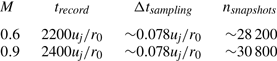
  $r=r_0$. The recording times, the sampling time and the number of snapshots captured are reported in table 2. They allow us to compute spectra up to ${St}=12.8$. The Fourier coefficients of the first five azimuthal modes $n_\theta =0\unicode{x2013}4$ (where $n_\theta$ is the azimuthal wavenumber) of the flow variables have been stored at a sampling Strouhal number $12.8$. Time spectra have been calculated using the Welch's method (Welch Reference Welch1967) considering segments of durations $40r_0 /u_j$ for ${M}=0.6$, and $75 r_0 / u_j$ for ${M}=0.9$, with $50\,\%$ overlap using a Hamming window. Frequency–axial wavenumber spectra have been obtained by computing spatial Fourier transforms of the time spectra in the axial direction between the nozzle-exit plane and the plate, using a Tukey (or tapered cosine) window and zero padding. The acoustic fields of the jets are obtained directly from the LES.
Table 2. Recording parameters: Mach number  ${M}=u_j/c_0$, recording time $t_{record}$, sampling time $\Delta t_{sampling}$, and number of snapshots captured $n_{snapshots}$.
3. Results for Mach number  $0.9$
$0.9$

3.1. Nozzle-exit conditions
The nozzle-exit profiles of the mean axial velocity and of the root mean square (r.m.s.) axial velocity fluctuations are plotted for the three jets at  ${M}=0.9$ in figure 1. In all cases, the mean velocity profiles are similar to those imposed at the effective pipe inlet at $z=-2r_0$. The r.m.s. profiles exhibit two local maximum values: one on the jet axis, and another near the pipe walls. The second one can be attributed to velocity fluctuations in the boundary layers. To determine the origin of the first one, GJW eigenfunctions predicted for the axisymmetric mode using a vortex-sheet model and normalized by the r.m.s. values at $r=0$ are plotted. More precisely, they correspond to those obtained for the duct-like GJW with zero group velocity for the first radial mode $n_r=1$ (Tam & Hu Reference Tam and Hu1989; Bogey Reference Bogey2021). Between $r=0$ and $r = r_0 - \delta _{BL}$, the r.m.s. velocity profiles are very similar to the GJW eigenfunctions, indicating that the fluctuations outside the boundary layers are due to GJWs. On the jet axis, the r.m.s. values are equal to $1.8\,\%$ of the jet velocity for M09BL05, $4.4\,\%$ for M09BL10, and $10\,\%$ for M09BL20. Near the pipe walls, they are equal to $1\,\%$, $4\,\%$ and $8\,\%$, respectively. Therefore, for the present jets, high-amplitude GJWs propagate upstream and excite the boundary layers, leading to disturbed exit conditions.

Figure 1. Nozzle-exit profiles of (a) mean axial velocity and (b) r.m.s. axial velocity fluctuations for M09BL05 (red), M09BL10 (blue) and M09BL20 (green); the dashed lines indicate normalized eigenfunctions of the duct-like GJW with zero group velocity (Tam & Hu Reference Tam and Hu1989; Bogey Reference Bogey2021) for  $n_\theta =0$ and $n_r=1$.
To characterize the nature of the high fluctuations levels near the pipe walls, the power spectral densities (PSD) of the radial velocity fluctuations computed at  $r=0.98r_0$ are represented as functions of the Strouhal number in figure 2. The contributions of the first two azimuthal modes to these spectra are also shown. High-amplitude peaks are observed at the same Strouhal numbers in the three cases, for the axisymmetric and the first helical modes. The peak frequencies and modal nature agree with those of the aeroacoustic resonant modes of the jets, which will be described in § 3.3 and § 3.4. Therefore, the nozzle-exit conditions of the jets differ significantly from those of initially fully laminar jets and even from those of unforced, initially disturbed jets whose nozzle-exit boundary-layer turbulence is dominated by high-order azimuthal modes ( ${n_\theta \gtrsim 10}$) (Bogey, Marsden & Bailly Reference Bogey, Marsden and Bailly2011b; Bogey & Sabatini Reference Bogey and Sabatini2019). On the contrary, they correspond to those of jets with boundary layer strongly forced at specific frequencies.

Figure 2. PSD of radial velocity fluctuations at  $z=0$ and $r=0.98 r_0$ for (a) M09BL05, (b) M09BL10 and (c) M09BL20 for the full spectra (black), $n_\theta = 0$ (red) and $n_\theta = 1$ (blue).
3.2. Flow field properties
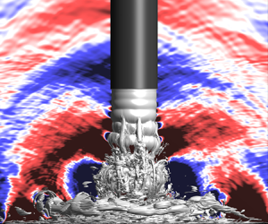
Snapshots of vorticity magnitude and pressure fluctuations are presented for the three jets in figure 3. In the vorticity fields, due to the laminar nozzle-exit conditions, shear-layer rolling-ups and vortex pairings are observed in all cases. For a thicker boundary layer, they occur later, leading to the generation of three-dimensional fine-scale turbulence farther downstream. In particular, for M09BL20 in figure 3(c), the mixing layers still contain large-scale axisymmetric vortical structures very near the plate.

Figure 3. Snapshots in the  $(z,r)$ plane of vorticity magnitude and pressure fluctuations for (a) M09BL05, (b) M09BL10 and (c) M09BL20. The colour scales range from $0.1 u_j / r_0$ to $10 u_j / r_0$ for vorticity, from black to white, and between ${\pm }0.015 p_0$ for pressure, from blue to red. The nozzle lips and the non-computed region in the pipe for $z<2r_0$ are in black.
In the pressure fields, the levels increase significantly for a thicker boundary layer. For M09BL05 in figure 3(a), no clear organization appears, and both low- and high-frequency waves are seen. By contrast, for M09BL10 and M09BL20 in figures 3(b) and 3(c), high-amplitude low-frequency spherical waves originating from the jet impingement region on the plate predominate. They are characterized by regularly-spaced wavefronts symmetrical with respect to the jet axis, indicating that the jets produce a tonal axisymmetric noise.
The shear-layer momentum thicknesses determined for the three impinging jets and for the corresponding free jets (Bogey Reference Bogey2022a) are plotted in figure 4(a). In both cases, in the near-nozzle region between  $z=0$ and $z\simeq 1.5r_0$, the shear layers spread more rapidly for a thinner exit boundary layer. Farther downstream, between $z=1.5r_0$ and $z=3r_0$, they develop at comparable rates, which results in similar shear-layer momentum thicknesses for the impinging jets, whereas thinner mixing layers are obtained for a thicker boundary layer for the free jets. Therefore, the development of the impinging jets is influenced significantly by the flat plate and by the high-amplitude upstream-propagating waves. Finally, between $z=3r_0$ and $z=6r_0$, for all jets, the mixing layers spread most slowly for the smallest boundary layer thickness, and at similar rates for the other two thicknesses.

Figure 4. Variations of (a) shear-layer momentum thickness for the impinging jets (solid lines) and free jets (dashed lines) at  ${M=0.9}$, with $\delta _{BL}=0.05r_0$ (red), $\delta _{BL}=0.1r_0$ (blue) and $\delta _{BL}=0.2r_0$ (green), and (b) r.m.s. axial velocity fluctuations at $r=r_0$ for M09BL05 (red), M09BL10 (blue) and M09BL20 (green).
The variations of the r.m.s. axial velocity fluctuations at  $r=r_0$ for the impinging jets are represented in figure 4(b). In all cases, the r.m.s. velocity fluctuations first increase strongly due to the amplification of the shear-layer instability waves, reach maximum values between $22\,\%$ and $26\,\%$ of the jet velocity, and then decrease down to the plate. For M09BL10 and M09BL20, oscillations are observed between $z=3r_0$ and $z=6r_0$. As will be shown in § 3.4, they are due to constructive and destructive interferences between upstream- and downstream-propagating waves (Panda Reference Panda1999; Gojon et al. Reference Gojon, Bogey and Marsden2016).
3.3. Near-nozzle pressure spectra
The pressure spectra computed at  $z=0$ and $r=1.5 r_0$ are plotted as functions of the Strouhal number in figure 5. For comparison, spectra obtained for the corresponding free jets (Bogey Reference Bogey2022a) are also represented. For the impinging jets, the broadband noise levels are higher for a thicker boundary layer, increasing approximately by $10\ \mathrm {dB}$ between M09BL05 and M09BL20. As expected, tones emerge, at frequencies that are very similar for the three boundary-layer thicknesses. The strongest ones appear at Strouhal numbers ${St}\simeq 0.32$, $0.41$, $0.68$ and $0.82$. In all cases, the dominant tone is found at ${St}\simeq 0.41$, as in the numerical study by Varé & Bogey (Reference Varé and Bogey2022) and the experiments by Panickar & Raman (Reference Panickar and Raman2007) for jets at ${M}=0.9$ impinging on a plate located at the same nozzle-to-plate distance as the present jets.

Figure 5. Sound pressure levels (SPL) at  $z=0$ and $r=1.5r_0$ for the impinging jets (solid lines) and free jets (dashed lines) at ${M}=0.9$, with $\delta _{BL}=0.05r_0$ (red), $\delta _{BL}=0.1r_0$ (blue) and $\delta _{BL}=0.2r_0$ (green).
The Strouhal numbers  ${St}\simeq 0.41$ and $0.68$ are close to those of the peaks in the free jet spectra. Those peaks were attributed to resonant GJWs propagating with opposite group velocities (Schmidt et al. Reference Schmidt, Towne, Colonius, Cavalieri, Jordan and Brès2017; Towne et al. Reference Towne, Cavalieri, Jordan, Colonius, Schmidt, Jaunet and Brès2017). At the peak frequencies, the levels are much stronger for the impinging jets than for the free jets, especially in the case of the thicker boundary layer. Thus at the Strouhal number ${St}\simeq 0.41$ of the dominant tone, the difference in peak level is $20 \ \mathrm {dB}$ for $\delta _{BL}=0.05r_0$, $33 \ \mathrm {dB}$ for $\delta _{BL}=0.1r_0$, and $38 \ \mathrm {dB}$ for $\delta _{BL}=0.2r_0$.
For the impinging jets, the tone amplitudes are higher for a thicker boundary layer. In particular, the amplitude of the dominant tone increases by  $19\ \mathrm {dB}$ between M09BL05 and M09BL10, and by $7\ \mathrm {dB}$ between M09BL10 and M09BL20. The dominant tone thus emerges by more than $20\ \mathrm {dB}$ with respect to the broadband noise levels in the two latter cases, indicating that the jets are highly resonant. The amplitude of the tone at ${St}\simeq 0.32$ increases by $4\ \mathrm {dB}$ between M09BL05 and M09BL10, and by $13\ \mathrm {dB}$ between M09BL10 and M09BL20. Therefore, this tone emerges strongly for the jet with M09BL20, but more weakly for the two other ones. Finally, the tone at ${St}\simeq 0.68$ is the second strongest one for the jet with the thinnest boundary layers, but not for the two others.
The Strouhal numbers of the two dominant tones, i.e.  ${St}\simeq 0.32$ and $0.41$, are consistent with the Strouhal numbers
 \begin{equation} {St} = N\,\dfrac{D/L}{u_j / u_c + u_j/ c_0} , \end{equation}
determined using an aeroacoustic feedback model (Ho & Nosseir Reference Ho and Nosseir1981; Powell Reference Powell1988). The latter are equal to  ${St}\simeq 0.35$ and $0.46$ for feedback loops of orders $N=3$ and $4$, considering that the vortical structures are convected at velocity $u_c=0.5u_j$. Thus the two strongest tones appear to result from two different feedback loops establishing between the nozzle and the plate. It can be noted that the convection speed $u_c=0.5u_j$ was obtained directly from the frequency–axial wavenumber spectra shown later, in § 3.4. It corresponds to the phase velocity of the flow fluctuations propagating downstream at the tone frequencies. It is close to the average convection speeds computed in the mixing layers between the nozzle and the plate using velocity cross-correlations, which range between $0.47u_j$ and $0.61u_j$ depending on the nozzle-exit boundary layer.
The contributions of the first four azimuthal modes  $n_\theta =0\unicode{x2013}3$ to the near-nozzle pressure spectra for the three impinging jets are represented in figures 6(a)–6(c). In all cases, these azimuthal modes contribute significantly to the full spectra. The dominant modes are the mode $n_\theta =0$ for ${St}\leq 0.41$, and the mode $n_\theta =1$ for $0.41<{St}\leq 0.7$. Thus the two strong tones at ${St}\simeq 0.32$ and $0.41$, referred to as $N_3$ and $N_4$ tones in the following, are associated with the mode $n_\theta =0$, and the tone at ${St}\simeq 0.68$ is linked to the mode $n_\theta =1$. The first two harmonics $2N_4$ and $3N_4$ of the strongest tone are also observed for M09BL10 and M09BL20 in figures 6(b,c) for $n_\theta =0$.

Figure 6. Sound pressure levels at  $z=0$ and $r=1.5r_0$ for (a) M09BL05, (b) M09BL10 and (c) M09BL20, for the full spectra (black), $n_\theta = 0$ (red), $n_\theta = 1$ (blue), $n_\theta = 2$ (green) and $n_\theta = 3$ (yellow).
The sound pressure levels of the tones  $N_4$ and $N_3$ are represented as functions of the boundary-layer thickness in figure 7. For the strongest tone, $N_4$, the level is $26\ \mathrm {dB}$ higher for M09BL20 than for M09BL05, while for the tone $N_3$, it increases by $17\ \mathrm {dB}$ between M09BL05 and M09BL20.

Figure 7. Sound pressure levels at  $z=0$ and $r=1.5r_0$ of the tones $N_3$ and $N_4$ as functions of the boundary-layer thickness for the impinging jets at ${M}=0.9$.
3.4. Feedback loop properties
At the frequencies of the two dominant tones  $N_4$ and $N_3$, the upstream- and downstream-propagating waves involved in the feedback loops are expected to lead to constructive and destructive interferences at specific locations in the flow. To visualize such interferences, the pressure levels obtained at the two tone frequencies for the axisymmetric mode for the three jets are shown in figure 8. In all cases, high-energy spots regularly spaced in the axial direction are observed between the nozzle and the plate. They form standing wave patterns similar to those found previously in screeching jets (Panda Reference Panda1999; Gojon & Bogey Reference Gojon and Bogey2017b) and in resonant impinging jets (Gojon et al. Reference Gojon, Bogey and Marsden2016; Bogey & Gojon Reference Bogey and Gojon2017; Varé & Bogey Reference Varé and Bogey2022). For all boundary-layer thicknesses, four and three spots are found between the nozzle and the plate for the tones $N_4$ and $N_3$, respectively. The number of spots agrees with the resonance mode order obtained previously using the aeroacoustic feedback model (3.1), as was the case in the study by Gojon et al. (Reference Gojon, Bogey and Marsden2016). For the strongest tone, $N_4$, it also matches the number of oscillations in the r.m.s. velocity profiles at $r=r_0$ for M09BL10 and M09BL20 in figure 4(b).

Figure 8. Sound pressure levels at the frequencies of the tones (a–c)  $N_4$ and (d–f) $N_3$ for (a,d) M09BL05, (b,e) M09BL10 and (c,f) M09BL20, for $n_\theta =0$. The colour scale ranges over $20 \ \mathrm {dB}$ from blue to yellow, with maximum values in yellow.
To further characterize the resonances and the different waves propagating at the tone frequencies, the frequency–wavenumber spectra of the pressure fluctuations computed between the nozzle and the plate for the axisymmetric mode on the jet axis and in the shear layers are represented in figures 9(a)–9(f) as functions of the axial wavenumber  $k_z$ and the Strouhal number. The line $\omega /k_z = 0.5 u_j$ and the sonic line $\omega /k_z = -c_0$, where $\omega = 2 {\rm \pi}f$ is the angular frequency, the dispersion curve of the first radial mode of the GJW for a vortex-sheet model for $n_\theta =0$ (Tam & Hu Reference Tam and Hu1989; Towne et al. Reference Towne, Cavalieri, Jordan, Colonius, Schmidt, Jaunet and Brès2017; Bogey Reference Bogey2021), and the Strouhal numbers of the tones $N_4$ and $N_3$, are also depicted. In the mixing layers, in figures 9(d)–9(f), in all cases, high levels are observed for positive wavenumbers near the line $\omega /k_z = 0.5 u_j$. They can be associated with the turbulent structures convected in the downstream direction at a velocity close to half of the jet velocity. At the tone Strouhal numbers, the strongest levels appear near the line $\omega /k_z = 0.5 u_j$ mentioned above, but also close to the dispersion curve of the GJWs near the sonic line for negative wavenumbers. Therefore, the two dominant tones are generated by feedback loops closed by upstream-propagating free-stream GJWs (Towne et al. Reference Towne, Cavalieri, Jordan, Colonius, Schmidt, Jaunet and Brès2017; Bogey Reference Bogey2021). On the jet axis, in figures 9(a)–9(c), the frequency–wavenumber spectra differ slightly from those in the mixing layers. In particular, the contributions of the structures convected in the jet shear layers are weaker, whereas those of the GJWs are stronger. This is consistent with the eigenfunctions of the Kelvin–Helmholtz instability waves and of the GJWs (Tam & Hu Reference Tam and Hu1989).

Figure 9. Frequency–wavenumber spectra of the pressure fluctuations computed at (a–c)  $r=0$ and (d–f) $r=r_0$ for (a,d) M09BL05, (b,e) M09BL10 and (c,f) M09BL20, for $n_\theta =0$. The red long-dashed line indicates the dispersion curve of the first radial mode of the GJW for a vortex-sheet model. The red solid line indicates $\omega / k_z = 0.5u_j$, and the red dotted line indicates $\omega / k_z = - c_0$. The red dashed horizontal lines indicate the Strouhal numbers of the tones $N_3$ and $N_4$. The colour scale ranges logarithmically from the minimal to the maximal values, from blue to yellow.
The stronger tone amplitudes for a thicker boundary layer are most probably related to a change in the gain parameters of the feedback loops. These parameters, introduced by Powell (Reference Powell1961) and described by Edgington-Mitchell (Reference Edgington-Mitchell2019), are the gain in amplitude of the instability waves between the nozzle and the plate, the efficiency of the noise generation mechanisms near the plate, the efficiency of the transmission of the upstream-travelling waves from the plate to the nozzle, and the efficiency of the receptivity process (Barone & Lele Reference Barone and Lele2005; Karami et al. Reference Karami, Stegeman, Ooi, Theofilis and Soria2020) at the nozzle lip. Assuming that the receptivity process depends only on the nozzle geometry and that the upstream-travelling waves are GJWs propagating without significant amplitude variations (Tam & Hu Reference Tam and Hu1989; Bogey Reference Bogey2021), the increase of the tone amplitudes for  $n_\theta =0$ as the jet boundary layer is thicker can be attributed to differences in the noise generation mechanisms near the plate and in the instability wave amplification processes. This is discussed in what follows by examining the predominance of the axisymmetric flow fluctuations in the mixing layers and their nozzle-to-plate gains in amplitude.
3.5. Predominance of the axisymmetric flow fluctuations in the mixing layers
The strength and persistence of axisymmetric flow fluctuations in the jet mixing layers from the nozzle down to the plate are investigated. For that, the r.m.s. values of the radial velocity fluctuations obtained at  $r=r_0$ for the full signals, for $n_\theta =0$, and for the axisymmetric velocity fluctuations of aerodynamic nature only are plotted for the three jets in figures 10(a)–10(c). The fluctuations of aerodynamic nature are obtained by filtering out the upstream-propagating fluctuations and the downstream-propagating acoustic waves in the radial velocity signals using a frequency–wavenumber filtering procedure described in Appendix B. In all cases, in figure 10(a), the full velocity fluctuations increase rapidly, reach peak values approximately equal to $20\,\%$ of the jet velocity at $z\simeq 1.5r_0$ for M09BL05, at $z\simeq 2r_0$ for M09BL10, and near the plate for M09BL20, and then decrease down to the plate. Compared with the levels obtained from the full signals, those for the mode $n_\theta =0$ in figure 10(b) are very similar for M09BL20 but are lower for thinner boundary layers. This is notably true near the plate at $z=5r_0$, where the levels are equal to $20\,\%$ of the jet velocity for M09BL20, $9\,\%$ for M09BL10, and only $2\,\%$ for M09BL05. Therefore, for M09BL20, axisymmetric structures dominate strongly in the mixing layers down to the flat plate. They still contain a significant amount of energy for M09BL10, but are weak for M09BL05. These results are consistent with the variations of the amplitudes of the tones for $n_\theta =0$ in figure 7. Moreover, oscillations are observed for M09BL10 and M09BL20 in the r.m.s. profiles. They can be attributed to the interferences between upstream- and downstream-propagating waves. Finally, the r.m.s. profiles of the aerodynamic velocity fluctuations for $n_\theta = 0$ in figure 10(c) are similar to those obtained without filtering in figure 10(b). Nevertheless, they do not contain oscillations since the upstream-propagating fluctuations have been filtered out. After the initial increase near the nozzle exit, the profiles exhibit a peak and then decrease. For a thicker boundary layer, the peak value is reached farther downstream and is higher, due to the slower shear-layer laminar–turbulent transition. Consequently, near the plate, the axisymmetric turbulent structures contain more energy, which most likely contributes to increase the amplitudes of the tones for $n_\theta =0$.

Figure 10. Variations of r.m.s. radial velocity fluctuations obtained for (a) the full signals, (b)  $n_\theta =0$, and (c) the fluctuations of aerodynamic nature for $n_\theta =0$, at $r=r_0$ for M09BL05 (red), M09BL10 (blue) and M09BL20 (green).
3.6. Amplification and gain in amplitude of the axisymmetric aerodynamic velocity fluctuations at the tone frequencies
As was done by Varé & Bogey (Reference Varé and Bogey2023) for impinging jets at different Mach numbers, the gain in amplitude of the axisymmetric shear-layer instability waves between the nozzle and the plate was first estimated using inviscid spatial LSA from the LES mean flow fields, as reported in Appendix A. At the tone frequencies, the gains obtained in this way are very similar for the three boundary-layer thicknesses. Given the limitations of LSA due to the inviscid and linear assumptions, the gain in amplitude of the instability waves was then calculated directly from the velocity fluctuations of aerodynamic nature obtained at  $r=r_0$.
The PSD computed from these fluctuations for  $n_\theta =0$ are represented in the $(z,{St})$ plane in figure 11. For comparison, the spectra estimated for the corresponding free jets Bogey (Reference Bogey2021) are also shown. The Strouhal numbers of the most amplified instability waves evaluated using LSA and of the dominant tones $N_4$ and $N_3$ are depicted for the impinging jets. For the free jets, in figures 11(d)–11(f), several high-energy spots are found around specific frequencies. They result from the coupling between the free-stream upstream-propagating GJWs and the shear-layer instability waves near the nozzle, as shown by Bogey (Reference Bogey2022a) for free jets with fully laminar exit boundary layers. For a thicker boundary layer, they are located farther downstream, due to the reduction of the peak instability growth rate. For the impinging jet with $\delta _{BL}=0.05r_0$, in addition to the spots, stripes extending from the nozzle down to the plate are seen at the tone Strouhal numbers in figure 11(a). Their levels increase with the axial distance and are maximum near the plate. Similar results are obtained for M09BL10 and M09BL20 in figures 11(b) and 11(c). In these cases, however, the stripes at the tone Strouhal numbers emerge more strongly, and additional ones appear at the harmonics of the tone frequencies. Therefore, for all impinging jets, axisymmetric aerodynamic fluctuations develop in the shear layers from the nozzle to the plate at the tone frequencies. Nevertheless, as previously pointed out, they contain much more energy as the nozzle-exit boundary layer is thicker.

Figure 11. PSD of radial velocity fluctuations of aerodynamic nature normalized by  $u_j$ for $n_\theta =0$, at $r=r_0$, for (a–c) impinging jets and (d–f) free jets at ${M}=0.9$, with (a,d) $\delta _{BL}=0.05r_0$, (b,e) $\delta _{BL}=0.1r_0$ and (c,f) $\delta _{BL}=0.2r_0$. The red dashed lines indicate the Strouhal numbers of the tones $N_4$ and $N_3$. The red solid lines indicate the most unstable Strouhal numbers for $n_\theta =0$ according to LSA. The colour scales range logarithmically from $(5D/u_j)\times 10^{-5}$ to $(D/u_j) \times 10^{-1}$, from blue to yellow.
Focusing on the amplification of the flow fluctuations at the tone frequencies, the PSD of the aerodynamic fluctuations obtained at  $r=r_0$ for $n_\theta =0$ at the frequencies of the tones $N_4$ and $N_3$ for the three impinging jets are plotted in figure 12 using a logarithmic scale. They are normalized by their values at $z=0.5r_0$. In all cases, overall, the levels increase with the axial distance, except very near the plate. Between $z=3r_0$ and $z=5r_0$, they are significantly higher for a thicker boundary layer.

Figure 12. PSD of the axisymmetric velocity fluctuations of aerodynamic nature at  $r=r_0$ normalized by the values of the PSD at $z=0.5r_0$ at the frequencies of the tones (a) $N_4$ and (b) $N_3$ for M09BL05 (red), M09BL10 (blue) and M09BL20 (green).
Finally, the nozzle-to-plate gains in amplitude of the flow fluctuations at  $r=r_0$ for $n_\theta = 0$ are estimated by computing the square root of the ratio between the PSD of the aerodynamic velocity fluctuations at $z=4.5 r_0$ and at $z=0.5 r_0$. The bounds are chosen arbitrarily, but similar results are obtained for other ones. The nozzle-to-plate gains thus calculated at the Strouhal numbers of the tones $N_4$ and $N_3$ are plotted as functions of the boundary-layer thickness in figure 13. For completeness, the gains obtained for Strouhal numbers between $0.1$ and $1.6$ are provided and compared with those predicted using LSA in Appendix B. For both tone frequencies, in figure 13, the gain is stronger for a thicker boundary layer. For the dominant tone $N_4$, the gains for M09BL10 and M09BL20 are approximately two and three times greater than that for M09BL05. For the tone $N_3$, the gains for M09BL10 and M09BL20 are $1.5$ and $1.8$ times higher than that for M09BL05. Thus the aerodynamic fluctuations developing at the tone frequencies in the jet shear layers are more amplified between the nozzle and the plate for a thicker boundary layer. This most likely promotes the emergence of stronger tones.

Figure 13. Gains in amplitude of the axisymmetric flow velocity fluctuations at  $r=r_0$ between $z=0.5r_0$ and $z=4.5r_0$ at the frequencies of the tones $N_4$ and $N_3$ as functions of the boundary-layer thickness for the jets at ${M}=0.9$.
4. Results for Mach number $0.6$

4.1. Nozzle-exit conditions
The nozzle-exit profiles of the mean axial velocity and of the r.m.s. values of the axial velocity fluctuations obtained for the three jets at  ${M}=0.6$ are plotted in figure 14. In all cases, the mean velocity profile is similar to the Blasius laminar boundary-layer profile imposed at the effective pipe inlet at $z=-2r_0$. The r.m.s. velocity values between the jet axis and the pipe walls are low, ranging between only $0.2\,\%$ and $0.7\,\%$ of the jet velocity for the three boundary-layer thicknesses. This indicates that the nozzle-exit boundary layers are fully laminar (Zaman Reference Zaman1985a,Reference Zamanb; Bogey & Bailly Reference Bogey and Bailly2010). This result is different from that for the jets at ${M}=0.9$, shown to be significantly excited by GJWs in § 3.1.

Figure 14. Nozzle-exit profiles of (a) mean and (b) r.m.s. axial velocity for M06BL05 (red), M06BL10 (blue) and M06BL20 (green).
4.2. Flow field properties
Snapshots of vorticity magnitude and pressure fluctuations obtained for the three jets are displayed in figure 15. In the vorticity fields, vortices appear in the jet shear layers, close to the nozzle, at  $z\simeq 0.5 r_0$ for M06BL05, at $z\simeq r_0$ for M06BL10, and at $z\simeq 2 r_0$ for M06BL20. Farther downstream, vortex pairings occur. For M06BL05 and M06BL10, they lead to the generation of fine-scale turbulent structures in the mixing layers. By contrast, for M06BL20, the pairings happen very near the plate, resulting in the impingement of only large-scale coherent structures. Regarding the pressure fields, they do not show a clear organization, and exhibit acoustic waves of similar amplitude for the three jets.

Figure 15. Snapshots in the  $(z,r)$ plane of vorticity magnitude and pressure fluctuations for (a) M06BL05, (b) M06BL10 and (c) M06BL20. The colour scales range from $0.1 u_j / r_0$ to $10 u_j / r_0$ for vorticity, from black to white, and between ${\pm }0.005 p_0$ for pressure, from blue to red. The nozzle lips and the non-computed region in the pipe for $z<2r_0$ are in black.
The shear-layer momentum thicknesses obtained for the impinging jets and the corresponding free jets (Bogey Reference Bogey2022a) are plotted in figure 16(a). In both cases, the mixing layers develop more rapidly for a thinner boundary layer, leading to thicker shear layers between  $z=r_0$ and $z=4r_0$. For all boundary-layer thicknesses, the variations determined for the impinging jets are very similar to those for the free jets. This was not the case for the impinging jets at ${M}=0.9$, appearing to be significantly influenced by the plate and by the high-amplitude acoustic waves. The variations of the r.m.s. axial velocity fluctuations at $r=r_0$ obtained for the full signals and for the axisymmetric fluctuations of aerodynamic nature are plotted in figures 16(b,c). As for the jets at ${M}=0.9$, the aerodynamic fluctuations are estimated by filtering out the upstream-propagating disturbances and the downstream-propagating acoustic waves using the frequency–wavenumber filtering described in Appendix B. In all cases, in figure 16(b), the r.m.s. velocity values first increase sharply in the near-nozzle region, reach peak values equal to approximately $22\,\%$ of the jet velocity, and then decrease down to the plate. The peak values are obtained farther downstream for a thicker boundary layer, yielding higher levels near the plate. In figure 16(c), the variations of the levels of the axisymmetric aerodynamic fluctuations are similar to those of the full signals. However, the levels are lower. Near the plate at $z=5r_0$, in particular, they are equal to $12\,\%$ of the jet velocity for M06BL20, $4\,\%$ for M06BL10, and $2\,\%$ for M06BL05. Therefore, much more energy is contained in the axisymmetric structures impinging on the plate for a thicker boundary layer.

Figure 16. Variations of (a) shear-layer momentum thickness for the impinging jets (solid lines) and free jets (dashed lines), and r.m.s. radial velocity fluctuations at  $r=r_0$ obtained for (b) the full signals and (c) the fluctuations of aerodynamic nature for $n_\theta =0$ for M06BL05 (red), M06BL10 (blue) and M06BL20 (green).
4.3. Near-nozzle pressure spectra
The pressure spectra obtained at  $z=0$ and $r=1.5 r_0$ for the impinging jets and the corresponding free jets (Bogey Reference Bogey2022a) are plotted as functions of the Strouhal number in figure 17. For all impinging jets, a low-frequency broadband hump centred around ${St}\simeq 0.4$ is found. Its amplitude is higher for a thicker boundary layer, and increases by approximately $2\ \mathrm {dB}$ between M06BL05 and M06BL10, and by $12\ \mathrm {dB}$ between M06BL10 and M06BL20. The noise levels are stronger for the impinging jets than for the free ones. For $0.2\lesssim {St} \lesssim 0.8$, in particular, the increase is about $10 \ \mathrm {dB}$ for $\delta _{BL}=0.05r_0$ and $\delta _{BL}=0.1r_0$, and $15 \ \mathrm {dB}$ for $\delta _{BL}=0.2r_0$. For M06BL20, small narrow peaks are visible at Strouhal numbers ${St}\simeq 0.66$, $0.77$ and $0.89$. As will be shown in § 4.5, they are linked to aeroacoustic feedback loops establishing between the nozzle and the plate. However, the strongest one at ${St}\simeq 0.77$ emerges only by $3\ \mathrm {dB}$ from the broadband hump levels. The frequencies of the three peaks are consistent with the Strouhal numbers ${St}\simeq 0.64$, $0.77$ and $0.9$ predicted by the aeroacoustic feedback model (3.1) for $N=6$, $7$ and $8$, assuming a convection velocity $u_c=0.5u_j$. This suggests that the peaks are due to feedback loops of three different orders establishing between the nozzle and the plate.

Figure 17. Sound pressure levels at  $z=0$ and $r=1.5r_0$ for the impinging jets (solid lines) and free jets (dashed lines) at ${M}=0.6$, with $\delta _{BL}=0.05r_0$ (red), $\delta _{BL}=0.1r_0$ (blue) and $\delta _{BL}=0.2r_0$ (green). The grey dashed lines indicate the Strouhal numbers of the narrow peaks for M06BL20.
The contributions of the first five azimuthal modes to the near-nozzle pressure spectra are represented in figures 18(a)–18(c). For the three jets, the low-frequency hump in the spectra is associated with the axisymmetric mode. For M06BL05 in figure 18(a), the spectra exhibit small peaks for the modes  $n_\theta =1$, $2$,
$2$,  $3$ and $4$ at ${St}\simeq 1.4$, $2$,
$2$,  $2.4$ and $2.8$, respectively. Their frequencies correspond to those of the acoustic peaks found near the nozzle of a free jet at ${M}=0.6$ (Bogey Reference Bogey2021), which have been associated with the first least-dispersed GJWs for $n_\theta =1$, $2$,
$2$,  $3$ and $4$. For M06BL10 in figure 18(b), two narrow peaks can also be seen at ${St}\simeq 1$ and ${St}\simeq 1.2$ for $n_\theta =0$. Their amplitudes are relatively low, but they will be associated with feedback phenomena in what follows. For M06BL20 in figure 18(c), the small peaks at ${St}\simeq 0.66$, $0.77$ and $0.89$ are associated with the axisymmetric mode.

Figure 18. Sound pressure levels at  $z=0$ and $r=1.5r_0$ for (a) M06BL05, (b) M06BL10 and (c) M06BL20, for the full spectra (black), $n_\theta = 0$ (red), $n_\theta = 1$ (blue), $n_\theta = 2$ (green), $n_\theta = 3$ (yellow) and $n_\theta = 4$ (cyan). The grey dashed lines indicate the Strouhal numbers of the small peaks for M06BL10 and M06BL20.
The small peaks for M06BL10 and M06BL20 hardly emerge from the broadband components in the spectra. Therefore, to extract and make these peaks more visible, a spectral proper orthogonal decomposition (SPOD) (Towne et al. Reference Towne, Schmidt and Colonius2018; Schmidt & Colonius Reference Schmidt and Colonius2020) has been applied to the axisymmetric pressure fluctuations of the impinging jets M06BL10 and M06BL20, as described in Appendix C. The pressure fields associated with the first SPOD mode, i.e. the mode with the highest energy content, have been reconstructed in the frequency domain (Nekkanti & Schmidt Reference Nekkanti and Schmidt2021). The spectra computed at  $z=0$ and $r=1.5r_0$ are plotted with the full sound spectra for $n_\theta =0$ in figures 19(a) and 19(b). In both cases, the levels for the first SPOD mode are lower than those for the full spectra. The small peaks previously mentioned, indicated by dashed lines, are visible in both spectra. However, they emerge more significantly from the broadband levels in the spectra associated with the first SPOD mode. In particular, the strongest peak for M06BL20 at ${St}\simeq 0.77$ emerges by about $6\ \mathrm {dB}$ for the total spectrum, and $12\ \mathrm {dB}$ for the spectrum determined from the SPOD. This provides further evidence that the jets M06BL10 and M06BL20 are weakly resonant.

Figure 19. Sound pressure levels at  $z=0$ and $r=1.5r_0$ for $n_\theta =0$ for (a) M06BL10 and (b) M06BL20 for the full spectra (black) and the first SPOD mode (red). The grey dashed lines indicate the Strouhal numbers of the peaks in the near-nozzle spectra.
4.4. Velocity spectra
The spectra of the radial velocity fluctuations of aerodynamic nature obtained for the three impinging jets and the corresponding free jets (Bogey Reference Bogey2022a) for  $n_\theta =0$ at $r=r_0$ are represented as functions of the axial position and Strouhal number in figures 20(a)–20(f). For the impinging jets, the frequencies of the jet initial most-amplified instability waves obtained at $z=0.1 r_0$ for $n_\theta = 0$ using LSA, half of these frequencies, and the frequencies of the small peaks found in the near-nozzle spectra for M06BL10 and M06BL20, are also depicted. For the free jets, in figures 20(d)–20(f), the highest levels are found in two spots centred, e.g. for $\delta _{BL} = 0.1 r_0$, around $z\simeq 1.5r_0$ and ${St}\simeq 2.5$, and around $z\simeq 2.5 r_0$ and ${St}\simeq 1.3$. They are associated with the shear-layer roll-ups and vortex pairings. For a thicker boundary layer, due to the reduction of instability growth rates, the spots are located farther downstream. In particular, the second spot is observed at $z\simeq 1.5r_0$ for $\delta _{BL}=0.05r_0$, at $z\simeq 2.5r_0$ for $\delta _{BL}=0.1r_0$, and at $z\simeq 4r_0$ for $\delta _{BL}=0.2r_0$. For $\delta _{BL}=0.05 r_0$ and $\delta _{BL} = 0.1 r_0$, farther downstream, the spectra become broadband, which indicates that the axisymmetric vortices initially formed in the mixing layers break up, generating small-scale turbulence. For the impinging jets, in figures 20(a)–20(c), spots very similar to those observed for the free jets are seen in the spectra. Moreover, for M06BL10 and M06BL20, the second spots contain stripes of significant amplitude between $z\simeq 1.5r_0$ and $z=5.5r_0$. Their Strouhal numbers correspond to those of the small peaks emerging in the near-nozzle spectra. Consequently, these results indicate that axisymmetric structures persist over large distances at the peak frequencies, and therefore that resonant phenomena occur for M06BL10 and M06BL20.

Figure 20. PSD of radial velocity fluctuations of aerodynamic nature normalized by  $u_j$ for $n_\theta =0$, at $r=r_0$, for (a–c) impinging jets and (d–f) free jets at ${M}=0.6$, with (a,d) $\delta _{BL}=0.05r_0$, (b,e) $\delta _{BL}=0.1r_0$ and (c,f) $\delta _{BL}=0.2r_0$. The red triangles indicate the most unstable Strouhal numbers at $z=0.1r_0$ predicted by LSA for $n_\theta =0$, and half of these Strouhal numbers. The red dashed lines indicate the Strouhal numbers of the peaks in the near-nozzle spectra for M06BL10 and M06BL20. The colour scales range logarithmically from $(5D/u_j)\times 10^{-5}$ to $(D/u_j) \times 10^{-1}$, from blue to yellow.
The spectra of the radial velocity fluctuations at  $z=3 r_0$ and $r=r_0$ for $n_\theta =0$ are plotted for all jets in figure 21. Overall, for all thicknesses, the spectra obtained for the impinging and free jets are very similar. They are mostly broadband, exhibiting large humps associated with shear-layer roll-ups and vortex pairings for M06BL10 and M06BL20. For the latter jets, tiny peaks are also visible at the Strouhal numbers of the peaks in the near-nozzle spectra. Those for M06BL20 emerge more clearly than those for M06BL10. This suggests that an increase in boundary-layer thickness promotes the establishment of the resonant loops.

Figure 21. PSD of aerodynamic radial velocity fluctuations at  $z=3 r_0$ and $r=r_0$ for $n_\theta=0$ for the jets at ${M}=0.6$ with (a) $\delta _{BL}=0.05r_0$, (b) $\delta _{BL}=0.1r_0$ and (c) $\delta _{BL}=0.2r_0$, for the impinging jets (red) and free jets (blue). The grey dashed lines indicate the Strouhal numbers of the small peaks in the near-nozzle spectra for M06BL10 and M06BL20.
4.5. Feedback loop properties
To provide further evidence that the jet M06BL20 is resonant, the sound pressure levels obtained for the three impinging jets for  $n_\theta =0$ at ${St}\simeq 0.77$, i.e. the Strouhal number of the strongest small peak in the near-nozzle spectrum for M06BL20, are shown in the $(z,r)$ plane in figure 22. In all cases, the highest levels are located in the mixing layers and in the wall jets. For M06BL05 and M06BL10, the pressure fields do not exhibit a specific organization. For M06BL20, on the contrary, spots of high energy regularly spaced in the axial direction can be seen between the nozzle and the plate on both sides of the shear layers. They are similar to those observed for the jets at ${M} = 0.9$ in figure 8. Thus for this jet, interactions between upstream- and downstream-propagating waves occur at the peak frequency, indicating that the peak results from a feedback loop establishing between the nozzle and the plate. Between $z=0.8r_0$ and $z=3.7r_0$, the number of spots is equal to $3$. Therefore, the wavelength of the standing wave formed by the spots is $\lambda _{sw}\simeq 0.97 r_0$. This value is consistent with the wavelength
 \begin{equation} \lambda_{sw}= \dfrac{D}{{St}\,(u_j/u_c + u_j/c_0)} = 0.9r_0 , \end{equation}
obtained for a standing wave with downstream and upstream components travelling at  $u_c=0.5u_j$ and $c_0$ (Panda Reference Panda1999).

Figure 22. Sound pressure levels at  ${St}\simeq 0.77$ for (a) M06BL05, (b) M06BL10 and (c) M06BL20, for $n_\theta =0$. The colour scale ranges from $110 \ \mathrm {dB}$ to $170 \ \mathrm {dB}$, from blue to yellow.
The frequency–wavenumber spectrum of the pressure fluctuations computed at  $r=r_0$ for the axisymmetric mode between $z=0$ and $z=6r_0$ for M06BL20 is represented in figure 23. The lines $\omega /k_z=0.5u_j$ and $\omega /k_z=-c_0$, the dispersion curve of the first radial mode of the GJWs for $n_{\theta}=0$, the first least-dispersed GJW, and the Strouhal numbers of the peaks in the near-nozzle spectrum for M06BL20, are also indicated. Strong levels are obtained near the line $\omega /k_z=0.5u_j$ and are due to the flow structures convected downstream. The highest levels are observed at the Strouhal numbers of first two near-nozzle peaks, ${St}=0.66$ and ${St}=0.77$. They extend over a broad range of wavenumbers. In particular, non-negligible levels are found for negative wavenumbers near the dispersion curve. This provides additional evidence that waves propagate downstream and upstream at specific frequencies in the mixing layers. The two Strouhal numbers are significantly lower than the Strouhal number of the first least-dispersed GJW, which is ${St}=1$. However, they lie in the range of the free-stream GJWs propagating at a velocity very close to the ambient speed of sound, suggesting that the feedback loops are closed by these waves.

Figure 23. Frequency–wavenumber spectrum of the pressure fluctuations computed for  $n_\theta =0$ at $r=r_0$ for M06BL20. The red solid line indicates $\omega / k_z = 0.5 u_j$, and the red dotted line indicates $\omega / k_z = - c_0$. The red long-dashed line indicates the dispersion curve of the GJWs for a vortex-sheet model. The red dot indicates the first least-dispersed GJW. The red horizontal dashed lines indicate the Strouhal numbers of the peaks for M06BL20. The colour scale ranges logarithmically from the minimal to the maximal values, from blue to yellow.
4.6. Gain in amplitude of the axisymmetric aerodynamic velocity fluctuations
The emergence of acoustic peaks for a thicker boundary layer may be due to a greater amplification of the axisymmetric instability waves between the nozzle and the plate. To discuss this, the nozzle-to-plate gain in amplitude of the axisymmetric radial velocity fluctuations of aerodynamic nature are estimated by computing the ratios between the PSD of the velocity fluctuations of aerodynamic nature at  $z = 0.5r_0$ and at $z = 4.5r_0$, as for the jets at ${M}=0.9$ in § 3.6. The gains obtained in this way for the three boundary-layer thicknesses for Strouhal numbers between $0.1$ and $1.6$ are reported in Appendix B in figure 28(a). They agree fairly well, in terms of levels and variations, with those estimated using LSA, provided in Appendix A in figure 26(a), despite the limitations of the LSA.
The gain obtained at the frequency of the strongest narrow small peak in the near-nozzle spectrum for M06BL20 is plotted as a function of the boundary-layer thickness in figure 24. For M06BL20, it is  $2$ times higher than that for M06BL10 and $3.3$ higher than that for M06BL05. Therefore, at the peak frequency, the flow fluctuations for $n_\theta =0$ are more amplified between the nozzle and the plate for a thicker boundary layer. This and the greater predominance of axisymmetric fluctuations near the plate for a thicker boundary layer in figure 16 most likely contribute to the establishment of feedback loops for M06BL20.

Figure 24. Gain in amplitude of the aerodynamic axisymmetric flow velocity fluctuations at  $r=r_0$ between $z=0.5r_0$ and $z=4.5r_0$ at ${St}=0.77$, i.e. the Strouhal number of the strongest small peak in the near-nozzle spectrum for M06BL20, as a function of the boundary-layer thickness for the jets at ${M}=0.6$.
5. Conclusions
In this paper, the influence of the boundary-layer thickness on the tonal noise components generated by subsonic impinging jets has been investigated using large-eddy simulations, linear stability analyses and decomposition techniques. Three jets at  ${M} = 0.9$ and three jets at ${M} = 0.6$, with laminar nozzle-exit boundary layers of thicknesses ranging from $0.05 r_0$ to $0.2 r_0$, have been considered for a nozzle-to-plate distance $6r_0$. For the jets at ${M} = 0.9$, tones emerge in the near-nozzle pressure spectra, at very similar frequencies for all thicknesses. Nevertheless, two of them are $17 \ \mathrm {dB}$ and $26 \ \mathrm {dB}$ stronger for the thickest boundary layer compared with the thinnest one, indicating that the noise levels generated by resonant impinging jets can vary dramatically depending on the nozzle-exit conditions. For the jets at ${M} = 0.6$, no peaks are found for the thinnest boundary layer, whereas narrow peaks emerge weakly for the thickest ones. This suggests, for the first time to the best of the authors’ knowledge, that low subsonic impinging jets can be resonant for specific nozzle-exit conditions.
In all cases, the tonal noise components appear to result from feedback loops of axisymmetric nature establishing between the nozzle and the plate. In an attempt to explain the variations of their levels, the axisymmetric aerodynamic fluctuations and their amplification between the nozzle and the plate have been examined. For a thicker boundary layer, the axisymmetric mode is more predominant in the shear layer near the plate due to a laminar–turbulent transition occurring farther downstream, and the flow fluctuations at the tone frequencies are more amplified between the nozzle and the plate. These two results provide explanations for the increase in the tone amplitudes for  ${M} = 0.9$ and for the presence of feedback loops for ${M} = 0.6$ for the boundary layers.
In this paper, the boundary-layer thickness is shown to significantly affect the tonal noise produced by impinging jets through changes in the jet flow development. As mentioned above, the changes lead to stronger resonances and to the establishment of feedback loops for a thicker boundary layer. However, the trends observed may not be the same for other jet exit parameters, such as the boundary-layer state, and for other nozzle-to-plate distances. Therefore, in future studies, it will be interesting to investigate the effects of the boundary-layer thickness on the noise generated by impinging jets with non-laminar boundary layers and for varying nozzle-to-plate distances.
Funding
H.V. was supported by the FUI25 CALM-AA (CiblAge des sources par voie Logicielle et Méthodes inverses pour l'AéroAcoustique) regional project, co-financed by the European Regional Development Fund. This work was granted access to the HPC resources of PMCS2I (Pôle de Modélisation et de Calcul en Sciences de l'Ingénieur de l'Information) of Ecole Centrale de Lyon, and P2CHPD (Pöle de Calcul Hautes Performances Dédiés) of Université Lyon I, and to the resources of CINES (Centre Informatique National de l'Enseignement Supérieur), IDRIS (Institut du Développement et des Ressources en Informatique Scientifique) and TGCC (Très Grand Centre de calcul du CEA) under the allocation 2021-2a0204 made by GENCI (Grand Equipement National de Calcul Intensif). It was performed within the framework of the LABEX CeLyA (ANR-10-LABX-0060) of Université de Lyon, within the programme Investissements d'Avenir (ANR-16-IDEX-0005) operated by the French National Research Agency (ANR). For the purpose of open access, a CC-BY public copyright licence has been applied by the authors to the present document, and will be applied to all subsequent versions up to the author accepted manuscript arising from this submission.
Declaration of interests
The authors report no conflict of interest.
Appendix A. Linear stability analysis
Inviscid spatial LSA with complex wavenumbers and real frequencies are carried out to estimate the growth rate of the Kelvin–Helmholtz instability waves in the jet shear layers. This is performed using the mean flow fields obtained from the LES (Bogey & Sabatini Reference Bogey and Sabatini2019). For this purpose, the mean flow fields are first interpolated on a uniform grid that extends radially out to  $r=3r_0$ and axially from the nozzle-exit down to the plate, with mesh spacings $\Delta r = 0.00005 r_0$ and $\Delta z = 0.05 r_0$. The compressible Rayleigh equation is then solved for the axisymmetric mode using a shooting technique (Morris Reference Morris2010) for all axial positions. Downstream of $z=3r_0$, for a few positions, the linear stability analysis procedure does not provide converged results. Therefore, for $z>3r_0$, the growth rates are approximated from the growth rates obtained at $z=3r_0$, assuming that they scale with the momentum thickness. Moreover, the results obtained by Tam & Morris (Reference Tam and Morris1980) indicate that the growth rates decrease almost linearly with the Strouhal number above the frequency of the neutral instability waves. In the present work, the growth rates of the evanescent instability waves are thus approximated from the growth rates of the amplified instability waves using a linear extrapolation.
The growth rates  $-k_i r_0$, where $k_i$ is the imaginary part of the axial wavenumber, of the axisymmetric shear-layer instability waves obtained for the six impinging jets are represented as functions of the axial distance and Strouhal number in figure 25. For all jets, as the axial position increases, the unstable frequencies and the instability growth rates decrease due to the mixing-layer spreading. Near the nozzle, for $z<2r_0$, the unstable frequency range is narrower for a thicker boundary layer. Farther downstream, for the jets at ${M}=0.6$, the unstable frequency range does not appear to vary significantly between $\delta _{BL} = 0.05 r_0$ and $\delta _{BL} = 0.1 r_0$, and broadens slightly between $\delta _{BL} = 0.1 r_0$ and $\delta _{BL} = 0.2 r_0$. Moreover, the growth rates are higher for a thicker boundary layer for low Strouhal numbers. For the jets at ${M}=0.9$, on the contrary, the results for $z>2r_0$ are very similar in the three cases. This is not surprising since between $z=r_0$ and $z=4r_0$, the shear-layer momentum thickness does not depend significantly on the boundary-layer thickness in figure 4(a).

Figure 25. Instability growth rates  $-k_i r_0$ obtained using LSA for $n_\theta = 0$ for the jets at (a–c) ${M}=0.6$ and (d–f) ${M}=0.9$, with (a,d) $\delta _{BL}=0.05r_0$, (b,e) $\delta _{BL}=0.1r_0$ and (c,f) $\delta _{BL}=0.2r_0$. The colour scales range between ${\pm }2$, from blue to red.
The gain in amplitude of the instability waves between the nozzle and the plate is estimated by
 \begin{equation} G = \exp{\left( \int_{z_1}^{z_2} - k_i \, \mathrm{d}z \right)} , \end{equation}
where  $z_1 = 0.5 r_0$ and $z_2 = 4.5 r_0$ are arbitrarily chosen bounds considered to be close to the nozzle and the plate.
The variations of the gain with the Strouhal number are presented in figure 26. The Strouhal numbers of the weak tones for M06BL20 and of the two strong tones  $N_4$ and $N_3$ for the jets at ${M}=0.9$ are also reported. For the jets at ${M}=0.6$ in figure 26(a), the gains reach a maximum value at ${St} \simeq 0.7$ in all cases. They are stronger for a thicker boundary layer for ${St} \lesssim 1.2$. In particular, over the range $0.5 \lesssim {St} \lesssim 1$, the gains are at least $2$ and $5$ times higher for M06BL10 and M06BL20 than for M06BL05. Thus, over this range, the instability waves are much more amplified between the nozzle and the plate for a thicker boundary layer, which may be one reason for the emergence of the peaks at ${St}\simeq 0.66$, $0.77$ and $0.89$ for M06BL20 in figure 17.

Figure 26. Gains in amplitude of the instability waves between  $z=0.5r_0$ and $z=4.5 r_0$ obtained for $n_\theta = 0$ using LSA for the jets at (a) ${M}=0.6$ and (b) ${M}=0.9$, with $\delta _{BL}=0.05r_0$ (red), $\delta _{BL}=0.1r_0$ (blue) and $\delta _{BL}=0.2r_0$ (green). The black dashed lines indicate the Strouhal numbers of the tones for (a) M06BL20 and (b) M09BL05, M09BL10 and M09BL20.
For the jets at  ${M}=0.9$ in figure 26(b), the maximum value of the gain is obtained at approximately ${St} =1$ and does not vary significantly with the boundary-layer thickness. The gains at the $N_4$ and $N_3$ tone Strouhal numbers ${St}\simeq 0.32$ and $0.41$ are also very similar for the three boundary-layer thicknesses. Therefore, the LSA results do not allow us to explain the differences in the tone amplitude for $n_\theta =0$ in figure 7.
Appendix B. Frequency–wavenumber filtering of the axisymmetric shear-layer velocity fluctuations
A frequency–wavenumber filtering was implemented to isolate the aerodynamic fluctuations of the jets for the axisymmetric mode. It is similar to those used by Tinney & Jordan (Reference Tinney and Jordan2008), Kerhervé et al. (Reference Kerhervé, Jordan, Cavalieri, Delville, Bogey and Juvé2012) and Varé & Bogey (Reference Varé and Bogey2023). In practice, the radial velocity fluctuations obtained for  $n_\theta = 0$ at a given radial position are first Fourier transformed in space and time to obtain the spectral coefficients
 \begin{equation} \hat{u}_r(r,k_z,\omega) = \iint u_r(r,z,t) \exp(-{\rm i} ( \omega t + k_z z ) ) \, \mathrm{d}t \,\mathrm{d}z , \end{equation}
where i is the imaginary unit. Then the aerodynamic fluctuations, denoted  $u_{aero}$, are estimated from an inverse space–time Fourier transform by
 \begin{equation} u_{aero}(r,z,t) = \iint \hat{u}_r(r,k_z,\omega)\,H(k_z,\omega) \exp({\rm i} ( \omega t + k_z z )) \, \mathrm{d}\omega \, \mathrm{d}k_z , \end{equation}
where
 \begin{equation} H(k_z,\omega) = \begin{cases} 1 & \text{if } \ v^\varphi_{min} < \omega / k_z < v^\varphi_{max}, \\ 0 & \text{otherwise}, \end{cases} \end{equation}
is the filtering transfer function, and  $v^\varphi _{min} = 0.1 u_j$ and $v^\varphi _{max} = u_j$ are phase velocity bounds allowing us to exclude the upstream-propagating fluctuations and the downstream-travelling acoustic waves.
Snapshots of the aerodynamic fluctuations thus obtained for  $n_\theta = 0$ for the six jets are provided in figure 27. In all cases, coherent structures resulting from the presence of Kelvin–Helmholtz instability waves and vortex pairings are observed in the mixing layers between the nozzle and the plate. Near the plate, the levels are higher for a thicker boundary layer, indicating that stronger axisymmetric turbulent structures impinge on the plate.

Figure 27. Snapshots of the aerodynamic radial velocity fluctuations obtained for  $n_\theta =0$ for the jets at (a–c) ${M}=0.6$ and (d–f) ${M}=0.9$, with (a,d) $\delta _{BL}=0.05r_0$, (b,e) $\delta _{BL}=0.1r_0$ and (c,f) $\delta _{BL}=0.2r_0$. The colour scales range between ${\pm }0.1 u_j$, from blue to red.
The nozzle-to-plate gains in amplitude of the aerodynamic fluctuations for  $n_\theta = 0$ are estimated by computing the square roots of the ratios of the PSD of the aerodynamic fluctuations at $z=4.5r_0$ and $z=0.5r_0$. They are plotted as functions of the Strouhal number in figure 28. The gains obtained from the LSA are also shown for comparison. Overall, the variations and levels of the gains in amplitude of the flow fluctuations are consistent with the LSA results, despite the linear and inviscid assumptions of the LSA. For ${M}=0.6$ in figure 28(a), in the range $0.4 \lesssim {St} \lesssim 1.6$ in particular, the gains obtained from the two approaches are in good agreement. For ${M}=0.9$ in figure 28(b), however, significant discrepancies are visible for ${St}\lesssim 0.4$.

Figure 28. Gains in amplitude of the aerodynamic velocity fluctuations obtained from the LES unsteady signals (solid lines) and the instability waves obtained using LSA (dashed lines) between  $z=0.5r_0$ and $z=4.5 r_0$ for $n_\theta = 0$ for the jets at (a) ${M}=0.6$ and (b) ${M}=0.9$, with $\delta _{BL}=0.05r_0$ (red), $\delta _{BL}=0.1r_0$ (blue) and $\delta _{BL}=0.2r_0$ (green).
The gains in amplitude of the aerodynamic fluctuations for  $n_\theta = 0$ are again plotted as functions of the Strouhal number in figures 29. For ${M}=0.6$ in figure 29(a), the gains are maximum at ${St}\simeq 0.6$ for M06BL05, at ${St}\simeq 0.8$ for M06BL10, and at ${St}\simeq 0.6$ for M06BL20. Over the range $0.2 \lesssim {St} \lesssim 0.8$, they are stronger for a thicker boundary layer. Therefore, over this Strouhal number range, the flow fluctuations develop at a higher rate between the nozzle and the plate for a thicker boundary layer. In particular, at ${St}=0.77$, i.e. the Strouhal number of the strongest narrow peak in the near-nozzle pressure spectrum for M06BL20, the gain for the jet with the thickest boundary layer is significantly higher than that for the two other jets, as illustrated previously by figure 24 in § 4.6. This certainly favours the establishment of feedback loops for M06BL20. For the jets at ${M}=0.9$ in figure 29(b), the gains reach a maximum value at ${St}\simeq 0.65$ for $\delta _{BL}=0.05$ and $0.1$, and at ${St}\simeq 0.45$ for $\delta _{BL}=0.2$. As mentioned previously, in § 3.6, at the Strouhal numbers of the tones $N_4$ and $N_3$, they are stronger for a thicker boundary layer, which can contribute to the increase of the tone amplitudes in this case.

Figure 29. Gains in amplitude of the aerodynamic velocity fluctuations between  $z=0.5r_0$ and $z=4.5 r_0$ obtained for $n_\theta = 0$ for the jets at (a) ${M}=0.6$ and (b) ${M}=0.9$, with $\delta _{BL}=0.05r_0$ (red), $\delta _{BL}=0.1r_0$ (blue) and $\delta _{BL}=0.2r_0$ (green). The black dashed lines indicate the Strouhal numbers of the tones for (a) M06BL20 and (b) M09BL05, M09BL10 and M09BL20.
Appendix C. Spectral proper orthogonal decomposition
The spectral proper orthogonal decomposition (SPOD) method described by Towne et al. (Reference Towne, Schmidt and Colonius2018), Schmidt & Colonius (Reference Schmidt and Colonius2020) and Nekkanti & Schmidt (Reference Nekkanti and Schmidt2021) is applied to the axisymmetric pressure fluctuations of the jets at Mach number  $0.6$ to isolate the resonant modes from the non-resonant ones. It is computed by considering approximately 14 100 snapshots for $n_\theta =0$, blocks containing $1024$ snapshots, a $50$ % overlap and a Hamming window. This yields a total number of $26$ SPOD modes.
The eigenvalue spectra of the SPOD modes thus obtained are plotted in figure 30. The eigenvalues of the first SPOD mode, i.e. the mode with the highest energy content, are shown in red, and the others are in grey. For M06BL10 and M06BL20, narrow peaks are visible at the Strouhal numbers of the small peaks in the near-nozzle pressure spectra, also depicted in figure 30, in the spectra of the first SPOD modes. At the peak Strouhal numbers, the levels for the first SPOD modes are approximately one order of magnitude stronger than those for the second SPOD modes. This indicates that the SPOD successfully extracts the feedback modes of the jets.

Figure 30. Eigenvalue spectra of the SPOD modes of the jets (a) M06BL05, (b) M06BL10 and (c) M06BL20 for  $n_\theta =0$: first eigenvalues (red) and higher eigenvalues (grey), using lighter lines for higher-order SPOD modes. The blue dashed lines indicate the Strouhal numbers of the narrow peaks in the near-nozzle pressure spectra for M06BL10 and M06BL20.


 Open access