


1. Introduction
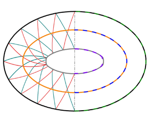
Hypersonic axisymmetric internal conical flow (ICF) usually serves as a basic model for internal compression systems including the inward-turning inlet (You, Zhu & Guo Reference You, Zhu and Guo2009; You Reference You2011; Zuo & Mölder Reference Zuo and Mölder2019), in which the inherent convergent effects of the shock wave have received extensive attention. It has been well documented that the internal conical shock (ICS) generated by the axisymmetric ring wedge (Ferri Reference Ferri1946; Mölder Reference Mölder1967; Mölder et al. Reference Mölder, Gulamhussein, Timofeev and Voinovich1997) will continuously strengthen until a Mach disk inevitably appears on the centreline (Rylov Reference Rylov1990; Ben-Dor Reference Ben-Dor2007; Isakova et al. Reference Isakova, Kraiko, Pyankov and Tillyayeva2012; Shoesmith et al. Reference Shoesmith, Mölder, Ogawa and Timofeev2017), causing serious total pressure loss and performance defects. From a practical point of view, intake flow is commonly non-axisymmetric. When the supersonic or hypersonic ICF deviates from the axisymmetric state either by the geometry (Mohan & Skews Reference Mohan and Skews2013; Zhang et al. Reference Zhang, Li, Ji, Si and Yang2021) or by the incoming flow (Ji et al. Reference Ji, Li, Zhang, Si and Yang2022), the convergent behaviours of the ICS fundamentally change and make the regular reflection possible on the centreline. Elliptical ring wedges proposed by Zhang et al. (Reference Zhang, Li, Ji, Si and Yang2021) are chosen as typical models in the hypersonic flow, in which the level of the deviation from the axial symmetry is quantified by the aspect ratio ( $AR$) between the major and minor axes. As shown in figure 1, the initial continuous and smooth ICS generated by the elliptical ring wedge gradually evolve into a complicated three-dimensional (3-D) morphology with kinks (Zhang et al. Reference Zhang, Li, Ji, Si and Yang2021). The kink is a typical singularity on the shock front, across which both the normal direction and the intensity of the shock front suffer finite jumps (Prasad Reference Prasad1995; Ben-Dor Reference Ben-Dor2007; Mostert et al. Reference Mostert, Pullin, Samtaney and Wheatley2017). It has been demonstrated that the emergence of kinks dampens the increment of the ICS strength and thus makes the regular reflection possible in the ICF (Zhang et al. Reference Zhang, Li, Ji, Si and Yang2021; Ji et al. Reference Ji, Li, Zhang, Si and Yang2022). The positions of kinks are of great importance in understanding the evolution and reflection of the ICS when the ICF deviates from the axisymmetric state. However, to the best of the authors’ knowledge, the theoretical prediction of kink formation in the ICF thus far remains limited because the complicated 3-D morphology of the ICS evolves.

Figure 1. (a) Schematic of the elliptical ring wedge and the ICS. (b) Numerical contours of normalized density on a typical cross-section of  $x/a=2.0$, where the free stream Mach number $M_\infty =6$, the entry aspect ratio $AR=1.43$, the leading-edge angle $\delta _0=10^\circ$ and the leading-edge radius along the major direction $a=100\ {\rm mm}$.
A low-cost and highly efficient way to analyse the evolution of the 3-D steady shock wave is using the method of spatial dimension reduction (Yang et al. Reference Yang, Teng, Jiang and Takayama2012; Xiang et al. Reference Xiang, Wang, Teng and Jiang2016) because the theory of two-dimensional (2-D) shock waves is well developed. To make the spatial dimension reduction available, the hypersonic equivalence principle (Anderson Reference Anderson2019; Wang Reference Wang2019) connecting the steady flow with the unsteady flow in one fewer space dimension can be adopted to equivalently transform the 3-D steady ICS into a 2-D moving shock with an initial elliptical shape. In other words, the evolution of the 3-D steady ICS is converted to the evolution of an equivalent 2-D elliptical moving shock (EMS). Since Whitham (Reference Whitham1957) first demonstrated the existence of kinks, the formation of kinks in various shock motions has been reported (Schwendeman Reference Schwendeman1988; Pullin et al. Reference Pullin, Mostert, Wheatley and Samtaney2014; Mostert et al. Reference Mostert, Pullin, Samtaney and Wheatley2016). For instance, Takayama, Kleine & Grönig (Reference Takayama, Kleine and Grönig1987) and Watanabe & Takayama (Reference Watanabe and Takayama1991) found that the disturbances generated by the experimental supports were amplified in the convergence of a cylindrical moving shock (CMS), which causes the formation of kinks on the shock front and thus makes the original CMS into a polygon. Apazidis (Reference Apazidis2003) theoretically and numerically illustrated the formation of kinks during the focusing of a strong shock in an elliptic cavity. When a planar shock was reflected on a wavy wall, the formation of kinks or triple points on the reflected shock was confirmed by both the experiments of Denet et al. (Reference Denet, Biamino, Lodato, Vervisch and Clavin2015) and the numerical simulations of Lodato, Vervisch & Clavin (Reference Lodato, Vervisch and Clavin2016, Reference Lodato, Vervisch and Clavin2017). The kinks indicate the distortion of the shock shape, which makes it difficult to theoretically analyse the shock evolution. Geometrical shock dynamics (GSD) (Han & Yin Reference Han and Yin1993; Whitham Reference Whitham2011) is a commonly used theory to examine the evolution of shock motions, in which the kink on the shock front is known as the ‘shock–shock’ (Prasad Reference Prasad1995; Mostert et al. Reference Mostert, Pullin, Samtaney and Wheatley2017). It is a high efficiency theory because it does not need to calculate the global downstream flow behind the shock (Whitham Reference Whitham2011). Therefore, the evolution of strong shocks such as converging shocks can be well predicted by GSD (Apazidis Reference Apazidis2003). With the help of GSD, Schwendeman (Reference Schwendeman1999) confirmed the formation of kinks during the collapse of a CMS when its initial Mach number is perturbed by a certain value, which ultimately makes the shock shape into straight segments (Schwendeman & Whitham Reference Schwendeman and Whitham1987). Subsequently, Mostert et al. (Reference Mostert, Pullin, Samtaney and Wheatley2018a,Reference Mostert, Pullin, Samtaney and Wheatleyb) found that the kink formation time is inversely proportional to the initial amplitude of the perturbation when assuming a sinusoidal distribution of the shock Mach numbers for an initially planar shock or CMS. As GSD is not formally derived from the Euler equations (Mostert et al. Reference Mostert, Pullin, Samtaney and Wheatley2018a) and neglects the non-uniform flow effects behind the shock (Han & Yin Reference Han and Yin1993; Shen et al. Reference Shen, Pullin, Samtaney and Wheatley2021), Best (Reference Best1991) pointed out that the accuracy of GSD is insufficient for weak shocks, in particular for blast shocks (Katko et al. Reference Katko, Chavez, Liu, Lawlor, McGuire, Zheng, Zanteson and Eliasson2020) or diverging shocks (Ridoux et al. Reference Ridoux, Lardjane, Monasse and Coulouvrat2018). For this scenario, a generalized GSD incorporating the non-uniformity of the flow immediately behind the shock was developed by Best (Reference Best1991, Reference Best1993), which can successfully yield a better solution compared with GSD (Katko et al. Reference Katko, Chavez, Liu, Lawlor, McGuire, Zheng, Zanteson and Eliasson2020). Recently, Shen et al. (Reference Shen, Pullin, Samtaney and Wheatley2021) used generalized GSD to analyse the evolution of a shock generated by an impulsively accelerated piston with a sinusoidal perturbation. They found that the kink formation time follows a scaling inversely proportional to the small perturbation amplitude, which is similar to the results reported by Mostert et al. (Reference Mostert, Pullin, Samtaney and Wheatley2018a). Compared with the generalized GSD, GSD reduce the calculation complexity and improve the computational efficiency although the accuracy of GSD is sacrificed to some extent for specific problems such as diverging shocks (Ridoux et al. Reference Ridoux, Lardjane, Monasse and Coulouvrat2018; Katko et al. Reference Katko, Chavez, Liu, Lawlor, McGuire, Zheng, Zanteson and Eliasson2020). Keep in mind that the present work focuses on the formation of kinks during the converging of an equivalent EMS, which can be solved by GSD with sufficient accuracy (Best Reference Best1991; Courant & Friedrichs Reference Courant and Friedrichs1999).
From the view of GSD, the deformation of the 2-D moving shock is generally accompanied by two families of characteristics that represent disturbances on the shock (Han & Yin Reference Han and Yin1993). It seems that the evolution of the 2-D moving shock with kinks can be solved by calculating the characteristics only. In practice, it is difficult to obtain the shock front because the time information is not involved in the characteristic relations (Akbar et al. Reference Akbar, Schwendeman, Shepherd, Williams and Thomas1995). To track the positions and shapes of the 2-D moving shock with time, the front tracking method (Henshaw, Smyth & Schwendeman Reference Henshaw, Smyth and Schwendeman1986; Schwendeman Reference Schwendeman1988) based on the kinematic equations of GSD was developed and applied to a variety of problems (Noumir et al. Reference Noumir, Le Guilcher, Lardjane, Monneau and Sarrazin2015; Qiu, Liu & Eliasson Reference Qiu, Liu and Eliasson2016; Ndebele, Skews & Paton Reference Ndebele, Skews and Paton2017; Ridoux et al. Reference Ridoux, Lardjane, Monasse and Coulouvrat2019). Unfortunately, the front tracking method does not take the characteristics (i.e. the propagation trajectories of the disturbances) into consideration, which is not conducive to revealing the mechanism of shock deformation. Therefore, simultaneously tracking the shape of the 2-D moving shock and the disturbances on the shock are of prime importance to understanding the evolution of the 3-D steady ICS from a 2-D unsteady perspective.
In this paper, a front-disturbance tracking method (FDTM) based on GSD is developed to simultaneously predict the evolution of a 2-D moving shock and reveal its deformation mechanisms. Combining the FDTM with the hypersonic equivalent principle, the convergent behaviours of the ICS generated by the elliptical ring wedges and the formation position and mechanism of kinks are investigated from the perspective of the equivalent 2-D moving shock. The remainder of this paper is organized as follows: the equivalent transformation of the 3-D steady ICS generated by the elliptical ring wedge into a 2-D moving shock is presented in § 2; the FDTM is developed in § 3; with the help of the FDTM, the convergent behaviours of the equivalent 2-D moving shock, the formation mechanism of the kinks and the effects of geometric parameters of the elliptical ring wedge on the position of kinks are discussed in § 4; and finally, conclusions are summarized in § 5.
2. Model and space dimensionality reduction
2.1. Description of the model
The schematic of the elliptical ring wedge in hypersonic flow with a free stream Mach number  $M_\infty$ is displayed in figure 1(a), where the leading-edge radii along the major and minor directions are denoted as $a$ and $b$, respectively. The leading-edge angle $\delta _0$ keeps the same value in the circumferential direction $\varphi$ to generate a convergent incident shock with a uniform strength on the leading-edge plane, where the circumferential angle $\varphi$ is defined as the angle from the $z$-axis to the polar line. The length of the elliptical ring wedge is $L$, which avoids the expansion waves generated from the trailing-edge of the wall affecting the elliptical ICS (Zhang et al. Reference Zhang, Li, Ji, Si and Yang2021). The origin $O$ of the coordinates is situated at the centre of the leading-edge plane, and the $x$,
$x$,  $y$ and $z$ axes denote the directions along the free stream, major and minor directions, respectively. Consequently, the inner wall profile of the elliptical ring wedge can be expressed as
 \begin{equation} \frac{y^2}{(a-x\tan\delta_0)^2}+\frac{z^2}{(b-x\tan\delta_0)^2}=1,\quad 0\leq x \leq L. \end{equation}
The independent dimensionless flow parameters are the free stream Mach number ( $M_\infty$) and specific heat ratio of the gas ( $\gamma$), which are fixed at $6$ and $1.4$ in the 3-D steady ICF, respectively. The independent dimensionless geometric parameters are $\delta _0$, the entry aspect ratio $AR=a/b$ and the length $L/a=1$, where $\delta _0$ and $a$ are fixed at $10^\circ$ and $100\ {\rm mm}$, respectively. It has been demonstrated that the kink formation positions and the reflection type of the ICSs are sensitive to $AR$ (Zhang et al. Reference Zhang, Li, Ji, Si and Yang2021). Therefore, $b$ varies to obtain different values of $AR$ on the leading-edge plane. Several typical elliptical ring wedges are listed in table 1. The effects of different $AR{\rm s}$ on the kink formation positions of the elliptical ICS are examined in § 4.3.
Table 1. Overview of several typical elliptical ring wedges.

2.2. Equivalent transformation of the ICS
The hypersonic equivalence principle (Anderson Reference Anderson2019) is a powerful theory built on the hypersonic small-disturbance equations for a calorically perfect gas in inviscid flow, which enables the 3-D steady flow to transform into a 2-D unsteady flow. As the free stream speed  $V_\infty$ is along the positive $x$ direction in the Cartesian coordinate system, the relationship between the coordinate $x$ in the 3-D steady flow and the time $t$ in the 2-D unsteady flow is connected by (Anderson Reference Anderson2019)
 \begin{equation} x=V_\infty t .\end{equation}
In other words, the lateral structure of the ICS at the  $x$ cross-section in the 3-D steady ICF is equivalent to the instantaneous structure of the moving shock at time $t$ in the 2-D unsteady flow.
As the shock strengthens along the  $x$ direction in the convergence process of the ICS, the speed change in the $x$ direction may no longer be a small amount compared with that in the flow cross-section. It seems that the applicability of the hypersonic equivalence principle decays along the $x$ direction in the ICF, especially near the convergence centre. Nevertheless, Zhang et al. (Reference Zhang, Li, Ji, Si and Yang2021) have shown that the appearance of kinks is far away from the convergence centre of the elliptical ring wedge to a certain extent. Thus, it is feasible to examine the formation of kinks using the hypersonic equivalence principle for spatial dimension reduction in this paper.
Figure 2 presents the equivalent schematic between the hypersonic 3-D steady ICF generated by the elliptical ring wedge and the 2-D unsteady flow. The ICS with the same shape as the entrance is generated at the leading-edge ( $x=0$) of the elliptical ring wedge, which converges downstream and shows the complicated 3-D surface. In the $y$–
$y$– $z$ plane, the evolution of the ICS can be equivalent to the convergence of a 2-D moving shock ( $S_0$) generated by a sudden contraction of an elliptical piston ( $W_0$) at time ( $t=0$), where the initial shapes of $S_0$ and $W_0$ are the same as the entrance of the elliptical ring wedge. As the elliptical piston contracts with a constant speed of $V_\infty \tan \delta _0$, the shape of the elliptical piston and the 2-D moving shock at time $t$ are equivalent to the inner wall profile of the elliptical ring wedge and the transverse structure of the 3-D ICS at $x=V_\infty t$, respectively. When the elliptical piston contracts to the same shape as the trailing-edge of the elliptical ring wedge ( $W_1$) at time $t_1=L/V_\infty$, the elliptical piston stops contracting, whereas the equivalent 2-D moving shock continues to converge towards the centre to yield the transverse structure of the 3-D ICS. In the above equivalence, obtaining the initial shock Mach number $M_{{s0}}$ of the equivalent 2-D moving shock is important. Once $M_{{s0}}$ is known, the equivalence can be performed.

Figure 2. Equivalent schematic between the 3-D steady ICF generated by the elliptical ring wedge (left) and the 2-D unsteady flow (right).
The equivalent shock intensity is obtained as follows. As the leading-edge angle  $\delta _0$ keeps the same value in the circumferential direction of the elliptical ring wedge, the shock angle $\lambda _0$ of the 3-D elliptical ICS at the leading-edge can be calculated by the oblique shock relationship as shown in (Zucrow & Hoffman Reference Zucrow and Hoffman1997)
 \begin{equation} \tan\delta_0=2\cot\lambda_0\frac{M_\infty^2\sin^2\lambda_0-1}{M_\infty^2[\gamma+ \cos( 2\lambda_0) ] +2}, \end{equation}
where  $\gamma =1.4$ is the specific heat ratio of the gas. According to the hypersonic equivalence principle, the circumferential distribution of the equivalent 2-D moving shock intensity is the same at time $t=0$, and $M_{{s0}}$ is given by
 \begin{equation} M_{{s0}}=M_\infty \tan\lambda_0. \end{equation}
 Substituting  $\delta _0=10^{\circ }$ and $M_\infty =6$ into (2.3) and (2.4) yields $M_{{s0}}=1.9$. Although $M_{{s0}}$ is the same in this paper, the initial shape of the equivalent 2-D moving shock varies with the $AR$ of the elliptical ring wedge, which presents different evolutions of the shock structures with time.
In summary, the spatial evolution of the complicated 3-D ICS generated by the elliptical ring wedges can be equivalent to the time evolution of the 2-D moving shock with an initial elliptical shape. After this equivalence, the convergent behaviours of the ICS and the formation of kinks can be analysed using GSD.
3. Front-disturbance tracking method
An FDTM based on GSD is developed to simultaneously track the equivalent 2-D moving shock front and the disturbances on the shock, which can be used to reveal the deformation mechanism of the shock and rapidly predict the evolution of the shock. The basic principles of the FDTM are introduced, based on which the procedure of the FDTM is described in detail. Finally, the FDTM is verified by the convergence of CMS with an initial uniform and non-uniform intensity.
3.1. Basic principles of the FDTM
The governing equations for tracking both the shock front and the propagation trajectory of the disturbances (i.e. the characteristics line) are the basic principles of the FDTM, which are presented as follows.
As shown in figure 3, the moving shock front is discretized by a series of points  $\boldsymbol {y}_i(t)$ in the Cartesian coordinate system ( $y,z$), where the subscript $i$ is the serial number of the discrete points. The perpendicular bisectors PQ and SR between adjacent discrete points represent rays, and $\theta$ is the angle between the ray and the positive $z$ direction. A small shock segment SP between adjacent rays at time $t$ moves and deforms to become segment RQ at time $t+{\rm \Delta} t$. The main assumption in GSD is that each shock segment propagates down a tube whose boundaries are defined by the rays. In other words, the motion of the shock only changes with the variation of the ray tube area. Thus, the motion of the shock can be predicted by the relation between the moving shock Mach number ( $M_{{s}}$) and the ray tube area ( $A$) (Chester Reference Chester1954; Chisnell Reference Chisnell1957; Whitham Reference Whitham1957, Reference Whitham1958), which can be expressed as
 \begin{equation} \frac{2M_{{s}}\mathrm{d}M_{{s}}}{(M_{{s}}^2-1)K(M_{{s}})}={-}\frac{\mathrm{d}A}{A}, \end{equation}
where
 $$\begin{gather} K(M_{{s}})={2}{\left(2\mu+1+\frac{1}{M_{{s}}^2}\right)^{{-}1} \left(1+\frac{2}{\gamma+1}\frac{1-\mu^2}{\mu}\right)^{{-}1}}, \end{gather}$$
 $$\begin{gather}\mu=\left[{\frac{(\gamma-1)M_{{s}}^2+2}{2\gamma M_{{s}}^2-(\gamma-1)}}\right]^{{-}1}. \end{gather}$$
Let  $\boldsymbol {y}_i(t)$, $M_{{{s}}i} (t)$ and $\boldsymbol {n}_i(t)$ represent the position vector, the moving shock Mach number and the unit normal vector at the small shock segment, respectively; then, the motion of the shock in the ray tube satisfies
 \begin{equation} \frac{\mathrm{d}}{\mathrm{d}t}\boldsymbol{y}_i(t)=c_0M_{{{s}}i} (t)\boldsymbol{n}_i(t),\quad i=1,2,\ldots,N, \end{equation}
where  $N$ is the total number of discrete points at time $t$, and $c_0$ is the speed of sound ahead of the moving shock. The ray angle $\theta _i$ at the small shock segment is
 \begin{equation} \tan \theta_i =\frac{n_{yi}}{n_{zi}},\quad i=1,2,\ldots,N, \end{equation}
where  $n_{yi}$ and $n_{zi}$ are the components of the unit normal vector $\boldsymbol {n}_i$ in the $y$ and $z$ directions, respectively. Equations (3.1) and (3.4) are the kinematic equations governing the motion of the shock in the FDTM, which can be used to quickly predict the evolution of the moving shock.

Figure 3. Shock positions at time  $t$ and $t+{\rm \Delta} t$ (solid lines) and rays (dashed lines) in Cartesian coordinate system ( $y,z$).
The shock deformation mechanism cannot be revealed by only solving (3.1) and (3.4) because the disturbances propagating on the shock front that cause the shock deformations are not considered. From the perspective of GSD, when the small shock segment propagates in the ray tube, the shock segment sends out disturbance waves at the foot where the shock wave contacts the ray. Since the normal vector at each discrete point (i.e. the grey solid lines with arrows in figure 3) is also a ray, the disturbances propagating on the shock front can be regarded as emanating from the discrete point, which changes the strength and shape of the moving shock. The disturbances that intensify and weaken the moving shock are the so-called shock–compression and shock–expansion in GSD, respectively (Whitham Reference Whitham1957, Reference Whitham1958), while the disturbance that makes the shock front discontinuous is the so-called shock–shock disturbance (Han & Yin Reference Han and Yin1993; Xie, Han & Takayama Reference Xie, Han and Takayama2005). The propagation trajectories of the disturbances are represented by two families of characteristics in GSD. Therefore, it is necessary to solve the characteristics while the shock front is advancing in the FDTM. The characteristic equations derived by Whitham (Reference Whitham1957, Reference Whitham1958) are provided in the Cartesian coordinate system as
 $$\begin{gather} \frac{\mathrm{d}y}{\mathrm{d}z}=\tan(\theta_i+\nu_i), \end{gather}$$
 $$\begin{gather}\frac{\mathrm{d}y}{\mathrm{d}z}=\tan(\theta_i-\nu_i), \end{gather}$$
where  $\nu _i$ is the included angle between the characteristic and the ray, which can be written as (Han & Yin Reference Han and Yin1993)
 \begin{equation} \tan \nu_i = \frac{1}{M_{{{s}}i}}\left[ {\frac{1}{2}(M_{{{s}}i}^2-1)K(M_{{{s}}i})}\right] ^{1/2}. \end{equation}
To distinguish the propagation directions of the disturbances, standing on the shock front and facing the direction of the shock motion, the disturbances propagating to the left and right are named characteristics  $C^+$ and $C^-$, respectively (Han & Yin Reference Han and Yin1993). The characteristic equations (3.6) and (3.7) are used to track the characteristics $C^+$ and $C^-$ in the FDTM, respectively.
Since  $M_{{{s}}i}$ in (3.8) is the same as that in (3.4), the characteristic equations for tracking the propagation trajectory of the disturbances are spontaneously integrated into the kinematic governing equations for tracking the shock front. However, a close combination of the shock front and the characteristics is still needed to simultaneously track the shock front and the disturbances in the FDTM.
Figure 4 illustrates the schematic of the FDTM. The initial shape and intensity of the shock front at time  $t_0$ are given in advance, which is discretized by a series of points. These discrete points on the initial shock front are also the starting points of characteristics $C^+$ and $C^-$. In other words, these discrete points have dual identities on the initial shock front. With time-marching, the moving shock front at any subsequent time $t$ consists of a new series of points, which come from two sources. One set of points comes from the shock front itself that is advancing in each ray tube governed by (3.1) and (3.4). The others come from the characteristics $C^+$ and $C^-$ emanating from the discrete points on the initial shock front that intersects with the shock front governed by the characteristic equations (3.6) or (3.7). Harmonizing the discrete points on the shock front coming from the two sources is of prime importance in the FDTM. To guarantee that the characteristics can be traced back to the discrete points of the initial shock front, the intersections between the characteristics and the shock front are retained for the next time step. In other words, these intersections on the shock front have dual identities in the FDTM to simultaneously track the shock front and the disturbances at any subsequent time. The detailed procedure of the FDTM is given in § 3.2.

Figure 4. Schematic of a FDTM.
3.2. Procedure of the FDTM
The time-marching procedure of the FDTM is described in detail between adjacent times  $t$ and $t+{\rm \Delta} t$ here, where the time step, ${\rm \Delta} t$, is restricted by the stability condition of the algorithm (De Moura & Kubrusly Reference De Moura and Kubrusly2013) and the non-cross-condition of rays (Henshaw et al. Reference Henshaw, Smyth and Schwendeman1986; Ridoux et al. Reference Ridoux, Lardjane, Monasse and Coulouvrat2019). As shown in figure 4, the shock front at time $t$ is discretized by points $\boldsymbol {y}_i(t)$ with shock Mach numbers $M_{{{s}}i} (t)$, ray angles $\theta _i (t)$ and included angles $\nu _i (t)$. The grey solid lines with arrows between the shock front at times $t$ and $t+{\rm \Delta} t$ represent the normal directions of the shock front at points $\boldsymbol {y}_i(t)$, which can be expressed by the unit normal vector $\boldsymbol {n}_i(t)$. The perpendicular bisectors between adjacent discrete points at time $t$ represent rays (i.e. the grey dashed lines). At adjacent time steps, the FDTM can be mainly divided into three procedures: the front tracking module; the disturbance tracking module; and the redistribution module with a termination criterion.
The flowchart of the front tracking module is shown in the Appendix. As the discrete points  $\boldsymbol {y}_i(t)$ on the shock front, the moving shock Mach numbers $M_{{{s}}i} (t)$ and the unit normal vectors $\boldsymbol {n}_i(t)$ are known at time $t$, and the shock front can be advanced along $\boldsymbol {n}_i(t)$ using a third-order Runge–Kutta scheme (Gottlieb & Shu Reference Gottlieb and Shu1998) to solve (3.4). As a result, the front tracking points $\boldsymbol {y}_i(t+{\rm \Delta} t)$ on the shock front at time $t+{\rm \Delta} t$ are determined (see the blue hollow points in figure 4). After this step, the ray tube areas $A_i (t)$ and $A_i (t+{\rm \Delta} t)$ (i.e. the length of each shock segment in the ray tube) can be calculated using the positions of $\boldsymbol {y}_i(t)$ and $\boldsymbol {y}_i(t+{\rm \Delta} t)$ (Henshaw et al. Reference Henshaw, Smyth and Schwendeman1986; Ridoux et al. Reference Ridoux, Lardjane, Monasse and Coulouvrat2019), respectively. Integrating (3.1) on each ray tube, the moving shock Mach number $M_{{{s}}i} (t+{\rm \Delta} t)$ at the front tracking points $\boldsymbol {y}_i(t+{\rm \Delta} t)$ can be obtained. In short, the procedure of the front tracking module in the FDTM can calculate the shock shape and its intensity at time $t+{\rm \Delta} t$ by solving (3.1) and (3.4).
When the shock front moves from time  $t$ to $t+{\rm \Delta} t$, the disturbances synchronously propagate along the shock front. The flowchart of the disturbances tracking module is given in the Appendix. As the discrete points $\boldsymbol {y}_i(t)$, the shock Mach number $M_{{{s}}i} (t)$, the ray angle $\theta _i (t)$ and the included angle $\nu _i (t)$ are all known in the previous front tracking module, the intersections between the characteristics and the shock front at the time $t+{\rm \Delta} t$ are solved by combining the shock front at time $t+{\rm \Delta} t$ with (3.6) or (3.7). Thus, the disturbance tracking points $\boldsymbol {Y}_j(t+{\rm \Delta} t)$ on the shock front yield at time $t+{\rm \Delta} t$, where the subscript $j$ is the serial number of the characteristics. Note that all these disturbance tracking points can be traced back to the discrete points on the initial shock front. The moving shock Mach numbers $M_{{{s}}j} (t+{\rm \Delta} t)$ on these disturbance tracking points $\boldsymbol {Y}_j(t+{\rm \Delta} t)$ are determined by linear interpolation among the already known $M_{{{s}}i} (t+{\rm \Delta} t)$. In short, the procedure of the disturbance tracking module in the FDTM can track the characteristics $C^+$ and $C^-$ on the shock front at time $t+{\rm \Delta} t$ by solving (3.6) and (3.7).
After the above two modules in the FDTM are completed, the flowchart of the redistribution module with a termination criterion can be performed, which is shown in the Appendix. Since the disturbance tracking points  $\boldsymbol {Y}_j(t+{\rm \Delta} t)$ inherit all information on the moving shock front, they are retained as the new discrete points on the shock front at time $t+{\rm \Delta} t$, whereas the front tracking points $\boldsymbol {y}_i(t+{\rm \Delta} t)$ calculated by the previous front tracking module are deleted. These new discrete points on the shock front are renumbered $\boldsymbol {y}_i(t+{\rm \Delta} t)$ for the next time step, each of which has dual identities to simultaneously track the shock front and the disturbances. In other words, the discrete points on the shock front from two sources during each time step are harmonized in the FDTM, which improves the calculation efficiency. Following the procedure used by Ridoux et al. (Reference Ridoux, Lardjane, Monasse and Coulouvrat2019), an interpolation of the shock front is performed using a monotone cubic method (Huynh Reference Huynh1993) to determine the unit normal vectors $\boldsymbol {n}_i(t+{\rm \Delta} t)$ at the new discrete points $\boldsymbol {y}_i(t+{\rm \Delta} t)$ at time $t+{\rm \Delta} t$. Moreover, the angles $\theta _i (t+{\rm \Delta} t)$ and $\nu _i (t+{\rm \Delta} t)$ at the new discrete points are calculated by (3.5) and (3.8) using the unit normal vectors $\boldsymbol {n}_i(t+{\rm \Delta} t)$ and the shock Mach numbers $M_{{{s}}i} (t+{\rm \Delta} t)$. Thus, all the information for shock advancing in the next time step is known on the new discrete points on the shock front. Before the shock advances, a termination criterion is examined. When the same family of adjacent characteristics $C^+$ or $C^-$ intersect, the shock–compression disturbances transform into a shock–shock disturbance and thus, the kink forms. Taking the intersection of two adjacent characteristics $C^-$ as an example, figure 5 gives the schematic of the numerical procedure for determining the kink formation on the shock front. As shown in figure 5, the two adjacent characteristics $C^-$ intersect at a point E between time $t$ and $t+{\rm \Delta} t$, which means that the last time step should be shortened from ${\rm \Delta} t$ to ${\rm \Delta} t^{\prime }$ for the kink formation. To quickly evaluate ${\rm \Delta} t^{\prime }$, one can find a point D on the shock front at time $t$, which yields the shortest distance $l$ between D and E. Then, ${\rm \Delta} t^{\prime }=l/({M_{{sD}}} c_0)$, where $M_{{sD}}$ is the moving shock Mach number at point D. Since $M_{{sD}}$ can be calculated by linear interpolation along the shock front at time $t$,
$t$,  ${\rm \Delta} t^{\prime }$ is obtained. Thus, the shock front and characteristics at time $t+{\rm \Delta} t^{\prime }$ can be calculated by the front tracking module and the disturbance tracking module from time $t$, respectively. As the kink (i.e. E in figure 5) forms on the shock front at time $t+{\rm \Delta} t^{\prime }$, the shock advancing is terminated in the FDTM. Otherwise, the discrete points with dual identities on the shock front at time $t+{\rm \Delta} t$ continue to advance until the termination criterion is satisfied. Note that the formation of the kink on the shock front does not mean the end of the shock converging. The kink is not a stable shock anchoring, but a triple point moving with the shock evolution.

Figure 5. Schematic of the numerical procedure for determining the kink formation on the shock front.
From the above three modules, one can construct an entire flowchart of the FDTM in the Appendix. Once the initial shape and intensity distribution of the moving shock are given, the evolution of the moving shock and the disturbances causing the shock deformation can be simultaneously tracked.
3.3. Verification of the FDTM
3.3.1. Convergence of a CMS with initial uniform intensity
The convergence of a CMS is selected as a typical case to validate the FDTM, which can be equivalent to the axisymmetric ICS generated by a ring wedge (i.e.  $AR = 1.0$) in the present study. On the one hand, this typical case is a baseline that can be compared with the EMSs in § 4. On the other hand, much theoretical and experimental research on the convergence of the CMS has been performed (Guderley Reference Guderley1942; Takayama et al. Reference Takayama, Kleine and Grönig1987; Hornung, Pullin & Ponchaut Reference Hornung, Pullin and Ponchaut2008); thus, the accuracy of the FDTM can be validated by the theoretical evolution of the cylindrical shock front (Hornung et al. Reference Hornung, Pullin and Ponchaut2008) and the theoretical characteristics in GSD (Han & Yin Reference Han and Yin1993). The initial radius of the CMS is $R_0=a$, and the initial moving shock Mach number is $M_{{s0}}=1.9$, which is equivalent to the axisymmetric ICS generated by a ring wedge with $\delta _0=10^{\circ }$ in $M_\infty =6$.
The initial shock front is discretized circumferentially with an equal length in the FDTM. Three sets of initial lengths with  ${\rm \Delta} s_0/S_0=5\times 10^{-3}$, ${\rm \Delta} s_0/S_0=2.5\times 10^{-3}$ and ${\rm \Delta} s_0/S_0=1.25\times 10^{-3}$ are tested, corresponding to the initial discrete point numbers of 200, 400 and 800, where ${\rm \Delta} s_0$ and $S_0$ are the length of the shock segment in the ray tube and the circumference of the cylindrical shock itself at initial time $t=0$, respectively. Although the CMS can converge to the centre, the convergence of the axisymmetric ICS is terminated early by the Mach disk before the converging centre (Zhang et al. Reference Zhang, Li, Ji, Si and Yang2021). To keep the equivalence between the CMS and the axisymmetric ICS, the convergence termination of the CMS in the FDTM is set as $t/T=2.62$ with $T=a/V_\infty$, which corresponds to the position of the Mach disk at $x/a=2.62$ in the axisymmetric ICS (Zhang et al. Reference Zhang, Li, Ji, Si and Yang2021; Ji et al. Reference Ji, Li, Zhang, Si and Yang2022).
As shown in figure 6(a), the variations in the shock front radius ( $R$) with time $t$ calculated by the FDTM with three sets of discrete points are compared with the theoretical solution reported by Hornung et al. (Reference Hornung, Pullin and Ponchaut2008) who used the integral form of the relation (3.1) to obtain the theoretical evolution of the CMS. The horizontal and vertical coordinates in figure 6(a) maintain the scale of $1:1$ to illustrate the real shape of the shock front. To highlight the differences between the FDTM and the theoretical solution, figure 6(b) gives the relative errors ${\rm \Delta} R/R_{{T}}$, where ${\rm \Delta} R=R_{{T}}-R_{{F}}$, $R_{{T}}$ and $R_{{F}}$ are the shock radii calculated by the theory and the FDTM, respectively. The shock front calculated by the FDTM essentially agrees with the theoretical solution. When the initial discrete points on the shock front with a spatial resolution of ${\rm \Delta} s_0/S_0=2.5\times 10^{-3}$, the evolution of the CMS can be accurately calculated by the FDTM with a relative error less than $4\,\%$. Therefore, the initial length of ${\rm \Delta} s_0/S_0=2.5\times 10^{-3}$ is used for all cases in the present study. To examine the characteristics calculated by the FDTM, any characteristic $C^+$ or $C^-$ can be used because the flow is axisymmetric. The characteristic $C^+$ originating from the endpoint of the initial shock front on the negative $z$-axis is shown in figure 6(c), which is compared with the theoretical characteristic solution solved directly using the characteristic relations. Similarly, figure 6(d) gives the relative errors ${\rm \Delta} y/y_{{T}}$ between the characteristic $C^+$ calculated by the FDTM and the theoretical solution, where ${\rm \Delta} y =y_{{T}}-y_{{F}}$, $y_{{T}}$ and $y_{{F}}$ are the ordinates calculated by the theory and the FDTM, respectively. Good agreement with a relative error less than $3\,\%$ is achieved in the shape of the characteristic when ${\rm \Delta} s_0/S_0=2.5\times 10^{-3}$. However, the time information is not contained in the theoretical characteristic solution, which cannot match the evolution of the shock front. Fortunately, the FDTM in the present study break through this limitation, which combines the evolution of the shock front with the disturbances on the shock front in real time. With the help of the FDTM, the evolution of the CMS can be further analysed as follows.

Figure 6. (a) Theoretical solution of the shock front radius ( $R$) varying with time t and the results calculated by the FDTM with three sets of discrete points. (b) Relative errors ${\rm \Delta} R/R_{{T}}$ between the theoretical shock radii and those calculated by the FDTM. (c) Characteristic $C^+$ originating from the endpoint of the initial shock front on the negative $z$-axis calculated by the FDTM and the theoretical solution. (d) Relative errors ${\rm \Delta} y/y_{{T}}$ between the characteristic $C^+$ calculated by the FDTM and the theoretical solution for $M_\infty =6$, $AR=1.0$ and $\delta _0=10^\circ$.
Figure 7 shows the instantaneous shock fronts at typical times of  $t/T=0, 1.31$ and 2.62, on which a set of characteristics $C^+$ and $C^-$ in every 20 points are superimposed. All results are calculated by the FDTM with ${\rm \Delta} s_0/S_0=2.5\times 10^{-3}$. The initial CMS accompanies bidirectional disturbances, which propagate along the shock front during convergence to intensify the shock. Hence, those disturbances are shock–compression. Note that the intervals between any adjacent disturbances from the same family are equal in real time. In other words, those disturbances can be regarded as uniform disturbances, which guarantee that the CMS always maintains a circular shape. In short, the evolution of the CMS is equivalent to that of the axisymmetric ICS before the formation of the Mach disk.

Figure 7. Shock front at the time  $t/T=0, 1.31$ and 2.62, characteristics $C^+$ and $C^-$ calculated by the FDTM with ${\rm \Delta} s_0/S_0=2.5\times 10^{-3}$ for $M_\infty =6$, $AR=1.0$ and $\delta _0=10^\circ$.
3.3.2. Convergence of the CMS with initial non-uniform intensity
As shown in § 3.3.1, when the initial shock Mach numbers along the CMS are the same, the converging shock always maintains a circular shape. However, the CMS is unstable to small disturbances (Whitham Reference Whitham1957). When the initial shock Mach number of the CMS is perturbed by a small value, the disturbances increase with the converging shock and thus, kinks appear and make the shock shape into straight segments (Schwendeman Reference Schwendeman1999). Similar behaviours were also observed in experiments (Takayama et al. Reference Takayama, Kleine and Grönig1987; Watanabe & Takayama Reference Watanabe and Takayama1991). To examine the accuracy of the FDTM in predicting the formation time and position of kinks, the evolution of a converging CMS with an initial perturbation in its intensity is adopted for validation. Since this specific case was numerically solved using GSD by Schwendeman (Reference Schwendeman1993, Reference Schwendeman1999), the same description of the problem is used here.
The initial shape of the CMS in the Cartesian coordinate system  $(x,y)$ is
 \begin{equation} x={\rm e}^{{-}r}\cos\left( 2 {\rm \pi}s\right),\quad y={\rm e}^{{-}r}\sin\left( 2 {\rm \pi}s\right), \end{equation}
where the initial radial distance  $R_0={\rm e}^{-r}$ with $r=0$, and $s\in [0,1)$. The initial distribution of the shock Mach number $M_{{s0}}$ along the CMS is
 \begin{equation} M_{{s0}}=2+0.2\sin(10 {\rm \pi}s). \end{equation}
In the perspective of GSD, the disturbances induced by the initial non-uniformity in the shock intensities gradually increase and aggregate during the CMS convergence, which causes the shock shape to deviate from the circular shape and form kinks on the shock front.
Figure 8(a) shows the shock fronts calculated by the FDTM at typical time  $T_n=0,0.32$ and $1.05$ with ${\rm \Delta} s_0 / S_0 =2.5 \times 10^{-3}$, on which a set of characteristics $C^+$ and $C^-$ in every $20$ points are superimposed and anticlockwise numbered as $1,2,\ldots,j$. With the help of FDTM, the evolution of the converging shock can be further analysed. The bidirectional shock–compression disturbances caused by the initial non-uniformity of the shock intensity unevenly propagate along the shock front (i.e. the characteristics), which plays a prominent role for the deformation and non-uniform intensification of the shock. As the shock converges, the interval between any adjacent shock–compression disturbances from the same family continuously decreases (see figure 8a). When the shock–compression disturbances from the same family intersect, the shock–compression disturbances transit to the shock–shock disturbance (Han & Yin Reference Han and Yin1993), which indicates the kink formation. Due to the five-fold circular symmetry of the initial perturbation in (3.10), five pairs of left-running and right-running shock–shocks (i.e. 10 kinks) on the converging shock front are formed simultaneously, which divides the converging shock front into 10 shock segments at $T_n=1.05$. Specifically, the intersection point between the characteristics $C_1^-$ and $C_2^-$ in the enlarged view of figure 8(a) is $(x/R_0,y/R_0)=(0.2131,-0.2346)$, which is the formation position of the kink. The shock fronts calculated by Schwendeman (Reference Schwendeman1999) are also superimposed on figure 8(a), where the formation position of the kink is $(x/R_0,y/R_0)=(0.2130,-0.2345)$. Thus, the relative error of the kink formation positions is less than $0.1\,\%$. Furthermore, when the converging shock front passes the circle with a radius of ${\rm e}^{-r}$ and $r = 0.5$ (i.e. the grey dotted line in figure 8a before the kink formation), Schwendeman (Reference Schwendeman1999) provided the shock Mach numbers. These shock Mach numbers are compared with those calculated by the FDTM in figure 8(b), which yields a relative error less than $3\,\%$ at the peak and trough positions. Thus, the FDTM can well predict the evolution of the converging CMS with an initial non-uniformity in its intensity.

Figure 8. (a) Evolution of the shock front and characteristics. (b) Comparison of shock Mach numbers when the shock passes the circle with a radius of  ${\rm e}^{-r}$ and $r = 0.5$.
For the converging CMS with a large  $M_{{s0}}$ and a sufficiently small perturbation, an asymptotic solution for the kink formation time $T_{{K}}$ and the corresponding shock radius $R_{{K}}$ was derived by Mostert et al. (Reference Mostert, Pullin, Samtaney and Wheatley2018b), which is adopted here to further illustrate the performance of the FDTM. The initial shape of the CMS satisfies (3.9a,b), while the initial distribution of the shock Mach numbers is consistent with that of Mostert et al. (Reference Mostert, Pullin, Samtaney and Wheatley2018b), which can be expressed as
 $$\begin{gather} M_{{s0}}=20[ 1 +q \epsilon \sin( 2 {\rm \pi}qs)]^{{-}1/n}, \end{gather}$$
 $$\begin{gather}n=1+\frac{2}{\gamma}+\left( \frac{2 \gamma}{\gamma-1}\right)^{1/2}, \end{gather}$$
where  $2{\rm \pi} /q$ is periodic over CMS with a wavenumber $q=8$, and $\epsilon$ is a perturbation amplitude, and $\gamma =5/3$. The cases with $q^2\epsilon =0.16,0.32,0.64,0.96,1.28$ and $1.6$ are calculated by the FDTM, and the corresponding formation time of the kinks are extracted for comparisons with the literature.
The kink formation time  $T_{{K}}$ and the corresponding shock radius $R_{{K}}$ calculated by the FDTM are shown in figures 9(a) and 9(b), respectively, where the abscissa and ordinate are displayed in logarithms. The asymptotic solution reported by Mostert et al. (Reference Mostert, Pullin, Samtaney and Wheatley2018a,Reference Mostert, Pullin, Samtaney and Wheatleyb) using the nonlinear Fourier-based analysis method, and the numerical results obtained by the method of Schwendeman (Reference Schwendeman1993) using GSD are superimposed on figure 9. It is obvious that $T_{{K}}$ and $R_{{K}}$ calculated by the FDTM agree well with the numerical results reported by Schwendeman (Reference Schwendeman1993). Both of them approach the asymptotic solution as $q^2 \epsilon$ decreases. In other words, the formation of a kink in the limit $q^2 \epsilon \longrightarrow 0$ is suggested by the asymptotic solution, which is in support of the results calculated by the FDTM.

Figure 9. (a) Comparisons of the kink formation time  $T_{{K}}$ for $M_{{s0}}=20$, $q=8$ and $\gamma =5/3$. (b) Comparisons of shock radius $R_{{K}}$ at the kink formation for $M_{{s0}}=20$, $q=8$ and $\gamma =5/3$.
In short, the collapse of a CMS with an initial non-uniformity in its intensity can be solved by the FDTM with sufficient accuracy. Undoubtedly, once the converging CMS deviates from the axisymmetric state to be an EMS that is equivalent to an elliptical ICS, kinks also appear on the shock front. With the help of FDTM, it is valuable to address the evolution mechanisms of the elliptical ICS, which is discussed in § 4.
4. Kinks on elliptical convergent shock waves in the ICFs
Combining the FDTM with the hypersonic equivalent principle, the convergent behaviours of the 3-D elliptical ICS and the formation mechanism of kinks are investigated from the perspective of the equivalent 2-D moving shock, in which the effects of different  $AR{\rm s}$ on the kinks are discussed.
4.1. Range of kink emergence prior to the Mach disk
The convergent behaviours of the elliptical ICS from the leading-edge of the elliptical ring wedge to a location where the kink forms are considered in the present study. This evolution stage is far from the convergence centre, and thus, the hypersonic equivalence principle works. However, if the ICS slightly deviates from the axisymmetric state, the elliptical ICS may form a Mach disk early to prevent the appearance of kinks (Zhang et al. Reference Zhang, Li, Ji, Si and Yang2021). Due to the complicated 3-D flow, the exact position of the Mach disk in the ICS is so far difficult to theoretically determine. To predict the formation of kinks on the elliptical ICS using the FDTM, it is therefore of paramount importance to make sure that kinks appear prior to the Mach disk.
In practice, the shock intensity is an important factor that affects the Mach disk (Tan, Ren & Wu Reference Tan, Ren and Wu2006; Guan et al. Reference Guan, Bai, Lin and Wu2020). It is well known that the shock intensity in the major plane of the elliptical ICS is always the largest during the convergence of an elliptical ICS (Zhang et al. Reference Zhang, Li, Ji, Si and Yang2021). If the shock angle  $\lambda _{{M}}$ in the major plane of the elliptical ICS is smaller than the shock angle $\lambda _{{N}}$ specified by the von Neumann (Reference von Neumann1943) criterion, the Mach disk does not appear in this flow cross-section. In other words, $\lambda _{{M}}=\lambda _{{N}}$ can be used as a conservative criterion to limit the position of the Mach disk. Thus, the FDTM can at least be used to predict the formation of kinks on the elliptical ICS where $\lambda _{{M}}< \lambda _{{N}}$. This criterion is performed as follows. When kinks appear on the equivalent 2-D EMS, the shock Mach number $M_{{sM}}$ at the $y$-axis (i.e. the major axis) is already obtained using the FDTM. Thus, the equivalent shock angle $\lambda _{{M}}$ in the major plane of the 3-D elliptical ICS can be calculated by the conversion relation
 \begin{equation} \tan \lambda_{{M}} =\frac{M_{{sM}}}{M_\infty}. \end{equation}
If  $\lambda _{{M}} < \lambda _{{N}}$, kinks appear prior to the Mach disk, which can be equivalent to the evolution of the elliptical ICS; otherwise, the appearance of kinks on the elliptical ICS cannot be guaranteed.
Figure 10 shows the von Neumann line ( $\lambda _{{M}} = \lambda _{{N}}$) of the elliptical ring wedges in the range of $AR=1.0$ to $5.0$ and $\delta _0=6^{\circ }$ to $14^{\circ }$ in $M_\infty =6$, which yields the conservative area for kinks appearing prior to the Mach disk. When $AR$ maintains the same value, the shock angle $\lambda _{{M}}$ can reach $\lambda _{{N}}$ with increasing $\delta _0$. However, under the premise of constant $\delta _0$, when $AR$ is sufficiently large, $\lambda _{{M}}$ cannot reach $\lambda _{{N}}$. The convergent behaviours of the elliptical ICS and the formation mechanism of kinks are discussed within the conservative area ( $\lambda _{{M}} < \lambda _{{N}}$) shown in figure 10.

Figure 10. The von Neumann line ( $\lambda _{{M}} = \lambda _{{N}}$) of the elliptical ring wedges in the range of $AR=1.0$ to $5.0$ and $\delta _0=6^{\circ }$ to $14^{\circ }$ in $M_\infty =6$.
4.2. Convergent behaviours and the formation mechanism of kinks
Experimental and numerical studies on the 3-D elliptical ICS (Zhang et al. Reference Zhang, Li, Ji, Si and Yang2021) demonstrated that the evolutions of different elliptical ICSs from an initially elliptical shape to a complex morphology with kinks are similar in general convergent behaviours. Taking  $AR=1.43$ and $\delta _0=10^{\circ }$ in $M_\infty =6$ as a typical example (see table 1) demonstrates the convergent behaviours of the elliptical ICS, which has been well documented by Zhang et al. (Reference Zhang, Li, Ji, Si and Yang2021) using 3-D numerical simulation. Thus, the convergent behaviours of the typical elliptical ICS can be compared with those calculated by the present FDTM from the equivalent 2-D unsteady perspective, in which the formation mechanism of kinks is also revealed using the FDTM.
4.2.1. Convergent behaviours of the equivalent EMS
The convergent behaviours of the equivalent EMS are calculated by the FDTM with  ${\rm \Delta} s_0/S_0=2.5\times 10^{-3}$, in which the propagation trajectories of the disturbances (i.e. characteristics $C^+$ and $C^-$) emitted from the initial shock front are tracked in real time. The instantaneous shock fronts at typical times of $t/T=0, 0.798$ and 1.596 are shown in figure 11(a), on which a set of characteristics $C^+$ and $C^-$ in the upper half-plane every 20 points are superimposed and anticlockwise numbered as $0,1,\ldots,j$ from the positive $z$-axis. When the shock converges to time $t/T=1.596$, the termination criterion of the calculation in the FDTM is met, which indicates that the characteristics in the same family intersect to form kinks. Due to the geometric symmetry, four kinks concurrently appear on the shock front at ( $y/a,z/a)=(\pm 0.396,\pm 0.047)$, which divide the shock front into two pairs of arch-shaped shock segments.

Figure 11. (a) Evolution of the shock front and characteristics, where dashed lines are the results of Computational Fluid Dynamics (CFD). (b) Circumferential distribution of the pressure ratio in the evolution of the shock for  $AR=1.43$ when $\delta _0=10^{\circ }$ and $M_\infty =6$, where solid points are the results of Computational Fluid Dynamics (CFD).
For comparison, a 3-D Euler solver based on the finite volume method was employed to simulate the 3-D steady elliptical flow field, in which the effects of viscosity and the presence of a boundary layer on the shock front were deemed negligible (Zhang et al. Reference Zhang, Li, Ji, Si and Yang2021). The computational domain, boundary conditions, numerical schemes, etc., adopted for all 3-D validation cases in this paper are consistent with the numerical simulations conducted by Zhang et al. (Reference Zhang, Li, Ji, Si and Yang2021). In short, this solver has been demonstrated reliable in our previous studies (Zhang et al. Reference Zhang, Li, Ji, Si and Yang2021; Ji et al. Reference Ji, Li, Zhang, Si and Yang2022), in which it captured complex shock structures well. The equivalent shock fronts on  $x/a=0, 0.798$ and 1.596 are extracted from the 3-D numerical simulation (Zhang et al. Reference Zhang, Li, Ji, Si and Yang2021) and superimposed on the lower half-plane in figure 11(a), where the formation positions of kinks are ( $y/a,z/a)=(\pm 0.387,\pm 0.050)$. As the relative difference in the kink positions between the FDTM and the 3-D numerical simulation is less than $6\,\%$, the evolution of the shock fronts calculated by the FDTM essentially agrees with the previous 3-D numerical simulation under the premise of equivalence. It must be emphasized that the FDTM can rapidly and quantitatively determine the evolution of the shock fronts and the formation positions of kinks with significantly lower cost than the 3-D numerical simulation. Moreover, figure 11(b) compares the circumferential distributions of the pressure ratio ( $p/p_\infty$) across the shock (i.e. the shock intensity) calculated by the FDTM and the 3-D numerical simulation, where the shock intensity distributions of the equivalent EMS are calculated by the oblique shock relationship,
 \begin{equation} \frac{p}{p_\infty}=1+\frac{2\gamma}{\gamma+1}\left\lbrace M_\infty^2\sin^2 \left[\arctan\left( \frac{M_{{s}}}{M_\infty} \right)\right] -1\right\rbrace, \end{equation}
where  $p_\infty$ is the pressure ahead of the shock. As shown in figure 11(b), the shock intensities calculated by the FDTM are also in good agreement with those of the 3-D numerical simulation. Although the initial elliptical shock has a circumferentially uniform intensity, the shock intensities near the major axis ( $\varphi = 90^{\circ },270^{\circ }$) significantly increase with shock convergence. As a result, kinks are formed near the major axis, which not only indicate the discontinuity of the shock front but also indicate a sharp change in the shock intensity. With the help of the FDTM, the evolution of the EMS can be further analysed. As shown in the upper half-plane in figure 11(a), the initial elliptical shock front accompanies a series of bidirectional shock–compression disturbances (Whitham Reference Whitham1957, Reference Whitham1958), which unevenly propagate along the shock front and play a prominent role in shock intensification. As tracked by the characteristics, the interval between any adjacent disturbances from the same family continuously decreases. Particularly, the disturbances near the major axis become denser (see figure 11a), indicating that the local shock intensity enlarges significantly (see figure 11b). When the moving shock converges to $t/T=1.596$, the disturbances from the same family initially near the major axis (e.g. the characteristic $C_4^-$ in figure 11a) catch up with the disturbance emitted from the major axis (i.e. the characteristic $C_5^-$ in figure 11a). Thus, the disturbances transform from the shock–compression into the shock–shock (Han & Yin Reference Han and Yin1993), which leads to the formation of kinks (see the enlarged view in figure 11a). However, a puzzling phenomenon is that the disturbances from the same family initially near the major axis determine the formation of kinks rather than the rest of the disturbances, which is clarified as follows.
4.2.2. Propagation of the disturbances
The propagation of the disturbances can be quantitatively analysed using the FDTM because the characteristics calculated by the FDTM are endowed with time information. Considering the geometric symmetry of the EMS, the characteristics  $C^-$ initially within the circumferential angle $\varphi = 0^{\circ }$ to $90^{\circ }$ numbered $0$ to $5$ (i.e. $C_0^-$ to $C_5^-$) in figure 11(a) are selected to clarify the intersection of the disturbances from the same family, where $\varphi$ is the angle between the disturbance position and the positive $z$-axis, $C_0^-$ is initially emitted from the minor axis, and $C_5^-$ is initially emitted from the major axis. As shown in figure 12, the variation of $\varphi$ on the characteristics $C_0^-$ to $C_5^-$ with time $t$ are extracted from the FDTM. For comparison, the characteristic $C^-$ of the CMS generated by the ring wedge with the same $\delta _0$ (see figure 7) is superimposed on figure 12. Due to the circumferential symmetry of the disturbance's propagation on the CMS, only the characteristic $C_0^-$ initially emitted from the positive $z$-axis (i.e. $\varphi = 0^{\circ }$) is shown in figure 12.

Figure 12. Variation of circumferential angle  $\varphi$ of characteristics $C^-$ with time $t$ for $AR=1.43$ when $\delta _0=10^{\circ }$ and $M_\infty =6$.
As the shock converges to the centre, both the value and the growth rate of  $\varphi$ (i.e. the slope of the $\varphi -t$ curve) on the characteristic $C^-$ increase gradually on the CMS (see figure 12). Note that the variation in $\varphi$ remains the same for each disturbance on the CMS, and thus, they cannot catch up with each other. However, the variations of $\varphi$ on the characteristics $C^-$ emitted from different initial positions on the EMS change considerably. As shown in figure 12, the $\varphi$ of the characteristics initially near the minor axis (e.g. $C_0^-$ and $C_1^-$) increase significantly, whereas the $\varphi$ of the characteristics initially near the major axis (e.g. $C_4^-$ and $C_5^-$) increase slowly. Although the growth rates of $\varphi$ vary with the initial positions on the EMS, the $\varphi$ of the characteristics $C_0^-$ to $C_4^-$ always increase with time. It is evident that the variation tendency of $\varphi$ on the characteristic $C_5^-$ reverses following the initial increase. In other words, the variation in $\varphi$ on the characteristic $C_5^-$ is non-monotonic. The abnormal behaviour of the characteristic $C_5^-$ enables the characteristics initially near the major axis to first catch up with it. When the $\varphi$ of the characteristics $C^-$ initially emitted from different positions reaches the same value (see $C_4^-$ and $C_5^-$ in figure 12), the gathered shock–compression disturbances turn into a shock–shock disturbance (Han & Yin Reference Han and Yin1993), which causes the formation of a kink on the shock front within $\varphi >90^\circ$. Note that the characteristics $C^+$ and $C^-$ are strictly symmetric about the major axis (i.e. $\varphi =90^\circ$) rather than the $C^-$ themselves. Thus, another kink forms simultaneously on the shock front within $\varphi <90^\circ$ (see figure 11a).
To better understand the variations in  $\varphi$ on the characteristics, the propagation speed of the disturbance is further calculated. Taking the characteristic $C_j^-$ as an example, the decomposition schematic of the propagation speed of the disturbance is shown in figure 13, where $O$ is the geometric centre of the EMS and $O'$ is the position of the disturbance on the shock front at time $t$. Both the propagation speed $u$ of the disturbance along the shock front and the convergence speed $w$ (along the ray) of the shock front cause the variation of $\varphi$, where $u$ and $w$ are determined by the following, respectively (Han & Yin Reference Han and Yin1993):
 $$\begin{gather} u=c_0 \left[ \frac{1}{2}{(M_{{s}}^2-1)K(M_{{s}})}\right]^{1/2}, \end{gather}$$
 $$\begin{gather}w=c_0M_{{s}}. \end{gather}$$
Obviously,  $u$ and $w$ are positively correlated with the local shock Mach number $M_{{s}}$ on the shock front, in which $u$ is always less than $w$ (Han & Yin Reference Han and Yin1993). The angular speeds induced by $u$ and $w$ in the polar coordinate system are $\omega _1$ and $\omega _2$, respectively:
 $$\begin{gather} \omega_1=\frac{u\cos(\xi)}{r}; \end{gather}$$
 $$\begin{gather}\omega_2=\frac{w\sin(\xi)}{r}; \end{gather}$$
where  $O$ is the pole, the positive $z$-axis is the polar axis, $r$ is the polar radius of the disturbance $O'$, and $\xi$ is the angle between the ray and the polar radius $OO'$. Thus, the circumferential angular speed of the disturbance on the characteristics $\omega$ is
 \begin{equation} \omega=\omega_1+\omega_2. \end{equation}
Note that  $\omega _1$ is always positive, whereas $\omega _2$ can be positive, zero, or negative depending on $\xi$. It is evident that $\xi$ always equals zero for the CMS, and thus, $\omega = \omega _1$ on the CMS. In other words, the convergence speed of the CMS does not change the value of $\varphi$. However, the variations in $\omega$ on the characteristics $C^-$ on the EMS are complicated. When the characteristic $C^-$ does not cross the major axis (i.e. $\varphi < 90^{\circ }$), $\xi$ is positive, and thus, $\omega _1$ and $\omega _2$ are in the same direction to increase $\varphi$. Once the characteristic $C^-$ crosses the major axis (i.e. $\varphi > 90^{\circ }$), $\xi$ is negative, and thus, $\omega _1$ and $\omega _2$ are in the opposite directions, in which $\omega _2$ decreases $\varphi$. Note that the values of $\xi$, $u$ and $w$ are closely related to the position of the disturbance on the shock front, which is responsible for the complicated changes in $\omega$.

Figure 13. Decomposition of the propagation speed of the disturbance on the shock.
As shown in figure 14, the variations in  $\omega$ extracted from the FDTM are further analysed with time $t$, which can explain the behaviours of $\varphi$ in figure 12. For comparison, the $\omega = \omega _1$ of the characteristic $C_0^-$ on the CMS is superimposed on figure 14. As the circumferentially uniform $\omega _1$ increases with the strength of the CMS, $\varphi$ also increases monotonically on the CMS (see figure 12). However, the variations in $\omega$ on the characteristics $C^-$ initially emitted from different positions on the EMS are asynchronous. Although the circumferential strength of the initial elliptical shock front is the same at $t=0$, the initial $\omega$ is not uniform due to the shock front deviating from the circular shape. From the minor axis to the major axis, the initial $\omega$ of the characteristics on the EMS increase and then decrease, in which the initial $\omega$ of $C_5^-$ emitted from the major axis is the smallest but equal to that on the CMS. As the shock converges and strengthens, the $\omega$ on the characteristics initially near the minor axis (e.g. $C_0^-$ and $C_1^-$) increase monotonically (see figure 14). Therefore, the $\varphi$ on the characteristics $C_0^-$ and $C_1^-$ increase significantly (see figure 12). Although the $\omega$ on the characteristics $C_2^-$ to $C_4^-$ change non-monotonically, first increasing and then decreasing, they are always positive (see figure 14). Thus, the $\varphi$ on the characteristics $C_2^-$ to $C_4^-$ continues to increase (see figure 12). Interestingly, the $\omega$ on the characteristic $C_5^-$ decreases with time following the initially slight increase (see figure 14). As the characteristic $C_5^-$ crosses the major axis at the beginning, $\omega _1$ and $\omega _2$ change in the opposite directions, which turns $\omega$ negative once $\omega _2 < -\omega _1$. After that turning point, the variation of $\varphi$ on the characteristic $C_5^-$ reverses, which creates a key condition for the characteristics initially near the major axis to first catch up with $C_5^-$. In other words, kinks inevitably appear on the characteristic initially emitted from the major axis.

Figure 14. Variation of circumferential angular speed  $\omega$ with time $t$ for $M_\infty =6$, $AR=1.43$ and $\delta _0=10^\circ$.
The characteristics  $C^-$ originating from $\varphi >90^\circ$ (e.g. $C_6^-$ to $C_9^-$ in figure 11a) are further analysed to comprehensively understand the propagation of disturbances on the EMS. Near the major axis, the variation of $\varphi$ on the characteristics $C^-$ originating from $\varphi >90^\circ$ (e.g. $C_6^-$ to $C_7^-$ in figure 11a) are slower than that of the characteristic $C^-$ originating from the endpoint of the major axis (i.e. $C_5^-$), which can be revealed by the change in $\omega$. Note that $\omega _1$ and $\omega _2$ are in the opposite directions at the beginning for the characteristics $C^-$ originating from $\varphi >90^\circ$, which is different from $\omega _1$ together with $\omega _2$ in the promotion of $\varphi$ on the characteristics $C^-$ originating from $\varphi <90^\circ$. In the early stage of shock convergence, the competition between $\omega _1$ and $\omega _2$ yields a smaller positive $\omega$ on the characteristics $C^-$ originating from $\varphi >90^\circ$. Thus, $\varphi$ on the characteristics $C^-$ originating from $\varphi >90^\circ$ slightly increases. As the shock converges and strengthens, $\omega$ changes from positive to negative, causing a slow decline in $\varphi$ (e.g. $C_6^-$ to $C_7^-$ in figure 11a). It seems that the variation of $\varphi$ in $C_6^-$ gives an opportunity for $C_5^-$ to catch up with $C_6^-$, but $C_4^-$ originating from $\varphi <90^\circ$ intersects with $C_5^-$ much earlier because $\omega$ of $C_4^-$ is always positive (see figure 14). For the characteristics $C^-$ far away from the major axis (e.g. $C_7^-$ to $C_9^-$ in figure 11a), the initial angular difference between the adjacent characteristics and the variations of $\varphi$ on them make it impossible for the adjacent characteristics to intersect. In short, the characteristics $C^-$ originating from $\varphi \leq 90^\circ$ near the major axis determine the formation of kink at $\varphi =97.27^\circ$ rather than the characteristics $C^-$ originating from $\varphi >90^\circ$. Since the characteristics $C^+$ and $C^-$ are strictly symmetric about the major axis, the characteristics $C^+$ originating from $\varphi \geq 90^\circ$ near the major axis simultaneously form another kink at $\varphi =82.73^\circ$.
In summary, the FDTM can rapidly predict the positions and reveal the mechanisms of kink formation in a 3-D steady elliptical ICS from the perspective of GSD. In fact, the formation position of kinks in the flow direction is significantly affected by the elliptical entry aspect ratio  $AR$ (Zhang et al. Reference Zhang, Li, Ji, Si and Yang2021), which can be thoroughly studied using the FDTM.
4.3. Effects of  $AR$ on the formation positions of kinks

Previous work on typical 3-D elliptical ICSs (Zhang et al. Reference Zhang, Li, Ji, Si and Yang2021) showed that the formation of kinks suppresses the enhancement in the strength of the elliptical ICS and the shock segments divided by the kinks provide opportunities for the occurrence of the regular reflection at the centre. It is therefore of particular importance to study the formation positions of kinks on the 3-D elliptical ICS with different  $AR{\rm s}$, which indicates the suppression on the elliptical ICS. From the 2-D unsteady perspective, the effects of $AR$ on the kinks of the equivalent EMS can first be rapidly predicted by the FDTM. Then, the accuracy and evolution of the equivalent formation positions of kinks can be discussed by comparison with the results from typical 3-D numerical simulations.
4.3.1. Effects of $AR$ on kinks of the equivalent EMS

The propagations of the characteristics  $C^+$ and $C^-$ initially emitted from the endpoints of the major axis dominate the formation positions of kinks on the equivalent EMS (see § 4.2). Considering the symmetry of the disturbance's propagation on the equivalent EMS, only the characteristic $C_5^-$ initially emitted from the endpoint of the major axis is extracted until a kink forms on it, according to the results predicted by the FDTM with ${\rm \Delta} s_0/S_0=2.5\times 10^{-3}$. Thirty-three elliptical ring wedges with the same conditions of $\delta _0=10^{\circ }$ and $M_\infty =6$ are selected by equidistantly changing $b$ within the range of $20\ {\rm mm} \leq b \leq 85\ {\rm mm}$, which yields different $AR{\rm s}$ ranging from 1.18 to 5.00. To be sure, all elliptical ring wedges are in the conservative area in figure 10 (i.e. $\lambda _{{M}} < \lambda _{{N}}$).
Figure 15 shows the variations of  $\omega$ on the characteristic $C_5^-$ with typical $AR{\rm s}$ listed in table 1, where the abscissa of the propagation time $t/T$ of $C_5^-$ is displayed in logarithms starting from $10^{-3}$ to enlarge the behaviour of $C_5^-$ in the early stage. Although all $\omega$ on $C_5^-$ for different $AR{\rm s}$ are the same at the initial time, the propagation process of $C_5^-$ changes significantly for different $AR{\rm s}$, which affects the formation position of the kink on the equivalent EMS. When the initial deviation of the shock front from the CMS is small, such as $AR=1.18, 1.25$ and 1.43, the propagation of $C_5^-$ along the shock front dominates the variation of $\omega$ in the early stage rather than the convergence effect of the shock front itself. In other words, the gain of $\omega _1$ induced by the propagation speed $u$ of the disturbance along the shock front overcomes the loss of the angular speed $\omega _2$ induced by the convergence speed $w$ of the shock front itself (see figure 13). Thus, $\omega$ of $C_5^-$ grows at the first stage for these relatively small $ARs$ (see the close-up view of figure 15). As the equivalent EMS converges towards the centre, the convergence effect of the shock front itself enhances rapidly, which causes the $\omega$ of $C_5^-$ to decrease sharply. Moreover, the time taken for the growth stage of $\omega$ shortens with the increase in $AR$. In contrast, for large $AR{\rm s}$, such as $AR=2.00, 3.50$ and 5.00, the convergence effect of the shock front itself plays a dominant role in the variation of $\omega$ rather than the propagation of $C_5^-$ along the shock front, which causes the $\omega$ of $C_5^-$ to decrease at the beginning (see the close-up view of figure 15). When the $\omega$ of $C_5^-$ decreases to a negative value, the characteristic $C^-$ initially close to the major axis catches up with $C_5^-$ easier to form the kink on $C_5^-$. As shown in figure 15, kinks form earlier on the EMS as $AR$ increases.

Figure 15. Variation of  $\omega$ on the characteristic $C_5^-$ with time $t$ for typical $AR{{\rm s}}$ when $\delta _0=10^{\circ }$ and $M_\infty =6$.
To better understand the evolution of the kink on the EMS with different  $AR{\rm s}$, the formation time $t_{{K}}$ and position ( $r_{{K}},\varphi _{{K}}$) of the kink are extracted from the endpoint of $C_5^-$ and shown in figures 16(a) and 16(b), respectively. It is evident that $t_K$ decays with the increase in $AR$, in which $t_{{K}}$ shows asymptotic behaviour following a sharp decrease for $AR$ approximately less than 2 (see figure 16a). Similarly, $r_{{K}}$ and $\varphi _{{K}}$ also asymptotically approach different values with the increase in $AR$ (see figure 16b). Moreover, the variation of $r_{{K}}$ and $\varphi _{{K}}$ exhibit opposite trends, which indicates that the formation position of the kink is closer to the major axis and farther away from the convergence centre with the increase in $AR$. As kinks on the equivalent EMS are already calculated by the FDTM, the formation positions of kinks on the 3-D steady elliptical ICS in the flow direction (i.e. $x$) can be predicted according to (2.2), while the formation positions of kinks in the cross-section of the elliptical ICS are ideally the same as those on the equivalent EMS. Note that the accuracy of the equivalent formation positions of kinks for different $AR{\rm s}$ needs to be examined.

Figure 16. (a) Variation of the kink's formation time  $t_{{K}}$ with $AR$. (b) Variation of the kink's formation position $r_{{K}}$ and $\varphi _{{K}}$ with $AR$ on the equivalent EMS when $\delta _0=10^{\circ }$ and $M_\infty =6.0$.
4.3.2. Equivalence of the kinks at different $AR$

It is worth briefly reviewing the evolution of the 3-D steady elliptical ICS before examining the equivalent formation positions of kinks. As reported by Zhang et al. (Reference Zhang, Li, Ji, Si and Yang2021), the initial strength of the elliptical ICS is the same on the circumference, but the non-uniform intensification effects on the circumference drive the initially smooth shock surface to be discontinuous as the formation of kinks on the shock surface. The kinks separate the shock surface into two pairs of shock segments, including one stronger pair around the major axis and the other weaker pair around the minor axis, both of which propagate towards the centreline. Therefore, four kink trajectories are inevitably created on the elliptical ICS surface (see figure 1a). Correspondingly, the kinks in the equivalent 2-D unsteady flow are not stable shock anchoring. It is well demonstrated by the typical case of  $AR=1.43$ in § 4.2 that the FDTM can quickly reproduce the process of the 3-D elliptical ICS from the initially smooth shock front to kink formation from the equivalent 2-D unsteady perspective, although the FDTM is not yet sufficient to predict the propagation of the shock segments after the formation of kinks. For a wide range of $AR{\rm s}$, the equivalence of the kink's formation position predicted by the FDTM needs further verification.
Figure 17 shows the shock front (i.e. the black dashed line) with the formation of kinks (i.e. blue dots) on the EMS calculated by the FDTM for typical  $AR{\rm s}$ listed in table 1, in which the formation time of kinks is marked as $t_{{K}}/T$. For comparison, the normalized density contours in the equivalent cross-section $x_{{KT}}/a=V_\infty t_{{K}}/a$ of the 3-D elliptical ICS are superimposed on the upper half-plane of figure 17. Surprisingly, the shock front including the kinks’ positions at time $t_{{K}}/T$ (i.e. the black dashed line) differs obviously from that of the equivalent cross-section $x_{{KT}}/a$ (i.e. the purple line) of the 3-D elliptical ICS for small $AR{\rm s}$ shown in the upper half-planes of figures 17(a) and 17(b). Actually, the discontinuous points on the equivalent cross-section $x_{{KT}}/a$ of the 3-D elliptical ICS (i.e. pink dots in figure 17) are not the formation positions of kinks, but rather the points on the kink trajectories after the kink formation. As $AR$ increases, e.g. $AR = 1.43$ and 2, kinks form earlier on the EMS, and the difference in the shock front between the time $t_{{K}}/T$ and the equivalent cross-section $x_{{KT}}/a$ shrinks significantly (see the close-up view of figures 17c and 17d). Particularly, the difference in the shock front, including the kink positions, is indistinguishable for $AR=5.0$ (see the enlarged view in figure 17e). The comparisons in the upper half-planes of figure 17 indicate that the shock front with the formation of kinks calculated by the FDTM is always larger than that of the equivalent cross-section on the 3-D elliptical ICS for different $AR{\rm s}$. It seems that the spatial evolution of the 3-D elliptical ICS is faster than the temporal evolution of the equivalent EMS predicted by the FDTM, but the evolutions of the shock front are similar to each other (see figure 17). The difference between them is caused by a mismatch in the $x$ direction.

Figure 17. Comparison of the kink formation position between the EMS and the 3-D elliptical ICS for typical  $AR{\rm s}$ listed in table 1 when $\delta _0=10^{\circ }$ and $M_\infty =6$: (a) $AR=1.18$; (b) $AR=1.25$; (c) $AR=1.43$; (d) $AR=2.00$; (e) $AR=5.00$.
To quantify the difference in the kink formation position in the  $x$ direction, one can look for a cross-section $x_{{K}}/a$ on the 3-D elliptical ICS upstream of $x_{{KT}}/a$, on which the shock front including the kink positions are almost identical to those calculated by the FDTM at $t_{{K}}/T$. The cross-sections $x_{{K}}/a$ on the 3-D elliptical ICS for different $ARs$ are superimposed on the lower half-planes of figure 17, which are considered the kink formation positions on the 3-D elliptical ICS. The differences between $x_{{KT}}$ predicted by the FDTM and the real position $x_{{K}}$ on the 3-D elliptical ICS are listed in table 2. As expected, the difference between $x_{{KT}}$ and $x_{{K}}$ gradually decreases with the increase in $AR$. For $AR$ greater than 1.43, $(x_{{KT}}-x_{{K}})/x_{{KT}}$ is less than $1\,\%$ (see table 2), and the kink formation positions on the $x_{{KT}}$ cross-section predicted by the FDTM are extremely close to the real positions on the 3-D elliptical ICS (see the upper half-planes of figure 17c–e). Although the difference between $x_{{KT}}$ and $x_{{K}}$ increases for small $AR{\rm s}$, $(x_{{KT}}-x_{{K}})/x_{{KT}}$ is only approximately $3\,\%$ even for the smallest $AR=1.18$ (see table 2). An interesting question is why a slight difference between $x_{{KT}}$ and $x_{{K}}$ for small $AR{\rm s}$ causes a significant difference in the shock front and the kink formation positions (see the upper half-planes of figure 17a,b),which needs to be addressed. It is of great importance to accurately and quickly determine the kink formation positions on the elliptical ICS using the FDTM, once the results predicted by the FDTM can be improved.
Table 2. Differences in the kink formation position calculated by the FDTM and the 3-D numerical simulations.
4.3.3. Modification of the kink formation position in the $x$ direction

The reason for the difference in the kink formation position between the equivalent EMS and the 3-D elliptical ICS is discussed by seeking the evolution of the shock angle  $\lambda _{{M}}$ along the $x$ direction. When the $\lambda _{{M}}$ of the EMS and the 3-D elliptical ICS are the same, the shape of the shock front is almost consistent with that of the 3-D elliptical ICS. While the horizontal spacing ${\rm \Delta} x$ of the same $\lambda _{{M}}$ reflects the difference in the shock front in the $x$ direction between the equivalent EMS and the 3-D elliptical ICS.
Since the symmetry of the shock front and the kink formation positions are near the major axis, only the shock angle  $\lambda _{{M}}$ in the upper half of the major plane (i.e. the slope of the shock front along the $x$ direction) calculated by the FDTM and the 3-D numerical simulations for typical $AR{\rm s}$ are compared in figure 18(a). The $\lambda _{{M}}$ in the major plane of the 3-D elliptical ICS is obtained spontaneously using the 3-D numerical simulations, while the abscissa $x/a$ and $\lambda _{{M}}$ on the equivalent EMS are calculated by (2.2) and (4.1), respectively. The cut-off positions of the equivalent EMS and the 3-D elliptical ICS in figure 18(a) correspond to $x_{{KT}}/a=V_\infty t_{{K}}/a$ and $x_{{K}}/a$, respectively. Moreover, the $\lambda _{{M}}$ of the axisymmetric ICS (i.e. $AR=1.00$) and the equivalent CMS with the theoretical solution are superimposed in figure 18(a) as a pair of limit cases without kinks, where the cut-off position in the axisymmetric ICS corresponds to the Mach disk.

Figure 18. (a) Variation of the shock front  $\lambda _{{M}}$ in the upper half of the major plane along the $x$ direction calculated by the FDTM and the 3-D numerical simulation for typical $AR{\rm s}$. (b) Variation of the ${\rm \Delta} x$ with $\lambda _{{M}}$ for typical $AR{\rm s}$ when $\delta _0=10^{\circ }$ and $M_\infty =6$.
As shown in figure 18(a), the initial  $\lambda _{{M}}$ for different $AR{\rm s}$ are the same due to the identical leading-edge angle $\delta _0$ and $M_\infty$. The results of the CMS calculated by the FDTM are consistent with the theoretical solution by Hornung et al. (Reference Hornung, Pullin and Ponchaut2008) (see figure 18a), indicating that the FDTM can accurately calculate the evolution of the moving shock. Nevertheless, discrepancies still exist when compared with the equivalent axisymmetric ICS (see figure 18a). Thus, the difference between the equivalent moving shock and the 3-D steady ICS is caused by the hypersonic equivalence principle itself rather than the FDTM. In fact, the applicability of the hypersonic equivalence principle decays as the shock strengthens along the $x$ direction (see § 2.2), which indicates that the accuracy of the equivalence depends on the change in $\lambda _{{M}}$. In other words, the horizontal spacing ${\rm \Delta} x$ of the same $\lambda _{{M}}$ between the equivalent moving shock and the 3-D steady ICS varies with $\lambda _{{M}}$, which is extracted in figure 18(b).
As shown in figure 18(b), the difference  ${\rm \Delta} x$ between the equivalent CMS and the axisymmetric ICS gradually enlarges as $\lambda _{{M}}$ increases. Undoubtedly, the ${\rm \Delta} x$ in the cut-off position between the equivalent CMS and the axisymmetric ICS is the largest (see figure 18a). However, the $\lambda _{{M}}$ in the cut-off position of the elliptical ICS decreases with the increase in $AR$ (see figure 18a), resulting in a rapid decrease in ${\rm \Delta} x$ at the cut-off position (see figure 18b). Note that for small $AR$, e.g. $AR=1.25$, the $\lambda _{{M}}$ in the cut-off position is still large (see figure 18a), indicating a steep rise in the shock surface of the elliptical ICS. Therefore, a small difference between $x_{{KT}}$ and $x_{{K}}$ (see $AR=1.25$ in table 2) can lead to a discernible distinction in the shock front including the kink positions (see figure 17b).
Interestingly, the variation of  ${\rm \Delta} x$ with $\lambda _{{M}}$ for the elliptical ICS is almost consistent with that of the axisymmetric ICS (see figure 18b). Thus, once the relationship between ${\rm \Delta} x$ and $\lambda _{{M}}$ on the equivalent CMS is known in advance, it can be used to improve the kink formation position predicted by the FDTM for different $AR{\rm s}$ . The variation of ${\rm \Delta} x$ with $\lambda _{{M}}$ on the equivalent CMS in figure 18(b) is easily obtained, which can be approximated by
 \begin{equation} \frac{{\rm \Delta} x(\lambda_{{M}})}{a}={\rm B}_1+{\rm B}_2 \exp({[(\lambda_{{M}}-\lambda_0)/{\rm B}_3]}),\quad \lambda_{{M}} > \lambda_0, \end{equation}
where  $\lambda _0$ is the initial shock angle on the elliptical ICS, and the coefficients ${\rm B}_1=9.7 \times 10^{-4}$, ${\rm B}_2=2.6 \times 10^{-4}$ and ${\rm B}_3=2.2$. When the kink formation time $t_{{K}}$ and $\lambda _{{M}}$ in the cut-off position are calculated by the FDTM for a given $AR$, the modified equivalent kink formation position in the $x$ direction is $x'_{{KT}}/a=( V_\infty t_{{K}}-{\rm \Delta} x(\lambda _{{M}})) /a$. The relative errors $(x'_{{KT}}-x_{{K}})/x'_{{KT}}$ for $AR=1.18,1.25,1.43,2.00$ and $5.00$ are $0.44\,\%,0.26\,\%,0.16\,\%,0\,\%$ and $-0.01\,\%$, respectively. Compared with table 2, the modified $x'_{{KT}}$ is much closer to the real flow position $x_{{K}}$ on the 3-D elliptical ICS, which is less than $0.5\,\%$. Thus, the modification is helpful to more accurately and quickly determine the kink formation positions on the 3-D elliptical ICS using the FDTM.
5. Conclusions
The formation positions and mechanism of the kinks on the 3-D steady elliptical ICSs generated by elliptical ring wedges in a Mach 6 flow are investigated using a theoretical method with the reduction in spatial dimensions. The spatial evolution of the 3-D steady elliptical ICS is converted into a temporal evolution of a 2-D EMS using the hypersonic equivalence principle. The applicability of the equivalent theoretical method is examined using typical entry aspect ratios ( $AR{\rm s}$) of the elliptical ring wedges with the same leading-edge angle of $10^{\circ }$.
A FDTM based on GSD is proposed to rapidly calculate the evolution of the EMS. With the help of the FDTM, the shock front and the disturbances propagating along the shock front are simultaneously tracked for the equivalent EMS. It is found that the shock–compression disturbances from the same family initially near the major axis of the EMS catch up with the disturbance initially emitted from the major axis of the EMS to transform into shock–shock disturbances, which eventually leads to the formation of kinks. The kinks indicate the discontinuity on the shock front and mark sharp changes in the shock intensity, which is of great importance in understanding the evolution of the 3-D steady elliptical ICS. The temporal formation positions of kinks on the EMS predicted by the FDTM can be converted into the spatial formation positions of kinks on the 3-D elliptical ICS using the hypersonic equivalence principle.
The equivalent kink formation position in the incoming flow direction predicted by the FDTM shows asymptotic behaviour following a sharp decrease for  $AR$ approximately greater than 2. Similarly, the polar radius and the polar angle of kinks on the flow cross-section asymptotically approach the major axis with opposite manners, both of which are farther away from the convergence centre with the increase in $AR$. The accuracy of the equivalent kink formation positions on the 3-D elliptical ICS is examined for a wide range of $AR{\rm s}$ by comparing the kinks predicted by the FDTM with 3-D inviscid numerical simulations. It is demonstrated that the equivalent kink formation positions in the incoming flow direction predicted by the FDTM always lag behind the real kink formation positions on the 3-D elliptical ICS because the applicability of the hypersonic equivalence principle decays as the shock strengthens along the incoming flow direction. The accuracy of the equivalent kink formation positions in the incoming flow direction predicted by the FDTM gradually decreases with the reduction in $AR$, which limits the applicability of the equivalent theoretical method for small $AR{\rm s}$.
It is found that the differences in the shock front along the incoming flow direction between the 3-D elliptical ICS and the equivalent EMS for different ARs depend on the shock angle in the major plane of the 3-D elliptical ICS, which is almost identical to that between the axisymmetric ICS and the equivalent CMS. Thus, a modification of the equivalent relationship by considering the shock angle in the major plane of the 3-D elliptical ICS is established, which adopts the already known differences in the incoming flow direction between the axisymmetric ICS and the equivalent CMS with the same shock angle. After this modification, the accuracy of the equivalent kink formation positions predicted by the FDTM improves significantly for all  $AR{\rm s}$. The combination of the FDTM with the modified equivalent relationship provides a new theoretical way to solve the kinks on the 3-D steady elliptical ICS. The converging shock will face complicated interactions between the shock–compression and the shock–shock after the kink formation. Embedding these complicated interactions into the FDTM is an important research direction in the future.

Figure 19. Flowchart of the front tracking module.
Acknowledgements
The authors are very grateful to Dr J.-M. Yang and Dr X.-S. Luo for the valuable discussions and suggestions. The authors are grateful to the reviewers and editors for their valuable suggestions in improving the quality of the paper.
Funding
This work was supported by the National Natural Science Foundation of China under grant numbers 12172354, 11872356 and U21B6003.
Declaration of interests
The authors report no conflict of interest.
Appendix. Flowcharts of the FDTM
The flowcharts of the FDTM include three important modules: the front tracking module; the disturbances tracking module; the redistribution module with a termination criterion.
The flowchart of the front tracking module is shown in figure 19, which solves the front tracking point  $\boldsymbol {y}_i (t+ {\rm \Delta} t)$ and shock Mach number $M_{{{s}}i} (t+ {\rm \Delta} t)$ on the shock front at time $t+ {\rm \Delta} t$ using (3.4) and (3.1), assuming that the discrete point position $\boldsymbol {y}_i (t)$, the unit normal vector $\boldsymbol {n}_i(t)$ and shock Mach number $M_{{{s}}i} (t)$ on the shock front at time $t$ are known.
The flowchart of the disturbance tracking module is shown in figure 20, which can track the disturbance tracking points  $\boldsymbol {Y}_j (t+ {\rm \Delta} t)$ and their shock Mach numbers $M_{{{s}}j} (t+ {\rm \Delta} t)$ on the shock front at time $t + {\rm \Delta} t$. First, the disturbance tracking points $\boldsymbol {Y}_j (t+ {\rm \Delta} t)$ on the shock front at time $t + {\rm \Delta} t$ are solved by combining the shock front at the time $t + {\rm \Delta} t$ with the characteristic equation (3.6) or (3.7). Then, the moving shock Mach numbers $M_{{{s}}j} (t+ {\rm \Delta} t)$ on these disturbance tracking points $\boldsymbol {Y}_j (t+ {\rm \Delta} t)$ are determined by linear interpolating among the already known $M_{{{s}} i} (t+{\rm \Delta} t)$.

Figure 20. Flowchart of the disturbance tracking module.
The flowchart of redistribution module with a termination criterion is shown in figure 21, which is mainly used for postprocessing to renumber the discrete points on the shock front at time  $t + {\rm \Delta} t$ and calculate the unit normal vector of new discrete points with dual identities for next iteration. Significantly, a termination criterion is examined before the shock advancing.

Figure 21. Flowchart of redistribution module with a termination criterion.
From the above three modules, an entire flowchart of the FDTM is shown in figure 22. Given the initial shape and intensity of the moving shock wave, the evolution of the moving shock and the disturbances causing the shock deformation can be simultaneously tracked.

Figure 22. Entire flowchart of the FDTM.


