


1. Introduction
Wind waves excited over water flow are often observed in harbour entrances, river mouths and lakes, as well as in regions of strong oceanic currents. The effect of uniform current on propagating deep-water gravity waves has been studied extensively in the field as well as in laboratory settings (see Thomas Reference Thomas1990; Wolf & Prandle Reference Wolf and Prandle1999; Haus Reference Haus2007; Onorato, Proment & Toffoli Reference Onorato, Proment and Toffoli2011; Toffoli et al. Reference Toffoli, Waseda, Houtani, Cavaleri, Greaves and Onorato2015; Waseda et al. Reference Waseda, Kinoshita, Cavaleri and Toffoli2015; and references therein). In some recent studies, waves propagating over a vertical shear current were also investigated in laboratory settings (see Smeltzer & Ellingsen Reference Smeltzer and Ellingsen2017; Smeltzer et al. Reference Smeltzer, Æsøy, Ådnøy and Ellingsen2019; Ellingsen et al. Reference Ellingsen, Zheng, Abid, Kharif and Li2024; Zheng, Li & Ellingsen Reference Zheng, Li and Ellingsen2023, Reference Zheng, Li and Ellingsen2024; and references therein). The presence of a mean background current results in a Doppler shift of wave frequencies, modulation of their amplitudes, and so on. Propagation of surface waves over the current field may lead to an increase in bottom friction in shallower water, and affects shelf dynamics, coastal erosion, occurrence of rogue waves, and so on. Those phenomena make the problem of the combined effect of mean current and wind on water waves of fundamental importance in coastal engineering and physical oceanography (Ardhuin et al. Reference Ardhuin, Gille, Menemenlis, Rocha, Rascle, Chapron, Gula and Molemaker2017; Rapizo, Provis & Rogers Reference Rapizo, Provis and Rogers2017; Bôas et al. Reference Bôas, Cornuelle, Mazloff, Gille and Ardhuin2020; Li & Chabchoub Reference Li and Chabchoub2024).
However, so far, no extensive investigation of diverse facets of the process of excitation of waves by wind over flowing water has been carried out. Since the wind direction in nature usually differs from that of the water flow, field studies of waves excited by wind over current deal mostly with wind-wave refraction. In a notable exception, high-frequency radar-based measurements by Haus (Reference Haus2007) also considered the effect of lateral shear current on fetch-limited growth of wind-wave energy. A significant reduction of the rate of wave energy growth was observed for along-wind current at a short non-dimensional fetch. This study also associated the suppressed wave growth with the reduction of wind stress. In smaller-scale laboratory facilities, the wind is usually aligned with the current, and blows either in the current or in the counter-current direction. The experiments in wind-wave tanks therefore allow us to study the net effect of mean current on wind waves under controlled conditions in a unidirectional setting that eliminates the refraction effects.
So far, results of laboratory measurements of waves excited by wind in the presence of current were reported in a limited number of studies. Plate & Trawle (Reference Plate and Trawle1970) measured water surface elevation and phase velocities of the dominant waves excited by a steady wind blowing over water flowing with uniform velocity in either wind or counter-wind direction. They found that a Doppler-shifted linear dispersion relation is satisfied with reasonable accuracy. Long & Huang (Reference Long and Huang1976) carried out laboratory experiments in which deviations of the vertical laser beam by a wavy water surface were utilized to estimate the variation of the surface slope spectra of wind waves for uniform co- and counter-current blowing wind for a wide range of wind velocities. They demonstrated the existence of a notable current effect on the spectral shapes and on the growth of spectral components. Lai, Long & Huang (Reference Lai, Long and Huang1989) conducted experiments in a wind-wave flume to study the variation of phase velocity, wavelength, peak frequency and the blockage limit of waves propagating against flowing water. Their experimental results compared favourably with predictions by linear wave theory; those conclusions were later confirmed also for extremely strong wind conditions by Takagaki et al. (Reference Takagaki, Suzuki, Troitskaya, Tanaka, Kandaurov and Vdovin2020). Suh et al. (Reference Suh, Oh, Thurston and Hashimoto2000) carried out experiments in a wind-wave flume to analyse the effect of current on the equilibrium range in the wave energy frequency spectra. They found that for water current in the wind direction, the energy density in this frequency range exceeds that in the absence of current; an opposite effect was observed in the case of water flowing against the wind. These results are in general agreement with the theoretical predictions by Gadzhiyev, Kitaygorodskiy & Krasitskiy (Reference Gadzhiyev, Kitaygorodskiy and Krasitskiy1978) and Suh, Kim & Lee (Reference Suh, Kim and Lee1994). The observed effects were attributed to wavelength modulation resulting in higher energy transfer from air to water (in the absence of breaking) in co-current conditions, and to decrease in energy transfer from wind to waves for water flowing opposite to the wind direction.
In more recent experiments in a wind-wave flume carried out by Chiapponi et al. (Reference Chiapponi, Addona, Diaz-Carrasco, Losada and Longo2020), the observed change in wave height in the presence of current was attributed to the variation in relative velocity between air and water. It was assumed in this study that energy and momentum transfer between air and water governed by total shear stress at the air–water interface  $\tau =\rho u_{\ast }^2$, where $u_{\ast }$ is the friction velocity, is modified in the presence of current. However, this assumption is not supported by later measurements of Kumar, Geva & Shemer (Reference Kumar, Geva and Shemer2023), who estimated the values of $u_{\ast }$ in the presence of co- and counter-wind currents by two independent methods: first, by logarithmic fit of the mean turbulent velocity profile in air over young wind waves measured with high spatial resolution, and then using the integral von Kármán momentum equation that accounts for the measured pressure gradient along the test section. The friction velocities estimated from those measurements for a wide range of wind and current conditions yielded the values of $u_{\ast }$ that, for a given wind velocity $U_a$, were only weakly dependent on the velocity and direction of water current.
So far, only limited experiments have been conducted to study the wind-wave generation and evolution over mean water flow for strong counter-current conditions where  $|U_w|/c_g>0.1$. The evolution along the test section of diverse statistical parameters of waves excited in initially stagnant water by steady wind forcing has been studied in detail in our facility (see Shemer Reference Shemer2019; Kumar, Singh & Shemer Reference Kumar, Singh and Shemer2022; and references therein). Those studies are extended here to investigate the effect of mean water current on the spatial variation of wind waves excited by wind blowing over water flowing in either the wind or counter-wind direction. Measurements are performed for a wide range of wind and water current forcing conditions; the resulting extensive data set allows us to characterize the effect of water current on wind waves and to identify the main physical mechanisms that cause the observed effects. The total body of the accumulated results is discussed in § 4 based on the approach suggested by Geva & Shemer (Reference Geva and Shemer2022), with particular emphasis given to the effect of mean water flow on differences between the temporal and spatial growth rates of wind waves.
2. Experimental facility and procedure
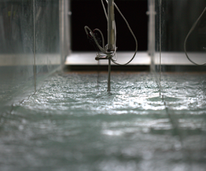
Experiments were carried out in a closed loop wind-wave facility that consists of a 5 m long test section made of glass and a wind tunnel atop of it; see figure 1. The test section is 0.4 m wide and 0.5 m high; the channel is filled with distilled water to depth 0.18 m. The airflow with velocity up to 13 m s $^{-1}$ is generated using a computer-controlled blower. The roof of the test section is made of removable Perspex plates with 3 cm wide slots in the centre, effectively sealed with fine brushes that enable introducing the sensors into the test section. The wind tunnel has inlet and outlet settling chambers, approximately 1 m $^3$ in volume each, so the air in those large chambers almost comes to rest. The airflow from the inlet chamber is guided through a honeycomb mesh into a converging nozzle connected to the test section that ensures parallel and uniform airflow at the entrance of the test section. The outlet settling chamber effectively eliminates back pressure fluctuations. A sloping beach made up of permeable mesh absorber is installed at the far end of the test section to reduce wave reflection. The water current in the test section is generated using a computer-controlled pump capable of generating mean velocity up to 0.20 m s $^{-1}$; the current velocity is determined by a rotary vane flow meter connected to a digital tachometer (SANYOU-FA 8). The valves attached at both ends of the test section enable changing the current direction. Water flows via holes in the bottom at both ends of the test section. The identical inlet and outlet water flow inlet/outlet devices with a small mixing chamber and a hexagonal honeycomb mesh are installed over those holes, with their openings to the test section facing the end walls. Thus for both flow directions, the in-flowing water passes through a honeycomb mesh to the mixing zone and then flows over the inlet section, resulting in a nearly uniform vertical water velocity profile in the upper half of the water layer (Kumar et al. Reference Kumar, Geva and Shemer2023). The instantaneous surface elevation $\eta (t)$ is measured using a set of five capacitance type wave gauges made of a pair of 0.5 mm in diameter tantalum wires; each wave gauge is supported by a horizontal bar placed along the test section, with a spacing of 10 cm between the adjacent gauges. The bar is attached to a vertical stage connected to a carriage that can be placed at any location along the fetch. For additional details on the facility and data acquisition procedure, see Liberzon & Shemer (Reference Liberzon and Shemer2011) and Zavadsky & Shemer (Reference Zavadsky and Shemer2018).

Figure 1. Schematic of the experimental facility with conventional wave gauges.
Measurements were carried out at carriage positions corresponding to the first probe placed at  $x = 100$, 150, 200, 250 and 300 cm from the inlet, thus covering 25 fetches along the test section. A Pitot tube placed 10 cm above the mean water surface is used for monitoring the air velocity during the experiment. The experiments were conducted at four blower settings; the representative wind velocities $U_a$ are presented in table 1. The corresponding friction velocities $u_{\ast }$, and wind velocities extrapolated to $z=10$ m above the mean water surface $U_{a,10}$ based on the vertical air velocity profiles measured in the presence of water current by Kumar et al. (Reference Kumar, Geva and Shemer2023), are also given in this table. The representative values of the friction velocities $u_{\ast }$ in table 1 for each wind velocity $U_a$ are also based on those measurements that were carried out at numerous fetches and current velocities $U_w$. The data were recorded for 900 s at 200 Hz channel $^{-1}$ at each wind velocity, carriage location, and the values of the water current $U_w = 0$, $\pm$0.06, $\pm$0.09 and ${\pm }0.12\ {\rm m}\ {\rm s}^{-1}$, the positive and negative signs denoting co-wind and counter-wind water flow direction, respectively.
Table 1. Representative maximum wind velocity  $U_a$, friction velocity $u_{\ast }$, and wind velocity estimated at the elevation above the water surface $z = 10$ m, $U_{a,10}$.

In a separate series of experiments, simultaneous measurements of surface elevation  $\eta (t)$ and its slope components were performed using an optical wave gauge. The instrument consists of a laser slope gauge (LSG) for measurement of instantaneous along-wind $\eta _x=\partial \eta / \partial x (t)$ and cross-wind $\eta _y=\partial \eta / \partial y (t)$ slope components, and a high-speed camera that is positioned outside the test section and is directed at the laser beam allowing determination of the instantaneous surface elevation $\eta (t)$. The LSG set-up consists of a position sensor detector (PSD), a Fresnel lens with a 9 inch focal length, a diffusive screen, and a 650 nm, 0.2 W laser diode. The laser beam is placed below the glass bottom of the test section and is directed vertically. The PSD records the laser spot location on the screen with spatial resolution 0.75 $\mathrm {\mu }$m, which is then translated into $\eta _x$ and $\eta _y$. The image of the laser beam that is visible in water and not in air is recorded by the camera; the coordinate of the beam tip is translated into the surface elevation. The camera and LSG thus measure the surface elevation and the slope components at the same location, and are synchronized using LabView software. For more details on the optical sensor and its working principle, see Zavadsky, Benetazzo & Shemer (Reference Zavadsky, Benetazzo and Shemer2017), Zavadsky & Shemer (Reference Zavadsky and Shemer2017a, Reference Zavadsky and Shemer2018) and Kumar et al. (Reference Kumar, Singh and Shemer2022). Continuous 900 s measurement of synchronous surface elevation and its two slope components were performed at the rate of 150 Hz channel $^{-1}$ at six locations along the fetch, $x = 120$, 180, 211, 245, 296 and 335 cm; wind and water-forcing conditions were identical to those in experiments with wave gauges.
3. Results
3.1. Effect of current on energy and steepness of young wind waves
Characteristic wave amplitudes are represented by the root mean square (rms) values of the instantaneous surface elevation and related to the wave energy  $E$ by $\eta _{rms}(x)=\overline {\eta ^2}(x)^{1/2}= E(x)^{1/2}$. The values of $\eta _{rms}$ are presented in figure 2 as a function of water current velocity $U_w$ at a single fetch $x = 245$ cm, and for all wind velocities. In the presence of turbulent mean water flow, the water surface in the test section ceases to be smooth. As expected, the values of $\eta _{rms}$ with no airflow in the test section applied, also plotted in figure 2, do not depend notably on the flow direction but grow with increase in water velocity. Figure 2 demonstrates that the relative contribution of irregularities at the surface induced by the mean water current to the resulting wind-wave field is insignificant. At all wind conditions, increase in water velocity $U_w$ in the wind direction has only a minor effect on $\eta _{rms}$. Contrary to that, when the mean current is directed against the wind, the characteristic wave amplitudes increase significantly with $|U_w|$.

Figure 2. Variation of characteristics wave amplitude  $\eta _{rms}$ as a function of water current velocity $U_w$ at $x = 245$ cm for different wind velocities $U_a$.
The variation with fetch of the characteristic wave amplitude  $\eta _{rms}(x)$, measured using both the conventional wave gauge (open symbols) and the optical wave gauge (solid symbols), is plotted in figure 3 for all wind velocities $U_a$. The dimensionless fetch $\hat {x}=x(g/u_{\ast }^2)$ and the dimensionless characteristic wave amplitude $\hat {\eta }_{rms}(x)=(g /(u_{\ast }^2))\eta _{rms}$ introduced by Kitaigorodskii (Reference Kitaigorodskii1961) are now adopted. The values of dimensionless fetch $\hat {x}$ in the present experiments vary from 30 to 243. The solid lines in figure 3 correspond to the fit $\eta _{rms}(\hat {x})=\hat {\eta }_0(u_{\ast }^2/g)\hat {x}^n$, where $\hat {\eta }_0=\hat {\eta }_{rms}(\hat {x}=1)$, with a single value of the exponent ( $n=0.5$) corresponding to the Mitsuyasu (Reference Mitsuyasu1970) law, which was adopted for all experimental conditions. The reference value of the dimensionless fetch $\hat {x}=1$ in the present experiments corresponds to a very short dimensional distance from the inlet of a few mm; the value of $\hat {\eta }_0$ can thus be seen as the effective dimensionless initial characteristic wave amplitude. For all wind velocities, water flow in the wind direction ( $U_w>0$) has no notable effect on $\hat {\eta }_0$; the reference value $\hat {\eta }_0=0.013$ estimated in the present experiments agrees reasonably well with the results of Wilson (Reference Wilson1965) and Mitsuyasu (Reference Mitsuyasu1970), as well as with the previous measurements in our facility (Zavadsky, Liberzon & Shemer Reference Zavadsky, Liberzon and Shemer2013; Shemer Reference Shemer2019). The values of $\hat {\eta }_0$ also remain unaffected by water current in the wind direction, $U_w>0$, for all wind velocities. For the counter-wind current case, however, the wave energy at each fetch increases notably with $|U_w|$, and the initial effective dimensionless wave amplitude increases from $\hat {\eta }_0=0.017$ for $U_w=-0.05$ m s $^{-1}$ to $\hat {\eta }_0=0.023$ for the strongest counter-current, $U_w=-0.12$ m s $^{-1}$.

Figure 3. Effect of water current  $U_w$ on variation with fetch $x$ of characteristic wave amplitude $\eta _{rms}$ for different values of the wind velocity $U_a$.
Time records of orthogonal slope components enable direct estimates of mean wave steepness defined as  $\overline {ak}=(\overline {\eta _x^2}+\overline {\eta _y^2})^{1/2}$ that is a measure of wave field nonlinearity. The variation with fetch $x$ of the wave steepness for two wind velocities, $U_a = 6.83$ m s $^{-1}$ and $U_a = 9.35$ m s $^{-1}$, presented in figure 4, shows that its values remain almost constant along the test section for both wind velocities $U_a$. Somewhat higher values of steepness were measured as the value of $U_a$ increases. In the absence of current, these results are consistent with the steepness behaviour reported by Zavadsky et al. (Reference Zavadsky, Benetazzo and Shemer2017), Zavadsky & Shemer (Reference Zavadsky and Shemer2017a). Mean water current in wind direction practically does not affect $\overline {ak}$, while the counter-wind current causes a slight increase in the wave steepness at all fetches (with a possible exception of the shortest one).

Figure 4. Effect of mean current on variation of mean steepness  $\overline {ak}$ along the fetch $x$ for two wind velocities $U_a$. Notation as in figure 2(a).
The effect of wind velocity  $U_a$ in the presence of water current is studied further in figure 5. The variation with current velocity $U_w$ plotted in this figure at a single fetch $x = 245$ cm for all wind velocities $U_a$ clearly demonstrates that the mean steepness $\overline {ak}$ increases with the wind velocity; the change in the steepness with $U_a$ does not depend significantly on $U_w$. For all wind and water velocities in the present experiments, the values of mean steepness exceed approximately 0.15, indicating that the young wind-wave field is notably affected by nonlinearity; the waves become very steep and attain high values of $\overline {ak} \approx 0.25$ for adverse water current. The shape of all curves in this figure is quite similar to that of the corresponding curves showing the variation of the characteristic wave amplitude with current in figure 2.

Figure 5. Effect of mean current  $U_w$ on variation of the mean steepness $\overline {ak}$ at $x = 245$ cm for all wind velocities $U_a$. Notation as in figure 2.
3.2. Variation of wave spectra with mean current
All spectra plotted in the sequel are based on 900 s long time records of  $\eta (t)$ for a given fetch $x$,
$x$,  $U_a$ and $U_w$ that are divided into 10 s long segments with 50 $\%$ overlap. The resulting spectrum represents the average of 180 power spectra computed for each segment with frequency resolution ${\rm \Delta} f = 0.1$ Hz. The variation with fetch of the surface elevation power spectra $E_{\eta } (f)$ at multiple locations is presented in figure 6 for wind velocity $U_a = 6.83$ m s $^{-1}$ and water current velocities $U_w = 0$ m s $^{-1}$ and $U_w =\pm 0.12$ m s $^{-1}$. The downshifting of peak frequency and increase in overall wave energy with fetch are clearly visible in both plots of this figure. The presence of current significantly modifies the spectral shapes. The counter-wind current (figure 6a) results in the spectrum dominated by longer waves with a lower peak frequency and much higher energy, compared to the wind-only power spectra in figure 6(b). The current in wind direction, while not affecting notably the total wave energy (cf. figure 3), results in spectra that are flatter and wider, with waves characterized by higher peak frequency and smaller amplitudes, including at the spectral peak; see figure 6(c).

Figure 6. Wave spectra  $E_{\eta }(f)$ at $U_a = 6.83$ m s $^{-1}$ and $U_w$ values (a) $-$0.12 m s $^{-1}$, (b) 0 m s $^{-1}$ and (c) 0.12 m s $^{-1}$.
The effect of the wind velocity  $U_a$ on the wave energy spectra $E_{\eta }(f)$ in the presence of current is examined further in figure 7 at a single fetch $x = 296$ cm for two extreme wind velocities. As expected, for each water current $U_w$, an increase in the wind velocity causes a rise in the peak spectral amplitudes accompanied by a decrease in peak frequencies. Figures 7(a,b) emphasize the notable effect of the water current on the spectral shapes, with the co-wind current resulting in a more uniform wave energy distribution among the frequency harmonic, while the opposite effect is observed for the counter-wind current.

Figure 7. Power spectra of surface elevation  $E_{\eta }(f)$ at $x = 296$ cm for (a) $U_a = 6.83$ m s $^{-1}$ and (b) $U_a=9.35$ m s $^{-1}$. Colour scheme as in figure 3.
Since the spectra plotted in figures 6 and 7 exhibit certain scatter, it is advantageous to use robust integral spectral moments to determine the dominant frequency  $f_{dom}$ as the principal statistical parameter, rather than the peak frequency $f_p$. The $j$th spectral moment of the omnidirectional power spectrum of the surface elevation $E_\eta (f)$ is defined as
 \begin{equation} m_j = \int_{f_{min}}^{f_{max}} f^j E_{\eta}(f) \,{\rm d} f, \quad j = 0, 1, 2,\ldots .\end{equation}
 The integration in (3.1) is carried out within the free wave domain around the peak frequency  $f_p$, defined here by $f_{min}=0.5f_p$ and $f_{max}=1.5f_p$. The imposed restriction limits the analysis to free waves only and eliminates the excessive contribution of second-order bound waves to higher-order spectral moments. The frequency $f_p$ for each spectrum is defined by applying the parabolic fit in the vicinity of the spectral peak. Note that the zeroth moment $m_0$ also defines the total energy of free waves; the adopted integration limits in (3.1) result in characteristic wave amplitudes that are somewhat below the $\eta _{rms}$ values; however, the difference is less than a few per cent. The dominant frequency $f_{dom}$, defined as
 \begin{equation} f_{dom} = m_1/m_0,\end{equation}
is less prone to experimental error than  $f_p$; however, the values of $f_{dom}$ and $f_p$ usually do not differ significantly. The variation of $f_{dom}$ with fetch is plotted in figure 8 for wind waves propagating over water with no mean current, as well as for the two extreme values of the water current velocity $U_w$. The plots correspond to each wind velocity $U_a$. The dominant frequency $f_{dom}$ decreases with fetch for all current conditions and wind velocities; for all operational conditions at any given fetch; $f_{dom}$ is higher for current in the wind direction, and lower for counter-wind water current, as compared to the corresponding $f_{dom}$ for $U_w = 0$. For all current conditions, the dominant frequency at all fetches decreases with an increase in current. The solid lines in figure 8 correspond to the power-law fit for the dependence of the dimensionless dominant frequency $\hat {f}_{dom}=f_{dom} (g/u_{\ast })$ on the dimensionless fetch $\hat {x}=x(g/u_{\ast }^2)$,
 \begin{equation} \hat{f}_{dom} = \hat{f}_{dom,0} (\hat{x})^{{-}1/3},\end{equation}
where the fitting coefficient is  $\hat {f}_{dom,0}=\hat {f}_{dom}(\hat {x}=1)$. Note that the fitting exponent in the power law for all cases in figure 8 is close to $n = -0.33$, as suggested for deep-water wind waves, in agreement with previous studies cited in relation to figure 3. The coefficient $\hat {f}_{dom,0}$ is close to unity in the absence of current, again in agreement with Mitsuyasu (Reference Mitsuyasu1970), Zavadsky et al. (Reference Zavadsky, Liberzon and Shemer2013) and Shemer (Reference Shemer2019). All curves for $U_w>0$ in figure 8 are above those corresponding to the $U_w=0$ cases. Accordingly, the reference values of $\hat {f}_{dom,0}$ are somewhat higher. The largest value of $\hat {f}_{dom,0} = 1.3$ is attained at low wind velocity; the effect of co-wind current decreases with an increase in $U_a$, approaching $\hat {f}_{dom,0} \approx 1$ at higher wind velocities. The values of $\hat {f}_{dom,0}$ in case of counter-wind current are consistently below unity and seem to be independent of $U_a$; they vary from $\hat {f}_{dom,0} \approx 0.57$ for $U_w = -0.12$ m s $^{-1}$ to $\hat {f}_{dom,0} \approx 0.78$ for $U_w = -0.05$ m s $^{-1}$.

Figure 8. Variation of the dominant frequency with fetch  $f_{dom}(x)$ for three values of the water current velocity $U_w$ and four values of the wind velocity $U_a$; colour scheme as in figure 3. Open symbols indicate wire gauge data; closed symbols indicate optical wave gauge data; solid lines indicate power-law fit.
3.3. Effect of current on statistical properties defined by higher spectral moments
Additional integral statistical parameters, such as dimensionless spectral width  $\nu$, skewness $\lambda _3$ and kurtosis $\lambda _4$, are now examined. The spectral wave energy concentration around $f_{dom}$ is estimated using the second-order central moment $\tilde {m}_2=\int (f-f_{dom})^2\,\hat {E}(f) \, {\rm d} f$; rendered dimensionless by $f_{dom}^2 m_0$, it defines the spectral width $\nu$ (Massel Reference Massel1996):
 \begin{equation} \nu = \sqrt{\frac{m_0 m_2}{m_1^2} - 1}.\end{equation}
 The values of  $\nu$ plotted in figure 9 for two wind velocities allow quantitative refinement of the qualitative assessment of the mean current effect on $\nu$ made by examining the spectral shapes in figures 6 and 7. For both wind velocities and at any given fetch $x$, the spectral width $\nu$ for the co-wind current conditions (figure 9c) is higher than that corresponding to the values of $\nu$ with no mean current (figure 9b) as observed in figures 6 and 7. In figures 9(b,c), the spectral width $\nu$ decreases slightly with fetch. In the absence of current, such a decrease in $\nu$ was reported by Zavadsky et al. (Reference Zavadsky, Liberzon and Shemer2013). For counter-wind current, no clear pattern can be seen in the dependence $\nu (x)$ in figure 9(a); for lower wind velocity $U_a$, the spectral width $\nu$ in this plot does not vary significantly with fetch and is comparable to that in figure 9(b) with $U_w=0$ m s $^{-1}$, while for $U_a = 9.35$ m s $^{-1}$, the values of the dimensionless spectral width show a tendency to grow with fetch.

Figure 9. Variation of the spectral width  $\nu$ with fetch for $U_w$ values (a) $-0.12$ m s $^{-1}$, (b) $0$ m s $^{-1}$ and (c) $0.12$ m s $^{-1}$, with $U_a = 6.83$ m s $^{-1}$ and 9.35 m s $^{-1}$.
Higher-order statistical moments such as skewness  $\lambda _3$ and kurtosis $\lambda _4$, as well as asymmetry $A$, provide additional insight into the effect of water current on the wind waves’ shape. These statistical parameters are presented in figures 10 and 12 as functions of water velocity $U_w$ for two values of $U_a$, i.e. $6.83$ m s $^{-1}$ and $9.35$ m s $^{-1}$, at three fetches, $x = 100$, 200 and 300 cm. The dimensionless $n$th-order moments are defined as
 \begin{equation} \lambda_n = \frac{\overline{\eta^n}}{\overline{\eta^2}^{n/2}}.\end{equation}
Figure 10. Variation with current velocity  $U_w$ of (a,c) skewness $\lambda _3$, and (b,d) kurtosis $\lambda _4$, at three fetches $x$ and wind velocities (a,b) $U_a = 6.83$ m s $^{-1}$ and (c,d) $U_a = 9.35$ m s $^{-1}$.
The third-order moment  $\lambda _3$ (skewness) characterizes wave asymmetry with respect to the horizontal axis. The positive skewness of gravity waves with notable steepness represents wave crests that are larger than troughs, mainly due to the contribution of second-order bound waves. The values of $\lambda _3$ plotted in figures 10(a,c) are indeed positive for all values of $U_w$. In the absence of mean current, the skewness of wind waves measured in the present facility for a wide range of wind velocities $U_a$ and several fetches by Zavadsky & Shemer (Reference Zavadsky and Shemer2017a) and Shemer (Reference Shemer2019) remains positive and tends to increase with $U_a$ and with fetch $x$; this result is confirmed in figures 10(a,c). For counter-wind current, $U_w<0$, the waves become steeper as the current becomes stronger; the more pronounced nonlinearity contributes to increase in $\lambda _3$. When wind and current are aligned, $U_w>0$, $\lambda _3$ decreases slightly with increase in $U_w$.
The fourth-order moment, kurtosis  $\lambda _4$, characterizes the wave height probability distribution; $\lambda _4=3$ corresponds to the normal (Gaussian) distribution. In the absence of current, the kurtosis does not vary notably with fetch and $U_a$, remaining close to $\lambda _4=2.5$, thus indicating that the wave height distribution is somewhat narrower than Gaussian. As seen in figures 10(b,d), this observation is still valid in the presence of current, although for $U_w>0$ the values of $\lambda _4$ tend to increase with $U_w$, tending to the Gaussian value $\lambda _4=3$. The effect of current on wave height distribution can also be examined by plotting the exceedance distribution function of wave height $h_w$ that for narrow-banded linear Gaussian waves has Rayleigh distribution
 \begin{equation} f(h_w) = \exp \left( -\frac{h_w^2}{8\overline{\eta^2}} \right) .\end{equation}
 The height  $h_w$ of each individual wave is defined as the difference between the consecutive crest and trough between two consecutive positive zero crossings; for more details, see Kumar et al. (Reference Kumar, Fershtman, Barnea and Shemer2021). The exceedance functions estimated at two extreme fetches $x = 100$ and 300 cm at $U_a = 6.83$ m s $^{-1}$ and water flowing in both directions are compared with the no-current case in figure 11 as a function of the normalized $h_w$. Note that for no-current and counter-wind current cases at fetch $x = 100$ cm, the characteristic wave height is still very small (see figure 3), the probability of higher waves with heights exceeding approximately $4\eta _{rms}$ is below that corresponding to the Rayleigh distribution. At higher fetch $x = 300$ cm, the probability of waves with $h_w>6\eta _{rms}$ falls below that of the Rayleigh curve. No extremely steep waves or rogue waves with heights exceeding $8\eta _{rms}$ were observed.

Figure 11. Exceedance distribution function  $F(h_w)$ of wave height $h_w$ at fetch $x$ values (a) $100$ cm and (b) $300$ cm, at $U_a = 6.83$ m s $^{-1}$, for $U_w = 0$ and ${\pm }0.12$ m s $^{-1}$.
The symmetry of the wave shape relative to the vertical axis is often defined using the differences in location between successive crests and troughs Babanin et al. (Reference Babanin, Chalikov, Young and Savelyev2010). However, for a three-dimensional random wind-wave field, Elgar & Guza (Reference Elgar and Guza1985) and Elgar (Reference Elgar1987) offered a more robust estimate of vertical wave asymmetry  $A$ based on the Hilbert transform $H(\eta )$ of the measured surface elevation $\eta (t)$:
 \begin{equation} A ={-}\frac{\overline{{\rm Im}(H(\eta))^3}}{\overline{\eta^2}^{3/2}}.\end{equation}
 The wave asymmetry  $A$ calculated according to (3.7) plotted in figures 12(a,b) is positive for all fetches and all current velocities, indicating that for young wind waves, the windward part of the wave is on average longer than the leeward part. In the absence of current, the asymmetry $A$ decreases somewhat with fetch, in agreement with observations by Shemer (Reference Shemer2019); both co- and counter-wind currents tend to decrease the asymmetry with an increase in absolute current velocity.

Figure 12. Variation with current velocity  $U_w$ of asymmetry $A$ at three fetches $x$ and wind velocity $U_a$ values (a) $6.83$ m s $^{-1}$ and (b) $9.35$ m s $^{-1}$.
3.4. Dispersion relation in presence of current
The Doppler-shifted linear dispersion relation for gravity-capillary waves propagating over uniform current with velocity  $U_w$ is
 \begin{equation} (\omega - k U_w)^2=\left( gk+\frac{\sigma}{\rho}\,k^3 \right) \tanh{kh},\end{equation}
where  $\omega = 2{\rm \pi} f$ is the angular frequency, $\rho$ is the water density, $\sigma$ is the water surface tension, and $h$ is the water depth. Single-point synchronous measurement of surface elevation and surface slope components $\eta _x$ and $\eta _y$ allows direct determination of the relation between the wave frequency and the absolute value of its wave vector $k(f)=(k_x^2(f)+k_y^2(f))^{1/2}$. In the absence of mean current, those spectra have been presented in Zavadsky & Shemer (Reference Zavadsky and Shemer2017a); the present study examined the power spectra $E_{\eta _x}=k_x^2\,E_{\eta }(f)$ of $\eta _x(t)$, and $E_{\eta _y}=k_y^2\,E_{\eta }(f)$ of $\eta _y (t)$, and found that they are not affected qualitatively by the mean current and therefore not given here. The wavenumber $k(f)$ as a function of frequency $f$ is determined from the power spectra of the synchronous single-point measurements of $\eta (t)$, $\eta _x(t)$ and $\eta _y(t)$ as in Longuet-Higgins, Cartwright & Smith (Reference Longuet-Higgins, Cartwright and Smith1961):
 \begin{equation} k(f) = \sqrt{\frac{E_{\eta_x}(f)+E_{\eta_y}(f)}{E_{\eta}(f)}}.\end{equation}
 In the present experiments, wavenumbers  $k(f)$ estimated at each fetch $x$ at dominant frequency $f_{dom}(x)$ are plotted in figure 13; the error bars represent the standard deviation of $k(f)$ estimated at frequencies around $f_{dom}(x)$ that satisfy the condition on the magnitude squared coherence, $M_{\eta \eta _x}=|E_{\eta }^{\ast }E_{\eta _x}|^2/(E_\eta E_{\eta _x})>0.8$. At any given frequency $f$, due to wind-induced shear current, the experimentally determined wavenumbers $k$ for wind waves in the absence of current are consistently below those corresponding to the gravity-capillary dispersion relation, $k_{gc}$. This effective Doppler shift is accounted for in the empirical dispersion relation by Zavadsky & Shemer (Reference Zavadsky and Shemer2017a) in the form
 \begin{equation} \frac{k_{gc}(f)}{k} = 1+ak+bk^2,\end{equation}
where  $a=0.006$ m and $b=-2.2\times 10^{-5}\ {\rm m}^{2}$ are the empirical fitting coefficients and agree well with the present experimental results.

Figure 13. Dominant wavenumber  $k_{dom}$ as a function of frequency $f_{dom}$.
The ratio  $k_{gc}/k$ suggested in the dispersion relation by Zavadsky & Shemer (Reference Zavadsky and Shemer2017a) is substituted into (3.9) to account for additional Doppler shift induced by uniform current $U_w$; the result is plotted in figure 13 by solid lines. For co-wind current, the dominant frequencies $f_{dom}$ are shifted to higher values, and for counter-wind current they are shifted to lower values, as compared to the no-current case. The empirical dispersion relation by Zavadsky & Shemer (Reference Zavadsky and Shemer2017a) seems to retain its validity also in the presence of uniform current.
3.5. Temporal coherence of wind waves propagating over mean current
To illustrate the essentially random nature of wind waves with and without mean current, it is instructive to look at the temporal variation of the ‘amplitude’ of instantaneous ‘frequencies’ using wavelet analysis (Kumar & Shemer Reference Kumar and Shemer2024). The 20 s long Morlet spectrograms starting at  $t = 20$ s are plotted in figure 14 for a single fetch $x$, a single wind velocity $U_a$, and two extreme values of water current; the spectrogram in the absence of mean water current is also presented for comparison. The vertical section of the wavelet ‘spectrum’, or ‘map’, at any time $t$ provides an instantaneous ‘amplitude’ as a function of frequency $f$. The horizontal solid lines in all plots of figure 14 correspond to the dominant frequency $f_{dom}(x = 245\ {\rm cm})$ plotted in figure 8. The characteristic frequencies at which the highest amplitudes in each wavelet spectrogram are attained indeed agree well with their corresponding $f_{dom}$.

Figure 14. Wavelet spectrograms of surface elevation  $S_\eta (f,t)$ as functions of frequency and time a $x = 250$ cm and $U_a = 6.83$ m s $^{-1}$, for three values of $U_w$.
At all current velocities, the spectrograms exhibit significant variability with time, thus confirming the essentially random character of wind waves, as demonstrated in figure 14. To quantify the effect of mean water current on the temporal wave coherence, the auto-correlation analysis of the temporal records of  $\eta (t)$ is studied here. The dependence of the auto-correlation coefficient $R(\tau )$ on the time shift $\tau$ for a function with zero mean $F(t)$ is defined as (Bendat & Piersol Reference Bendat and Piersol1971)
 \begin{equation} R(\tau) = \frac{\overline{F(t)\,F(t+\tau)}}{\overline{F^2}}.\end{equation}
 Statistically reliable estimates of  $R$ are obtained by computing the values of $R(t)$ over each one of the 10 s long segment cuts of the whole record, and averaging the outcome over all segments. The resulting averaged auto-correlation coefficient is plotted in figure 15 at two extreme fetches, $x = 100$ and 300 cm, for two extreme current velocities. The lag $\tau$ is normalized by the local dominant frequency $f_{dom}$ (see figure 8). In each plot, the values of $R$ oscillate at the local dominant frequency and decay within a few dominant wave periods. The decay of the local maximum of the auto-coherence coefficient at each fetch $x$ is approximated by an exponent as ${\sim }{\rm e}^{-\alpha _d(\tau /T_d)}$, where $\alpha _d$ is the dimensionless decay rate. In the absence of mean current, the decay rate $\alpha _d$ in figure 15(b) decreases with fetch and thus with the wavelength, in agreement with Shemer & Singh (Reference Shemer and Singh2021) and Kumar et al. (Reference Kumar, Singh and Shemer2022). Waves propagating over water flowing against the wind retain their coherence longer compared to waves in the absence of current, while waves propagating over co-wind current lose their coherence within less than one dominant wave period; see figure 15(c).

Figure 15. Temporal coherence function  $R(\tau )$ at $U_a = 6.83$ m s $^{-1}$ and $U_w$ values (a) $-0.12$ m s $^{-1}$, (b) 0 m s $^{-1}$ and (c) 0.12 m s $^{-1}$.
The dimensionless decay rates  $\alpha _d$ for all operational conditions employed in the present experiments are summarized in figure 16 for all forcing conditions; they are presented as functions of dominant wavelength $\lambda _{d}$. For the reference wind-only cases, decay rate $\alpha _d$ decreases with increase in both wind velocity and wavelength, in agreement with Shemer & Singh (Reference Shemer and Singh2021). The dimensionless decay rates for waves in the absence of mean current and for counter-wind current show similar dependence on $\lambda _{d}$. Contrary to that, for the along-wind current, the values of $\alpha _d$ are significantly higher and widely spread.

Figure 16. Dimensionless decay rate  $\alpha _d$ as a function of dominant wavelength $\lambda _d$ for all wind velocities.
3.6. Two-dimensional characterization of the wind-wave field in the presence of current
The two simultaneously measured slope components allow two-dimensional characterization of the instantaneous surface by projecting the vector normal to the surface on the horizontal plane. Instantaneous surface slope is defined as  $\theta = \arctan (\eta _y/\eta _x)$. The probability distribution function (p.d.f.) of instantaneous surface slope at a single fetch and for all wind forcing conditions is presented in figure 17 for extreme values of current velocities and compared with $U_w = 0$ m s $^{-1}$.

Figure 17. The p.d.f.s of instantaneous surface slope  $\theta$ at fetch $x = 335$ cm for $U_w$ values (a) $-0.12$ m s $^{-1}$, (b) $0$ m s $^{-1}$ and (c) $0.12$ m s $^{-1}$.
All p.d.f.s in figure 17 are characterized by two distinctive peaks at  $\theta = 0$ and ${\rm \pi}$, indicating the prevailing direction of waves along the wind. For all wind and current forcing conditions, the probability of a forward-leaning slope ( $\theta = 0$) is smaller than that of the windward slope at $\theta = {\rm \pi}$, showing front–back asymmetry. This asymmetry decreases with an increase in wind velocity, and nearly vanishes when stronger wind forcing is applied. For a given wind velocity, the angular asymmetry behaves similarly for co-wind current and no-current conditions, while in counter-wind current, the angular distribution approaches the symmetrical one. This is in agreement with the asymmetry plotted in figure 12. For a random wind-wave field with directional spreading, the probability of a wave vector normal to the surface that is perpendicular to the mean wind direction, $\theta =\pm {\rm \pi}/2$ is non-negligible for all wind and water current conditions. Though there is a well-defined wave asymmetry along the wind direction as documented in figures 17 and 12, there is a left–right symmetry near the vicinity of $\theta =\pm n {\rm \pi}/2$, thus effectively showing cross-wind symmetry of the p.d.f.
4. Discussion
The experimental findings on the effect of velocity and direction of mean water flow on the statistical parameters of young wind waves presented in the previous section may seem somewhat contradictory. On one hand, figure 2 suggests that when water flows in the wind direction, the current velocity  $U_w$ seems to have only a minor effect on the characteristic wave amplitudes at a given fetch. At those water flow conditions, figure 3 demonstrates that the variation with fetch of the total wave energies $E(x) = \eta _{rms}^2$ is also not affected significantly by $U_w$, and remains approximately linear with $x$ for all wind velocities $U_a$. Similarly, the fetch dependence of the dominant frequency $f_{dom}(x)$ is only weakly affected by the presence of the co-wind mean water current; the upshifting of $f_{dom}$ due to the Doppler shift for $U_w>0$ becomes noticeable only at lower wind velocities (see figure 8). Contrary to that, the counter-wind water current, $U_w<0$ affects notably both the wave energy and the dominant wave frequency. At all wind velocities, the characteristic wave amplitudes $\eta _{rms}$ grow when the water flow rate in the counter-wind direction increases in figure 2, while the Doppler downshift of the dominant frequency $f_{dom}$ becomes more pronounced, as seen in figure 8. It should be stressed that the spatial changes in both $\eta _{rms}$ and $f_{dom}$ in the presence of mean current in both directions still comply with the Mitsuyasu (Reference Mitsuyasu1970) law that states that both the total wind-wave energy and the dominant frequency evolve as a power of the dimensionless fetch. The effect of current manifests itself only in the values of the empirical scaling coefficients that define the initial conditions as shown in figures 3 and 8.
It is therefore somewhat surprising that while the total wave energy and the dominant frequency for each wind velocity remain only weakly sensitive to the co-wind water current, the spectral shapes in this case vary significantly with  $U_w$, as shown in figures 6 and 7. For each wind velocity, the co-wind current causes apparent widening of the spectra, while water current in the counter-wind direction has an opposite effect on the spectral energy distribution, so that the spectra for $U_w<0$ look narrower than those in the absence of the mean current. This is also evident in the wavelet spectrograms presented in figure 14, which show broadening of the range of instantaneous ‘frequencies’ with substantial amplitudes with an increase in the mean water velocity $U_w$ from negative to positive. Variation of the dimensionless spectral width $\nu$ with fetch plotted in figure 9 supports this conjecture quantitatively.
The approach to analysis of the spatial and temporal evolution of a random wind-wave field suggested by Geva & Shemer (Reference Geva and Shemer2022) (referred to here as the GS model) is now applied to provide a framework to understanding the modifications of the essential wind-wave statistical parameters due to the presence of mean water current that are identified in this study. In the quasi-linear GS model, the random wave field is seen as a stochastic ensemble of multiple harmonics, each harmonic growing due to shear flow instability with the growth rate obtained by solving the coupled Orr–Sommerfeld (OS) equations in air and in water. While the initial growth of each harmonic is exponential due to linearity of the OS equations, at a later stage it is capped by the essentially nonlinear effects of breaking and sheltering. The GS model utilizes the experimentally determined fact that for a given wind velocity  $U_a$, the friction velocity $u_{\ast }$ that characterizes the momentum exchange between wind and waves does not vary significantly with fetch (Zavadsky & Shemer Reference Zavadsky and Shemer2012). The GS model was successfully verified by carrying out comparison of the model prediction with detailed measurements of the temporal and spatial variation of the wave field from initially quiescent surface to rough quasi-steady state under impulsively applied wind (Zavadsky & Shemer Reference Zavadsky and Shemer2017b).
Kumar & Shemer (Reference Kumar and Shemer2024) examined the GS approach further to study experimentally the spatial variation of energy of individual harmonics in the gravity-capillary range of frequencies that characterizes a young fetch-limited wind-wave field excited by steady forcing. They demonstrated that the frequency spectrum at very short fetches is broad, so that the wave energy  $E(f_i)$ is distributed nearly uniformly among multiple small-amplitude harmonics. Each such harmonic indeed initially grows exponentially with fetch, $E(f_i, x) = E(f_i, x_0) \exp [\alpha _i(x-x_0)]$, where $E(f_i, x_0)$ is the energy of the $i$th harmonics at the initial short fetch $x_0$; its spatial growth rate $\alpha _i$ decreases with decreasing frequency, in agreement with computations based on the OS viscous shear flow instability model by Zeisel, Stiassnie & Agnon (Reference Zeisel, Stiassnie and Agnon2008).
Kumar & Shemer (Reference Kumar and Shemer2024) demonstrated that the quasi-linear GS approach leads to the distinction between the factors that limit the growth of harmonics at different frequencies. The exponential growth of shorter harmonics in the spectrum ceases at a fetch where the limiting wave steepness  $\overline {ak}_{lim}$, mostly determined by the amplitude of waves around the local dominant frequency, is attained. Shorter harmonics are sheltered by the relatively high local dominant one, and cease to grow, while long waves with smaller growth rates still have low amplitudes and small steepness at those fetches. Those long waves are not affected by sheltering due to their length scales, and therefore continue to grow. At a more distant fetch, those longer harmonics may attain amplitude that exceeds that of all other spectral harmonics and thus become the dominant ones in the wave field. The eventual height of the longer spectral harmonics is defined by their initial amplitude, the growth rate and the maximum possible for a given fetch $x$ duration of growth $\tau (x,f)=x/c_g(f)$. The GS model therefore elucidates the mechanism by which the dominant frequency of wind waves downshifts with fetch. The model allows us to resolve the apparent contradiction between the exponential growth rate of individual harmonics predicted by the linear shear flow instability model, and the close to linear growth with fetch of the total wave energy of the ensemble of all spectral harmonics as observed in experiments.
The viscous unidirectional shear flow instability approach is now modified to account for steady mean current. In the GS model, the temporal growth rate of each harmonic with the wavenumber  $k$ is obtained under the assumption of spatial homogeneity as $\gamma (k)={\rm Im}\{ \omega (k)\}$, the complex radian frequency $\omega (k)$ being the eigenvalue of the OS problem; the real part ${\rm Re}\{ \omega (k) \}$ determines the dispersion relation. Experiments of Kumar et al. (Reference Kumar, Geva and Shemer2023) demonstrated that for a given wind velocity in the test section, the values of $u_{\ast }$ are not affected significantly by water velocity $U_w$ and remain approximately constant along the fetch. Since $|U_w | \ll U_a$, and the friction velocity $u_{\ast }$ that determines the slope of the mean air velocity profile does not change notably with water current, the Galilean transformation to a frame of reference moving with the constant current velocity $U_w$ does not affect the eigenvalues $\omega (k)$ of the OS problem. Figure 13 indeed demonstrates that the mean water current Doppler shifts only the wave frequencies that correspond to Re $\{ \omega (k) \}$ by $kU_w$; see (3.8). Smeltzer et al. (Reference Smeltzer, Æsøy, Ådnøy and Ellingsen2019) recently developed a sophisticated technique to estimate the Doppler-shifted dispersion relation based on any complicated water current profile. However, the empirical correction to the wavenumber $k$ in the presence of wind-induced shear current relative to the wavenumber that corresponds to the gravity-capillary dispersion relation $k_{gc}$ suggested by Zavadsky et al. (Reference Zavadsky, Benetazzo and Shemer2017) remains applicable also in the presence of mean water current.
Similarly, the temporal growth rate  $\gamma (k)$ for a given wavenumber that represents the imaginary part of the complex eigenfrequency, ${\rm Im}(\omega )$, is practically unaffected by the mean water current, thus enabling extension of the random unidirectional shear flow instability approach to study the evolution of wind waves in the presence of mean water current. However, wind waves under steady forcing grow in space rather than in time; the spatial growth rate $\alpha$ of each frequency harmonic is related to its temporal growth rate $\gamma$ by the wave energy propagation (group) velocity as $\alpha =\gamma /c_g$, as shown by Gaster (Reference Gaster1962) and confirmed by Zeisel et al. (Reference Zeisel, Stiassnie and Agnon2008) in their numerical studies of spatial and temporal instability governed by coupled OS equations. The measured spatial growth rates $\alpha (f)$ for the fetch-limited waves are usually translated into the temporal growth rates $\gamma (f(k))$ to enable comparison with additional experimental data (see Mitsuyasu & Honda Reference Mitsuyasu and Honda1982; Peirson & Garcia Reference Peirson and Garcia2008; Zhang et al. Reference Zhang, Hector, Rabaud and Moisy2023; Kumar & Shemer Reference Kumar and Shemer2024; and references therein).
Wave parameters in laboratory or field experiments are typically measured by fixed sensors as a function of frequency. Since the temporal growth rates  $\gamma (k)$ of harmonics defined by their lengths (rather than frequencies) remain unaffected by $U_w$, it is advantageous to base the study of mean water flow effect on the spatial evolution of wind waves on wavenumbers $k$ rather than on frequencies $f$. To this end, growth rates $\gamma (k)$ calculated applying the coupled OS equations (Kawai Reference Kawai1976; Valenzuela Reference Valenzuela1976; Tsai, Grass & Simons Reference Tsai, Grass and Simons2005; Zeisel et al. Reference Zeisel, Stiassnie and Agnon2008; Geva & Shemer Reference Geva and Shemer2022) can be used. Those computations are sensitive to the adopted shape of the velocity profiles in air and in water that correspond to the initially undisturbed water surface, as presented in the experiments of Caulliez, Ricci & Dupont (Reference Caulliez, Ricci and Dupont1998), where it was shown that the wind-induced drift current significantly affects the spatial growth rate of initial wavelets. However, waves excited by steady wind modify the air velocity profile (Kumar et al. Reference Kumar, Geva and Shemer2023); moreover, turbulent water flow introduces significant disturbances at the surface even in absence of wind; see figure 2. Since the present study is aimed at gaining a better understanding of the mean water flow effect on wind waves, the empirical relation for $\gamma (k)$ suggested by Plant (Reference Plant1982) for deep-water gravity waves is chosen here for this purpose.
For a given wind velocity  $U_a$ and mean water velocity $U_w$, the frequency $f$ that corresponds to each wavelength $\lambda =2{\rm \pi} /k$ is calculated using the dispersion relation (3.8), with the empirical fit (3.10) to account for wind-induced shear current suggested for short young wind waves by Zavadsky et al. (Reference Zavadsky, Benetazzo and Shemer2017). For a given wavelength, the wind-wave frequency $f(k)$ measured by a fixed sensor may vary dramatically with $U_w$, in co-current flow being higher than $f(k_i)$ in absence of mean water flow, and lower in counter-wind current; see figure 13 and § 3.4. The Doppler shift induced by the mean current also strongly affects the propagation velocity of the energy of each harmonic, $c_g(f)=2{\rm \pi} \, {\rm d} f/ {\rm d} k$, that relates the temporal $\gamma (k)$ and spatial $\alpha (f(k_i)) = \gamma (f(k_i))/c_g(f_i)$ growth rates (Gaster Reference Gaster1962). The group velocities for the two values of co- and counter-wind water current $U_w$ used in this study are compared in figure 18(a) with $c_{g,0}(f)$ that represent the group velocity of wind waves in the absence of mean water flow. For a given wavenumber harmonic $k$, the group velocity is modified by the mean current as $c_g = c_{g,0} + U_w$. The slowly propagating short waves in counter-wind water flow may get blocked by the opposing water current. The group velocities $c_g$ plotted in figure 18(a) for $U_w<0$ are thus truncated at $f = 6$ and 3 Hz for $U_w = -0.09$ m s $^{-1}$ and $-0.12$ m s $^{-1}$, respectively, frequencies at which the velocity of propagation with wind of wave energy in the presence of current, $c_{g}$, equals the counter-wind water velocity (Mei Reference Mei1989).

Figure 18. (a) Variation with frequency of group velocity  $c_g(f_i)$ as a function of frequency $f$. (b) Growth rate coefficient $\alpha (\lambda _i)$ as a function of wavelength $\lambda$ in the presence of current; the vertical black solid line at $\lambda =4$ cm corresponds to the waves with 8 Hz frequency in the absence of current.
For each frequency harmonic  $f(k_i)$, the temporal growth rate is calculated using the Plant (Reference Plant1982) empirical relation
 \begin{equation} \gamma(f(k_i)) = \beta\,\frac{\rho_a}{\rho_w} \left(\frac{u_{{\ast}}}{c}\right)^2 \omega.\end{equation}
 The spatial growth rates  $\alpha (\lambda _i)$ estimated using (4.1) and $c_g(f_i)$ plotted in figure 18(a) are presented in figure 18(b) as function of wavelengths $\lambda$. Since the empirical fit (3.10) based on data accumulated in the absence of current is valid up to wind-wave frequencies $f<8$ Hz (i.e. waves longer than $\lambda \approx 4$ cm), waves shorter than this limit are not considered in this figure.
The temporal growth rate  $\gamma$ decreases, and the group velocity $c_g$ increases with increase in wavelength, resulting in a sharp decrease of the spatial growth rate $\alpha$ with $\lambda$. Hence at each frequency, the spatial growth rate in the co-wind water flow is significantly smaller than in the absence of current. The wave field in the co-wind current is thus characterized by a wide spectrum of frequencies, including relatively long waves that – due to their advection by mean current – have higher frequency but low growth rates. This observation clarifies why the spectra in figure 6(c) are broad and contain numerous harmonics with amplitudes comparable to the no-current case. Although the spectra in along-wind current are characterized by relatively small amplitudes, the total energy $\eta _{rms}^2$ that represents the time-averaged contribution of multiple random frequency harmonics is not very different from the no-current case; see figure 3.
The higher values of  $\alpha (\lambda _i)$ for harmonics in counter-wind water flow result in the rapid growth of shorter harmonics up to the limiting maximum steepness; they then decay due to various nonlinear mechanisms, as discussed in detail in Kumar & Shemer (Reference Kumar and Shemer2024), while long waves continue their relatively slow growth but attain higher amplitudes. The narrow frequency spectrum at all fetches in figure 6(a) is also associated with the blockage of the shorter waves with $c_g(\lambda _i)+U_w \leq 0$ by counter-wind current that prevents their propagation in the wind direction; note that in our experiments with counter-wind current, $|U_w|/c_{g,0}(\lambda _i)$ is between 0.22 and 0.37. This limit imposed on wave energy propagation direction results in the dominant frequency $f_{dom}(x)$ that for $U_w = -0.12 \pm 0.01$ m s $^{-1}$ remains consistently below blocking frequency 3.5 Hz at all fetches and at all wind velocities; see figure 8.
Variation with fetch of the length of the dominant wave  $\lambda _d$ for two wind velocities is presented as a function of the water current velocity $U_w$ in figure 19. Although the Doppler shift in co-wind water flow results in waves with higher frequency, the values of $\lambda _d$ remain comparable with those in the wind-only case. The counter-wind water flow fosters propagation and growth of longer waves along the wind, while higher-frequency waves can be generated only locally, and decay. As depicted in figure 3, the characteristic wave energy $\eta _{rms}^2$ is higher and is comparable with the no-current case for counter- and co-wind water flow, respectively. This combined effect of variation of $\eta _{rms}^2$ and $k$ results in the representative wave steepness $\eta _{rms}k$ that is almost unaffected by current and remains nearly constant along the fetch; see figure 4. The conjecture adopted in the GS model that the wave steepness limits the growth of each wave harmonic is thus also applicable in the presence of current.

Figure 19. Variation of wavelength  $\lambda _d$ as a function of water current velocity $U_w$ for $U_a$ values (a) 6.83 m s $^{-1}$ and (b) 9.35 m s $^{-1}$.
The water current also notably affects the temporal coherence of wind waves. In the absence of current, wind-generated waves retain coherence up to 3–4 dominant wave periods  $T_d$, in agreement with Shemer & Singh (Reference Shemer and Singh2021), Kumar et al. (Reference Kumar, Singh and Shemer2022) and references therein. In counter-wind current, the wave field dominated by longer waves with narrower spectrum retains higher temporal coherence for multiple dominant wave periods. The rate of coherence decay $\alpha _d$ decreases with length of the dominant wave $\lambda _d$ for no-current and counter-wind water current; see figure 16. The presence of multiple coexisting harmonics with random phases in the co-wind current results in rapid loss of coherence that occurs after a single dominant wave period (see figure 15c), as well as in notably higher values of coherence decay rate coefficient $\alpha _d(\lambda _d)$.
5. Conclusions
To assess the effect of mean water current on generation of surface waves by steady wind, detailed measurements of the statistical wave parameters were carried out in a laboratory wave tank. Experiments were performed for a range of wind velocities  $U_a$; for each $U_a$, experiments were carried out for several mean water flow velocities $U_w$, in both co-wind and counter-wind directions. For each $U_a$ and $U_w$, measurements of the instantaneous surface elevation were carried at multiple densely spaced locations along the test section. In addition, synchronous measurements of the instantaneous surface elevation and of the two orthogonal slope components performed at several fetches for all operating conditions allowed the extraction of data on the water flow effect on the directional properties of wind waves.
In the absence of current, the characteristic wave energy  $\eta _{rms}^2$ and the dominant wave frequency $f_{dom}$ that characterize the fetch-limited wind-wave field follow the Mitsuyasu (Reference Mitsuyasu1970) power laws. It is demonstrated that these empirical relations remain valid also in the presence of current; the mean water flow affects only the conditions at the inlet, expressed through the initial dimensionless roughness $\hat {\eta }_0$ and the dimensionless frequency $\hat {f}_0$, which are affected by the surface roughness generated in the test section by the turbulent water flow.
Morlet wavelet spectrograms of the measured surface elevation were computed to assess the effect of mean water flow on the random character of the wind-wave field. The vertical slice of the spectrogram ‘map’ at any time  $t$ thus gives an instantaneous wavelet ‘amplitude map’ as a function of characteristic frequency $f$. For all experimental conditions, the spectrograms clearly demonstrate that the wave field is stochastic, and the instantaneous ‘frequencies’ corresponding to the maximum instantaneous wave energy vary significantly with time. For mean water current aligned with wind, the spectrogram ‘map’ has comparable ‘amplitudes’ for a range of frequencies, with no pronounced characteristic frequency. In counter-wind current, the wavelet spectrogram exhibits significantly higher amplitudes, with a significantly narrower range of energy-containing instantaneous wind-wave ‘frequencies’.
The quantitative statistically reliable characterization of the wave energy distribution among frequencies observed in the wavelet spectrograms was carried out by analysing the variation of the surface elevation power spectra with fetch for different operational conditions. Along the whole test section, waves propagating over co-wind current indeed have smaller spectral amplitudes distributed over a broad range of frequencies, while the counter-wind current wave field is dominated by longer waves with higher amplitudes in notably narrower spectra. The variation with the fetch of the spectral width  $\nu$ defined by (3.4) for different current settings is presented.
The effect of current on the shape of wind waves is investigated using integral statistical moments, such as the third-order moment  $\lambda _3$ (skewness) and the fourth-order moment $\lambda _4$ (kurtosis), as well as asymmetry $A$. The variation with water velocity $U_w$ of those parameters is presented for several fetches and wind velocities $U_a$. The temporal coherence is also notably affected by mean water current at each fetch and wind velocity; the rate of decay of the temporal coherence $\alpha _d$ increases when the current velocity changes from counter-wind to co-wind direction.
The synchronous single-point measurement of surface elevation and the orthogonal slope components enable direct estimates of wavenumber  $k$ as a function of frequency $f$. In the absence of mean current, the experimentally determined wavenumber $k$ follows the empirical expression proposed by Zavadsky et al. (Reference Zavadsky, Benetazzo and Shemer2017) that allows us to estimate the effect of the wind-induced shear water current on the variation of the wind waves’ length relative to that predicted by the linear gravity-capillary dispersion relation. This empirical estimate of the wind-induced current effect appears to be applicable in the presence of mean water flow as well. For each wavenumber $k$, the effect of water current on frequency $f$ is expressed solely by the mean flow-induced Doppler shift $kU_w$.
The experimental findings accumulated in this study on the variation of diverse wave statistical parameters in the presence of current are discussed in the framework of the viscous shear flow instability model of Geva & Shemer (Reference Geva and Shemer2022). As assumed in their approach, at all operational conditions, the wave energy at the inlet is distributed nearly uniformly among multiple wavenumber harmonics. The energy of each wave harmonic then increases along the test section due to viscous shear flow instability. It is shown in this study that the temporal growth rates  $\gamma (k)$ that govern the initial exponential wave energy growth of each harmonic are practically not affected by mean current. The group velocity of each harmonic $c_g(k(f))$ at which the energy of harmonic propagates along the test section, however, varies notably with mean current $U_w$, being larger for co-wind current and smaller for counter-wind water flow, as compared to $c_g$ in the absence of mean current. The spatial growth rate $\alpha (f)$ for each wavenumber $k$ and the corresponding Doppler shifted frequency $f(k)$, i.e. $\alpha (f)= \gamma (f(k))/c_g(f(k))$, is thus affected significantly by the mean current.
In a fetch-limited wind-wave field under steady wind forcing, the initial spatial exponential growth of each harmonic with its growth rate  $\alpha (f)$ is limited by the maximum possible steepness. The present results show that the limiting steepness remains unaffected by the mean flow. Alternatively, the evolution of the energy of each harmonic along the tank can be seen as its growth in time while it propagates along the test section from the inlet to fetch $x$ with the exponential temporal growth rate $\gamma (f(k))$. In this interpretation, the upper limit on the possible duration growth of each harmonic is given by $\tau (f(k))=x/c_g(f(k))$. Due to variation of the group velocity for a given $k$ with the mean flow $U_w$, $\tau (k)$ of each harmonic in co-wind current decreases, whereas it increases significantly in counter-wind water flow. Therefore, in a test section of a fixed length, presence of current notably modifies the effective length available for the growth of each harmonic. The faster evolving with fetch $x$ waves in counter-wind current thus make the test section effectively longer, while co-wind current reduces the available length. The variation of effective length of the test section in the presence of current thus clarifies the observed variation of the spatial growth rates $\alpha (f)$ in the presence of mean water current, and the resulting effect on wind-wave statistical parameters.
Funding
This work was supported by the Israel Science Foundation (grant no. 735/23).
Declaration of interests
The authors report no conflict of interest.


 Open access