


1. Introduction
Surface roughness elements of boundary layer size and smaller are ubiquitous and have a crucial influence on flow instability and laminar–turbulent transition. The velocity streaks generated by the so-called lift-up effect (Landahl Reference Landahl1980) had long been believed to trigger earlier transition, until the work of Cossu & Brandt (Reference Cossu and Brandt2004) and Fransson et al. (Reference Fransson, Talamelli, Brandt and Cossu2006) demonstrated that the streaky flow produced by roughness arrays is also capable of delaying laminar–turbulent transition. This motivated additional investigations of transition delay methods with roughness elements in both two-dimensional (2-D) (Fransson et al. Reference Fransson, Talamelli, Brandt and Cossu2006) and three-dimensional (3-D) (Saric, Carpenter & Reed Reference Saric, Carpenter and Reed2011) boundary layers, due to the fact that a successful transition delay technology has a great benefit in the reduction of operational costs for moving vehicles and engineering parts or processes.
The laminar–turbulent transition process in a Blasius boundary layer can take several paths depending on the level of external disturbances (Morkovin Reference Morkovin1994), like free stream turbulence, surface roughness or controlled excitation. At low levels of excitation, linear stability theory (LST) reveals the contribution of Tollmien–Schlichting (TS) waves, which are 2-D, viscous and grow exponentially. As the amplitude of the TS-wave grows to 1 % of the free stream velocity, secondary instability sets in and it quickly breaks down into turbulence (Kachanov Reference Kachanov1994). At higher external disturbance levels, very weak streamwise vortices are able to push high-speed fluid towards the wall and the low-speed fluid to the opposite direction, i.e. the lift-up mechanism (Landahl Reference Landahl1980), thus creating elongated streamwise streaks. In such circumstances, a transient algebraic increase of the perturbation, which is due to the non-normality of the controlling stability operator (Trefethen et al. Reference Trefethen, Trefethen, Reddy and Driscoll1993), followed by viscous decay can be expected (Reshotko Reference Reshotko2001). If the external disturbance level is relatively low, the non-modal growth falls back to the modal growth of the primary instability. With moderate levels of external disturbances, the generated velocity streaks are able to support inviscid inflectional instability. A sinuous type of instability sets in when the streak amplitude exceeds 26 % of the free stream velocity  $u_\infty$, while a varicose type is expected when the streak amplitude reaches 37 % of $u_\infty$ (Andersson et al. Reference Andersson, Brandt, Bottaro and Henningson2001). The amplification of inviscid inflectional modes activates generation of higher harmonics, leading to the breakdown of the streaks and the rise of turbulent spots (Bakchinov et al. Reference Bakchinov, Grek, Klingmann and Kozlov1995; Brandt, Schlatter & Henningson Reference Brandt, Schlatter and Henningson2004). If the boundary layer flow is exposed to even higher levels of external disturbances, the non-modal growth of disturbances can evolve directly into the turbulent state, bypassing the primary instability mechanism (Morkovin Reference Morkovin1985).
Regarding surface-roughness-induced laminar–turbulent transition, the investigations date back to the 1950s, for example Tani & Sato (Reference Tani and Sato1956) for 2-D roughness elements and Gregory & Walker (Reference Gregory and Walker1956) for 3-D isolated roughness elements. Two-dimensional roughness elements, such as gaps and steps, can be understood as an amplifier of 2-D TS waves (Ergin & White Reference Ergin and White2006), where recirculation zones behind the 2-D roughness elements provide a destabilization mechanism for the primary instability and thus enhance the growth rate of TS waves (Klebanoff & Tidstrom Reference Klebanoff and Tidstrom1972; Goldstein Reference Goldstein1985). Understanding of boundary layer instability with 3-D roughness elements is, however, much more complicated. Gregory & Walker (Reference Gregory and Walker1956) were among the first to investigate a boundary layer with a 3-D isolated roughness element, where a horseshoe vortex that wraps around the roughness element and two following elongated counter-rotating streamwise vortex legs were visualized with smoke flow. Another distinct feature which is well known today is a system of downstream velocity streaks of alternating high- and low-speed fluid generated by the counter-rotating vortex legs. Because of the lift-up effect (Landahl Reference Landahl1980), this streaky flow can give rise to transient growth which can be strong enough to trigger laminar–turbulent transition (Joslin & Grosch Reference Joslin and Grosch1995). In this regard, it is believed that such spanwise periodic steady streamwise vortices are the most dangerous disturbances according to optimal transient growth theory (Butler & Farrell Reference Butler and Farrell1992; Luchini Reference Luchini2000). Furthermore, an optimal streak as predicted by Andersson, Berggren & Henningson (Reference Andersson, Berggren and Henningson1999) is one with a non-dimensioned spanwise wavenumber  $\beta = 0.45$. However, good agreement has only been found in experiments with free stream, turbulence-generated streaks (Matsubara & Alfredsson Reference Matsubara and Alfredsson2001). The transient growth with surface-roughness-elements-generated streaks is only suboptimal (Ergin & White Reference Ergin and White2006; Rizzetta & Visbal Reference Rizzetta and Visbal2007), i.e. it reaches its maximum far downstream of the optimal prediction. At high streak amplitude, secondary instability arises either from wall-normal or spanwise inflectional velocity profiles which finally leads to breakdown of the streaks and ends up in rapid laminar–turbulent transition (Bakchinov et al. Reference Bakchinov, Grek, Klingmann and Kozlov1995; Andersson et al. Reference Andersson, Brandt, Bottaro and Henningson2001; Brandt et al. Reference Brandt, Schlatter and Henningson2004).
In contrast to the above-mentioned streak-induced non-modal instability, which is found to trigger earlier transition, a stabilization effect with steady and unsteady streaks were experimentally observed by Kachanov & Tararykin (Reference Kachanov and Tararykin1987) and Boiko et al. (Reference Boiko, Westin, Klingmann, Kozlov and Alfredsson1994), respectively. The stabilization mechanism as revealed by numerical simulation and linear stability analysis (Cossu & Brandt Reference Cossu and Brandt2002, Reference Cossu and Brandt2004) is that the extra perturbation production energy from the spanwise shear brought in by the streaks turns to become negative, which, together with the viscous dissipation, outweigh the wall-normal production term, thus resulting in an overall stabilization effect. Inspired by this theoretical prediction, cylindrical roughness-element-induced streaks are observed to delay transition experimentally (Fransson et al. Reference Fransson, Talamelli, Brandt and Cossu2006). This approach needs a careful set-up to avoid the fast growing inflectional secondary instability. It is also found that the stabilization effect prefers higher amplitude streaks which produce stronger spanwise shear and accordingly greater stabilization effects. However, the global instability arising from the wake behind big cylinders prevents the use of large cylindrical roughness elements (Loiseau et al. Reference Loiseau, Robinet, Cherubini and Leriche2014). Therefore, winglet-type miniature-vortex generators (MVG) were used to generate high-amplitude streaks and smaller recirculation zones behind the MVG (Shahinfar et al. Reference Shahinfar, Sattarzadeh, Fransson and Talamelli2012; Siconolfi, Camarri & Fransson Reference Siconolfi, Camarri and Fransson2015), so as to avoid the global instability. Accordingly, the streak-amplitude threshold is pushed from 12 % of  $u_\infty$ with cylindrical roughness elements (Fransson et al. Reference Fransson, Brandt, Talamelli and Cossu2004) to 32 % with MVG (Fransson & Talamelli Reference Fransson and Talamelli2012).
The present paper considers a novel active method to control velocity streaks by simply rotating the roughness elements along their axis, which is oriented normal to the flat-plate surface. Existing investigations which can be found in literature deal with infinite static and rotating circular cylinders in a uniform free stream flow, see Williamson (Reference Williamson1996) and Rao et al. (Reference Rao, Radi, Leontini, Thompson, Sheridan and Hourigan2015) for a comprehensive review. By rotating an infinite cylinder, the 2-D Bénard-von Kármán vortex shedding can be efficiently suppressed (Mittal & Kumar Reference Mittal and Kumar2003). Despite the vast number of investigations of flow instability with rotary infinite cylinders, there is no study of boundary layer stability with rotating finite-length cylindrical elements apart from ours.
Before the relevant instability mechanisms were revealed, a correlation between the observed transitional roughness Reynolds number  $Re_{kk}=u(k)k/\nu$ and the roughness element aspect ratio $\eta =D/k$ was developed (Klebanoff, Schubauer & Tidstrom Reference Klebanoff, Schubauer and Tidstrom1955; Tani Reference Tani1969). Here, $u(k)$ is the unperturbed velocity at roughness height $k$ and $D$ the roughness diameter. The transition diagram published by Von Doenhoff & Braslow (Reference Von Doenhoff and Braslow1961) indicates that the critical transitional Reynolds number $Re_{kk}$ scales with the aspect ratio proportional to $\eta ^{2/5}$. At supercritical $Re_{kk}$, the laminar–turbulent transition is expected shortly behind it. From this correlation diagram, the critical Reynolds number for a roughness element with aspect ratio $\eta =1$ is $484 < Re_{kk} < 882$, which increases to $610 < Re_{kk} < 1017$ for a roughness element with $\eta =0.5$. This means that thin roughness elements are, therefore, less likely to trigger an early transition. With the present method, higher amplitude streaks can be obtained by rotating thinner roughness elements, rather than employing thicker roughness elements. The benefits of this method are two-fold: TS-wave attenuation with higher amplitude streaks and prevention of early transition with thinner roughness elements.
In this work, the instability of the streaky flow induced by rotating roughness elements is studied with LST. In § 2, the set-up of the roughness elements studied and the relevant numerical methods are introduced. Next, the resulting baseflow and its linear stability properties are discussed in § 3. The underlying mechanisms are identified with a perturbation kinetic energy (PKE) analysis in § 3.3 which is followed by a direct numerical simulation (DNS) study in § 3.4 which excludes the threat of a possible bypass transition by the presence of the roughness elements. The results are summarized and concluded in § 4.
2. Numerical methods
2.1. Set-up
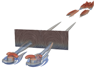
The numerical set-ups of the boundary layer study with embedded corotating and counter-rotating cylindrical roughness elements are illustrated in figures 1(a) and 1(b), respectively. The roughness elements with height  $k$ and diameter $D$ are placed at the location $x_k$ from the flat plate leading edge, under zero-pressure gradient in the streamwise direction. At this station, the non-dimensional displacement thickness is $\delta ^*/k = 0.6883$. A roughness pair consists of two rotating roughness elements with spacing $\lambda$, as shown in figure 1. The spanwise spacing between roughness pairs is $\varLambda$. The origin of the local $x,y,z$ coordinate system is placed at the location of the roughness element $x_k$ for the corotating case and is placed at the centre of the roughness pair for the counter-rotating case. Hereafter, all length scales are non-dimensionalized by the dimensional roughness height $\bar {k}$. The incoming free stream velocity is $u_\infty$. Depending on the rotation sense of the roughness pair, different types of downstream streaks are created. For the corotating roughness case, the generated downstream vortices rotate in the same direction, which will counteract the momentum exchange effect of neighbouring vortices. In contrast, this momentum exchange effect is intensified in the case of counter-rotating roughness elements. The strength of the generated downstream vortices depends on the rotation velocity of the roughness elements. This can be expressed in non-dimensional form by the ratio of the tangential velocity induced by the cylindrical roughness element to the incoming local velocity at its top, i.e.
 \begin{equation} \varOmega_u= \frac{\varOmega D}{2u(k)}, \end{equation}
where  $\varOmega$ is the angular velocity of the cylinder and $u(k)$ is the unperturbed Blasius velocity at the upper edge of the cylinder.

Figure 1. Numerical set-up of rotating roughness elements embedded into a flat-plate boundary layer. High- and low-momentum flow induced by streamwise vortices are coloured in red and blue, respectively. (a) Corotating roughness elements; (b) counter-rotating roughness elements.
The configurations considered in the present study are summarized in table 1. The counter-rotating cases C1, C2 and C4 differ by their aspect ratio  $\eta$, the spacings ( $\lambda$, $\varLambda$) and the positive and negative rotation sense as indicated in the table. In the positive counter-rotating case, a high-momentum fluid area is induced in the middle of the roughness pair. In the negative rotation case, a low momentum fluid is induced in the middle of the roughness pair. The roughness spacings ( $\lambda , \varLambda$) in case C1 follow the case C01 from Siconolfi et al. (Reference Siconolfi, Camarri and Fransson2015), which demonstrated an effective delay of laminar–turbulent transition induced by TS waves. The roughness elements in the corotating case C3 are equally spaced, to simulate a regular roughness array. A small and a moderate rotation rate are considered for the counter-rotating case, i.e. $\varOmega _u=0.2$ and $0.46$, respectively. The static roughness array case, i.e. $\varOmega _u=0$ in case C3, is taken as reference.
Table 1. Parameters of simulation, non-dimensionalized with respect to roughness height  $\bar {k}=0.01\ \textrm {m}$ and free stream velocity $\bar {u}_\infty =0.937\ \textrm {m}\ \textrm {s}^{-1}$.
 $^{a}+$: rotation direction with high-momentum creation in the centre. $^{b}-$: rotation direction with low-momentum creation in the centre.
2.2. Base flow computation
In LST, the flow quantities  $\boldsymbol {q}(\boldsymbol {x},t)= \lbrace u,v,w,p \rbrace (\boldsymbol {x},t)$ are split into a steady baseflow $\boldsymbol {q_0}(\boldsymbol {x})$ and an unsteady perturbation $\boldsymbol {q'}(\boldsymbol {x},t)$ similar to the Reynolds decomposition. In this study, the steady baseflows have been computed with the method of selective frequency damping (SFD) (Åkervik et al. Reference Åkervik, Brandt, Henningson, Hœpffner, Marxen and Schlatter2006). In the SFD approach, a filtered state $\tilde {\boldsymbol {u}}$ is introduced and its evolutionary equation is solved together with the Navier–Stokes equations. The following non-dimensional governing equations are obtained:
 \begin{gather} \boldsymbol{\nabla}\boldsymbol{\cdot} \boldsymbol{u} =0, \end{gather}
 \begin{gather}\frac{\partial \boldsymbol{u}}{\partial t} + (\boldsymbol{u}\boldsymbol{\cdot}\boldsymbol{\nabla})\boldsymbol{u} ={-}\boldsymbol{\nabla} p +\frac{1}{Re_k}\Delta \boldsymbol{u} - \chi (\boldsymbol{u} - \tilde{\boldsymbol{u}}), \end{gather}
 \begin{gather}\frac{\partial \tilde{\boldsymbol{u}}}{ \partial t} = \omega_c (\boldsymbol{u} - \tilde{\boldsymbol{u}}), \end{gather}
where  $Re_k =\bar {u}_\infty \bar {k} / \bar {\nu }$ is the Reynolds number based on free stream velocity, $\omega _c$ is the filter cutoff circular frequency and $\chi$ is the feedback control coefficient. An overbar denotes dimensional values, hence $t=\bar {t} \bar {u}_\infty / \bar {k}$ and $p=\bar {p}/(\bar {\rho } \bar {u}^2)$. The additional forcing term on the right-hand side of the momentum equation works as a temporal low-pass filter. From theoretical analysis it is known that the cutoff frequency $\omega _c$ should be lower than the frequency of the lowest instability, while the feedback control coefficient $\chi$ should be higher than the growth rate of that instability (Åkervik et al. Reference Åkervik, Brandt, Henningson, Hœpffner, Marxen and Schlatter2006).
The above governing equations are implemented and solved with the open source OpenFOAM solver icoFoam, which solves the incompressible Navier–Stokes equations using the pressure implicit with splitting of operators (known as PISO) algorithm. The pressure equation is solved by the geometric algebraic multigrid (known as GAMG) solver and the velocity equation by the preconditioned biconjugate gradient (known as PBiCG) solver. The integration domain has a streamwise extent of  $L_x = 320$ ( $-20\sim x \sim 300$) and a wall-normal extent of $L_y =40$. The spanwise extent $L_z$ is determined by the roughness pair spacing $\varLambda$, as given in table 1. For computational efficiency (Shrestha & Candler Reference Shrestha and Candler2019), the Blasius boundary layer velocity profile is prescribed to the inlet according to the distance from the leading edge of the flat plate. No-slip wall boundary conditions are applied at the bottom wall. The cylinder can be rotated with constant $\varOmega$ about its vertical axis leading to a constant tangential velocity $u_w=\varOmega D /2$ at the cylinder wall. The following direction mixed boundary condition is imposed at the top of the integration domain:
 \begin{gather} \frac{u}{u_\infty} = 1 , \end{gather}
 \begin{gather}\frac{\partial v}{\partial n} = \frac{\partial w}{\partial n} = 0. \end{gather}
Here,  $n$ denotes surface norm. At the outlet, any possible reflection is eliminated by using the following advective boundary condition together with a sponge zone with gradually increasing damping strength towards the outlet:
 \begin{equation} \frac{\textrm{D} q}{\textrm{D}t} = \frac{\partial q}{\partial t} + \boldsymbol{u} \boldsymbol{\cdot} \boldsymbol{\nabla} q = 0. \end{equation}
 A structured grid is used to discretize the above governing partial differential equations. Following the grid convergence study in Wu & Rist (Reference Wu and Rist2020), 80 grid points are used to resolve the boundary layer, which is sufficient for a laminar flow computation. An expansion (with ratio  $r=1.02 \text {--} 1.2$) of the grid spacing toward the far field is applied to reduce the total grid points, and 300 equidistant grid points in the circumferential direction are used around the cylinder.
2.3. Biglobal linear stability analysis
In this paper, the instability of the boundary layer is studied with the so-called biglobal LST (Theofilis Reference Theofilis2011). With this method, the asymptotic behaviour of infinitesimally small 3-D perturbations superimposed on a 2-D base flow can be analysed. Transient growth is not considered here. The analysed base flow is assumed to be parallel in  $x$, i.e. $\partial \boldsymbol {q_0}/ \partial x \approx 0$. The perturbations $\boldsymbol {q'}(\boldsymbol {x},t)$ are modelled by the normal mode ansatz,
 \begin{equation} \boldsymbol{q}^{\prime}(x, y,z,t) =\boldsymbol{\hat{q}}(y,z)\exp({\textrm{i}(\alpha x-\omega t)}) +\textrm{c.c.}, \end{equation}
where  $\boldsymbol {\hat {q}}$ is a 2-D complex amplitude function, $\alpha$ the real streamwise wavenumber, $\omega =\omega _r +\textrm {i}\omega _i$ the complex frequency, and c.c. the complex conjugate. The real part of the eigenvalue $\omega _r$ corresponds to the angular frequency of the eigenmode/instability, while the imaginary part $\omega _i$ determines its exponential growth. The instability wave amplifies in case of positive $\omega _i$ and it decays with negative $\omega _i$. Inserting (2.8) into the linearized Navier–Stokes equations and recasting the coefficients results in the following generalized eigenvalue problem for temporal stability analysis:
 \begin{equation} L\hat{\boldsymbol{q}}=\omega M\hat{\boldsymbol{q}}, \end{equation}
where  $L$ and $M$ are the coefficient matrices, given in Appendix A.
The generalized eigenvalue problem is discretized on a  $y$–
$y$– $z$ plane at consecutive streamwise stations $x=\textrm {constant}$, which are interpolated from the numerical simulation with a cubic spline. Equation (2.9) is discretized by the Fourier spectral method in the wall-normal direction and the summation-by-parts method (Mattsson & Nordström Reference Mattsson and Nordström2004) in the spanwise direction. The grid is clustered toward the wall following the mapping successfully used by Staudenmeyer, Schnoebel & Rist (Reference Staudenmeyer, Schnoebel and Rist2019) for streamwise corner-flow instability with the same eigenvalue solver,
 \begin{equation} y= \frac{-\tanh\left(-(b_1-b_2)\dfrac{\bar{y}}{y_{max}}-b_2\right) - \tanh b_2}{\tanh b_1 -\tanh b_2} y_{max}, \end{equation}
with the coefficients  $b_1 =0.5$, $b_2=-1.2$ and the cutoff wall-normal extent $y_{max} \approx 6 \text {--} 10$. A grid convergence study has been performed to identify the necessary discretization: $N_y = 65$, and $N_z=110$. At the wall surface, the boundary condition for (2.9) is $\boldsymbol {\hat {q}} = 0$. The von Neumann boundary condition $\partial \boldsymbol {\hat {q}} / \partial y = 0$ is specified at the top boundary, and for the spanwise boundary a periodic boundary condition is used. The ARPACK (Lehoucq, Sorensen & Yang Reference Lehoucq, Sorensen and Yang1998) routine which uses an implicitly restarted Arnoldi method is employed to solve the generalized eigenvalue problem, (2.9). The solution procedure is implemented in Python code, the validation of which has been performed by comparing the TS-wave amplitude and its growth rate with numerical simulation (Wu & Rist Reference Wu and Rist2020). Another successful application of the code can be found in Puckert, Wu & Rist (Reference Puckert, Wu and Rist2020).
2.4. PKE analysis
For an analysis of the instability mechanisms, the PKE analysis following Cossu & Brandt (Reference Cossu and Brandt2004) is used. The basic idea is to derive the evolution equation for the PKE  $e'=(u'^{2}+v'^{2}+w'^{2})/2$ under the assumption of periodic waves in the streamwise direction. By integrating the PKE in the $y$–
$y$– $z$ plane and over a wavelength in the $x$ direction, the following reduced Reynolds–Orr equation is obtained:
 \begin{equation} \frac{\partial E}{\partial t}=T_{y}+T_{z}-D, \end{equation}
where  $E$ is the total PKE and $D$ the viscous dissipation energy. Here $T_{y}$ and $T_{z}$ are the production energies from the interaction of Reynolds stresses $u'v'$ and $u'w'$ with wall-normal shear $\partial u_0/\partial y$ and spanwise shear $\partial u_0/\partial z$, respectively. The above identity means that the temporal growth rate of the instability mode is composed of three parts: the wall-normal, the spanwise production and the viscous dissipation. Based on the normal-mode ansatz of the perturbation $\boldsymbol {q'}$, the perturbation energy balance terms can be expressed in the form $(E,D,T_{y},T_{z})=(\hat {E},\hat {D},\hat {T}_{y},\hat {T}_{z})\,\textrm {e}^{2\omega _{i}t}$, where $\omega _i$ is the temporal growth rate from the normal mode ansatz in (2.8). Substituting this expression back into (2.11), leads to
 \begin{equation} {\omega_i=\frac{\hat{T}_{y}}{2\hat{E}}+\frac{\hat{T}_{z}}{2\hat{E}}-\frac{\hat{D}}{2\hat{E}}}, \end{equation}
where the terms on the right-hand side are as follows:
 \begin{gather} \hat{E} = \frac{1}{\varLambda}\int_{-\varLambda/2}^{\varLambda/2}\int_0^{y_{max}} \hat{e} \,\textrm{d}y\,\textrm{d}z, \end{gather}
 \begin{gather}\hat{T}_y = \frac{1}{\varLambda}\int_{-\varLambda/2}^{\varLambda/2}\int_0^{y_{max}} -\hat{\tau}_{xy}\frac{\partial u_0}{\partial y} \,\textrm{d}y\,\textrm{d}z, \end{gather}
 \begin{gather}\hat{T}_z = \frac{1}{\varLambda}\int_{-\varLambda/2}^{\varLambda/2}\int_0^{y_{max}} -\hat{\tau}_{xz} \frac{\partial u_0}{\partial z} \,\textrm{d}y\,\textrm{d}z, \end{gather}
 \begin{gather}\hat{D} = \frac{1}{\varLambda Re_k} \int_{-\varLambda/2}^{\varLambda/2}\int_0^{y_{max}} \hat{d} \,\textrm{d}y\,\textrm{d}z . \end{gather}
Here  $\hat {\tau }_{xy}, \hat {\tau }_{xz}$ denote wall-normal and spanwise Reynolds stress components calculated from the instability wave amplitude function, respectively, and $\hat {d}$ is the viscous dissipation calculated from the perturbation vorticity vector.
3. Results and discussion
3.1. Base flow
In figure 2, vortex structures induced by an isolated static and an isolated rotating cylindrical roughness element are illustrated by means of  $\lambda _2$ isosurfaces (Jeong & Hussain Reference Jeong and Hussain1995). This serves the purpose of illustrating the influence of rotation on the vortex structure. While two pairs of equally strong counter-rotating vortices are excited by the static roughness element, the rotating case shows differences with respect to the symmetry and relative strength of its vortices. The naming convention for the induced vortices follows that of Groskopf & Kloker (Reference Groskopf and Kloker2016), due to the similarity of the generated vortex structure between the rotating roughness element and their oblique roughness element. For the typical static roughness element (cf. figure 2a), spanwise vorticity is created in front of the roughness element as the boundary layer is blocked by it. The vorticity rolls up and wraps around the cylindrical roughness element, and then develops into a pair of HV legs in the streamwise direction. Another weaker pair of IV is generated directly behind the roughness element, beginning from the downstream reverse flow region. For the rotating case, the vortices are no longer symmetric, see figure 2(b). Instead, one IV gets strengthened and becomes the DIV in the downstream area. On the other hand, the other IV is weakened and rotates around the DIV, hence named SIV. The HV pair is also weakened and vanishes in the near-wake region. The formation of the DIV is well illustrated in figure 3, and can be summarized as follows.
(i) The rotating cylinder accelerates the flow on one side, reduces the reverse flow region and pushes it towards the decelerated side such that a symmetric HV is no longer possible.
(ii) Since the cylinder rotates at a constant angular velocity, the acceleration effect is stronger close to the wall, thus forming a locally accelerated flow, see figure 3(a). Depending on the strength of the accelerated flow, an additional reverse flow can be induced behind it.
(iii) This accelerated flow meets with the high-speed flow on the decelerated side, therefore creating the strong DIV.

Figure 2. Vortex visualization for isolated roughness element ( $Re_{kk}=465.8, \eta =1, x_k=99.2$) by means of $\lambda _2=-15$, coloured by streamwise velocity $u$: (a) static case, $\varOmega _u=0$; (b) rotating case, $\varOmega _u=0.46$. The abbreviations used are: horseshoe vortex (HV); inner vortex (IV); dominating inner vortex (DIV); secondary inner vortex (SIV).

Figure 3. Flow field visualized by line integral convolution (known as LIC) (Cabral & Leedom Reference Cabral and Leedom1993; Loring, Karimabadi & Rortershteyn Reference Loring, Karimabadi and Rortershteyn2014) for rotating case ( $Re_{kk}=465.8, \eta =1, x_k=99.2, \varOmega _u=0.46$), coloured by streamwise velocity $u$. The yellow curve marks the reverse flow region. $(a)\ y = 0.15;\ (b)\ y = 0.4;\ (c)\ y = 1.02.$
The single leg of the streamwise DIV is stronger compared with those of the HV in the static case, thus it is more effective in pulling high-speed fluid towards the wall and pushing low-speed fluid to the outer region of the boundary layer. In other words, the lift-up effect (Landahl Reference Landahl1990) is stronger in the rotating roughness case compared with its static counterpart, therefore it is able to create stronger streamwise streaks. The locally accelerated flow at the bottom also creates a slight cross-flow in the downstream wake of the cylinder.
It turns out that the characteristics of the DIV created by the isolated roughness element can be used to control velocity streaks. It is the purpose of this paper to investigate the linear stability property of a boundary layer with different combinations of rotating roughness elements, i.e. corotating roughness arrays and counter-rotating roughness pairs. Figure 4 presents slices of the steady base flow obtained from the SFD solver with the identified vortices, high shear regions (by means of  $I_2=\textrm {constant}$, see Meyer (Reference Meyer2003)) and the velocity gradients ( $\partial u/ \partial y$ and $\partial u/ \partial z$). Two slices are shown for each case, one at $x =5$ (in the two top rows) the other at $x =40$ (in the two lower rows). In the near-wake region ( $x =5$), the location of the HVs on the sides of the DIV is observable for all cases. Since the DIV rotates in a clockwise sense (see figure 4c for instance), a stronger high velocity streak is created on its right-hand side and a stronger low velocity streak is created on its left-hand side compared with its static counterpart. This feature is more obvious at the downstream slice, i.e. at $x =40$. This alternating high–low–high velocity streak pattern would attenuate the strength of the DIV, if the neighbouring corotating roughness elements were too close to each other. Contrary to this attenuation effect, the counter-rotating roughness pair intensifies either the high-speed or the low-speed velocity streak, depending on the rotation direction. In figure 4(a), the counter-rotating roughness pair rotates in the direction which intensifies the high-speed velocity streak and the low-speed velocity streaks on the side are dissipated by viscosity. It is typical for streaky flow to have a high-shear region above the low-speed velocity streak. At slice $x =5$, it is obvious that a high-shear region ( $I_2=-450$) composed of wall-normal ( $\partial u / \partial y$) and spanwise ( $\partial u / \partial z$) terms exists above the DIV. This structure belongs to an inflectional velocity profile, where inviscid inflectional instability could be expected. At slice $x =40$, this high-shear region with inflection point still exists for corotating case C3 due to the long-living DIV, while for the counter-rotating case C1 only the intensified high-speed streak persists. The latter happens to be a preferable velocity profile with respect to the stabilization of TS-waves (Siconolfi et al. Reference Siconolfi, Camarri and Fransson2015).

Figure 4. Presentation of streamwise baseflow: (a) counter-rotating case C1; (b) counter-rotating case C2; (c) corotating case C3; (d) corotating case C4. The thin solid lines are isolines of  $u =0.1\text {--} 0.95$; thick black lines visualize vortex cores by means of $\lambda _2=-5$; thick cyan lines visualize shear regions by means of $I_2 = -450$. In the first and second rows $x =5$ and in the third and fourth rows $x =40$. In the first and third rows $\partial u / \partial y$ and in the second and fourth rows $\partial u / \partial z$. $(a)\ C1, \varOmega_{u} = 0.46;\ (b)\ C2, \varOmega_{u} = 0.2;\ (c)\ C3, \varOmega_{u} = 0.46;\ (d)\ C4, \varOmega_{u} = 0.2$.
Figure 5 shows the streamwise evolution of the velocity gradient maxima in  $y$–
$y$– $z$ planes for all three types of streaky flows by corotation (case C3), positive counter-rotation (case C2) and negative counter-rotation (case C4) of the roughness elements. It is clear that the primary components of shear are the $\partial u / \partial y$ and $\partial u / \partial z$ terms in both static and rotating cases. The other terms are several magnitudes lower. Comparing figure 5(b) with figure 5(a), it is clear that the rotation effect not only promotes these two terms, but also slightly increases the $\partial w / \partial y$ and $\partial v / \partial z$ terms. However, the streamwise gradient terms $\partial / \partial x$ remain negligibly low except for the very short near-wake region ( $x <5$), i.e. the reverse-flow region. This observation validates use of the parallel flow assumption as in Groskopf & Kloker (Reference Groskopf and Kloker2016), for instance. Since the production of the PKE is proportional to the shear magnitude, it can be inferred that the associated instability mode is fundamentally determined by the wall-normal and spanwise productions which justifies using the reduced Reynolds–Orr equation, i.e. (2.11) for perturbation energy analysis.

Figure 5. Evolution of baseflow gradient maxima in  $y$–
$y$– $z$ planes: (a) C3, $\varOmega _u=0$; (b) C3, $\varOmega _u=0.46$; (c) C2, $\varOmega _u=0.46$; (d) C4, $\varOmega _u=0.46$.
To quantify the amplitude of velocity streaks, the following definition of Groskopf & Kloker (Reference Groskopf and Kloker2016) is used:
 \begin{equation} u_{st}(x) = \tfrac{1}{2}\left(\max_{yz}[u(x,y,z)-\langle u \rangle(x,y)] -\min_{yz}[u(x,y,z)-\langle u \rangle(x,y)]\right), \end{equation}
where  $\langle u \rangle$ is the spanwise mean value, which represents the 3-D baseflow deformation caused by the low- and high-speed streaks. In figure 6, the streamwise evolution of the streak amplitudes for the cases from table 1 are compared. A rapid growth of the streak at the roughness element ( $x=0$) can be observed. A subsequent transient growth of the streak amplitude begins from $x \approx 30$ for case C1 with $\varOmega _u=0.1$. With increasing rotation rate, this starting position moves forward until $x \approx 5$. Such tendency is also observed for other cases, especially case C3. For cases C1 and C3 with $\varOmega _u=0.46$, the streaks reach a peak ( $u_{st}=0.32$) at around $x \approx 55$ and thereafter decay gradually. With increasing rotation rate, the streak amplitudes of these two cases evolve similarly with an almost constant offset. The streak evolution for cases C2 and C4 exhibit some differences. Here, the velocity streak maxima occur closer to the roughness for lower rotation rates ( $\varOmega _u=0.2$). For higher rotation rate ( $\varOmega _u=0.46$), an additional peak can be observed at $x \approx 100$ for case C4 and $x \approx 200$ for case C2. Both postpone the decay of the streaks leading to a higher streak amplitude.

Figure 6. Streamwise evolution of velocity streak amplitudes.
3.2. Linear stability analysis
Linear stability analysis is performed at the same streamwise location  $x = 100$, where the base flow is quasi-parallel, for all cases presented in table 1. Two types of modes are identified, the viscous TS-like mode and the inviscid inflectional mode, both clearly shown in figure 7 for four cases. The TS-like mode contains a 3-D distortion relative to the 2-D TS mode of the Blasius boundary layer, due to the influence of the velocity streaks. The TS-like mode's amplitude maximum is located close to the wall and the mode travels downstream with a phase speed $c_{ph}= \omega _r/\alpha \approx 0.3 \text {--} 0.4$. Due to the influence of the streaks, the TS-like mode exhibits alternating signs in spanwise direction, as shown in figures 7(a) and 7(b). This amplitude modulation is mainly induced by the low-speed streak, which is clearest in figure 7(b) at $z = \pm 2$. The inviscid inflectional modes in figures 7(c) and 7(d) are found to reside on the high-shear region which is identified by the $I_2$ criterion. Since the high-shear region is induced by the roughness element, the mode is hereafter called the roughness mode. The roughness modes display a primary structure in the high-shear region and secondary structures which are in antiphase to the primary at the sides of the high-speed streaks. The shown roughness modal structures for cases C2 and C4 are similar to each other. If the two low-speed regions in C2 move closer to each other, the shown modal structures would coalesce to the shape of case C4. The amplitude of the $\hat {v},\hat {w}$ components of the shown TS-like mode is quite small compared with the corresponding $\hat {u}$ components, whereas the $\hat {v}$ component of the shown roughness mode is similar to the amplitude of the $\hat {u}$ component. What is more, the $\hat {u},\hat {v}$ components always appear in antiphase. It is also to be noted that the typical symmetric sense of the roughness modes as found in the static roughness case is lost, the mode shown in this paper is always the most amplified one.

Figure 7. Real part of mode component  $\hat {u}$ (top), $\hat {v}$ (middle), $\hat {w}$ (bottom) of the typical TS-like mode (a,b) with $\alpha = 0.35$ and the roughness mode (c,d) with $\alpha = 1$ extracted at $x =100$. The thick red line marks phase speed $c_{ph}$ of the corresponding mode. The thin solid lines are isolines of $u =0.1\text {--} 0.95$. The thick cyan solid lines visualize shear regions by means of $I_2 = -180$. The $\varOmega _u$ for each case: (a) case C3, $\varOmega _u=0.2$; (b) case C1, $\varOmega _u=0.2$; (c) case C2, $\varOmega _u=0.46$; (d) case C4, $\varOmega _u=0.46$.
The effect of different streaks on the boundary layer stability is studied by computing the eigenvalue problem (2.9) at streamwise location  $x = 100$ for a set of wavenumbers $\alpha$. The temporal amplification rate $\omega _i$ and corresponding phase velocity $c_{ph}$ are shown in figure 8 for both TS-like mode and roughness mode. The TS mode of the undisturbed Blasius boundary layer, which is slightly amplified around $\alpha =0.35$, is evaluated at the same streamwise location for reference. The two types of modes differ by their phase velocity $c_{ph}$, such that the TS-like mode travels at a lower speed ( $c_{ph} \approx 0.3 \text {--} 0.4$) than the roughness mode ( $c_{ph} \approx 0.6 \text {--} 0.8$). The identified phase speed for the roughness mode is similar to the results of Di Giovanni & Stemmer (Reference Di Giovanni and Stemmer2018), who found that a roughness-induced mode travels at $c_{ph} = 0.68u_\infty$ in a hypersonic boundary layer. For the TS-like mode, all streaks are capable of attenuating the TS-like mode except for the case C4 with high rotation rate ( $\varOmega _u=0.46$), where the roughness mode gets mostly amplified with a relatively high amplification rate. Only the roughness modes for cases C1 and C3 with low rotation rate ( $\varOmega _u=0.2$) remain damped. While at lower rotation rate ( $\varOmega _u=0.2$), the amplified mode peaks at a wavenumber around $\alpha = 0.5$, the roughness mode with higher rotation rate ( $\varOmega _u=0.46$) peaks at a larger wavenumber around $\alpha = 1.0$. It is also found that the amplification rate for roughness modes increases with rotation rate. At the same time, the most amplified wavenumber moves to higher values. However, among all cases, the TS-wave attenuation effect is only observed to increase with increasing rotation rate in configuration C1, i.e. positive counter-rotating roughness elements. Such tendency is not that obvious for other cases. This indicates that only thin roughness elements with low rotation rate are suitable for boundary layer instability attenuation or possible transition delay, otherwise the additional roughness mode is always a threat leading to a fast-growing inflectional instability.

Figure 8. Growth rate  $\omega _i$ and phase velocity $c_{ph}$ at slice $x =100$: (a,c) TS-like mode; (b,d) roughness mode.
In figure 9, temporal stability diagrams obtained by tracking eigenmodes in the  $(\alpha , x)$-space are presented. The TS-like modes of case C1 with $\varOmega _u=0.1$ and $0.2$ are compared with the TS mode flat-plate boundary layer in the upper row. The $x$ position corresponding to the critical Reynolds number for the unperturbed TS-mode is at $x =85$ with wavenumber $\alpha = 0.37$. With a slight rotation ( $\varOmega _u=0.1$), the critical position moves forward to $x =38$ and the wavenumber reduces to $\alpha = 0.34$. However, the overall amplification rate $\omega _i$ is greatly reduced, as the maximum is decreased by $40\,\%$ from $2\times 10^{-3}$ to $1.2\times 10^{-3}$. With further increase of the rotation rate to $\varOmega _u=0.2$ the TS-like mode is fully damped in the studied streamwise range. The shown contour levels are hence all negative in figure 9(c). The TS-like mode for even higher rotation rate $\varOmega _u=0.46$, which is not shown here for convenience, is also fully damped in the studied streamwise range.

Figure 9. Temporal stability diagrams of TS mode (a), TS-like mode (b–c) and roughness mode (d–f): (b) case C1,  $\varOmega _u=0.1$; (c) case C1, $\varOmega _u=0.2$; (d) case C3, $\varOmega _u=0$; (e) case C2, $\varOmega _u=0.2$; (f) case C2, $\varOmega _u=0.46$. The thick solid lines mark the TS mode's neutral curve for comparison.
The stability diagram of the most amplified roughness mode for case C2 is compared with the static roughness array case from C3 in the lower row of figure 9. The roughness mode seems to be mainly amplified directly behind the roughness element. However, as indicated in the velocity gradients (cf. figure 5), the parallel flow assumption most probably fails in the direct vicinity of the roughness wake, this must be treated with caution. Hence, the roughness mode is only tracked from  $x =5$ downstream where the initial transients from figure 5 have decayed. Compared with the TS-like mode, the roughness mode is amplified more strongly and within a broader range of wavenumbers. Since the roughness elements impose an abrupt geometric discontinuity to the boundary layer flow, extreme high shear can be found in the near-wake region, where multiple unstable modes can be found in the LST analysis. While the amplified region of the static reference case only extends to $x =25$, the rotation effect extends the amplified region to the full streamwise region for both cases. Besides, there are three notable features in the stability diagram of the roughness mode. The first is that the most amplified instability moves to a higher wavenumber. The second is that the highly amplified near-wake region moves closer to the roughness elements. The third feature is that a second peak appears at $x =60$ for higher rotation rate in figure 9(f). In fact, this peak already emerges at $x =100$ for the case with $\varOmega _u=0.2$ in figure 9(e). The rotation effect moves the second peak to higher wavenumber and forward to the roughness elements as well. This observation is consistent with the observation of a local velocity streak amplitude maximum in figure 6(b).
3.3. Instability mechanisms
Perturbation kinetic energy analysis is performed to get a deeper understanding of the linear instability mechanisms. Results are shown in figure 10. The integral energy terms ( $\hat {T}_y, \hat {T}_z$) are normalized with respect to their corresponding dissipation terms $\hat {D}$. In case C1, the amplified reference TS mode is also plotted together with the TS-like mode. As the TS mode is 2-D, the spanwise production term $\hat {T}_z$ is negligibly small. Since the wall-normal production term $\hat {T}_y$ exceeds the dissipation term $\hat {D}$, the TS mode is amplified as a result of extracting energy from the baseflow. At very low rotation rate ( $\varOmega _u=0.1$), the $\hat {T}_y$ term is slightly lower than that of the TS mode and the $\hat {T}_z$ term is found to be negative. This negative spanwise production term is considered to be the responsible mechanism for TS-wave attenuation and transition delay with static roughness elements (Cossu & Brandt Reference Cossu and Brandt2004; Fransson et al. Reference Fransson, Talamelli, Brandt and Cossu2006). The reference case with static roughness ( $\varOmega _u=0$) is plotted with C3 as well. With this set-up, the spanwise production energy is also found to be negative, but it is not strong enough to surpass the wall-normal production energy. With increasing $\varOmega _u$, the negative spanwise production term $\hat {T}_z$ becomes positive in case C1. On the other hand, the wall-normal production term $\hat {T}_y$ reduces dramatically. Therefore, the sum of production terms becomes smaller than the dissipation term, resulting in an overall attenuation of the TS-like mode. Such mechanisms, i.e. reduction of wall-normal production and amplification of spanwise production perturbation energy, are also observed for the TS-like mode in cases C2, C3 and C4. In cases C2 and C4, the wall-normal production term is even reduced to a negative value at high rotation rate ( $\varOmega _u=0.46$), although the negative side is the overshoot of the spanwise production term over the dissipation, see case C4 with $\varOmega _u=0.46$ in figures 10 and 8.

Figure 10. Normalized PKE production and dissipation components. Mode evaluated at slice  $x =100$ with $\alpha = 0.35$ for TS-like mode and $\alpha = 0.5$ for roughness mode ( $\alpha = 1$ for roughness mode C1, C3, C4 with $\varOmega _u=0.46$).
Perturbation kinetic energy analysis results for the roughness mode are shown in the right column of figure 10. In case C1, both production terms are relatively low when the rotation rate is small ( $\varOmega _u=0.1, 0.2$). However, the wall-normal term $\hat {T}_y$ rises significantly at high rotation rate ( $\varOmega _u=0.46$). Such notable increase of the wall-normal production term is also evident for all other cases, especially in cases C2 and C4 where the wall-normal productions rise up to four and six times the dissipation term, respectively. Although the increase of $\hat {T}_y$ in case C3 is relatively small, it still reaches 1.5 times the dissipation term. In addition, the spanwise production term $\hat {T}_z$ is also increased to 1.8 times the dissipation term. This unique feature of the roughness mode is due to the fact that case C3 is the only corotation set-up in which both wall-normal shear $\partial u / \partial y$ and spanwise shear $\partial u / \partial z$ are significantly increased. To conclude, the roughness mode can be destabilized by the streaks induced by rotating roughness elements and the according destabilization effect is much more significant than the stabilization effect of the TS-like mode, in agreement with the amplification rates in figure 8. In § 3.4 we shall investigate whether this destabilization leads to immediate laminar–turbulent transition at the roughness elements or not.
The above mechanisms can be further explained by examining the spatial distribution of the PKE terms for each type of mode. Contour plots of the PKE terms for the TS-like mode from case C1 are shown in figure 11. Both  $\hat {T}_y$ and $\hat {T}_z$ are the product of Reynolds shear stresses ( $\hat {\tau }_{xy}$, $\hat {\tau }_{xz}$) and baseflow velocity gradients ( $\partial u/ \partial y$, $\partial u/ \partial z$), both of which can be positive or negative. The corresponding signs of the involved Reynolds shear stresses and the baseflow velocity gradients determine the sign of the PKE production. As mentioned above, the spanwise production term for the TS mode is zero, since there is no spanwise velocity gradient. However, neither the spanwise velocity gradient nor the spanwise Reynolds shear stress is zero in streaky flows, the multiplication of the two terms results in unavoidable non-negative spanwise production. Figure 11(a) shows the spatial distribution of the PKE terms for case C1 with low rotation rate ( $\varOmega _u=0.1$), which is a case closest to the result of the TS mode. As already explained, the spanwise production term for the TS mode is zero and the wall-normal production is positive throughout the boundary layer. Due to the effect of the velocity streaks, the otherwise constant sign of the wall-normal production is broken, see the top subpanels of figure 11. The positive and negative production terms cancel each other in the spanwise mean, leading to the reduction of the wall-normal production $\hat {T}_y$ for the TS-like mode as shown in figure 10. The spanwise production is also composed of parts with opposite signs, which inhibit the growth of the integral value as rotation rate increases. This explains why the spanwise production $\hat {T}_z$ of the TS-like mode for case C1 remains almost unchanged for $\varOmega _u=0.1$ and $\varOmega _u=0.2$ in figure 10. With higher rotation rate ( $\varOmega _u=0.46$), the negative parts of the spanwise production become negligibly low, making the positive parts dominant, which explains the rapid rise of the integral value. The rise of the spanwise production can be so strong that it again destabilizes the TS-mode, see the TS-like mode of case C4 in figures 10 and 8.

Figure 11. Perturbation production of wall-normal  $\hat {T}_y$ (top), spanwise $\hat {T}_z$ (middle) and dissipation $\hat {D}$ (bottom) terms of typical TS-like mode for case C1 with (a) $\varOmega _u=0.1$; (b) $\varOmega _u=0.2$; (c) $\varOmega _u=0.46$. Spatial distributions are normalized by local maxima. The thin solid lines are isolines of $u =0.1\text {--} 0.95$.
The spatial distributions of the PKE terms for the roughness mode of cases C2 and C3 are shown in figure 12. For the inflectional instability, the productions are mostly concentrated above the low-speed streak where inflection points can be found. The negative part of the wall-normal production is lower compared with the spanwise production for the case shown. As rotation rate increases, the wall-normal production intensifies and results in a higher integral value. However, the robust negative part in the spanwise production restricts the rise of the integral value. This explains the behaviour of spanwise production  $\hat {T}_z$ for the roughness mode in figure 10. Nevertheless, the high wall-normal production has already destabilized the roughness mode. The rise of $\hat {T}_z$ in case C3 is due to the unique feature of the velocity streak induced by the corotating roughness elements, that both wall-normal and spanwise production are intensified, see figures 12(c) and 12(d).

Figure 12. Perturbation production of wall-normal  $\hat {T}_y$ (top), spanwise $\hat {T}_z$ (middle) and dissipation $\hat {D}$ (bottom) terms of roughness mode for case C2 (a,b) and case C3 (c,d) with (a) case C2, $\varOmega _u=0.2$; (b) case C2, $\varOmega _u=0.46$; (c) case C3, $\varOmega _u=0.2$; (d) case C3, $\varOmega _u=0.46$. Spatial distributions are normalized by local maxima. The thin solid lines are isolines of $u =0.1\text {--} 0.95$.
3.4. Exclusion of a possible bypass transition
The results presented so far have identified two opposing effects: stabilization of TS-modes and destabilization of roughness modes. Especially, the latter appears to be strongest towards the roughness elements where the local stability analysis is no longer valid. Therefore, in order to exclude both, a possible bypass transition and a possible global instability, a DNS is conducted for case C2 with pairs of counter-rotating roughness elements and  $\varOmega _u = 0.46$, for which the previous LST predicts that the amplification rate of the roughness mode is 100 times larger than that of the T–S mode. The steady-state base flow is used as the initial field, and the nonlinear Navier–Stokes equations are marched in time. A blowing–suction disturbance strip is placed ahead of the roughness elements from $x =-11$ to $-10$ to trigger disturbances with a broad spectrum. The wall-normal velocity component mapped to the wall within the disturbance strip is specified as (cf. Kurz & Kloker Reference Kurz and Kloker2016)
 \begin{equation} v(x^*,y^*=0,z^*,t) = \hat{A} \sin({\rm \pi} x^*)\exp({-({\rm \pi} x^*)^2/\sqrt{2}}) \frac{1}{50} \sum_{n=1}^{50}\cos(2{\rm \pi}\, f_0nt), \quad x^* \in [{-}1;1], \end{equation}
where  $\hat {A}$ is the amplitude and $f_0=0.25\ \textrm {Hz}$ is the fundamental frequency. Frequencies with $n=1\text {--}50$ are superimposed to produce a periodic pulse disturbance which will excite a broad spectrum of instability waves. The frequencies of this spectrum are chosen such that its lower part covers the dominant TS-modes and its higher part covers the dominant roughness modes. Their different frequencies can be inferred from their different wavenumbers in figure 9. In addition, the spatial distribution and temporal modulation of the disturbance strip is switched on and switched off after four fundamental periods $T_0=1/\,f_0$, as shown by the dashed envelope curve together with a snapshot of the disturbance field $u'=u-u_0$ at wall distance ( $y=1$) in figure 13.

Figure 13. Snapshot ( $y=1$) of disturbance field $u'$ at $t/T_0=4.1$ for case C2 with $\varOmega _u = 0.46$ and disturbance strip amplitude $\hat {A}=0.5u_0$. The disturbance strip is marked by vertical lines ahead of the roughness pairs. Its spatial distribution and temporal modulation are shown above. Two spanwise periods $\varLambda$ are shown. Note that the visualization is presented with a logarithmic scale so as to exaggerate the otherwise imperceptible instability in the near-wake.
In the latter, two spanwise periods are presented such that the impact of both sides of the roughness-element pairs can be seen, the acceleration in-between two cylinders and the deceleration between two pairs. Note the different distances between the four cylinders shown. Initially, a wave package observable at  $x=2\text {--} 20$ is triggered when the pulse passes the roughness elements. Its wavefront is not only interrupted by the individual wakes of each cylinder but it oscillates in antiphase, depending on its position relative to the cylinder pairs. Oscillating structures start to occur at $x\approx 25$ as a result of the dispersive and convective nature of the wave package. Farther down they lead to braid-like structures due to amplification of the roughness mode. A disturbance maximum occurs between $x\approx 100$ and $x\approx 170$. Here, we notice that the near-wake of the roughness elements is dominated by instability waves instead of a bypass transition, despite the large disturbance amplitude $\hat {A}=0.5u_0$ and the broad band of forcing.
On the other hand, the near-wake region is reported to be the ‘wavemaker’ for self-sustained global instability (Loiseau et al. Reference Loiseau, Robinet, Cherubini and Leriche2014). This means that the near-wake can be the starting region of a global instability, although immediate laminar–turbulent transition may not occur. However, this hypothesis can be excluded as well for the present case, as is shown in figure 14 which presents  $x$–
$x$– $t$ diagrams of disturbances sampled at $(y,z) = (1,0)$ over time. Two disturbance strip amplitudes $\hat {A}=0.05u_\infty$ and $\hat {A}=0.5u_\infty$ are shown to present their influence on the transition front. In both cases, the disturbances are observed to grow gradually while they are convected downstream. Bypass transition does not occur in the near-wake. Increasing the disturbance amplitude 10 times does not change the convective nature of the instabilities either, but the transition front moves to approximately $x\approx 200$. The decisive test is to switch the forcing off at $t/T_0=4$. Figure 14(b) shows that all perturbations are then convected away by the flow. This is the final proof that no global instability exists.

Figure 14. Space-time  $x-t$ diagram of perturbations sampled along the $x$-axis at $(y,z)=(1,0)$. The black line in panel (b) marks the switch-off of the disturbance strip.
4. Conclusions
The present investigations have shown that rotation has a decisive influence on the wake behind wall-mounted, finite-length cylindrical roughness elements in a laminar boundary layer. Local acceleration by the circumferential velocity shifts the separation zone at the wall to one side of the cylinder. This process prevents the otherwise typical formation of a HV at the bottom of the cylinder. Instead, a single vortex (a DIV) is formed, similar to the case of roughness elements in a boundary layer with cross-flow or oblique roughness elements in a 2-D boundary layer, see Groskopf & Kloker (Reference Groskopf and Kloker2016). Compared with the HV in the non-rotating case, the DIV is stronger and extends farther downstream. In addition to arrays with corotating roughness elements, cases with roughness element pairs have also been investigated. For these, the distances and the sense of rotation with respect to each other have been varied as well. All these investigations show that the deformation of the boundary layer by flow-induced streaks can be controlled considerably by the rotational speed of the roughness elements.
More than 10 cases are presented which have been studied in numerical simulations of the steady laminar base flow and a subsequent biglobal linear stability analysis. The latter has been performed at constant downstream distances from the roughness elements but in a wide range that begins at five roughness heights behind their centre. Use of the parallel-flow approximation for LST can be justified by comparing the much smaller gradients in streamwise direction with respect to other directions (see figure 5). Two unstable or least stable modes are observed: the classical TS-mode of boundary layer instability and a roughness mode due to the presence of inflection points and dominating wall-normal as well as spanwise shear in the streamwise velocity component of the laminar base flow. The first is deformed three-dimensionally by the roughness or its wake. The latter occurs initially only in the immediate vicinity of the roughness. The amplification maxima for both modes occur at different wavenumbers and hence different frequencies, with the roughness mode being 5 to 10 times higher.
As the cylinders are rotated, the TS mode is attenuated and finally damped, while the amplification rate of the roughness mode continues to increase. An analysis of the PKE has revealed the specific contributions of the wall-normal and spanwise shear components to the overall amplification or attenuation of the different modes under the influence of rotation. The investigations also show that the control of the roughness mode is less dangerous for slim roughness elements compared with thicker ones. The risk of a possible bypass transition due to a strong amplification of the roughness mode in the immediate vicinity of the roughness elements, where the local stability analysis could not be performed, was excluded by a DNS study.
Overall, the present method complements earlier investigations by Fransson et al. on TS-mode attenuation with a series of cylindrical roughness elements and shows the possibility of increasing their effect by rotation. Based on the observation that some modes can be further destabilized by the control, one may propose that the current control method could also be used to trigger laminar–turbulent transition instead of delaying it. Construction of a device with rotating roughness elements appears feasible, at least to the present authors. In addition to what has been shown here, we have already observed in another DNS study that rotating cylindrical roughness elements could also be considered in a turbulent flow for the purpose of delaying boundary layer separation.
Funding
The authors gratefully acknowledge financial support from the China Scholarship Council (no. 201406280033) and Deutsche Forschungsgemeinschaft under project number RI 680/39-1. Computational resources provided by the federal high-performance computing centre Stuttgart (HLRS) under grant GCS_Lamt (LAMTUR) are also kindly appreciated.
Declaration of interests
The authors report no conflict of interest.
Appendix A. Biglobal LST coefficient matrices
 \begin{gather} L = \begin{pmatrix} \mathcal{L}_T & \partial u_0 / \partial y & \partial u_0 / \partial z & \textrm{i}\alpha \\ 0 & \mathcal{L}_T + \partial v_0 / \partial y & \partial v_0 / \partial z & \partial /\partial y \\ 0 & \partial w_0 / \partial y & \mathcal{L}_T +\partial w_0 / \partial z & \partial /\partial z \\ {\rm i}\alpha & \partial /\partial y & \partial /\partial z & 0 \end{pmatrix} \end{gather}
 \begin{gather}M = \begin{pmatrix} i & 0 & 0 & 0 \\ 0 & i & 0 & 0 \\ 0 & 0 & i & 0 \\ 0 & 0 & 0 & 0 \end{pmatrix} \end{gather}
where  $\mathcal {L}_T= \textrm {i}\alpha u_0 + v_0 ({\partial }/{\partial y}) +w_0 ({\partial }/{\partial z}) - {1}/{Re}({\partial ^2}/{\partial y^2} + {\partial ^2}/{\partial z^2} - \alpha ^2)$.


 Open access