2.1. Base flow and governing equations

We consider a fluid flow driven by both a moving wall and a pressure gradient in a channel of width $L$ and characteristic speed $V$ (defined in the following). The flow is made non-dimensional through length, time, velocity, pressure and density scales $L$, $L/V$, $V$, $\rho _0 V^2$ and $\rho _0 V^2/gL$, respectively, where $\rho _0$ is a representative density of the background field $\rho _B(z)$ and $g$ the acceleration due to gravity. The direction of driving is along the $x$-axis, the channel walls are located at $y=0$ and $1$, and $z$ is the spanwise direction anti-aligned with gravity. The system rotates at constant rate $\varOmega$ around the $z$-axis, and the density varies with $z$ under the Boussinesq approximation: see figure 1. The dimensionless buoyancy frequency, $N=\sqrt {- \mathrm {d}\rho _B/ \mathrm {d}z}$ is assumed to be real, positive and constant, so that the stratification is stable. The speed $V$ is chosen such that the base flow within the channel is

(2.1)\begin{equation} \boldsymbol{U}_B = \left[\varGamma y + (1-\varGamma)(y-y^2)\right]\hat{\boldsymbol{x}}=U_B(y)\hat{\boldsymbol{x}}, \end{equation}

where $0\leq \varGamma \leq 1$ is the parameter which sets the relative size of the PCF and PPF components or, equivalently, $\varGamma$ is the top (non-dimensionalised) wall speed and $-({2}/{Re})(1-\varGamma )$ the imposed (non-dimensionalised) pressure gradient. The total velocity is written as $\boldsymbol {u}_T=\boldsymbol {U}_B + \boldsymbol {u}=\boldsymbol {U}_B+u{\boldsymbol {\hat {x}}}+v{\boldsymbol {\hat {y}}}+w{\boldsymbol {\hat {z}}}$, the total pressure as $P_T=P_B+p$ and the total density field as $\rho _T=\rho _B + \rho$. The dimensionless parameters that determine the flow, along with $\varGamma$, $\varOmega$ and $N$, are the Reynolds number ${{Re}}=LV/\nu$ and the Prandtl number ${ {Pr}}=\nu /\kappa$, where $\nu$ and $\kappa$ are the kinematic viscosity and coefficient of diffusion.

Figure 1. The plane Couette–Poiseuille (non-dimensional) set-up. The base flow is in the ${\boldsymbol {\hat {x}}}$ direction with the walls at $y=0$ at rest and $y=1$ moving at $\varGamma$. Stratification and rotation are aligned with the $z$-axis. The dashed blue line shows the base flow for $\varGamma =3/8$, with the dotted blue lines showing the PCF and PPF components.

Small perturbations are governed by linearised Boussinesq equations

(2.2)$$\begin{gather} \frac{\partial \boldsymbol{u}}{\partial t} + \boldsymbol{u} \boldsymbol{\cdot} \boldsymbol{\nabla} \boldsymbol{U}_B + \boldsymbol{U}_B \boldsymbol{\cdot} \boldsymbol{\nabla} \boldsymbol{u} + 2\varOmega \hat{\boldsymbol{z}} \times \boldsymbol{u} ={-}\boldsymbol{\nabla} p - \rho\hat{\boldsymbol{z}} + \frac{1}{Re} \nabla^2 \boldsymbol{u}, \end{gather}$$

(2.3)$$\begin{gather}\boldsymbol{\nabla} \boldsymbol{\cdot} \boldsymbol{u}=0, \end{gather}$$

(2.4)$$\begin{gather}\frac{\partial \rho}{\partial t} + \boldsymbol{U}_B \boldsymbol{\cdot} \boldsymbol{\nabla} \rho - N^2w = \frac{1}{PrRe} \nabla^2 \rho . \end{gather}$$

The CF buoyancy term is not retained here in keeping with previous work (e.g. Yavneh et al. Reference Yavneh, McWilliams and Molemaker2001; Dubrulle et al. Reference Dubrulle, Marié, Normand, Richard, Hersant and Zahn2005; Park et al. Reference Park, Billant and Baik2017; Wang & Balmforth Reference Wang and Balmforth2018) as stratification (when present) is presumed to dominate rotation, i.e. $N^2/\varOmega ^2$ is large. However, retaining this (as advocated by Lopez, Marques & Avila Reference Lopez, Marques and Avila2013) to test this approximation would be an interesting further study.

The flow satisfies the no-slip conditions on the channel walls, leading to vanishing boundary conditions on the velocity perturbations. The boundary condition for the density perturbation is that the normal derivative vanishes, which corresponds to no flux of density through the surface into or out of the domain:

(2.5)\begin{equation} \boldsymbol{u}=(u,v,w)=(0,0,0)\quad \text{and} \quad \frac{\partial \rho}{\partial y}=0, \quad \text{at} \ y=0,1. \end{equation}

2.2. Normal modes

Writing the velocity, pressure and density perturbations in normal mode form,

(2.6)\begin{equation} [u,v,w,p,\rho]=[\hat{u}(y),\hat{v}(y),\hat{w}(y),\hat{p}(y), \hat{\rho}(y)]\mathrm{e}^{\mathrm{i}k_xx+\mathrm{i}k_zz+\sigma t}, \end{equation}

and writing out the governing equations in component form gives

(2.7)$$\begin{gather} (\sigma+\mathrm{i}k_x U_B)\hat u+ (U_B'-2\varOmega) \hat v ={-}\mathrm{i}k_x \hat p + \frac{1}{Re} (\mathrm{D}^2- k_x^2 - k_z^2) \hat u, \end{gather}$$

(2.8)$$\begin{gather}(\sigma+\mathrm{i}k_x U_B)\hat v+ 2\varOmega \hat u ={-}D\hat p + \frac{1}{Re} (\mathrm{D}^2- k_x^2 - k_z^2)\hat v, \end{gather}$$

(2.9)$$\begin{gather}(\sigma+\mathrm{i}k_x U_B)\hat w+\hat \rho ={-}\mathrm{i}k_z \hat p + \frac{1}{Re} (\mathrm{D}^2- k_x^2 - k_z^2) \hat w, \end{gather}$$

(2.10)$$\begin{gather}\mathrm{i}k_x \hat u + \mathrm{D} \hat v + \mathrm{i} k_z \hat w=0, \end{gather}$$

(2.11)$$\begin{gather}(\sigma+\mathrm{i}k_x U_B)\hat \rho - N^2 \hat w = \frac{1}{PrRe} (\mathrm{D}^2- k_x^2 - k_z^2) \hat \rho , \end{gather}$$

where $\mathrm {D}=\mathrm {d}/\mathrm {d} y$ (also $U_B':=DU_B$). The non-dimensional horizontal and vertical wavenumbers $k_x$ and $k_z$ are both real numbers. The growth rate is given by the real part of $\sigma$, so that a positive value corresponds to an unstable mode. The boundary conditions become

(2.12)\begin{equation} \hat{u}=\hat{v}=\hat{w}=\frac{\mathrm{d} \hat \rho}{\mathrm{d} y}=0, \quad \text{at} \ y=0,1. \end{equation}

2.3. Numerical methods

Equations (2.7)–(2.12) are an eigenvalue problem for eigenvalue $\sigma$ and associated eigenfunction $(\hat {u},\hat {v},\hat {w},\hat {p},\hat {\rho })$. Once the parameters $\varGamma$, $\varOmega$, $N$, ${ {Re}}$, ${ {Pr}}$, $k_x$ and $k_z$ are chosen, a spectral collocation method is used to solve the problem. Combinations of the Chebyshev polynomials are used as the basic functions to implicitly satisfy the boundary conditions (e.g. Boyd Reference Boyd2000). In § 3, the critical Reynolds number (${ {Re}}_c$) is found at points in $\varGamma$–$\varOmega$ space. To find ${ {Re}}_c$ at a specific pair $(\varGamma,\varOmega )$, each ${ {Re}}$ must be tested and the largest growth rate over a selected range of $k_x$ and $k_z$ has to be found. The critical Reynolds number is the largest Reynolds number where the largest growth rate is not positive (i.e. the largest Reynolds number where every wavenumber pair is stable). To characterise the instability at the lowest possible ${ {Re}}$, the angle $\theta =\tan ^{-1}(k_z/k_x)$ was recorded (by symmetries of the problem it is sufficient to just look over $k_x,k_z\geq 0$ so $0 \leq \theta \leq 90^{\circ }$). The maximum Reynolds number used was $10^6$ so if the point in parameter space is still stable at this ${ {Re}}$ value (i.e. critical Reynolds number is greater than or equal to this value), then we labelled the point in $\varGamma$–$\varOmega$ space as ‘stable’. The spectral resolution used depended on the Reynolds number, varying between $50$ and $200$ Chebyshev modes to express each field $(\hat {u},\hat {v},\hat {w},\hat {p},\hat {\rho })$. The results were checked at higher spectral resolution (up to $250$ where needed), ensuring the most unstable modes were resolved well. All results matched to at least three but mostly four significant figures and eigenfunctions are normalised so that $\max \hat {u}=1$. The code was checked using the points marked in figure 2, e.g. the critical Reynolds numbers of Orszag (Reference Orszag1971) and Lezius & Johnston (Reference Lezius and Johnston1976). When stratification is introduced in § 4, the code was checked by reproducing figures from Facchini et al. (Reference Facchini, Favier, Le Gal, Wang and Le Bars2018).

Figure 2. Stability of rotating CPF. The grey shading shows where Rayleigh's criterion for inviscid, linear stability of streamwise-independent perturbations is violated (the white regions are predicted to be stable). The dots correspond to unstable modes found in the literature, with black, purple and red corresponding to Orszag (Reference Orszag1971), Lezius & Johnston (Reference Lezius and Johnston1976) and Ghosh & Mukhopadhyay (Reference Ghosh and Mukhopadhyay2021), respectively. The orange and blue lines running horizontally show unstable and stable points, respectively, known from the CPF literature (e.g. Potter Reference Potter1966; Hains Reference Hains1967). The vertical pink line at $\varGamma =1$ indicates the known instability due to a connection between PCF and Rayleigh–Bénard convection, whereas the vertical cyan line at $\varGamma =0$ represents instability known from Lezius & Johnston (Reference Lezius and Johnston1976). The green ‘+’ symbols show a selection of points from Ghosh & Mukhopadhyay (Reference Ghosh and Mukhopadhyay2021) that are found to be stable for certain Reynolds numbers and wavenumber pairs. This plot demonstrates that the shown results from the literature do tend to obey Rayleigh's criterion, although they are completely focused on anticyclonic rotation. The plot also shows that PPF is much more susceptible to CF than PCF, due to symmetry.

2.4. Rayleigh's criterion for CPF

Rayleigh's criterion is a necessary condition for streamwise-independent instability in rotating inviscid fluids (Rayleigh Reference Rayleigh1917; Greenspan Reference Greenspan1990, chapter 6) and, therefore, should capture the behaviour of the flow for large Reynolds number. For inviscid rotating PCF, the criterion reduces to ‘the flow is stable provided $\varOmega \leq 0$ or $\varOmega \geq 1/2$’. A stronger ‘if and only if’ condition can be found directly from the exact analytical solutions of the stability problem due to its simplicity for PCF. This is presented in Appendix A where it is shown to be also valid for a stratified fluid.

Rayleigh's criterion is derived for CPF in Appendix B, which gives a region of parameter space shown in figure 2 that is guaranteed to be stable to streamwise-independent perturbations in the inviscid limit. A continuous connection is expected between the stability boundaries for PPF (which is independent of the direction of rotation), and those for PCF, but this connection is certainly non-trivial. This criterion is shown to apply to both stratified and unstratified fluids in Appendix B.

Despite this condition being derived assuming streamwise-independent perturbations, empirical evidence suggests that these perturbations are the most unstable, and so this criterion does, in fact, determine the stability of the flow more generally. For example, this assumption has been made by Lezius & Johnston (Reference Lezius and Johnston1976) in studying both viscous PPF and viscous PCF, who cite the experimental work of Hart (Reference Hart1971) as well as mathematical analogy with the proof by Joseph (Reference Joseph1966) for a Couette flow profile heated from below. This, however, is not the case when other instabilities are present in the flow, such as the TSW instability, so we can expect Rayleigh's criterion to fail in governing the general stability when the base flow is close to PPF.

3.1. Critical ${ {Re}}$ and growth rates

Figure 3 displays a contour plot of the critical Reynolds number (defined in § 2.3), ${ {Re}}_c$, in $\varGamma$–$\varOmega$ space, using a log scale. This plot shows good agreement with Rayleigh's criterion, presented in figure 2 for $\varGamma \gtrsim 0.15$. (a thick red line indicates the boundary between stable and unstable regions). For $\varGamma \lesssim 0.15$, there is, however, an extra small instability region, around $\varGamma =0.15$ and $\varOmega =0.5$ and then the strip of Tollmien–Schlichting shear instability for all $\varOmega$. The shading clearly shows that inside the region defined in Rayleigh's criterion, the value of ${ {Re}}_c$ drops significantly. This is explained by the competition between two types of modes, as discussed in the following.

Figure 3. Contour plot of the critical Reynolds number, defined in § 2.3, over a range of $\varGamma$ and $\varOmega$. The solid red line shows the interface between the regions which are labelled as stable (i.e. the critical Reynolds number is found to be at least the maximum tested value of $10^{6}$), and those which are found to be unstable. The plot not only clearly identifies the unstable regions, but also shows where the critical Reynolds number reaches its minimum.

Despite Rayleigh's criterion applying only to streamwise-independent ($k_x=0$) perturbations, it is valid unless $\varGamma \lesssim 0.15$. This is consistent with the literature, where the general stability properties of rotating PCF ($\varGamma =1$ here) are thought to be governed by Rayleigh's criterion.

To investigate the possible types of instabilities for each point in the space of parameters $\varGamma$ and $\varOmega$, the orientation $\theta$ of the first instability (defined in § 2.3) is shown in figure 4. The solid red line corresponds to the same line in figure 3. The points are separated into three types: $\theta =0^\circ$ ($k_z=0$) modes plotted in purple, $\theta =90^\circ$ ($k_x=0$) modes plotted in green and $0^\circ <\theta <90^\circ$ (3-D modes) plotted in orange.

Figure 4. Orientation of the mode which first becomes unstable as Reynolds number is increased in rotating CPF. The purple regions have $\theta =0^\circ$ ($k_z=0$, which are TSW), the green regions have $\theta =90^\circ$ ($k_x=0$, which are CF modes), whereas the orange regions are first made unstable by a 3-D mode, with $0^\circ <\theta <90^\circ$. The white regions are those corresponding to the stable regions identified in figure 3 and are separated from the unstable regions by the red line. The dashed line shows the domain for the plot in figure 5. The solid black line shows the path in parameter space traced out by figures 7 and 8, whereas the black square shows the point used for the transition in figure 10, along with the eigenfunction shown in figure 11(a). The black diamonds correspond to locations of eigenfunctions that are displayed in subsequent plots. The plot clearly demonstrates that CF modes become unstable at lower Reynolds numbers than Tollmien–Schlichting modes, even in regions where they coexist. These instabilities are completely separate processes which are each two-dimensional in a way that is orthogonal to each other. Where the instabilities move into a new part of the parameter space, this separation is not observed and 3-D modes become unstable first.

Figure 5. Plot of the growth rate, $\mathrm {Re}(\sigma )$, against the rotation rate, $\varOmega$. For this plot, $\varGamma =0.1$ and ${ {Re}}=200\,000$. The wavenumbers of the three modes are given in the figure, and they correspond to a 2-D Tollmien–Schlichting mode, a 2-D CF mode and a 3-D mode. The wavenumbers were chosen as they are each the mode that first destabilises the flow at some $\varOmega$ value for $\varGamma =0.1$. The purpose of this plot is to illustrate the differing strengths of the instability types, with CF modes having much larger growth rates. This plot also helps to explain the purple line surrounded by the green region in figure 4, along with the orange region appearing in the same figure.

The two largest unstable regions in figure 4 demonstrate that two modes compete to destabilise the flow for the majority of parameter space. The modes with $\theta =90^\circ$, sometimes referred to as ‘Rayleigh’ modes, are the streamwise-independent portion of the CF modes induced by rotation, and they show why excellent agreement is seen with Rayleigh's criterion in figure 2. These modes give values of ${ {Re}}_c$ much lower than any of the other types of modes, so the CF modes destabilise the flow first (as Reynolds number is increased) in the regions where they coexist with Tollmien–Schlichting instabilities. The instability region for the modes with $\theta =0^\circ$ is independent of rotation rate which can be readily seen from the equations (the vertical momentum decouples from the rest of the equations when $k_z=0$, and a rotation-modified pressure term leads to an identical eigenvalue problem to that for $\varOmega =0$). These modes are guaranteed to become unstable first as the Reynolds number is increased in the non-rotating problem, by Squire's theorem (e.g. Smyth & Carpenter Reference Smyth and Carpenter2019, chapter 3), but the theorem does not hold when rotation is added, which is observed for some points around $\varOmega =0.5$.

The behaviour seen around $\varOmega =0$ is also explained by the competition between the two mode types. First, for $\varGamma >0.15$, the behaviour is simply explained by Rayleigh's criterion (see § 2.4), as the Tollmien–Schlichting modes are stable. For $\varGamma <0.15$, when $\varOmega =0$, the only unstable mode is the Tollmien–Schlichting mode, which explains the location of the critical $\varGamma$ value where the flow changes from stable to unstable (Potter Reference Potter1966). When rotation is introduced at either side of $\varOmega =0$, even if it is incredibly small, the CF modes become unstable and their growth rates reach much larger values than those of the Tollmien–Schlichting instability. Because of this, the Tollmien–Schlichting modes were only seen to destabilise the flow first at exactly $\varOmega =0$ using the parameters of this study.

Figure 5 plots the growth rates of three chosen modes as a function of $\varOmega$, illustrating the general behaviour of a two-dimensional (2-D) CF mode, a 2-D Tollmien–Schlichting mode and a 3-D mode. The log scale of the plot illustrates clearly that the CF mode has a growth rate, for most of the range of $\varOmega$, that is much larger than that of the other two modes. It also demonstrates that the magnitude of $\mathrm {d}\mathrm {Re}(\sigma )/\mathrm {d}\varOmega$ is very large for the CF instability at the edge of the range of $\varOmega$ where it is unstable, and so the instability jumps from having a growth rate close to its maximum to being stable with very little change of $\varOmega$. As expected, we observe that the 2-D Tollmien–Schlichting mode has a growth rate which is independent of $\varOmega$, but it is quickly overpowered with any non-zero but small $\varOmega$ value by the CF mode. This is the cause of the purple line surrounded by the green region in figure 4. The plot also contains the extra instability region, shaded using orange in figure 4, as the 3-D mode has the largest growth rate for a small portion of the range of $\varOmega$ values. However, even when the 3-D mode does have the largest growth rate, it is only slightly larger than that of the 2-D Tollmien–Schlichting mode, and does not reach the large values reached by the 2-D CF mode.

When moving from PPF to PCF (left to right or $\varGamma \rightarrow 1$) in figure 3 for a fixed rotation rate, the critical Reynolds number drops to lower values, which is clearer for larger $\varOmega$ values in the unstable region. This was expected as the minimum critical Reynolds number over the range of $\varOmega$ values are known for both PPF and PCF to be ${ {Re}}_c \approx 531$ and ${ {Re}}_c\approx 82.6$, respectively (e.g. Lezius & Johnston Reference Lezius and Johnston1976). The growth of the critical Reynolds number towards the boundaries of the region defined by Rayleigh's criterion therefore occurs at a much quicker rate on the right-hand side of the plot, meaning that the value of $\mathrm {d}{ {Re}}_c/\mathrm {d}\varOmega$ at $\varOmega$ values close to $0$ and $0.5$ increases as $\varGamma$ increases towards $1$.

Two eigenfunctions, each characteristic of one of the instability regions in figure 4, are plotted in figure 6. The Tollmien–Schlichting instability shown in figure 6(a) is one that has $k_z=0$ (i.e. the purple region), and specifically the mode is calculated and plotted for $\varOmega =0$ (but note that the plotted variables, $\hat {u}$ and $\hat {v}$, are independent of $\varOmega$). The CF instability eigenfunction has $k_x=0$ and is plotted in figure 6(b) for a set of parameters somewhere in the middle of the green region. The exact parameters given in the figure caption.

Figure 6. Eigenfunctions of the different 2-D instabilities at chosen Reynolds numbers slightly above the critical values indicated in figure 3. The blue and red lines are the $\hat {u}$ and $\hat {v}$ components of the velocity perturbation, with solid and dashed lines showing the real and imaginary parts. A solid grey line running horizontally shows where the eigenfunction is zero, and a vertical dashed grey line shows the location of the WKB turning point (§ 3.3). (a) Tollmien–Schlichting mode: $\varGamma =0.1$, $\varOmega =0$, ${ {Re}}=200\,000$, $k_x=0.8$ and $k_z=0$. (b) CF mode: $\varGamma =0.5$, $\varOmega =0.25$, ${ {Re}}=500$, $k_x=0$ and $k_z=5.4$. The plot shows that the shape of the Tollmien–Schlichting and CF eigenfunctions are distinct (the CF eigenfunction being trapped between the wall and a WKB turning point).

The eigenfunctions for Tollmien–Schlichting- and CF-type instabilities are quite distinct, especially in the $\hat {u}$ variable. The Tollmien–Schlichting instability has $\hat {u}$ moving away from zero towards the boundaries before being forced to sharply return to zero close to the boundaries (due to the boundary conditions), which is very different to the behaviour of $\hat {u}$ for the CF instability. The CF instability appears to be localised at the left boundary, which is fairly weak in this case but can be much stronger in other areas of the unstable region. A dotted grey line shows the location of a WKB turning point, which is explored further in § 3.3. The distinct features of the two types of eigenfunctions will be useful when classifying the 3-D instability (orange) regions.

3.2. Extra 3-D instability region

The extra instability region is located around $\varGamma =0.15$ and $\varOmega =0.5$ in figure 3, characterised by the uneven upper-right boundary, and corresponds to a large part of the orange region in figure 4. We already know $k_x=0$ and $k_z=0$ modes must each be stable here, showing that this region only appears due to 3-D modes. Some other regions found along the line of $\varGamma$ (approaching $\varOmega =0.5$ from below) are also first destabilised by 3-D modes.

In order to identify the origin of the extra instability region, the spectrums of growth rates are plotted in figures 7 and 8 over wavenumber space for varying $\varGamma$ and $\varOmega$. Starting with figure 7(a), the parameter values are $\varGamma =0$ and $\varOmega =0$ (and ${ {Re}}=10^6$, fixed for the sequence of plots), which is non-rotating PPF. The branch of instability seen in this plot is the well-known Tollmien–Schlichting instability. In figure 7, $\varOmega$ is gradually increased to $\varOmega =0.5$ in 7(f). During this transition, the Tollmien–Schlichting branch of instability can be easily tracked and is the only instability that persists at $\varGamma =0$, $\varOmega =0.5$. Along the way, a CF instability is observed to appear in the top left (attached to $k_x=0$), but disappears again as expected by Rayleigh's criterion. Figure 8 increases $\varGamma$ gradually from $0$ to $0.2$, and the Tollmien–Schlichting branch can be clearly tracked as $\varGamma$ is increased. As this happens, the most unstable mode moves away from $k_z=0$, as indicated by the red cross in the plots. Beyond $\varGamma =0.15$, the $k_z=0$ modes are stable as expected, so the branch moves away from that axis. The instability at this point in parameter space can therefore be categorised as a modified Tollmien–Schlichting instability, originating from the regular Tollmien–Schlichting instability, but its most unstable wavenumbers and the critical $\varGamma$ at which it becomes stable are altered by the presence of rotation. The eigenfunction shown in figure 9 supports the classification of the 3-D mode at $\varGamma =0.2$, $\varOmega =0.5$ as a Tollmien–Schlichting-type instability, showing clear similarities with the Tollmien–Schlichting eigenfunction shown in figure 6(a).

Figure 7. Contour plots showing the growth rate of the most unstable mode at different points in the space of wavenumbers, where the $\varOmega$ value changes gradually from $0$ to $0.5$ as the plots run from (a) to (f), with other parameter values fixed at $\varGamma =0$, ${ {Re}}=10^6$. White space indicates that the wavenumber pair is stable. The triangular instability region in the top left is CF instability, whereas the region attached to the $k_x$-axis is Tollmien–Schlichting instability. This transition traces out the vertical black line in figure 4. This figure allows the known Tollmien–Schlichting branch to be tracked to larger rotation rates, which aids in identifying the mode types for arbitrary $\varGamma$ and $\varOmega$.

Figure 8. Same as figure 7, but now $\varGamma$ changes gradually from $0$ to $0.2$, with other parameters fixed at $\varOmega =0.5$, ${ {Re}}=10^6$. Figure 7(f) is identical to (a). The red cross indicates where the most unstable mode is, which does not appear in (a) as the most unstable mode has $k_z=0$, and here we use log scale axes. This transition traces out the horizontal black line in figure 4. This figure further tracks the Tollmien–Schlichting branch to non-zero values of $\varGamma$, showing the instability found at $\varGamma =0.2$, $\varOmega =0.5$ is a modified Tollmien–Schlichting instability.

Figure 9. Same as figure 6, but with parameters $\varGamma =0.2$, $\varOmega =0.5$, ${ {Re}}=10^6$, $k_x=1$ and $k_z=0.55$. This figure shows a similar eigenfunction structure to that shown in figure 6(a), and so further supports the classification of this mode as a Tollmien–Schlichting instability.

This modified Tollmien–Schlichting instability does not account for all of the orange instability region seen in figure 4, especially towards the larger $\varGamma$ values. Figure 10 again displays the growth rates in wavenumber space, this time for a fixed pair of $\varGamma =0.4$ and $\varOmega =0.4875$, with varying Reynolds number. The first plot shows not only that the most unstable mode is a 3-D mode, but, in fact, only the 3-D modes are unstable at ${ {Re}}=5\times 10^5$. However, as ${ {Re}}$ is increased, a branch extending from $k_x=0$ appears and becomes unstable, before the branches merge at even larger ${ {Re}}$ number and the most unstable mode moves to the $k_x=0$-axis. This transition of the most unstable mode is indicated by the red cross appearing in the plots, which is absent in the final plot as $k_x=0$ is not plotted on the log-scale axes. These modes are classified as a viscosity-modified CF instability.

Figure 10. Similar contour plots of the growth rate to those presented in figure 7. The constant parameters across these (a–c) are $\varGamma =0.4$ and $\varOmega =0.4875$ (indicated by a black dot in figure 4), with the Reynolds number given above each plot. The red cross once again shows the location of the most unstable mode, and is not present in (c) as the most unstable mode has $k_x=0$. The figure shows a transition of the instability branch in (a) to larger Reynolds numbers, where the instability becomes part of the CF branch and the most unstable mode moves to $k_x=0$. This suggests the instability at $\varGamma =0.4$, $\varOmega =0.4875$ and ${ {Re}}=500\,000$ is a CF-type instability, modified by the effects of viscosity.

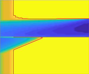
The eigenfunction again supports the classification, this time as a CF-type mode. The eigenfunction for the most unstable mode at the point $\varGamma =0.4$, $\varOmega =0.4875$ (with ${ {Re}}=500\,000$) is shown in figure 11(a), and displays an oscillatory structure with decay beyond the vertical line (which indicates the WKB turning point), similar to the mode shown in figure 6(b). Although this time the localisation at the left boundary is much stronger, the mode is observed to share more similarities with the CF mode of figure 6 than the Tollmien–Schlichting mode shown in the same figure. In figure 11(b), as a further example for the orange region closer to $\varGamma =1$, the eigenfunction is shown for a 3-D mode instability at the point $\varGamma =0.975$, $\varOmega =0.49375$, which again has similarities with the CF mode already presented above, and this time the localisation is weaker.

Figure 11. Same as figure 6, but with parameters (a) $\varGamma =0.4$, $\varOmega =0.4875$, ${ {Re}}=500\,000$, $k_x=5$ and $k_z=63$, and (b) $\varGamma =0.975$, $\varOmega =0.49375$, ${ {Re}}=5000$, $k_x=0.3$ and $k_z=6$. This figure shows that the eigenfunction structure of the 3-D mode instability investigated in figure 10 has similarities with that of figure 6(b), further suggesting it is of CF type. It also demonstrates this for a further example of an identified 3-D mode instability.

The eigenfunctions are a quick way to classify whether the 3-D mode is a modified Tollmien–Schlichting or CF type. The modified Tollmien–Schlichting instability is expected to exist only close to $\varGamma =0.15$, and so it is likely that the 3-D mode regions for larger $\varGamma$ values are due to the finite Reynolds number effects and the CF instability. Both types of 3-D mode instabilities seem to prefer anticyclonic rotation, and so are not observed towards the bottom of the unstable region.

The instability branches seen in figure 8(f) and figure 10(a) are very small in wavenumber space, suggesting a more fine wavenumber resolution is required to fully capture these instabilities. This is the reason that the 3-D mode regions (orange in figure 4) appear to exist in a quite patchy and random manner. Here we have had to sacrifice the resolution in wavenumber to be able to investigate a broad range of other parameters.

3.3. Semi-localised eigenfunctions

An interesting trend in the numerical data (used to plot figure 3) is that as the parameters are changed and moved towards the edge of the CF instability region (e.g. $\varOmega$ is moved towards $0.5$ from below), the $k_z$ wavenumber of the destabilising mode increases alongside the critical Reynolds number. The latter indicates that the instability can be captured by an inviscid approximation in which the governing eigenvalue problem given by (2.7)–(2.12) reduces to a simple second-order ordinary differential equation (ODE) for $\hat {v}$ (recall ${ {Pr}}=\infty$, $N=0$ and $\hat {\rho }=0$, so (2.11) is not needed):

(3.1)\begin{equation} \hat{v}''+k_z^2b(y)\hat{v}=0, \quad b(y)={-}\left[1+\frac{2\varOmega}{\sigma^2}(2\varOmega-U_B')\right] \end{equation}

(see Billant & Gallaire (Reference Billant and Gallaire2005) for an equivalent cylindrical base flow expression). The fact that $k_z \gg 1$ means that a WKB (short-wavelength) approximation can also be used. The numerical results show that the frequency is consistently many orders of magnitude smaller than the growth rate, so that $\sigma _i \ll \sigma _r$, and we will use $\sigma \simeq \sigma _r$ in the following. The nature of the solution is determined by the sign of the function $b(y)$: positive and the solution is oscillatory in space, negative and the solution is exponentially growing/decaying. Because of this, a location of $y$ where $b(y)=0$ (a WKB turning point $y_t$) causes a change in behaviour of the solution. When there is only one turning point in the domain, which is the case here as $U_B'$ is only linear in $y$ so

(3.2)\begin{equation} y_t = \frac{1}{2(1-\varGamma)}\left[ 1-2\varOmega-\frac{\sigma^2}{2\varOmega} \right], \end{equation}

the oscillatory or wave-like part of the solution can be trapped on one of the channel walls, and is referred to as being ‘semi-localised’. In order to have fully localised unstable modes, two turning points are needed within the domain, with oscillatory behaviour between them and decay towards each wall. A cubic base flow is sufficient to force the two turning points, as then $U_B'$ is quadratic in $y$. Appendix C demonstrates that localised CF modes exist for a cubic base flow that remains close to a simple PCF.

For the CPF problem, further CF eigenfunctions are plotted in figure 12 at $\varGamma =0.1$ and $\varOmega =0.25,0.45$, with a dotted grey line showing the turning point. There is a good match with the localisation observed in both eigenfunctions. It can be seen directly from (3.2) that for fixed $\varGamma =0.1$, stronger localisation is found for larger $\varOmega$. For larger $\varGamma$ values, taking $\varOmega$ too small results in $y_t>1$ and no localisation is observed. The turning point location in (3.2) estimates the localisation of the eigenfunctions very well even for the CF modes of figures 6 and 11, where $k_z$ is not so large. WKB solutions can also be found for $k_x >0$ but then the turning points are in the complex plane and the analysis more delicate (Billant & Gallaire Reference Billant and Gallaire2005). Analytical solutions are also available in the streamwise-independent, inviscid and linear CPF problem as a linear combination of Airy functions, but this is not pursued here.

Figure 12. Same as figure 6, but with parameters (a) $\varGamma =0.1$, $\varOmega =0.25$, ${ {Re}}=1000$, $k_x=0$ and $k_z=7.8$, and (b) $\varGamma =0.1$, $\varOmega =0.45$, ${ {Re}}=60\,000$, $k_x=0$, $k_z=46$. The displayed eigenfunctions demonstrate how the trapping length scale of the mode between a WKB turning point and the wall is highly dependent on the parameters.

All the eigenfunctions shown are localised on the left wall, and this can be directly observed from the WKB governing equation. In fact, rewriting the function $b(y)$ using $y_t$ gives

(3.3)\begin{equation} b(y) ={-}(y-y_t)\frac{4\varOmega}{\sigma^2}(1-\varGamma). \end{equation}

For the localisation of an unstable mode to occur on the left-hand (right-hand) side of the channel, the sign of $b(y)$ would have to be positive for $y< y_t$ ($y>y_t$). Observe then that localisation occurs on the left-hand side of the channel for anticyclonic rotation ($\varOmega >0$), whereas localisation occurs on the right-hand side of the channel for cyclonic rotation ($\varOmega <0$). Semi-localised CF eigenfunctions (i.e. those that are trapped on one side of the domain, decaying towards the opposite wall) have already been identified in the literature (e.g. Leclercq et al. Reference Leclercq, Nguyen and Kerswell2016; Park et al. Reference Park, Billant and Baik2017, Reference Park, Billant, Baik and Seo2018).

4.1. Anticyclonic rotation ($\varOmega >0$)

To probe the instability types found for anticyclonic rotation, and the relative strength of the instabilities, growth rate spectrums over wavenumber space are presented. Figure 14 shows six different plots, which vary the rotation rate from $0$ to $1$ for PPF ($\varGamma =0$). Four branches of instability are seen in the non-rotating flow, in good agreement with the results shown in figure 4.12 of Chen (Reference Chen2016) and figure 6 of Le Gal et al. (Reference Le Gal, Harlander, Borcia, Le Dizès, Chen and Favier2021), corresponding to the non-rotating flow ($\varOmega =0$). They identify the branch extending from $k_z=0$ as a Tollmien–Schlichting instability, whereas the other branches correspond to resonance instabilities between Tollmien–Schlichting modes and IGWs. The Tollmien–Schlichting instability branch remains as $\varOmega$ increases, but reduces in size as $\varOmega$ approaches $1$. This branch requires no further study in the presence of stratification. The stratification plays no part in the eigenvalue problem for the $k_z=0$ modes, and introducing a non-zero $k_z$ does not qualitatively change the eigenfunctions. A large unstable branch appears for rotating PPF, attached to $k_x=0$ for smaller rotation rates, and it is much more unstable than the Tollmien–Schlichting instability, although it stabilises again as $\varOmega$ approaches $1$.

Figure 14. A sequence of growth rate plots over wavenumber space. The rotation rate increases going from (a) to (f). For this sequence, the flow is PPF ($\varGamma =0$), $N=2$ and ${ {Re}}=50\,000$. White space is plotted where the wavenumber pairs are stable. This figure demonstrates how the large instability branch is stabilised with increasing $\varOmega$, but the small thin branch connected to $k_z=0$ (identified as a Tollmien–Schlichting instability) is present for all rotation rates.

This large branch is expected to be a stratification-modified CF instability, due to the connection with the unstable $k_x=0$ modes and its stabilisation for larger $\varOmega$ values. To investigate and confirm its origin, it is useful to look at its transition as non-zero $N$ is introduced and increased towards $2$. This is presented for $\varOmega =0.2$ in figure 15. In the unstratified flow, we see two types of instability from the previous section: Tollmien–Schlichting and CF. The CF branch dominates wavenumber space and has larger growth rates. As $N$ is increased, the branch shrinks, with more wavenumber pairs stabilised by increasing $N$, but clearly the large unstable branch in figure 14 has evolved from the CF branch, and is classified as a stratification-modified CF instability. The evolution of this branch displays the feature that for strong enough $N$, the most unstable mode moves from away $k_x=0$.

Figure 15. A sequence of growth rate plots over wavenumber space. The buoyancy frequency $N$ increases going from (a) to (f). For this sequence, the flow is PPF (i.e. $\varGamma =0$), $\varOmega =0.2$ and ${ {Re}}=50\,000$. White space is plotted where the wavenumber pairs are stable. This figure aids in classifying the large instability branch found in figure 14 as a stratification-modified CF instability, by showing a transition of the instability branches in wavenumber space as stratification is introduced and gradually increased (as the instability types are known for the unstratified flow).

The transition from $\varOmega =0.4$ to $\varOmega =0.6$ in figure 14 crosses the critical $\varOmega$ where Rayleigh's criterion states that the flow should become stable to streamwise-independent perturbations (even for stratified flow, see Appendix B), and this is observed as the branch moves away from the axis.

Figure 16 shows the eigenfunctions for the most unstable wavenumber pairs of the $\varOmega =0.2,0.4$ and $0.6$ plots in figure 14. The branch for $\varOmega =0.2$ was identified to be a CF-type instability, and the eigenfunction in figure 16(a) clearly supports that when comparing it to a characteristic CF-type eigenfunction in the unstratified flow, for example figure 12(a) (or when comparing with CF modes identified in the literature, e.g. Park et al. Reference Park, Billant and Baik2017, Reference Park, Billant, Baik and Seo2018). The short transition first to $\varOmega =0.4$ and then to $\varOmega =0.6$ shows that, although the qualitative structure is somewhat different for $\varOmega =0.6$, it is, in fact, the same type of mode. We also still see the localisation on one side of the domain. This is expected for stratified CF instability with $k_x=0$, as the analysis of § 3.3 can be easily modified to include the effects of stratification Billant & Gallaire (Reference Billant and Gallaire2005). Despite non-zero $k_x$ here, we still observe the localisation, which supports the argument that these branches of instability in the plots of figure 14 can be classified as CF-type instabilities. Finally, the discussion in Appendix D further supports the classification of these modes as CF-type instabilities, as we do not see interactions between frequency branches, or thin ranges of instability in $k_z$. A CF-type instability modified by stratification is therefore observed beyond the Rayleigh line. Interestingly, this instability cannot be captured by a WKB analysis with $k_x>0$ as stratification is only found to play a secondary role there (Billant & Gallaire Reference Billant and Gallaire2005). This indicates that there is no $k_z \rightarrow \infty$ limit for these stratification-modified CF instabilities.

Figure 16. Eigenfunctions of the most unstable mode for parameter values $\varGamma =0$, $N=2$, ${ {Re}}=50\,000$, along with (a) $\varOmega =0.2$, $k_x=2.4$ and $k_z=59.6$, (b) $\varOmega =0.4$, $k_x=4$ and $k_z=45.9$ and (c) $\varOmega =0.6$, $k_x=3.2$ and $k_z=30$. The blue and red lines are the $\hat {u}$ and $\hat {v}$ components of the velocity perturbation, with solid and dashed lines showing the real and imaginary parts. The plots are only shown up to $y=0.6$ as the eigenfunctions decay to zero. This figure shows, first, that for smaller $\varOmega$ the qualitative shape of the eigenfunctions is similar to the CF modes in the unstratified flow (e.g. figure 12a) and, second, that the gradual change in shape allows the same classification to be made for the instabilities at larger $\varOmega$ values.

The ‘ripple’-type feature near the CF branch in the $\varOmega =0.2$ plot of figure 14 looks like a candidate for a resonance instability, as the literature shows that the resonance mechanism leads to small unstable $k_z$ ranges for a chosen $k_x$ (Vanneste & Yavneh Reference Vanneste and Yavneh2007; Wang & Balmforth Reference Wang and Balmforth2018). This can be confirmed further by investigating the coincidence of frequency branch crossings with positive growth rates, and is done in Appendix D. This analysis also reveals that as $k_z$ increases, a different mechanism takes over, with the properties suggesting a CF instability. It is not surprising that a resonance instability has overlap with the CF-type instability, as they can be difficult to distinguish (Leclercq et al. Reference Leclercq, Nguyen and Kerswell2016). Although Park et al. (Reference Park, Billant and Baik2017, Reference Park, Billant, Baik and Seo2018) study TCF, their studies of the competition between CF instability and SRI reveal that one of the main distinguishing features is that the streamwise-dependent CF instability modes are only weakly dependent on the streamwise spatial variable when compared with SRI (meaning they have smaller azimuthal or horizontal wavenumber). This is in good agreement with the classifications we have made here, as the ripples are observed on the larger $k_x$ side of the modes that have been identified to be CF type. The growth rates are dominated by the CF-type instability and the ripple effect is only seen where the CF-type instability is weak.

Figure 17(a) displays the eigenfunction of a mode in the lowest ripple of the instability in the $\varOmega =0.2$ plot of figure 14, and figure 17(b) displays a mode in the fourth ripple from the bottom. The eigenfunction shapes are not similar to those reported above, apart from there does appear to be some localisation towards the left boundary, despite it being fairly weak. The number of oscillations within the region trapped on the left boundary increases as we move up the ripple-type branches, characteristic of resonance instabilities (Le Dizès & Riedinger Reference Le Dizès and Riedinger2010; Park et al. Reference Park, Billant and Baik2017; Wang & Balmforth Reference Wang and Balmforth2018). There are some instabilities related to SRI that are found to be localised at one boundary, such as the RI (Billant & Le Dizès Reference Billant and Le Dizès2009; Le Dizès & Billant Reference Le Dizès and Billant2009; Le Dizès & Riedinger Reference Le Dizès and Riedinger2010; Riedinger et al. Reference Riedinger, Le Dizès and Meunier2011), or due to the presence of baroclinic critical layers (Wang & Balmforth Reference Wang and Balmforth2018), but these mechanisms cause the instability in wavenumber space to become continuous again, which would then not appear as ripples. It is difficult to classify this instability precisely based on the eigenfunctions, but it is likely that it is related to a resonance instability due to the factors discussed previously. Regardless of their origin, the branches are dominated by the CF-type instability in terms of growth rates, and so this is not a region of parameter space where resonance instabilities will dominate.

Figure 17. Same as figure 16, but with parameters $\varGamma =0$, $\varOmega =0.2$, $N=2$ and ${ {Re}}=50\,000$, along with (a) $k_x=8.3$ and $k_z=29.5$, and (b) $k_x=9.4$ and $k_z=42.2$. The figure shows that the eigenfunctions of instabilities present in the ripples of figure 14 do not provide an easy classification of the type of mode, although the number of oscillations appears to correspond to the different ripples.

Figure 18 presents a similar analysis of varying rotation rate to figure 14, but now for PCF ($\varGamma =1$). This is done at ${ {Re}}=5000$ as PCF is more unstable than PPF for arbitrary rotation rate. The non-rotating flow displays only one branch of instability, which was identified by Facchini et al. (Reference Facchini, Favier, Le Gal, Wang and Le Bars2018) as a resonance of IGWs. A non-zero anticyclonic rotation brings with it strong instabilities which persist at all of the tested rotation rates, although it is weaker for larger $\varOmega$ values. These plots are similar to those for PPF presented in figure 14, and so much of the discussion remains valid, although there are some clear differences in that shape of the branch for larger $\varOmega$, as well as the size of the ripple effect.

Figure 18. Same as figure 14, but now the flow is PCF ($\varGamma =1$), $N=2$ and ${ {Re}}=5000$. The figure again shows various branches of instability, with the larger branches being stabilised as $\varOmega$ is increased, although they do persist all the way to $\varOmega =1$.

A gradual increase of the stratification from an unstratified fluid to $N=2$, in the same way as was done for PPF in figure 15, suggests that the large branch in the $\varOmega =0.2$ plot of figure 18 should be classified as a stratification-modified CF instability. Focusing on the eigenfunctions and gradually changing $\varOmega$ suggests this classification carries through to larger $\varOmega$ values. Once again, we observe that instability persists beyond the Rayleigh line, and it can be classified as a CF-type modified by stratification.

Beyond $\varOmega =0.5$, which is the Rayleigh line for PCF, valid for streamwise-independent $k_x=0$ perturbations in an inviscid fluid, the flow appears to still be unstable towards the $k_z$-axis. The growth rates in fact decay towards the axis and the flow is stable on it, meaning it satisfies Rayleigh's criterion here and, in fact, the finite ${ {Re}}$ value causes the instability region to spread closer to that axis.

The ripple effect appears again, but this time with thicker branches, although there are fewer of them. Eigenfunctions of the unstable modes on these branches are presented in figure 19, with figure 19(a) displaying that of a mode in the lowest ripple of the instability in the $\varOmega =0.2$ plot of figure 18, and figure 19(b) displaying a mode in the next ripple up. Both eigenfunctions resemble the resonance-type SRI modes in the inviscid WKB literature to some extent (Wang & Balmforth Reference Wang and Balmforth2018), with localisation at each boundary, but this localisation is not clear and could be obscured by viscosity. This is most clearly observed through the variable $\hat {v}$ in figure 19(a), with real part showing the component localised at the left boundary and imaginary part showing the localisation at the right boundary. The second of these plots has more oscillations in the region on the left, which is expected as we move up through the ripples. This displays the characteristic features of a resonance-type SRI, although it remains dominated by the stratification modified CF instability.

Figure 19. Same as figure 16, but with parameters $\varGamma =1$, $\varOmega =0.2$, $N=2$ and ${ {Re}}=5000$, along with (a) $k_x=3$ and $k_z=7.5$ and (b) $k_x=3$ and $k_z=13$. The shown eigenfunctions demonstrate possible resonance between two modes trapped at either side of the domain, although the decay towards the opposite wall is not strong. The number of oscillations again corresponds to different ripples in figure 18.

By gradually increasing the rotation rate from $\varOmega =0$ to $\varOmega =0.2$ (not shown here), we can observe that the IGW–IGW resonance instability branch found for $\varOmega =0$, first identified by Facchini et al. (Reference Facchini, Favier, Le Gal, Wang and Le Bars2018), is smoothly connected to the large unstable branch found for $\varOmega =0.2$. This branch grows with increasing $\varOmega$, and merges with another branch that extends out from $k_x=0$, to produce what is seen for $\varOmega =0.2$ in figure 18. The same gradual change can be used to track the eigenfunctions, showing how the resonance of two modes localised at each side of the channel gradually changes and becomes more of a global mode with the increase of $\varOmega$. This process highlights again the difficulties in distinguishing the origins of the instability branches. However, the largest ripple that extends out from the main branch is clearly seen to develop from the IGW–IGW resonance, supporting the classifications made earlier.

The Reynolds number chosen for $\varGamma =0$ was 10 times larger than that chosen for $\varGamma =1$, as the flow appears to stabilise with decreasing $\varGamma$. Because of this, it is difficult to isolate the effects of changing $\varGamma$. To probe the $\varGamma$ dependence, we consider both changing $\varGamma$ and changing ${ {Re}}$ values, noting that we cannot focus on the size of the instability region (as this will be heavily influenced by ${ {Re}}$), but only on the shape of the instability branch and the types of modes that are unstable.

Figure 20 again shows sequences of growth rate plots, but now for each sequence, the values of $N$ and $\varOmega$ are fixed, and we vary both $\varGamma$ and ${ {Re}}$. The choices of $\varOmega$ values correspond to two cases: one where we expect $k_x=0$ CF instability, and one where we do not.

Figure 20. Growth rate contours for $N=2$, with $\varOmega =0.2$ (a–e) or $\varOmega =0.6$ (f–j). Here $\varGamma$ and ${ {Re}}$ are varied as shown in the plot. Each colour bar is valid for the full row of plots, and it has smaller values for (f–j) due to the flow being more stable for the larger $\varOmega$ value. The figure demonstrates how the shape of the instability branches is dependent on $\varGamma$, although most of the qualitative changes happen for $\varGamma >1/2$.

For both sequences (i.e. both rotation rates), apart from the stabilisation of the Tollmien–Schlichting modes once $\varGamma =0.25$ is reached, the qualitative picture of the unstable region is unaltered as $\varGamma$ is increased from zero to $\varGamma =0.5$, so we do not expect a change in the instabilities that are supported by the flow. Increasing $\varGamma$ further, from $\varGamma =0.5$ through $\varGamma =0.75$ and to $\varGamma =1$, we observe changes in each sequence. For the first, shown in the top line of the figure with $\varOmega =0.2$, although the main bulk of the unstable region is largely unchanged, we observe that the number of ripple features attached to the right-hand side of the unstable region is reduced. According to our earlier classification, this suggests the number of unique resonances that are unstable is reducing as we move towards PCF (although this number will be influenced by ${ {Re}}$). For the second sequence, shown in the bottom row of the figure with $\varOmega =0.6$, we see a significant change in the shape of the unstable region, becoming more elongated and reaching to larger $k_x$ values. The thin extension part of this region (i.e. the largest $k_x$ values) resembles a single ripple (e.g. in figure 20e), which could suggest the appearance of a resonance instability, according to our earlier classifications. However, it is important to note that apart from the very largest unstable $k_x$ values, this unstable region has fairly significant thickness in $k_z$ which we would not associate with a resonance, making it difficult to classify (see Appendix D). Eigenfunctions also support the conclusion that no qualitative changes occur between $\varGamma =0$ and $\varGamma =0.5$, being almost identical in that range of $\varGamma$ to figure 16(a and c).

With these observations, we chose $\varGamma =0.75$ for a more detailed study of a mixed profile. The growth rate spectrum plots are found to be qualitatively similar to those presented in figure 18 for PCF (with some slight variation in the shape), and so they are not presented here. The variation in $\varGamma$ needed to capture all the behaviours can then be reduced to a smaller range by making use of our previous observations.

4.2. Cyclonic rotation ($\varOmega <0$)

Cyclonic rotation is indistinguishable from anticyclonic rotation in the case of the stability of PPF, due to the symmetry of the flow about the channel's midpoint. However, this symmetry is broken for $\varGamma >0$ and cyclonic flow is found to be much more stable for both $\varGamma =0.75$ and $\varGamma =1$. Up to the largest ${ {Re}}$ tested ($10^6$), the cyclonic flows for both $\varGamma$ values were stable for $\varOmega \leq -0.4$. Figure 21 displays contour plots of the growth rates over wavenumber space for both $\varGamma$ values, calculated at the maximum ${ {Re}}$ value of ${ {Re}}=10^6$, for $\varOmega =-0.2$. The thin strips suggest resonances play a part in the instability.

Figure 21. Growth rates over wavenumber space for two different values of $\varGamma$. The constant parameter values here are $\varOmega =-0.2$, $N=2$ and ${ {Re}}=10^6$.

Eigenfunctions, shown in figure 22, support the classification of this instability as resonance-type SRI, as they are a combination of two structures each localised at sides of the domain. The eigenfunctions shown in figure 22(a,c) are on the most unstable branch of $\varGamma =0.75$ and $\varGamma =1$, respectively, whereas the middle eigenfunction is on the branch that sits slightly higher and to the right of the most unstable one for $\varGamma =0.75$, which is why there is more oscillatory behaviour (similar to the observations about figure 19). For cyclonic flow, KWs cannot be part of a resonant pair so resonance-type SRI must be between IGWs, and the more oscillatory branch corresponds to a higher-order IGW (Wang & Balmforth Reference Wang and Balmforth2018).

Figure 22. Eigenfunctions of the most unstable mode for parameter values $\varOmega =-0.2$, $N=2$ and ${ {Re}}=10^6$, along with (a) $\varGamma =0.75$, $k_x=4.4$ and $k_z=12$, (b) $\varGamma =0.75$, $k_x=4.7$ and $k_z=15.9$, and (c) $\varGamma =1$, $k_x=3.6$ and $k_z=9.65$. The blue lines are the $\hat {u}$ component of the velocity perturbation and the red lines are the $\hat {v}$ component, with solid lines showing the real part and dashed lines showing the imaginary part. The eigenfunction shapes aid in the classification of these modes as resonance-type instabilities, as they appear to be two waves localised at the boundaries, with some interaction in the middle region (although the decay towards the opposite boundary is still not strong).

Although the introduction of stratification acts to move CF instability above the Rayleigh line at $\varOmega =0.5$, it does not appear to move the instability below the Rayleigh region and into the cyclonic regime, meaning stratification modified CF instability is not supported by cyclonic rotation. Comparing anticyclonic and cyclonic rotation of the same magnitude, i.e. comparing the $\varOmega =0.2$ plot of figure 18 with the $\varGamma =1$ plot of figure 21, we observe that not only do we need a much larger Reynolds number in order to see instability for cyclonic rotation, but we also find that the growth rates are much smaller. The key conclusion here then is that cyclonic rotation is the only regime where resonance instabilities have the largest growth rates: resonance instabilities are swamped by stratification-modified CF instability for anticyclonic flow.

4.3. The effects of strong stratification and thermal diffusion

To investigate the flow with stronger stratification, $N=10$ was chosen. For all three $\varGamma$ values, the plots showing varying anticyclonic rotation rate are qualitatively similar to those for $N=2$, with only a few key differences, and so they are not presented here. First, for PPF, it appears that the Tollmien–Schlichting mode instability branch is not affected by this significant increase in the strength of stratification, and plotting the growth rates in wavenumber space at the same ${ {Re}}$ as before ($50\,000$), reveals that the other instabilities are stabilised and the Tollmien–Schlichting instability is all that remains, meaning it becomes the strongest instability at larger $N$ values. For both $\varGamma =0.75$ and $\varGamma =1$, stabilisation due to increased stratification is also observed, and in order to see any instability, a search at higher Reynolds number must be done. Plotting with $10\times$ the Reynolds number as those for $N=2$ produces qualitatively similar plots. This was expected; although stratification can destabilise the flow, it is also expected that stronger stratification may restabilise the flow (Dubrulle et al. Reference Dubrulle, Marié, Normand, Richard, Hersant and Zahn2005).

The plots showing growth rates over wavenumber space for stronger stratification ($N=10$) and cyclonic rotation with strength $\varOmega =-0.2$, are shown in figure 23. These plots show some clear differences with figure 21: the branches have slightly different shapes and reach much higher values for both wavenumbers. There are also significantly more branches of instability appearing here. This might have been expected by comparing with a study by Park & Billant (Reference Park and Billant2013), of resonance instabilities in TCF. They find that when the outer cylinder is rotating faster than the inner (which would correspond to a cyclonic flow), the resonance instabilities require strong stratification, and thus as stratification becomes stronger, more of this instability is introduced. Eigenfunctions are not shown again here, but they do show localisation on the two sides of the domain, with a branch that is higher corresponding to more oscillatory behaviour in space, as expected for resonance-type SRI.

Figure 23. Same as figure 21, but $N=10$. The figure suggests that even for stronger stratification, the resonance instabilities are the only ones present in the flow.

Thermal diffusion effects can be added through a finite ${ {Pr}}$ value, with ${ {Pr}}=7$ chosen here to align with experimental studies of heated fluids (e.g. Gellert & Rüdiger Reference Gellert and Rüdiger2009; Seelig, Harlander & Gellert Reference Seelig, Harlander and Gellert2018; Lopez et al. Reference Lopez, Lopez and Marques2023). The introduction of thermal diffusion only appears to stabilise the flow, reducing the growth rates and the size of the unstable region wavenumbers. The change from ${ {Pr}}=\infty$ to ${ {Pr}}=7$ is not significant, and instability is still observed in the majority of cases at the same Reynolds number. This was again expected, as Dubrulle et al. (Reference Dubrulle, Marié, Normand, Richard, Hersant and Zahn2005) state that thermal diffusion has a stabilising effect, in their study of stratified and rotating PCF. Stronger diffusion through smaller ${ {Pr}}$ values could have a more significant effect, but we do not explore that regime here.