


1. Introduction
Electrospray is well known for its ability to produce charged droplets and thin fibres from liquids. Electrosprays can operate in a variety of regimes depending on the physical properties of the liquid, its flow rate and the potential difference applied to the emitter (Cloupeau & Prunet-Foch Reference Cloupeau and Prunet-Foch1989). The cone-jet regime has been thoroughly studied because it atomizes liquids into droplets with narrow size distributions and controllable average diameters down to a few nanometres (Cloupeau & Prunet-Foch Reference Cloupeau and Prunet-Foch1990; Gañán-Calvo & Montanero Reference Gañán-Calvo and Montanero2009; Gamero-Castaño Reference Gamero-Castaño2010; Herrada et al. Reference Herrada, López-Herrera, Gañán-Calvo, Vega, Montanero and Popinet2012; Gamero-Castaño Reference Gamero-Castaño2019). The meniscus of a cone-jet resembles the ideal Taylor cone (Taylor Reference Taylor1964), except for the formation of a jet emanating from its vertex and whose natural breakup leads to the formation of charged droplets. The electric field on the meniscus exhibits a maximum in the cone-to-jet transition (Gamero-Castaño & Fernández De La Mora Reference Gamero-Castaño and Fernández De La Mora2000). This maximum is a function of the physical properties of the liquid, namely the surface tension, density, dielectric constant and most importantly the electrical conductivity. Liquids with electrical conductivities near  $1\ {\rm S}\ {\rm m}^{-1}$ produce jets and droplets with diameters of a few tens of nanometres, and electric fields exceeding $1\ {\rm V}\ {\rm nm}^{-1}$. Ions can be emitted from surfaces sustaining such electrification levels in a process referred to as ion field emission. In the case of cone-jets, ion field emission can take place from droplets and from the vertex of the cone (Gamero-Castaño & Fernández De La Mora Reference Gamero-Castaño and Fernández De La Mora2000). Emission from the vertex leads to the ion emission regime, i.e. to the liquid being fully electrosprayed into molecular ions without the formation of charged droplets. The ion emission regime has technological applications in electric propulsion for spacecraft (Romero-Sanz, de Carcer & de la Mora Reference Romero-Sanz, de Carcer and de la Mora2005; Lenguito et al. Reference Lenguito, Fernandez Garcia, Fernandez de la Mora and Gomez2010; Lenguito, de la Mora & Gomez Reference Lenguito, de la Mora and Gomez2011; de la Mora Reference de la Mora2010; Hsu et al. Reference Hsu, Brady, Easton, Labatete-Goeppinger, Curtiss, Krejci and Lozano2019; Kristinsson et al. Reference Kristinsson, Freeman, Petro, Lozano, Hsu, Young and Martel2019; Jia-Richards, Corrado & Lozano Reference Jia-Richards, Corrado and Lozano2022; Pettersson, Jia-Richards & Lozano Reference Pettersson, Jia-Richards and Lozano2022) and compact ion sources (Zorzos & Lozano Reference Zorzos and Lozano2008; Zorzos Reference Zorzos2009; Fedkiw & Lozano Reference Fedkiw and Lozano2009; Perez-Martinez et al. Reference Perez-Martinez, Guilet, Gierak and Lozano2011; Guilet et al. Reference Guilet, Perez-Martinez, Jegou, Lozano and Gierak2011; Xu, Tao & Lozano Reference Xu, Tao and Lozano2018). Ion field emission is modelled as a kinetic process in which the ion, in order to evaporate from the surface, must overcome an energy barrier that depends on the ion–liquid pair, i.e. on the ion solvation energy, and which is lowered by the electric field. Müller (Reference Müller1941, Reference Müller1956) and Iribarne & Thomson (Reference Iribarne and Thomson1976) developed expressions for the energy barrier based on the image charge induced by the ion as it moves away from the surface of the liquid.
Cone-jets are typically operated from capillary tubes, a configuration that enables feeding a liquid in a wide range of flow rates by simply imposing a pressure difference. Although the ion emission regime can also be implemented in capillary tubes (Garoz et al. Reference Garoz, Bueno, Larriba, Castro, Romero-Sanz, Fernández de La Mora, Yoshida and Saito2007), it is more often realized in externally wetted emitters (Lozano & Martinez-Sanchez Reference Lozano and Martinez-Sanchez2005b; Castro et al. Reference Castro, Larriba, Fernandez de la Mora, Lozano and Sümer2006). It is not understood why similar liquids operate in either the cone-jet or the ion emission regimes. A high electrical conductivity,  $K \gtrsim 1\ {\rm S}\ {\rm m}^{-1}$, is important for operation in the ion emission regime, which is explained by the scaling of the maximum electric field in cone-jets (Gamero-Castaño & Magnani Reference Gamero-Castaño and Magnani2019) and the electrostatic reduction of the energy barrier. However, at room temperature an ionic liquid like 1-ethyl-3-methylimidazolium tetrafluoroborate, [C $_2$C
$_2$C $_1$Im][BF $_4$], can operate in the ion emission regime, while the ionic liquid 1-ethyl-3-methylimidazolium bis((trifluoromethyl)sulfonyl)imide, [C $_2$C
$_2$C $_1$Im][Tf $_2$N], having a similar conductivity, only operates in the cone-jet mode. The solvation energy is a key parameter in ion emission, but this property has not been measured for most ion–liquid pairs and can only be estimated. Concentrated NaI/formamide solutions electrosprayed from a capillary tube transition from the cone-jet mode to a mixed droplet/ion emission regime at sufficiently low flow rate (Gamero-Castaño & Fernández De La Mora Reference Gamero-Castaño and Fernández De La Mora2000). The [C $_2$C
$_2$C $_1$Im][BF $_4$] electrosprayed from a capillary tube behaves similarly, a combination of droplets and ions are produced at most flow rates while the ion emission regime occurs at low flow rates (Chiu et al. Reference Chiu, Levandier, Austin, Dressler, Murray and Lozano2003). Ionic liquids that operate in the ion emission regime when electrosprayed from externally wetted emitters also produce charged droplets if the flow rate is sufficiently high (Ticknor, Miller & Chiu Reference Ticknor, Miller and Chiu2009).
The ion emission regime was first modelled by Higuera (Reference Higuera2008), who considered emission from an isolated droplet on a conductive surface. Coffman (Reference Coffman2016) expanded Higuera's work by adding the dynamics of a feed system that supplies liquid to the meniscus. This work also considered self-heating of the liquid. Recently, Gallud & Lozano (Reference Gallud and Lozano2022) developed a model that includes net free charge in the liquid, originated by conductivity gradients associated with self-heating and temperature variations. Gallud & Lozano analyse the stability limits of the ion emission regime, identifying two different upper stability limits related to the maximum current output and the maximum electric stress a liquid meniscus can withstand. This work also highlights the importance of dissipation, which increases the maximum electric field at which the ion emission regime is stable. Gallud & Lozano find that the increase of the temperature does not affect the ion current when the hydraulic impedance of the system is constant, a result that may be related to the linear dependence between conductivity and temperature used in this model. Furthermore, the heat dissipated is efficiently transported to the wall of the emitter, resulting in a small temperature increase near the tip, approximately  $5\,\%$. However, ionic liquids have an exponential dependence between conductivity and temperature and this (Okoturo & VanderNoot Reference Okoturo and VanderNoot2004; Leys et al. Reference Leys, Wübbenhorst, Preethy Menon, Rajesh, Thoen, Glorieux, Nockemann, Thijs, Binnemans and Longuemart2008), together with the exponential ion evaporation law, can have significant impacts on the current emitted.
This article develops a steady-state model for ion emission from a meniscus anchored on a finite, cylindrical emitter. Section 2 describes the first-principles model, and introduces a simpler analytical model with the goal of deriving the characteristic length of the emission region. Section 3 explains the numerical methods for solving the system of equations. Section 4 analyses the numerical solution using [C $_2$C
$_2$C $_1$Im][BF $_4$] as a case study, and derives the scaling law for the ion current and a criterion for the onset of the ion emission regime. This criterion depends on the physical properties of the liquid, and correlates well with experimental observations. A summary of the work is presented in § 5.
2. Model for an ion-emitting Taylor cone
2.1. Computational domain
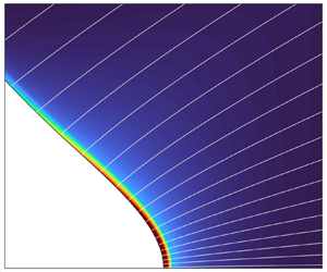
Figure 1 shows the computational domain. We use cylindrical coordinates  $\{x,r\}$. The emitter is modelled as an equipotential cylinder with surfaces $\varSigma _{1e}$ and $\varSigma _{2e}$, supporting a Taylor cone with a free surface $\varSigma _{12}\cup \varSigma _{34}$. Here $R(x)$ is the radius of the cross-section of the cone. The domain is enclosed by an outer boundary formed by a plane $\varSigma _{1c}$ perpendicular to the emitter, and the surface $\varSigma _{1o}$ placed far enough from the meniscus so that the particular choice of position does not significantly affect the solution. The bulk of the Taylor cone is divided into regions 2 and 3: the ion emission regime is characterized by very small flow rates and the fluid motion and dissipation effects are expected to be significant only near the tip of the meniscus, region 3. Similarly, the space surrounding the Taylor cone is divided into regions 1 and 4 to take advantage of the sharp decrease of the space charge of the beam away from the emission area (the space charge density is only retained in region 4). The use of these regions reduces the computational time because regions 1 and 2 can be resolved with simplified equations and computational grids with lower resolution than in regions 3 and 4. The model equations are highly nonlinear and must be solved iteratively. The extent of regions 3 and 4 is determined in each iteration by monitoring the ion emission area and the volumetric charge density in the beam.

Figure 1. Sketch of the model domain.
2.2. Governing equations
The model is based on the leaky-dielectric formulation (Melcher & Taylor Reference Melcher and Taylor1969; Saville Reference Saville1997), extended to include ion-field emission, dissipation and the ion beam. The velocity  $\boldsymbol {V}$ and pressure $P$ fields in the liquid fulfil the continuity and conservation of momentum equations,
 \begin{gather} \boldsymbol{\nabla}\boldsymbol{\cdot}\boldsymbol{V}=0, \end{gather}
 \begin{gather} \rho\boldsymbol{V}\boldsymbol{\cdot}\boldsymbol{\nabla}\boldsymbol{V}={-}\boldsymbol{\nabla} P+\boldsymbol{\nabla}\boldsymbol{\cdot}\boldsymbol{\tau}_\mu, \end{gather}
where  $\rho$ and $\mu$ are the density and viscosity of the liquid and $\boldsymbol {\tau }_\mu$ is the viscous stress tensor,
 \begin{equation} \boldsymbol{\tau}_\mu=\mu\left(\boldsymbol{\nabla}\boldsymbol{V}+{\boldsymbol{\nabla}\boldsymbol{V}}^{\rm T}\right). \end{equation}
Ohmic and viscous dissipation are expected to be important, and the equation of conservation of energy is used to compute the associated variation in temperature  $T$,
$T$,
 \begin{equation} \rho c\boldsymbol{V}\boldsymbol{\cdot}\boldsymbol{\nabla} T=k\nabla^2T+\boldsymbol{\tau}_\mu\boldsymbol{:}\boldsymbol{\nabla}\boldsymbol{V}+\boldsymbol{E}^i\boldsymbol{\cdot}\boldsymbol{J}^i, \end{equation}
where  $c$ and $k$ are the heat capacity and thermal conductivity of the liquid, while $\boldsymbol {E}$ and $\boldsymbol {J}$ stand for the electric field and the current density. When needed, superscripts $i$ and $o$ denote inside and outside the Taylor cone, respectively. The electrical conductivity $K$ and the viscosity are strong functions of temperature, and these dependencies are modelled with exponential relations valid for ionic liquids (Okoturo & VanderNoot Reference Okoturo and VanderNoot2004; Leys et al. Reference Leys, Wübbenhorst, Preethy Menon, Rajesh, Thoen, Glorieux, Nockemann, Thijs, Binnemans and Longuemart2008),
 \begin{gather} K(T)=Y_K{\rm e}^{{B_K}/({T-T_K})}, \end{gather}
 \begin{gather} \mu(T)=Y_\mu {\rm e}^{{B_\mu}/({T-T_\mu})}, \end{gather}
where the constants  $Y_K$, $B_K$, $T_K$, $Y_\mu$, $B_\mu$ and $T_\mu$ are liquid specific. All other liquid properties are regarded constant, independent of temperature. Following the leaky-dielectric formulation, the volumetric charge density inside the liquid is assumed to be negligible and Ohm's law is used to express the current density, $\boldsymbol {J}^i = K\boldsymbol {E}^i$. Conservation of charge and the irrotational nature of the electric field then provide an equation for the electric potential $\varPhi ^i$ inside the liquid
 \begin{equation} \boldsymbol{\nabla} \boldsymbol{\cdot} (K\boldsymbol{E}^i) = 0\quad {\rm and} \quad \boldsymbol{E} ={-}\boldsymbol{\nabla} \varPhi \quad \rightarrow \quad K\nabla^2\varPhi^i+\boldsymbol{\nabla}\varPhi^i\boldsymbol{\nabla} K=0. \end{equation}
Due to the assumption of zero volumetric charge, the model cannot require the fulfilment of both conservation of charge and Gauss’ law for the electric field. To fulfil both principles, the model would need to consider a non-zero volumetric charge  $\rho _e$ and a current density $\boldsymbol {J}^i = K\boldsymbol {E}^i + \rho _e \boldsymbol {V}$. In this case, the Navier–Stokes equation (2.2) would also include the volumetric force $\rho _e \boldsymbol {E}^i$. We would like to point out that, similarly to Gallud & Lozano (Reference Gallud and Lozano2022), we had also solved the problem including this volumetric force by using a fictitious volumetric charge density $\rho _e = ({\varepsilon \varepsilon _0 \boldsymbol {\nabla }\varPhi ^i\boldsymbol {\nabla } K})/{K}$. The resulting solution is nearly identical to that of the present model. However, we have decided not to use this fictitious volumetric charge because there is no physical or mathematical justification for it.
In the vacuum surrounding the Taylor cone the electric potential  $\varPhi ^o$ fulfils Poisson equation,
 \begin{equation} \nabla^2\varPhi^o={-}\frac{\chi\omega}{\varepsilon_0}. \end{equation}
Here  $\chi$ is the charge-to-mass ratio of the ions, $\omega$ is the ion mass density and $\varepsilon _0$ is the permittivity of vacuum. Following the leaky-dielectric formulation, net charge is only present on the surface of the Taylor cone, and it is modelled as a surface charge density $\sigma$ fulfilling the conservation equation
 \begin{equation} \frac{{\rm d}}{{\rm d} x}\left(r\sigma\boldsymbol{V}\boldsymbol{\cdot}\boldsymbol{t}\right)= R (1+{R^{'}}^2)^{1/2} (KE_n^i-J_\omega), \end{equation}
where  $\boldsymbol {t}$ is the unit vector tangential to the surface and $J_\omega$ is the field-emitted ion current density. Here $E_n$ is the component of the electric field normal to the surface. Equation (2.9) balances the charge convected on the surface, the charge injected from the bulk, and the field-emitted charge. Additional equations that must be fulfilled at the surface $\varSigma _{12}\cup \varSigma _{34}$ include the jump of the normal components of the electric field, the balance of normal and tangential stresses, and the kinematic velocity constraint (the velocity component normal to the surface is coupled to the emitted current density),
 \begin{gather} E_n^o-\varepsilon E_n^i=\frac{\sigma}{\varepsilon_0}, \end{gather}
 \begin{gather} \boldsymbol{t}\boldsymbol{\cdot}\boldsymbol{\tau}_\mu\boldsymbol{n}=\boldsymbol{t}\boldsymbol{\cdot}\left(\boldsymbol{\tau}_M^o-\boldsymbol{\tau}_M^i\right)\boldsymbol{n}, \end{gather}
 \begin{gather} \gamma\boldsymbol{n}\boldsymbol{\cdot}\left(\boldsymbol{\nabla}\boldsymbol{\cdot}\boldsymbol{n}\boldsymbol{\mathsf{I}}\right)\boldsymbol{n}-P+\boldsymbol{n}\boldsymbol{\cdot}\boldsymbol{\tau}_\mu\boldsymbol{n}=\boldsymbol{n}\boldsymbol{\cdot}\left(\boldsymbol{\tau}_M^o-\boldsymbol{\tau}_M^i\right)\boldsymbol{n}, \end{gather}
 \begin{gather} \boldsymbol{V}\boldsymbol{\cdot}\boldsymbol{n}=\frac{J_\omega}{\chi\rho}. \end{gather}
Here  $\varepsilon$ and $\boldsymbol {n}$ are the dielectric constant of the liquid and the unit vector normal to the surface, respectively. The Maxwell stress tensor $\boldsymbol {\tau }_M$ is given by
 \begin{equation} \boldsymbol{\tau}_M=\varepsilon\varepsilon_0\boldsymbol{E}\boldsymbol{E}-\varepsilon_0\frac{\boldsymbol{E}\boldsymbol{\cdot}\boldsymbol{E}}{2}\left[\varepsilon-\rho\left(\frac{\partial\varepsilon}{\partial\rho}\right)_T\right], \end{equation}
where the term  $\rho (\partial \varepsilon /\partial \rho )_T$ is zero due to the incompressibility assumption. The emitted ions are accelerated away from the surface by the electric field. They are modelled as a continuum where the only significant force is that induced by the average electric field, i.e. we neglect ion–ion collisions. The continuity and conservation of momentum equations for the ion density and ion velocity $\boldsymbol {v}$ fields are
 \begin{gather} \boldsymbol{\nabla}\boldsymbol{\cdot}\left(\omega\boldsymbol{v}\right)=0, \end{gather}
 \begin{gather} \boldsymbol{\nabla}\boldsymbol{\cdot}\left(\omega\boldsymbol{v}\boldsymbol{v}\right)=\chi\omega\boldsymbol{E}^o. \end{gather}
Ion evaporation is modelled with the kinetic law proposed by Iribarne & Thomson (Reference Iribarne and Thomson1976). This equation relates the ion current density with the energy barrier that emitted ions must overcome
 \begin{equation} J_\omega=\frac{k_BT}{h}\sigma\exp\left(-\frac{{\Delta G}_S-G_E}{k_BT}\right), \end{equation}
where  $k_B$ and $h$ are the Boltzmann and the Planck constants, ${\Delta G}_S$ is the ion solvation energy and $G_E$ is the electrostatic contribution to the energy barrier. A common approach for determining $G_E$ consists of computing the electric field acting on the emitted ion as the superposition of the fields induced by its image charge and the surface charge (Müller Reference Müller1941, Reference Müller1956; Iribarne & Thomson Reference Iribarne and Thomson1976). In this article we use an improved formulation that takes into account the dielectric properties and the local curvature of the emitting surface (Magnani & Gamero-Castaño Reference Magnani and Gamero-Castaño2022),
 \begin{equation} G_E=\left(1-\frac{R_c}{r^{*}}\right)q R_c E_n^o+\frac{q^2(\varepsilon-1)}{8{\rm \pi}\varepsilon_0 R_c}\sum_{k=0}^\infty{\frac{1}{\varepsilon+1+\dfrac{1}{k}}\left(\frac{R_c}{r^{*}}\right)^{2k+2}}, \end{equation}
where  $R_c$ is the local average curvature of the surface, $r^*$ is the position of the energy barrier respect to the surface and $q$ is the charge of the ion, equal to the fundamental charge $e$ for singly charged ions. Here $r^*$ is obtained numerically (Magnani & Gamero-Castaño Reference Magnani and Gamero-Castaño2022).
2.3. Characteristic scales and dimensionless equations
We estimate the characteristic length  $L_c$ of the ion-emitting region with a simplified model for ion emission from an ideal Taylor cone. The electric field on the surface of the ideal Taylor cone (Taylor Reference Taylor1964) is given by
 \begin{equation} E_T(r)=\sqrt{\frac{2\gamma}{\varepsilon_0}\frac{\cos\theta_T}{r}}, \end{equation}
where  $r$ is the radial cylindrical coordinate and $\theta _T \cong 49.29^\circ$ is the cone semiangle (Taylor Reference Taylor1964). The electric field is singular at the vertex and will induce ion emission. Our simplified model uses (2.19) to approximate $E_n^o$, and combines (2.9), (2.10) and (2.17) to eliminate $E_n^i$ and $\sigma$ and obtain an explicit expression for the current density of emitted ions (we assume negligible surface velocity),
 \begin{equation} J_\omega(r)=\dfrac{E_T(r)}{\dfrac{\varepsilon}{K}+\dfrac{h}{\varepsilon_0 k_B T}\exp\left(\dfrac{{\Delta G}_S-G_E}{k_B T}\right)}. \end{equation}
This expression resembles Ohms law with two resistances in series and driven by the electric field: the resistance  $\varepsilon /K$ is associated with the injection of charge on the surface from the bulk, and $({h}/{\varepsilon _0 k_B T})\exp (({{\Delta G}_S-G_E})/{k_B T})$ is associated with the evaporation of ions from the surface. Thus, the current density exhibits two limiting behaviours depending on the dominance of each mechanism: far from the vertex the electric field is small, the energy barrier is large and ion evaporation restricts the transport
 \begin{equation} J_\omega(r\rightarrow\infty) \cong \frac{\varepsilon_0 k_B T}{h}\exp\left(-\frac{{\Delta G}_S-G_E}{k_B T}\right) E_T, \end{equation}
while near the vertex the electric field is large, the energy barrier is negligible, and the emission is restricted by the availability of charge injected from the bulk
 \begin{equation} J_\omega(r\rightarrow 0) \cong \frac{K}{\varepsilon}E_T. \end{equation}
In the first limit the surface charge is in near equipotential balance with the outer electric field,  $\sigma \cong \varepsilon _0E_T$, while in the second limit ion emission depletes the surface charge exponentially, $\sigma \cong [({k_B\varepsilon _0}/{hK})\varepsilon T\exp (-(({{\Delta G}_S-G_E})/{k_B T}))]^{-1} \varepsilon _0 E_T$. Note also that $r J_\omega (r)$ tends to zero towards the vertex, and therefore the total emitted current $({2{\rm \pi} }/{\sin \theta _T})\int _{0}^{\infty } r J_\omega (r) \,{\rm d}r$ remains finite. This result is non-trivial given the exponential dependence of the ion emission law on the electric field (2.17), and the singular behaviour of the field at the vertex. However, this analysis comes with the caveat that our approximation of the electric field, $E_T$, may be inaccurate near the vertex due to the depletion of the surface charge, and will need to be confirmed with the numerical solution of the first-principles model. Figure 2 plots (2.20) and its two limiting behaviours. The current density is largest near the axis and falls sharply soon after, clearly defining a region from which most of the emission takes place. We define the characteristic length of the ion-emitting region as the value of the radial coordinate where both limiting behaviours are equal, which can be written explicitly when using the energy barrier for a planar conductor, $G_E = \sqrt {q^3E_n^o / (4{\rm \pi} \varepsilon _0)}$ (Iribarne & Thomson Reference Iribarne and Thomson1976),
 \begin{equation} L_c=\frac{\cos\theta_T q^6 \gamma}{8{\rm \pi}^2{\varepsilon_0}^3{{\Delta G}_S}^4}\left[1-\frac{k_B T}{{\Delta G}_S} \ln\left(\frac{\varepsilon\varepsilon_0 k_B T}{h K}\right)\right]^{{-}4} = \alpha \frac{\cos\theta_T q^6 \gamma }{8{\rm \pi}^2{\varepsilon_0}^3 {{\Delta G}_S}^4}, \end{equation}
where  $({k_B T}/{{\Delta G}_S})\ln ({\varepsilon \varepsilon _0 k_B T}/{h K})\ll 1$ for typical ion emission conditions, e.g. it has a value of 0.101 for ${\Delta G}_S=1.6$ eV, $T=25\,^\circ$C, $\varepsilon =10$ and $K=1\ {\rm S}\ {\rm m}^{-1}$. The size of the ion-emitting region is a strong function of the ion solvation energy, proportional to the surface tension, and a weak function of the dielectric constant, the electrical conductivity and temperature.

Figure 2. Estimation of the ion current density emitted from a Taylor cone, (2.20), computed with  $T= 25\,^\circ {\rm C}$, $\varepsilon = 10$, ${\Delta G}_S = 1.6$ eV, $\gamma = 0.05\ {\rm N}\ {\rm m}^{-1}$ and $K= 1\ {\rm S}\ {\rm m}^{-1}$.
Table 1 shows the characteristic scales employed in the non-dimensionalization of the equations. The characteristic viscosity and conductivity are the values at the upstream temperature  $T_0$. The characteristic electric field is equal to the electric field on the surface of an ideal Taylor cone at $r=L_c$. The characteristic fluid velocity is obtained using the relation between the total emitted current and the flow rate $Q$, which in the ion emission regime are proportional,
 \begin{equation} Q=\frac{2{\rm \pi}}{\chi\rho}\int_S{J_\omega}\,{\rm d}S. \end{equation}
From this equation the characteristic flow rate is defined as
 \begin{equation} Q_c=\frac{2{\rm \pi}\varPhi_c K_c L_c}{\chi\rho}, \end{equation}
yielding the characteristic fluid velocity  $Q_c/{\rm \pi} {L_c}^2$. We list below the governing equations in dimensionless form, with dimensionless variables written without additional markings,
 \begin{gather} \boldsymbol{\nabla}\boldsymbol{\cdot}\boldsymbol{V}=0, \end{gather}
 \begin{gather} \boldsymbol{V}\boldsymbol{\cdot}\boldsymbol{\nabla}\boldsymbol{V}={-}\frac{\varPi_2}{2\cos\theta_T}\boldsymbol{\nabla} P+\frac{1}{{{Re}}}\left[\mu\nabla^2\boldsymbol{V}+\left(\boldsymbol{\nabla}\boldsymbol{V}+{\boldsymbol{\nabla}\boldsymbol{V}}^{\rm T}\right)\boldsymbol{\cdot}\boldsymbol{\nabla}\mu\right], \end{gather}
 \begin{gather} Pe\boldsymbol{V}\boldsymbol{\cdot}\boldsymbol{\nabla} T-\nabla^2T=\frac{2\varPi_3}{{{Re}}\varPi_2}\mu\left(\boldsymbol{\nabla}\boldsymbol{V}+{\boldsymbol{\nabla}\boldsymbol{V}}^{\rm T}\right)\boldsymbol{:}\boldsymbol{\nabla}\boldsymbol{V}+K\boldsymbol{\nabla}\varPhi^i\boldsymbol{\cdot}\boldsymbol{\nabla}\varPhi^i, \end{gather}
 \begin{gather} K\nabla^2\varPhi^i={-}\boldsymbol{\nabla}\varPhi^i\boldsymbol{\cdot}\boldsymbol{\nabla} K, \end{gather}
 \begin{gather} \nabla^2\varPhi^o={-}\omega, \end{gather}
 \begin{gather} E_n^o-\varepsilon E_n^i=\frac{\sigma}{2\varPi_3}, \end{gather}
 \begin{gather} \frac{{\rm d}}{{\rm d} x}\left(r\sigma\boldsymbol{V}\boldsymbol{\cdot}\boldsymbol{t}\right)=R (1+{R^{'}}^2)^{1/2} (KE_n^i-J_\omega), \end{gather}
 \begin{gather} J_\omega=\varPi_1 T\sigma\exp\left(-\frac{\varPi_G-G_E}{T}\right), \end{gather}
 \begin{gather} G_E=\varPi_4\left[\left(1-\frac{R}{r^{*}}\right)R E_n^o+\varPi_5\frac{\varepsilon-1}{R}\sum_{k=0}^\infty{\frac{1}{\varepsilon+1+\dfrac{1}{k}}\left(\frac{R}{r^{*}}\right)^{2k+2}}\right], \end{gather}
 \begin{gather} \boldsymbol{V}\boldsymbol{\cdot}\boldsymbol{n}=\frac{J_\omega}{2}, \end{gather}
 \begin{gather} \omega\boldsymbol{\nabla}\boldsymbol{\cdot}\boldsymbol{v}+\boldsymbol{v}\boldsymbol{\cdot}\boldsymbol{\nabla}\omega=0, \end{gather}
 \begin{gather} \boldsymbol{v}\boldsymbol{\cdot}\boldsymbol{\nabla}\boldsymbol{v}={-}\varPi_2\varPi_3\boldsymbol{\nabla}\varPhi^o, \end{gather}
 \begin{gather} \boldsymbol{\nabla}\boldsymbol{\cdot}\boldsymbol{n}-P+\frac{4\cos\theta_T}{{{Re}}\varPi_2}\mu\boldsymbol{n}\boldsymbol{\cdot}\boldsymbol{\nabla}\boldsymbol{V}\boldsymbol{n}=\cos\theta_T\left[{E_n^o}^2-\varepsilon{E_n^i}^2+\left(\varepsilon-1\right){E_t}^2\right], \end{gather}
 \begin{gather} E_t\sigma=\frac{2\varPi_3}{{{Re}}\varPi_2}\mu\boldsymbol{t}\boldsymbol{\cdot}\left(\boldsymbol{\nabla}\boldsymbol{V}+{\boldsymbol{\nabla}\boldsymbol{V}}^{\rm T}\right)\boldsymbol{n}. \end{gather}
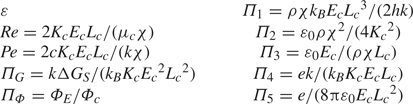
The equations include the 10 dimensionless numbers shown in table 2.
Table 1. Characteristic scales used to non-dimensionalize the equations.

Table 2. Dimensionless numbers parametrizing the solution.
3. Numerical solution
The system of equations is highly nonlinear and must be solved using an iterative scheme. Equations (2.26)–(2.39) are separated into groups solved sequentially, yielding an approximate solution that is iterated until convergence. We next describe these clusters of equations, relevant numerical methods and the solving scheme.
3.1. Electrostatic solution
The electric field, the surface charge and the flux of field-evaporated ions are computed by solving (2.29)–(2.33) which, after algebraic manipulations and discretization, are written as a single linear system of algebraic equations. First, we note that the right-hand sides of (2.29) and (2.30) are significant only near the tip of the meniscus, i.e. in regions 3 and 4, respectively. In these regions we solve the equations using finite differences in orthogonal grids (see Appendix A) using a second-order central difference for the space derivatives. In regions 1 and 2 these equations are well approximated by the Laplace equation, and solved using the boundary element method (BEM) (Brebbia & Dominguez Reference Brebbia and Dominguez1994; Brebbia, Telles & Wrobel Reference Brebbia, Telles and Wrobel2012; Bakr Reference Bakr2013). This method discretizes and solves the Laplace equation only on the boundary of the domain by converting it into the linear system  $\boldsymbol{\mathsf{H}}\boldsymbol {\varPhi }=\boldsymbol{\mathsf{G}}\boldsymbol {\varPhi }'$, where the potential and its normal derivative at the nodes of the discretized boundary are related by the $\boldsymbol{\mathsf{H}}$ and $\boldsymbol{\mathsf{G}}$ matrices computed with standard BEM techniques. Furthermore, on the surface of the meniscus we combine (2.31)–(2.33) to eliminate $J_\omega$ and $\sigma$ and obtain a single equation relating the normal components of the electric field on both sides of the surface, $E_n^i$ and $E_n^o$, as follows:
 \begin{align} E_n^i&=\dfrac{E_n^o}{\varepsilon+\dfrac{K}{2\varPi_3\left[\varPi_1 T\exp\left(\dfrac{G_E-\varPi_G}{T}\right)+\dfrac{t_r}{r}V_t+\dfrac{{\rm d}V_t}{{\rm d}t}\right]}}\nonumber\\ &\quad +\dfrac{\dfrac{{\rm d}\sigma}{{\rm d}t}V_t}{K+2\varepsilon\varPi_3\left[\varPi_1T\exp\left(\dfrac{G_E-\varPi_G}{T}\right)+\dfrac{t_r}{r}V_t+\dfrac{{\rm d}V_t}{{\rm d}t}\right]}. \end{align}
Here  $V_t$ is the surface tangential velocity and $t_r$ is the radial component of the tangential vector. This equation is written for simplicity as
 \begin{equation} E_n^i=B_E E_n^o+B_\sigma, \end{equation}
where the coefficients  $B_E$ and $B_{\sigma }$ are evaluated with the solution from the previous iteration.
The BEM applied to region 1 is written in matrix form as
 \begin{equation} \begin{bmatrix} \boldsymbol{\mathsf{H}}_{12} & \boldsymbol{\mathsf{H}}_{1o} & \boldsymbol{\mathsf{H}}_{14} & \boldsymbol{\mathsf{G}}_{12} & -\boldsymbol{\mathsf{G}}_{1c} & \boldsymbol{\mathsf{G}}_{14}\end{bmatrix}\begin{bmatrix} \boldsymbol{\varPhi}_{12}\\ \boldsymbol{\varPhi}_{1o}\\ \boldsymbol{\varPhi}_{14}\\ \boldsymbol{E}_n^o\\ \boldsymbol{E}_{1e}\\ \boldsymbol{E}_{1c}\\ \boldsymbol{E}_{14}\end{bmatrix}={-}\begin{bmatrix} \boldsymbol{\mathsf{H}}_{1e} & \boldsymbol{\mathsf{H}}_{1c} & \boldsymbol{\mathsf{G}}_{1o}\end{bmatrix}\begin{bmatrix} \boldsymbol{\varPhi}_{1e}\\ \boldsymbol{\varPhi}_{1c}\\ \boldsymbol{E}_{1o}\end{bmatrix}, \end{equation}
where the subindexes in all elements refer to the labelling of the boundaries in figure 1. The  $\boldsymbol {\varPhi }_{1e}$, $\boldsymbol {\varPhi }_{1c}$ and $\boldsymbol {E}_{1o}$ vectors are boundary conditions,
 \begin{equation} \boldsymbol{\varPhi}_{1e}=\varPi_\varPhi, \quad \boldsymbol{\varPhi}_{1c}=0, \quad \boldsymbol{E}_{1o} = 0. \end{equation}
The BEM applied to region 2 is written in matrix form as
 \begin{equation} \begin{bmatrix} \boldsymbol{\mathsf{H}}_{21} & \boldsymbol{\mathsf{H}}_{23} & \boldsymbol{\mathsf{G}}_{21} & -\boldsymbol{\mathsf{G}}_{2e} & -\boldsymbol{\mathsf{G}}_{23}\end{bmatrix}\begin{bmatrix} \boldsymbol{\varPhi}_{21}\\ \boldsymbol{\varPhi}_{23}\\ \boldsymbol{E}_n^i\\ \boldsymbol{E}_{2e}\\ \boldsymbol{E}_{23}\end{bmatrix}={-}\left[\boldsymbol{\mathsf{H}}_{2e}\right]\left[\boldsymbol{\varPhi}_{2e}\right], \end{equation}
with boundary condition
 \begin{equation} \boldsymbol{\varPhi}_{2e}=\varPi_\varPhi. \end{equation}
In region 3 equation (2.29) is written in the  $\{\xi _3,\eta _3\}$ orthogonal coordinate system using the relations defined in Appendix A:
 \begin{align} &\left(\dfrac{\partial\xi_3}{\partial x}^2+\dfrac{\partial\xi_3}{\partial r}^2\right)\dfrac{\partial^2\varPhi^i}{\partial{\xi_3}^2}+ \left(\dfrac{\partial\eta_3}{\partial x}^2+\dfrac{\partial\eta_3}{\partial r}^2\right)\dfrac{\partial^2\varPhi^i}{\partial{\eta_3}^2}+ \left(\dfrac{\partial^2\xi_3}{\partial x^2}+\dfrac{\partial^2\xi_3}{\partial r^2}+\dfrac{1}{r}\dfrac{\partial\xi_3}{\partial r}\right)\dfrac{\partial\varPhi^i}{\partial\xi_3}\nonumber\\ &\qquad +\left(\dfrac{\partial^2\eta_3}{\partial x^2}+\dfrac{\partial^2\eta_3}{\partial r^2}+\dfrac{1}{r}\dfrac{\partial\eta_3}{\partial r}\right)\dfrac{\partial\varPhi^i}{\partial\eta_3}={-}\dfrac{1}{K}\left[ \dfrac{\partial K}{\partial\xi_3}\left(\dfrac{\partial\xi_3}{\partial x}^2+\dfrac{\partial\xi_3}{\partial r}^2\right)\dfrac{\partial\varPhi^i}{\partial\xi_3}\right.\nonumber\\ &\qquad + \left. \dfrac{\partial K}{\partial\eta_3}\left(\dfrac{\partial\eta_3}{\partial x}^2+\dfrac{\partial\eta_3}{\partial r}^2\right)\dfrac{\partial\varPhi^i}{\partial\eta_3} \right]. \end{align}
This equation is discretized using finite differences and written in matrix form
 \begin{equation} \begin{bmatrix} \boldsymbol{\mathsf{M}}_3 & \boldsymbol{\mathsf{B}}_{34} & \boldsymbol{\mathsf{B}}_{23}\end{bmatrix}\begin{bmatrix} \boldsymbol{\varPhi}_{3}\\ \boldsymbol{\varPhi}_{34}\\ \boldsymbol{\varPhi}_{23}\end{bmatrix}=\left[\boldsymbol{F}_3\right], \end{equation}
where  $\boldsymbol{\mathsf{M}}_3$ and $\boldsymbol {F}_3$ are the matrix and the forcing term resulting from the discretization, while $\boldsymbol{\mathsf{B}}_{23}$ and $\boldsymbol{\mathsf{B}}_{34}$ are matrices associated with the matching of boundary conditions in the interfaces with regions 2 and 4, i.e. the electric potential and the normal component of the electric field are continuous across these interfaces. Matrix $\boldsymbol{\mathsf{M}}_3$ also contains the symmetry condition at the axis,
 \begin{equation} \frac{\partial\varPhi^3}{\partial r}(\xi_3,0)=0. \end{equation}
Similarly, (2.30) is solved in region 4 in an orthogonal grid and, after discretization, written as
 \begin{equation} \begin{bmatrix} \boldsymbol{\mathsf{M}}_4 & \boldsymbol{\mathsf{B}}_{43} & \boldsymbol{\mathsf{B}}_{41}\end{bmatrix}\begin{bmatrix} \boldsymbol{\varPhi}_{4}\\ \boldsymbol{\varPhi}_{34}\\ \boldsymbol{\varPhi}_{14}\end{bmatrix}={-}\left[\boldsymbol{\omega}\right], \end{equation}
where the matrix  $\boldsymbol{\mathsf{M}}_4$ contains the discretization of the equation and the boundary condition at the axis
 \begin{equation} \frac{\partial\varPhi^4}{\partial r}(\xi_4,0)=0 \end{equation}
while matrices  $\boldsymbol{\mathsf{B}}_{43}$ and $\boldsymbol{\mathsf{B}}_{41}$ contain the matching of boundary conditions between regions.
Equations (3.2), (3.3), (3.5), (3.8) and (3.10) are merged into a single linear system of algebraic equations to solve for the electric potential in regions 3 and 4,  $\boldsymbol {\varPhi }^3$ and $\boldsymbol {\varPhi }^4$, the electric potential on the surface of the meniscus, $\boldsymbol {\varPhi }_{12}$ and $\boldsymbol {\varPhi }_{34}$, and the normal components of the electric field on either side of the surface, $E_n^i$ and $E_n^o$. With this solution the tangential component of the electric field is computed by differentiating the electric potential along the surface, while the surface charge density is obtained from (2.31).
3.2. Fluid dynamic solution
The continuity and momentum equations, (2.26) and (2.27), are solved in the stream function-vorticity formulation, which in axisymmetric problems reduces the system of three coupled equations for the two velocity components and the pressure to a system of two coupled equations for the stream function  $\varPsi$ and the vorticity $\varOmega$,
 \begin{equation} \frac{\partial^2\varPsi}{\partial r^2}+ \frac{\partial^2\varPsi}{\partial x^2}-\frac{1}{r} \frac{\partial\varPsi}{\partial r}={-}r\varOmega, \end{equation}
 \begin{align} & \frac{\partial^2\varOmega}{\partial r^2}+\frac{\partial^2\varOmega}{\partial x^2}+\frac{1}{r}\frac{\partial\varOmega}{\partial r}-\frac{\varOmega}{r^2}=\frac{{{Re}}}{\mu r}\left(\frac{\partial\varPsi}{\partial r}\frac{\partial\varOmega}{\partial x}-\frac{\partial\varPsi}{\partial x}\frac{\partial\varOmega}{\partial r}+\frac{1}{r}\frac{\partial\varPsi}{\partial x}\varOmega\right)\nonumber\\ &\qquad -\frac{1}{\mu}\left[\frac{1}{r}\left(\frac{\partial^2\varPsi}{\partial x^2}-\frac{\partial^2\varPsi}{\partial r^2}+\frac{1}{r}\frac{\partial\varPsi}{\partial r}\right)\left(\frac{\partial^2\mu}{\partial r^2}-\frac{\partial^2\mu}{\partial x^2}\right)\right.\nonumber\\ &\qquad + \left.\frac{2}{r}\left(\frac{1}{r}\frac{\partial\varPsi}{\partial x}-2\frac{\partial^2\varPsi}{\partial x\partial r}\right)\frac{\partial^2\mu}{\partial x\partial r}+\frac{\partial\varOmega}{\partial x}\frac{\partial\mu}{\partial x}+\frac{\partial\varOmega}{\partial r}\frac{\partial\mu}{\partial r}\right], \end{align}
with
 \begin{gather} U=\frac{1}{r}\frac{\partial\varPsi}{\partial r}, \quad V={-}\frac{1}{r}\frac{\partial\varPsi}{\partial x}, \end{gather}
 \begin{gather} \boldsymbol{\varOmega}=\boldsymbol{\nabla}\times\boldsymbol{V}, \end{gather}
where  $U$ and $V$ are the axial and radial components of the velocity. Equations (3.12) and (3.15) are solved only in region 3, where the liquid velocity is expected to be significant, using the $\{\xi _3,\eta _3\}$ orthogonal coordinates defined in Appendix A,
 $$\begin{gather} \left(\frac{\partial\xi_3}{\partial x}^2+\frac{\partial\xi_3}{\partial r}^2\right)\frac{\partial^2\varPsi}{\partial{\xi_3}^2}+ \left(\frac{\partial\eta_3}{\partial x}^2+\frac{\partial\eta_3}{\partial r}^2\right)\frac{\partial^2\varPsi}{\partial{\eta_3}^2}+ \left(\frac{\partial^2\xi_3}{\partial x^2}+\frac{\partial^2\xi_3}{\partial r^2}-\frac{1}{r}\frac{\partial\xi_3}{\partial r}\right)\frac{\partial\varPsi}{\partial\xi_3}\nonumber\\ +\left(\frac{\partial^2\eta_3}{\partial x^2}+\frac{\partial^2\eta_3}{\partial r^2}-\frac{1}{r}\frac{\partial\eta_3}{\partial r}\right)\frac{\partial\varPsi}{\partial\eta_3}={-}r\varOmega, \end{gather}$$
 \begin{align} &\left(\frac{\partial\xi_3}{\partial x}^2+\frac{\partial\xi_3}{\partial r}^2\right)\frac{\partial^2\varOmega}{\partial{\xi_3}^2}+ \left(\frac{\partial\eta_3}{\partial x}^2+\frac{\partial\eta_3}{\partial r}^2\right)\frac{\partial^2\varOmega}{\partial{\eta_3}^2}+ \left(\frac{\partial^2\xi_3}{\partial x^2}+\frac{\partial^2\xi_3}{\partial r^2}+\frac{1}{r}\frac{\partial\xi_3}{\partial r}\right)\frac{\partial\varOmega}{\partial\xi_3}\nonumber\\ &\quad +\left(\frac{\partial^2\eta_3}{\partial x^2}+\frac{\partial^2\eta_3}{\partial r^2}+\frac{1}{r}\frac{\partial\eta_3}{\partial r}\right)\frac{\partial\varOmega}{\partial\eta_3}=\frac{{{Re}}}{r\mu}\left[\left(\frac{\partial\eta_3}{\partial x}\frac{\partial\xi_3}{\partial r}-\frac{\partial\xi_3}{\partial x}\frac{\partial\eta_3}{\partial r}\right)\left(\frac{\partial\varPsi}{\partial\xi_3}\frac{\partial\varOmega}{\partial\eta_3}-\frac{\partial\varPsi}{\partial\eta_3}\frac{\partial\varOmega}{\partial\xi_3}\right)\right.\nonumber\\ &\quad +\left.\left(\frac{\partial\xi_3}{\partial x}\frac{\partial\varPsi}{\partial\xi_3}-\frac{\partial\eta_3}{\partial x}\frac{\partial\varPsi}{\partial\eta}\right)\frac{\varOmega}{r}\right] +\frac{1}{\mu}\left[\frac{1}{r}\left(\frac{\partial^2\varPsi}{\partial x^2}-\frac{\partial^2\varPsi}{\partial r^2}+\frac{1}{r}\frac{\partial\varPsi}{\partial r}\right)\left(\frac{\partial^2\mu}{\partial x^2}-\frac{\partial^2\mu}{\partial r^2}\right)\right.\nonumber\\ &\quad + \left.\frac{2}{r}\left(\frac{2\partial^2\varPsi}{\partial x\partial r}-\frac{1}{r}\frac{\partial\varPsi}{\partial x}\right)\frac{\partial^2\mu}{\partial x\partial r}- \left(\frac{\partial\xi_3}{\partial x}^2+\frac{\partial\xi_3}{\partial r}^2\right)\frac{\partial\varOmega}{\partial\xi_3}\frac{\partial\mu}{\partial\xi_3}+ \left(\frac{\partial\eta_3}{\partial x}^2+\frac{\partial\eta_3}{\partial r}^2\right)\frac{\partial\varOmega}{\partial\eta_3}\frac{\partial\mu}{\partial\eta_3}\right], \end{align}
where the last terms are given in  $\{x,r\}$ coordinates for brevity. The equations, discretized using finite differences, fulfil the boundary conditions
 \begin{gather} \left. \begin{gathered} \varPsi(\xi_3,0)=0 \quad \frac{\partial\varPsi}{\partial\xi_3}(\xi_3,1)=\dfrac{-rJ_\omega}{2\sqrt{\dfrac{\partial\xi_3}{\partial x}^2+\dfrac{\partial\xi_3}{\partial r}^2}}\\ \dfrac{\partial\varPsi}{\partial\xi_3}(0,\eta_3)=0 \quad \varPsi(1,\eta_3)=0 \end{gathered} \right\}, \end{gather}
 \begin{gather} \left. \begin{gathered} \varOmega(\xi_3,0)=0 \quad \varOmega(\xi_3,1)=\dfrac{{{Re}}\varPi_2}{2\varPi_3}\dfrac{E_t\sigma}{\mu}-\dfrac{2}{r}\left[\dfrac{1}{t_x}\dfrac{\partial t_r}{\partial t}\dfrac{\partial\varPsi}{\partial n}-\dfrac{t_r}{r}\dfrac{\partial\varPsi}{\partial t}+\dfrac{\partial^2\varPsi}{\partial t^2}\right]\\ \frac{\partial\varOmega}{\partial\xi_3}(0,\eta_3)=0 \quad \varOmega(1,\eta_3)=0 \end{gathered} \right\}. \end{gather}
The linear systems of algebraic equations for the stream function and the vorticity resulting from the discretization and application of boundary conditions are solved separately to improve numerical stability. The boundary condition for the vorticity on the surface of the meniscus is derived from (2.39), and links the fluid dynamic and the electrostatic problems. The balance of tangential stresses on the surface is the main driver of the liquid flow, while the outward velocity due to ion emission has a smaller contribution (the flow rates of ion-emitting Taylor cones are low).
3.3. Fluid temperature and the variation of physical properties
The temperature can be written as  $T(x, r)=T_0 + T_1(x, r)$, where $T_0$ is the upstream temperature. We solve (2.28) for $T_1(x,r)$ in region 3, using the $\{\xi _3,\eta _3\}$ orthogonal coordinates
 \begin{align} &\left(\frac{\partial\xi_3}{\partial x}^2+\frac{\partial\xi_3}{\partial r}^2\right)\frac{\partial^2T_1}{\partial{\xi_3}^2}+ \left(\frac{\partial\eta_3}{\partial x}^2+\frac{\partial\eta_3}{\partial r}^2\right)\frac{\partial^2T_1}{\partial{\eta_3}^2}+ \left(\frac{\partial^2\xi_3}{\partial x^2}+\frac{\partial^2\xi_3}{\partial r^2}+\frac{1}{r}\frac{\partial\xi_3}{\partial r}\right)\frac{\partial T_1}{\partial\xi_3}\nonumber\\ &\quad +\left(\frac{\partial^2\eta_3}{\partial x^2}+\frac{\partial^2\eta_3}{\partial r^2}+\frac{1}{r}\frac{\partial\eta_3}{\partial r}\right)\frac{\partial T_1}{\partial\eta_3}={-}\frac{Pe}{r}\left(\frac{\partial\xi_3}{\partial x}\frac{\partial\eta_3}{\partial r}+\frac{\partial\eta_3}{\partial x}\frac{\partial\xi_3}{\partial r}\right)\left(\frac{\partial\varPsi}{\partial\xi}\frac{\partial T_1}{\partial\eta}-\frac{\partial\varPsi}{\partial\eta}\frac{\partial T_1}{\partial\xi}\right)\nonumber\\ &\quad -\frac{2\varPi_3}{{{Re}}\varPi_2}\frac{\mu}{r^2}\left[2\frac{\partial^2\varPsi}{\partial x\partial r}^2+\left(\frac{\partial^2\varPsi}{\partial r^2}-\frac{\partial^2\varPsi}{\partial x^2}-\frac{1}{r}\frac{\partial\varPsi}{\partial r}\right)^2+2\left(\frac{\partial^2\varPsi}{\partial x\partial r}-\frac{1}{r}\frac{\partial\varPsi}{\partial x}\right)^2\right]\nonumber\\ &\quad -K\left[\left(\frac{\partial\xi_3}{\partial x}^2+\frac{\partial\xi_3}{\partial r}^2\right)\frac{\partial\varPhi^i}{\partial\xi_3}^2+\left(\frac{\partial\eta_3}{\partial x}^2+\frac{\partial\eta_3}{\partial r}^2\right)\frac{\partial\varPhi^i}{\partial\eta_3}^2\right], \end{align}
where several stream function terms in the right-hand side are written in  $\{x,r\}$ coordinates for brevity. The boundary conditions for the temperature field are
 \begin{equation} \left. \begin{gathered} \frac{\partial T_1}{\partial\eta_3}(\xi_3,0)=0 \quad \frac{\partial T_1}{\partial\eta_3}(\xi_3,1)=0\\ T_1(0,\eta_3)=0 \quad \frac{\partial T_1}{\partial\xi_3}(1,\eta_3)=0 \end{gathered} \right\}. \end{equation}
The temperature equation (3.20) is discretized using finite differences, resulting in a linear system of algebraic equations that incorporates the boundary conditions. The solution for the temperature field is then used to compute the viscosity and conductivity near the tip of the meniscus, using (2.5) and (2.6).
3.4. Ion beam
We compute the density and velocity fields of the ion beam by integrating the equations of conservation of mass (2.36) and momentum (2.37),
 \begin{gather} u\frac{\partial\omega}{\partial x}+v\frac{\partial\omega}{\partial r}+\omega\left(\frac{\partial u}{\partial x}+\frac{\partial v}{\partial r}+\frac{v}{r}\right)=0, \end{gather}
 \begin{gather} \left. \begin{aligned} u\frac{\partial u}{\partial x}+v\frac{\partial u}{\partial r} & ={-}\varPi_2\varPi_3\frac{\partial\varPhi^o}{\partial x},\\ u\frac{\partial v}{\partial x}+v\frac{\partial v}{\partial r} & ={-}\varPi_2\varPi_3\frac{\partial\varPhi^o}{\partial r}, \end{aligned} \right\} \end{gather}
using the method of characteristics. The distance along the trajectory of an ion is defined as the new coordinate of integration,
 \begin{equation} \frac{{\rm d}}{{\rm d}s}=\frac{\partial x}{\partial s}\frac{\partial}{\partial x}+\frac{\partial r}{\partial s}\frac{\partial}{\partial r}, \end{equation}
and, using this new coordinate, the equations are rewritten as
 \begin{equation} \left. \begin{gathered} \frac{{\rm d}u}{{\rm d}s}={-}\varPi_2\varPi_3\frac{\partial\varPhi^o}{\partial x} \quad \frac{{\rm d}v}{{\rm d}s}={-}\varPi_2\varPi_3\frac{\partial\varPhi^o}{\partial r},\\ \frac{{\rm d}\omega}{{\rm d}s}=\omega\left[\frac{\varPi_2\varPi_3}{u^2+v^2}\left(u\frac{\partial\varPhi^o}{\partial x}+v\frac{\partial\varPhi^o}{\partial r}\right)-\frac{1}{u^2+v^2}\left(u\frac{\partial v}{\partial p}-v\frac{\partial u}{\partial p}\right)-\frac{v}{r}\right], \end{gathered} \right\} \end{equation}
where  $p$ is the coordinate normal to $s$. Characteristic lines are obtained by integrating
 \begin{equation} \frac{\partial x}{\partial s}=u \quad {\rm and} \quad \frac{\partial r}{\partial s}=v. \end{equation}
The initial positions of the characteristic lines coincide with the surface of the meniscus, while the initial value of the ion density is obtained from the emitted current density and the initial ion velocity,
 \begin{equation} \omega_0=\frac{J_\omega}{\chi\left\|\boldsymbol{v}_0\right\|}. \end{equation}
We estimate the initial ion velocity  $\boldsymbol {v}_0$ as the average velocity of the ions that can escape the energy barrier,
 \begin{equation} v_{avg}=\frac{\displaystyle\int_{\Delta G}^\infty{v f_M(v)}\,{\rm d}v}{\displaystyle\int_{\Delta G}^\infty{f_M(v)}\,{\rm d}v}, \end{equation}
where  $\Delta G={\Delta G}_S-G_E$ is the local value of the energy barrier. The ion population in the meniscus is in thermal equilibrium and therefore characterized by a Maxwellian distribution $f_M(v)$. A good estimate for the initial velocity of the ions is that associated with (3.28), reduced by the climb of the energy barrier. In dimensionless quantities, the resulting initial ion density and velocity are
 \begin{equation} \left. \begin{gathered} \omega_0=\dfrac{J_\omega}{2\chi\left\|\boldsymbol{v}_0\right\|},\\ \left\|\boldsymbol{v}_0\right\|=\sqrt{\dfrac{T}{m}\left[\dfrac{2\left(\dfrac{\Delta G}{T}+1\right)}{2\sqrt{\dfrac{\Delta G}{T}}+\sqrt{\rm \pi}\exp\left(\dfrac{\Delta G}{T}\right)\operatorname{erfc}\sqrt{\dfrac{\Delta G}{T}}}\right]^2-\dfrac{2\Delta G}{m}}. \end{gathered} \right\} \end{equation}
3.5. Pressure in the meniscus
The pressure field in the meniscus is needed to enforce the equilibrium of normal stresses, (2.38). The pressure along the surface is computed by integrating the momentum equation using the latest solution for the velocity field. Equation (2.27) is first multiplied by the vector  $\boldsymbol {t}$ tangential to the surface
 \begin{align} \frac{\partial}{\partial t}\left(\frac{\cos\theta_T}{\varPi_2}\boldsymbol{V}\boldsymbol{\cdot}\boldsymbol{V}+P\right)=\frac{2\cos\theta_T}{\varPi_2}\left[\boldsymbol{V}\times\boldsymbol{\varOmega}+\frac{\mu\nabla^2\boldsymbol{V}+\left(\boldsymbol{\nabla}\boldsymbol{V}+{\boldsymbol{\nabla}\boldsymbol{V}}^{\rm T}\right)\boldsymbol{\cdot}\boldsymbol{\nabla}\mu}{{{Re}}}\right]\boldsymbol{\cdot}\boldsymbol{t}. \end{align}
This equation is then converted into the surface reference frame  $\{t,n\}$ defined in Appendix A, and integrated. All terms containing ${\partial \mu }/{\partial n}$ are zero due to the boundary condition for the temperature field on the surface. The final expression for the pressure along the surface is
 \begin{align} P&=P_{tip}+\frac{2\cos\theta_T}{\varPi_2}\left[\int_0^t{\frac{\partial\varPsi}{\partial t}\frac{\varOmega}{r}}\,{\rm d}t -\frac{1}{2r^2}\left(\frac{\partial\varPsi}{\partial t}^2+\frac{\partial\varPsi}{\partial n}^2\right)\right]\nonumber\\ &\quad +\frac{2\cos\theta_T}{{{Re}}\varPi_2}\int_0^t{\mu\left(\frac{\partial\varOmega}{\partial n}-\frac{\varOmega t_x}{r}\right)+\frac{2}{r}\frac{\partial\mu}{\partial t}\left(\frac{1}{t_x}\frac{\partial t_r}{\partial t}\frac{\partial\varPsi}{\partial t}+\frac{t_r}{r}\frac{\partial\varPsi}{\partial n}-\frac{\partial^2\varPsi}{\partial t\partial n}\right)}\,{\rm d}t, \end{align}
where  $P_{tip}$ is the pressure at the tip of the meniscus. The surface coordinate $t$ starts at the tip of the meniscus and progresses along the surface up to the emitter. Once the integration is performed, $P_{tip}$ is adjusted so that the pressure at the emitter matches the upstream condition $P=P_0$ (we set $P_0 = 0$).
3.6. Surface optimization
The position of the surface of the meniscus is computed in each iteration by minimizing the error in the balance of normal stresses. To do so (2.38) is written as
 $$\begin{gather} \frac{1}{\sqrt{\varrho^2+{\varrho'}^2}}\left(\frac{\varrho\varrho''-{\varrho'}^2}{\varrho^2 +{\varrho'}^2}+\frac{\varrho'}{\varrho\tan\theta}-2\right)={-}P-\cos\theta_T\left[{E_n^o}^2-\varepsilon{E_n^i}^2+\left(\varepsilon-1\right){E_t}^2\right]\nonumber\\ +\, \frac{4\cos\theta_T}{{{Re}}\varPi_2}\frac{\mu}{r}\left(\frac{1}{n_r}\frac{\partial n_r}{\partial n}\frac{\partial\varPsi}{\partial n}+\frac{t_x}{r}\frac{\partial\varPsi}{\partial t}+\frac{\partial^2\varPsi}{\partial t\partial n}\right), \end{gather}$$
where the left-hand side is the surface tension stress written in terms of the position of the surface in polar coordinates  $\varrho =\varrho (\theta )$. The right-hand side of (3.32) is evaluated with the latest solution. This formulation in polar coordinates (originating at the tip of the emitter, see Appendix B) avoids numerical instabilities both at the vertex of the meniscus ( $\theta =0$) and at the anchoring point, $\theta ={\rm \pi} /2$. The use of Cartesian coordinates would result in very large or infinite derivatives at these points. The apparent singularity at $\theta =0$ in the $\varrho '/\varrho \tan \theta$ term is resolved with a Taylor expansion of $\varrho '$ in the vicinity of the vertex, which shows the term to be finite for a tip with a finite radius of curvature,
 \begin{equation} \lim_{\theta\rightarrow 0}{\frac{\varrho'}{\varrho\tan\theta}}=\lim_{\theta\rightarrow 0}{\frac{\varrho'(0)+\varrho''(0)\theta}{\varrho\theta}}=\frac{\varrho''(0)}{\varrho(0)}. \end{equation}
Equation (3.32) is used to optimize the surface by applying the integral least-square technique. The residual along the surface is defined as
 \begin{gather} \mathcal{E}=\frac{1}{2}\int_0^{{\rm \pi}/2}f^2(\varrho(\theta),y(\theta),\theta)+\left(\varrho'-y\right)^2 \,{\rm d}\theta, \end{gather}
 $$\begin{gather} f(\varrho,y,\theta)=\frac{\varrho y'-y^2}{\varrho^2+y^2}+\frac{y}{\varrho\tan\theta}-2+\sqrt{\varrho^2+y^2}\left\{\cos\theta_T\left[{E_n^o}^2-\varepsilon{E_n^i}^2+\left(\varepsilon-1\right){E_t}^2\right]\right.\nonumber\\ +\left. P-\frac{4\cos\theta_T}{{{Re}}\varPi_2}\frac{\mu}{r}\left(\frac{1}{n_r}\frac{\partial n_r}{\partial n}\frac{\partial\varPsi}{\partial n}+\frac{t_x}{r}\frac{\partial\varPsi}{\partial t}+\frac{\partial^2\varPsi}{\partial t\partial n}\right)\right\}, \end{gather}$$
where the first derivative  $\varrho '$ has been converted into a second optimization variable $y$ to improve the stability of the algorithm. To minimize the residual $\mathcal {E}$, the surface is discretized with the same set of nodes used for the electrostatic problem, and the resulting integration provides two equations at each point $j$ for the surface position $\varrho _j$ and its first derivative $y_j$,
 \begin{gather} \int_0^{{\rm \pi}/2}f\frac{\partial f}{\partial\varrho_j}+\left(\varrho'-y\right)\frac{\partial\varrho'}{\partial\varrho_j}\,{\rm d}\theta=0, \end{gather}
 \begin{gather} \int_0^{{\rm \pi}/2}f\frac{\partial f}{\partial y_i}+\left(\varrho'-y\right)\frac{\partial\varrho'}{\partial y_j}\,{\rm d}\theta=0. \end{gather}
This system of algebraic equations is solved using the Newton's method. Regions 3 and 4 are redefined in each iteration with the updated surface. The transition between regions 2 and 3 is set at the point in the surface where the ion current density drops to  $10^{-12}$ of its maximum which, due to the exponential nature of the ion emission law, is always near the vertex of the meniscus; and the transition between regions 1 and 4 is set at the axial point where the ion density drops to $10^{-8}$ of its maximum.
3.7. Breakdown of the continuum hypothesis near the vertex of the meniscus
Ion emission is localized in a small region surrounding the tip of the meniscus. The continuum hypothesis breaks down within a distance from the vertex of a few molecular radii (for the ionic liquids of interest in this study, the molecular radius if approximately one half of a nanometre), and we do not expect nor require the model equations to be accurate in this molecular-size region. Instead, we define a Knudsen number in terms of the distance  $\delta$ from the vertex of the meniscus
 \begin{equation} K_n=\frac{\lambda_m}{2\delta}=\frac{1}{\delta}\left(\frac{3 m}{4{\rm \pi}\rho}\right)^{1/3}, \end{equation}
where the mean free path  $\lambda _m$ has been expressed in terms of the molecular mass $m$ and the liquid density, use a critical value of the Knudsen number to define the extent of the region where the continuum hypothesis breaks down, and extrapolate the continuum solution into this region by using a patching function that preserves axial symmetry
 \begin{equation} \mathcal{F}(\delta<\delta_K)=\mathcal{F}(\delta_K)+\frac{\mathcal{F}'(\delta_K)}{2}\left(\frac{\delta^2}{\delta_K}-\delta_K\right). \end{equation}
Here  $\delta _K$ is the position on the surface where the Knudsen number reaches the critical value. We typically adopt a critical value of 0.1 for the Knudsen number, or equivalently $\delta _K=3.93$ nm, and use (3.39) to evaluate the stream function, the vorticity, the pressure and the viscous stress near the vertex.
3.8. Solving scheme
The input parameters in the model are the radius of the emitter, the distance and the potential difference between the emitter and the extractor electrode, the physical properties of the liquid and the upstream temperature. The pressure jump  $P_0$ across the surface is set to zero at the anchor point on the emitter. The solution of the model provides the shape of the meniscus; the velocity, pressure and temperature fields in the liquid phase; the electric field and surface charge; and the density and velocity fields of the ion beam. Figure 3 shows a flow chart of the algorithm used to solve the system of equations. First, we make a guess for the shape of the meniscus, assume a zero velocity field and a constant temperature throughout the fluid. With these values we start the iterative procedure: the sizes of regions 3 and 4 are determined (in the first iteration we use $10\times L_c$ as initial guess); the boundaries of the four regions are discretized and the orthogonal grids of regions 3 and 4 computed. The grid discretizations of regions 3 and 4 have $100\times 50$ and $50\times 100$ points, respectively, with higher point density near the tip of the meniscus and close to the surface of the liquid (see Appendix A). The boundary of region 1 is discretized using 1400 points, while region 2 uses 1100 points. One thousand of these points are shared between the two regions, and are used to discretize the portion of the surface not included in the orthogonal grids of regions 3 and 4. The boundary elements of this portion of the surface have variable size for a smooth transition between the spacing of the orthogonal grids and the rest of the domain discretization. The electric problem, the fluid dynamic problem and the temperature equation are solved in this order; the viscosity and electrical conductivity are updated with the computed temperature field; and the ion beam is computed. These steps are iterated until convergence of the total ion current. At this point the residual of the surface normal stresses is evaluated and if it is below a specified threshold, typically $10^{-5}$, the solution is accepted as final, otherwise the surface is modified using (3.36) and (3.37) and, with the updated shape of the meniscus, a new iteration is started.

Figure 3. Flow chart of the algorithm for solving the system of equations.
4. Simulation results and discussion
We study ion emission from the ionic liquid 1-ethyl-3-methylimidazolium tetrafluoroborate, [C $_2$C
$_2$C $_1$Im][BF $_4$], which is known to operate in ion emission regime (Romero-Sanz et al. Reference Romero-Sanz, Bocanegra, Fernández De La Mora and Gamero-Castaño2003; Lozano & Martinez-Sanchez Reference Lozano and Martinez-Sanchez2005a). The physical properties of [C $_2$C
$_2$C $_1$Im][BF $_4$] are taken from the National Institute of Standards and Technology (NIST) ionic liquid database (Kazakov et al. Reference Kazakov, Magee, Chirico, Paulechka, Diky, Muzny, Kroenlein and Frenkel2022), see table 3. The upstream values of the pressure and temperature are fixed at 0 Pa and $25\,^\circ$C; the diameter of the emitter is 40 $\mathrm {\mu }$m; the distance between the emitter and extractor is 1 mm; the potential difference between the emitter and extractor electrodes is varied between 1600 and 2200 V; and the ion solvation energy is varied between 1.2 and 1.9 eV. The associated values of the dimensionless numbers, shown in table 4, illustrate the relative importance of several terms in the governing equations: the Reynolds number is small, indicating Stokes flow conditions; the small value of $2\varPi _3/({{Re}}\varPi _2)$ in (2.28) indicates that viscous dissipation is small compared with ohmic dissipation; the values of $\varPi _G$, increasing of one order of magnitude from ${\Delta G}_S=1.2$ eV to ${\Delta G}_S=1.9$ eV, denote the increasing difficulty for the ions to overcome the energy barrier; and the large value of $\varPi _1$ denotes the sensibility of ion emission to changes in the energy barrier and temperature.
Table 3. Physical properties of [C $_2$C
$_2$C $_1$Im][BF $_4$] at $25\,^\circ$C. The electrical conductivity and the viscosity are given as functions of the temperature.

Table 4. Values of the dimensionless numbers for [C $_2$C
$_2$C $_1$Im][BF $_4$] at $T = 25\,^\circ$C and $\varPhi _E=1900$ V, and several values of the ion solvation energy.

Figure 4 shows the velocity field in region 3 and an inset with the overall shape of the meniscus, for  $\varPhi _E = 1900$ V and ${\Delta G}_S = 1.7$ eV. The electro-hydrostatic region 2 occupies most of the meniscus, while dynamical processes associated with ion emission only affect a small area near the vertex. The module of the velocity is small everywhere in region 3 except near the vertex, where the liquid flows outward and is emitted as ions. Regardless of the magnitude increase near the tip, the velocity is relatively uniform perpendicularly to the streamlines and the flow does not have a sharp redirection as it moves towards the surface. The resulting viscous stresses and viscous dissipation remain small. While the flow is smooth and uniform near the tip, a flow recirculation zone, also observed by Gallud & Lozano (Reference Gallud and Lozano2022), extends over most of the meniscus. In the ion emission regime the flow rate is strongly coupled to the current emitted in the form of ions. In the present model the ion current and the liquid flow rate are proportional, with a constant of proportionality fixed by the charge-to-mass ratio of the ion. In a real scenario the ions exhibit a distribution of solvation states, which may slightly alter the proportionality between the emitted ion current and the liquid flow rate if the distribution changes with the emitted current.

Figure 4. Shape of the meniscus and magnitude of the liquid velocity and streamlines in region 3, for  $\varPhi _E = 1900$ V and ${\Delta G}_S = 1.7$ eV. The red line marks $K_n = 0.1$. The values of the characteristic velocity and length are $V_{fc} = 4.15\,\textrm {m}\,\textrm {s}^{-1}$ and $L_c = 2.77$ nm.
Figure 5 shows the components of the normal stress on the surface of the meniscus. The dominant terms are the surface tension and electric stresses, which are in almost complete balance throughout the surface, while the pressure and viscous stresses become marginally important only near the vertex, coinciding with the area of significant ion emission. It is worth noting that the ideal Taylor cone is also characterized by a perfect balance between surface tension and electric stresses. The balance of normal stresses, i.e. the residual of the numerical solution, is negligible throughout the surface except very close to the tip, within a distance from the vertex where the continuum hypothesis breaks down. For example, the residue is between 5 % and 8 % of the surface tension stress within 3 nm from the vertex.

Figure 5. Components of the normal stress on the surface of the meniscus for  $\varPhi _E = 1900$ V and ${\Delta G}_S = 1.7$ eV ( $L_c=2.77$ nm).
Figure 6 plots components of the electric field on the surface of the meniscus, together with the ratio between the current density of emitted ions and the current injected from the bulk. Here  $E_n^o$ is the dominant component everywhere, while the tangential component $E_t$ is at least two orders of magnitude smaller except near the vertex, where $E_t/E_n^o$ has a maximum value between 0.1 and 0.15 for the cases investigated. Thus, the meniscus is nearly equipotential. Here $E_n^i$ is negligible throughout most of the meniscus, but near the tip it reaches its maximum possible value, $E_n^i \cong E_n^o /\varepsilon$, corresponding to the absence of surface charge. The ratio $J_\omega /KE_n^i$ is near zero throughout most of the meniscus, and increases sharply towards one near the vertex, coinciding with the changes in the trends of the $E_t$ and $E_n^i$ components. The two distinct behaviours of $J_\omega /KE_n^i$ confirm the relative importance of the transport mechanisms described in § 2.3: upstream, far from the vertex, the smallness of $E_n^o$ and the associated high energy barrier for ion emission is the restrictive mechanism, and conduction from the bulk supplies current to the surface at rates orders of magnitude larger than the emitted current; near the vertex, current conduction from the bulk is the limiting transport mechanism, restricting the emitted current to what is injected from the bulk.

Figure 6. Components of the electric fields and ratio  $J_\omega /KE_n^i$ on the surface of the meniscus, for $\varPhi _E = 1900$ V and ${\Delta G}_S = 1.7$ eV ( $L_c=2.77$ nm).
Figure 7 shows the ion current density  $J_\omega$, the accumulated ion current (the integral of the current density over the surface of the meniscus),
 \begin{equation} I_I(x)=2{\rm \pi}\int_{x}^{x_E}{R\sqrt{1+R'^2}J_\omega}{{\rm d} x}, \end{equation}
and an estimate of the accumulated ion current based on the value of the outer the electric field and the assumption of an equipotential meniscus, i.e.  $\sigma = E_n^o/\varepsilon _0$,
 \begin{equation} I_{I\sigma}(x)=\frac{2{\rm \pi} k_B\varepsilon_0}{h}\int_{x}^{x_E}{R\sqrt{1+R'^2} E_n^o T\exp\left(\frac{G_E-{\Delta G}_S}{k_B T}\right)}{{\rm d} x}. \end{equation}
The current density profiles have the structure predicted by the simple model for the ideal Taylor cone, (2.20), namely ion emission is negligible throughout most of the meniscus and increases rapidly towards the vertex, reaching a point where further increase is strongly limited by bulk conduction. This abrupt change in the growth of the current density profile, and the similar shape of the associated profile for the accumulated current, show the presence of a distinct region near the vertex where most of the emission takes place, and make it possible to define a characteristic length for this region. The prediction of a characteristic length for the ion emission region is thus qualitatively correct, and we will show later in this section that the scaling (2.23) for  $L_c$ is also quantitatively accurate. Figure 7 also illustrates the importance of considering the transport mechanisms inside the meniscus, especially near the vertex, since a simpler estimation of emission using the equipotential solution overestimates the total ion current by several orders of magnitude. For the larger value of the ion solvation energy the ion current departs from $I_{I\sigma }$ at a position slightly larger than $x/L_c=1$. Only for the lowest values of the solvation energy investigated the curves diverge significantly upstream of $x/L_c=1$. We will show that this is due to large increases of the temperature near the tip, and the inaccurate evaluation of $L_c$ based on the upstream temperature.

Figure 7. Emitted current density  $J_\omega$, total emitted current $I_I$, and estimated total current for an equipotential meniscus $I_{I\sigma }$, for $\varPhi _E = 1900$ V and two values of the ion solvation energy.
The potential drop along the meniscus is negligible despite intense ion emission. The small tangential component of the electric field in figure 6 hints at this, and the potential profiles in figure 8 explicitly illustrate this point. This figure shows the variation of the potential along the surface of the meniscus for three different values of the solvation energy and two values of the emitter potential. In all cases the variation of the potential is small, it occurs mostly near the vertex and increases at decreasing  ${\Delta G}_S$ due to the intensification of ion emission.

Figure 8. Variation of the electric potential along the meniscus for several emitter potentials and ion solvation energies.
Energy dissipation and the associated increase of the temperature in the meniscus are important. Figure 9 shows an example of the temperature field in region 3, for  ${\Delta G}_S = 1.7$ eV and $\varPhi _E = 1900$ V. The temperature at the tip is $21\,^\circ$C higher than at the inlet. Dissipation concentrates near the vertex, ohmic dissipation being the main contributor; this term is proportional to $J^2$, and the current density exhibits a sharp maximum at the tip due to the emission of ions from this small region. In this particular case the ratio between ohmic and viscous dissipation near the tip has an average of 86.9, with peaks of over 900. Ion emission drives the flow field and the electric current in the meniscus, and therefore the energy dissipation and the increase in temperature. There is positive feedback: ion emission increases dissipation and the temperature, which increases the conductivity of the liquid and the availability of ions that can be injected on the surface. The larger thermal energy of the ions and therefore the larger number of ions that can overcome the energy barrier impeding emission is a second mechanism for positive feedback. However, conduction through the bulk is the limiting process for the emission of ions near the tip, (2.22), and therefore the larger thermal energy is less important than the increased electrical conductivity. On the other hand, the larger thermal energy of the ions has a small effect on the size of the emission region through the factor $\alpha$ in (2.23).

Figure 9. Temperature increase in region 3 for  $\varPhi _E = 1900$ V and ${\Delta G}_S = 1.7$ eV. The red line marks $K_n = 0.1$.
Figure 10 shows the effect of the emitter potential on the total emitted current for two values of the solvation energy. The current increases linearly with the emitter potential, and exhibits a strong dependence on the solvation energy. The proportionality between the emitted current and  $\varPhi _E$, reported in experiments by Krpoun & Shea (Reference Krpoun and Shea2008), can be inferred from (2.22). The current density near the vertex of the meniscus is proportional to the intensity of the electric field, and therefore to the potential of the emitter in a finite, physical configuration. Since the size of the emission region is only a function of the physical properties of the liquid and a weak function of the temperature, (2.23), the total emitted current must be approximately proportional to $\varPhi _E$.

Figure 10. Emitted ion current vs emitter potential for two values of the solvation energy.
Figure 11 shows the effect of the ion solvation energy on both the total ion current and the temperature near the vertex of the meniscus, for  $\varPhi _E=1900$ V. Reducing the solvation energy strongly increases the ion current because of the positive feedback between emission and temperature, and the expansion of the emission area. The temperature in the emission region increases rapidly with decreasing solvation energy. Values exceeding a few hundred centigrade degrees are non-physical, because the model does not take into account phenomena such as liquid evaporation and degradation which are important at elevated temperatures. Still, these trends suggest that the rapid temperature increase and the associated degradation of the liquid prevents steady ion emission for ion–liquid systems with low solvation energies, e.g. ${\Delta G}_S \lesssim 1.5\unicode{x2013} 1.4$ eV.

Figure 11. Effect of the ion solvation energy on the current of emitted ions and the tip temperature ( $\varPhi _E = 1900$ V).
The characteristic length of the ion emission area, (2.23), was introduced with the caveat that the simple model may be inaccurate near the vertex of the meniscus. Thus, although the existence of this emission region is confirmed by the current density profiles shown in figure 7, the scaling (2.23) needs to be verified. Figure 12 shows the radius of the base of the cusp from which 70 % and 95 % of the ion current is emitted,  $r_{70\,\%}$ and $r_{95\,\%}$, respectively, as a function of the solvation energy and for $\varPhi _E = 1900$ V. The radius of the region from which most ions are emitted ranges between 2.96 nm for ${\Delta G}_S = 1.9$ eV, and 82.0 nm for ${\Delta G}_S = 1.2$ eV. Figure 12 also shows the ratio $L_c/r_{70\,\%}$, where we use the temperature upstream $T_0$ to evaluate $L_c$. Here $L_c/r_{70\,\%}$ is near one for ${\Delta G}_S \geq 1.4$ eV and decreases rapidly for lower solvation energies. Thus, the scaling law (2.23) provides an accurate estimate of the size of the emission region, except for solvation energies unphysically low. The ratio $L_c/r_{70\,\%}$ is smaller than one for low solvation energies because we use the upstream temperature to evaluate $L_c$, instead of the temperature at the tip which is significantly higher than $T_0$ for low solvation energies.

Figure 12. Radius of the emission region from which 70 % and 95 % of the ion current is emitted, and ratio between the characteristic length of the emission region and the computed value.
The scaling laws for the current density and the size of the emission region, (2.22) and (2.23), make it possible to derive a scaling law for the emitted current,  $I_c \cong 2{\rm \pi} L_{c}^2J_\omega$ where we approximate the emission area by a hemisphere of radius $L_c$,
 \begin{equation} I_c=\frac{\cos^2{\theta_T}}{8{\rm \pi}}\frac{\alpha^{3/2} q^9K\gamma^2}{{\varepsilon_0}^5\varepsilon{{\Delta G}_S}^6}. \end{equation}
To estimate the current density, (2.22), we use the electric field of the ideal Taylor cone evaluated at  $r= L_c$,
 \begin{equation} E_c=\sqrt{2\gamma\cos\theta_T/(\varepsilon_0 L_c)}. \end{equation}
Note that the scaling law (4.3) does not include the effect of the emitter potential for a given liquid and electrode geometry illustrated by figure 10. The scaling law (4.3) is an analytical expression, and including the effect of the emitter potential requires a numerical calculation. Figure 13 shows the ratio between the scaling law and the current values obtained in the simulations. When the upstream temperature is used to evaluate (4.3), the scaling law reproduces the computed current for  ${\Delta G}_S \geq 1.6$ eV and underestimates the current at lower solvation energy. The agreement extends to lower solvation energies when the temperature at the tip is used to evaluate the scaling law (although this defeats the purpose of the scaling law because the numerical solution is needed to compute the tip temperature). Overall, the scaling law for the emitted current (4.3) highlights the importance of the solvation energy, and the lesser but significant roles of the electrical conductivity and the surface tension.

Figure 13. Ratio between the emitted current derived from scaling law (4.3) and the current computed with the simulations, for  $\varPhi _E = 1900$ V. The scaling law is evaluated with the upstream temperature (green), and with the temperature at the tip of the meniscus (blue).
The electrosprays of some ionic liquids operate in the ion emission regime, while other ionic liquids with similar physical properties only operate in the cone-jet mode. The results presented in this article, in particular the finding of a distinct emission region with characteristic size  $L_c$ and electric field $E_c$, may explain this and provide a criterion for the onset of the ion emission regime. Electrosprays operating in the cone-jet mode approximate well the ideal Taylor cone: most of the meniscus of a cone-jet is virtually electrostatic and hydrostatic (the local angle of the surface may depart from $\theta _T$ due to the finite size of the emitter and the space charge of the beam), and the main difference occurs at the tip which transitions into a jet. Here $E_n^o$ departs from the ideal Taylor cone solution in this transition region, where it exhibits a maximum that is a function of the physical properties of the liquid and does not depend on the flow rate,
 \begin{equation} E_{max}= \beta \frac{\rho^{1/6}\gamma^{1/3} K^{1/3}}{{\rm \pi}{\varepsilon_0}^{5/6}}. \end{equation}
The factor  $\beta$, of order one, is a function of the dielectric constant. For example, its value is 2.16 and 1.56 for dielectric constants of 8.91 and 64.9, respectively (Gamero-Castaño & Magnani Reference Gamero-Castaño and Magnani2019). We expect that once $E_{max}$ is sufficiently high to promote ion emission the electrospray will switch from cone-jet mode to the ion emission regime, i.e. the ion emission regime requires $E_{max} \gtrsim E_c$. This can be rewritten as criteria for the characteristic length and for the ion solvation energy,
 \begin{gather} L_c \gtrsim L^*_c=\frac{2{\rm \pi}^2\cos\theta_T \gamma^{1/3} {\varepsilon_0}^{2/3}}{\beta^2 \rho^{1/3} K^{2/3}} \quad {\rm for~ion~emission~regime}, \end{gather}
 \begin{gather} {\Delta G}_S \lesssim {\Delta G}^*_S = \frac{q^{3/2} \alpha^{1/4} \beta^{1/2} \rho^{1/12} \gamma^{1/6} K^{1/6}}{2{\rm \pi}{\varepsilon_0}^{11/12}} \quad {\rm for~ion~emission~regime}. \end{gather}
The criterion given by (4.6b) indicates that, in order for an electrospray to operate in the ion emission regime, the solvation energy of the ion–liquid pair must be smaller than  ${\Delta G}^*_S$, which only depends on the physical properties of the liquid and temperature. Thus, the higher the value of the liquid's ${\Delta G}^*_S$, the more likely it is to operate in the ion emission regime. This criterion highlights the importance of using a liquid with high conductivity and surface tension, which was first recognized by Garoz et al. (Reference Garoz, Bueno, Larriba, Castro, Romero-Sanz, Fernández de La Mora, Yoshida and Saito2007). Increasing the temperature also increases ${\Delta G}^*_S$ because the electrical conductivity and the factor $\alpha$ increase with temperature. The dielectric constant also plays a significant role through the factor $\beta$, which increases with decreasing dielectric constant. Table 5 contains the relevant physical properties of several ionic liquids, a formamide solution and a propylene carbonate solution, together with the values of $\alpha$, $\beta$, $L^*_c$ and ${\Delta G}^*_S$ (all are evaluated at $25\,^\circ$C). We assume a dielectric constant of 10 for several ionic liquids, because of the similar values for [C $_2$C
$_2$C $_1$Im][Tf $_2$N] and [C $_2$C
$_2$C $_1$Im][BF $_4$]. Because we only have two values of $\beta$, 2.16 for $\varepsilon =8.91$ and 1.56 for $\varepsilon =64.9$, we assign the larger $\beta$ to all ionic liquids (they have low dielectric constants), and the smaller $\beta$ to formamide (due to its high dielectric constant). The electrical conductivity, being the physical property in (4.6b) exhibiting the wider range and the larger exponent, is the main factor determining the rankings of $L^*_c$ and ${\Delta G}^*_S$, and therefore the ranking of the liquids for operation in the ion emission regime. Although the unknown solvation energies of the cations of these ionic liquids must be different, we note that [C $_2$C
$_2$C $_1$Im][N(CN) $_2$] and [C $_2$C
$_2$C $_1$Im][BF $_4$] have the largest ${\Delta G}^*_S$ and are indeed the only liquids in this table that operate in the ion emission regime at ambient temperature. Although the remaining ionic liquids do not operate in the ion emission regime at ambient temperature, the minimum emitter temperatures at which the ion emission regime is observed, $T_{E}$, correlates well with ${\Delta G}^*_S$. That is, the lower ${\Delta G}^*_S$, the higher the emitter temperature required for operation in the ion emission regime. The ion emission regime has not been observed in the ionic liquid [C $_4$C
$_4$C $_1$C
$_1$C $_1$Im][Tf $_3$C], which has the lowest ${\Delta G}^*_S$. The formamide solution has a high ${\Delta G}^*_S$, it operates with substantial ion emission but does not reach the ion emission regime (Gamero-Castaño & Fernández De La Mora Reference Gamero-Castaño and Fernández De La Mora2000), while the electrosprays of the propylene carbonate solution, with its low ${\Delta G}^*_S$, do not contain field-emitted ions (Gamero-Castaño Reference Gamero-Castaño2019).
Table 5. Critical length and solvation energy required for operation in the ion emission regime, criteria (4.6a) and (4.6b), for several ionic liquids, formamide and propylene carbonate solutions. All physical properties are evaluated at  $25\,^\circ$C. The properties of the ionic liquids are obtained from Hagiwara & Ito (Reference Hagiwara and Ito2000), McEwen et al. (Reference McEwen, Ngo, LeCompte and Goldman1999), Koch et al. (Reference Koch, Nanjundiah, Appetecchi and Scrosati1995), Ignat'ev et al. (Reference Ignat'ev, Welz-Biermann, Kucheryna, Bissky and Willner2005) and Bonhote et al. (Reference Bonhote, Dias, Papageorgiou, Kalyanasundaram and Grätzel1996). The minimum emitter temperatures at which the ion emission regime is observed, $T_{E}$, are reported by Romero Sanz (Reference Romero Sanz2002), Romero-Sanz et al. (Reference Romero-Sanz, de Carcer and de la Mora2005) and Larriba et al. (Reference Larriba2007).
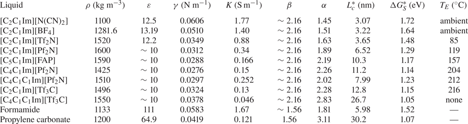
5. Conclusions
The first-principles model for the ion emission regime presented in this article captures the phenomenology observed in experiments. The model shows that ion emission can take place from the tip of a Taylor cone-like meniscus anchored on a tubular emitter. The emitted current strongly depends on the solvation energy of the ion,  ${\Delta G}_S$, and current values comparable to those measured in experiments are obtained when using typical solvation energies. The current is proportional to the potential of the emitter, and increases with the electrical conductivity and surface tension of the liquid. The model is also useful to understand the governing physics. A key result is the increase of the temperature at the tip resulting from ohmic dissipation. There is a positive feedback between ion emission and tip temperature: increasing emission increases ohmic dissipation; this increases the tip temperature, which increases the conductivity of the liquid; this increases the emission. For low values of ${\Delta G}_S$ the ion emission and the temperature are unphysically high, because at such temperatures the liquid may decompose and/or evaporate, which is not considered by the model.
We have also developed a simplified analytical model to derive scaling laws for the emitted current and the size of the emission area, as well as criteria for identifying liquids that are likely to operate in the ion emission regime. The model is based on the electrostatic solution for the ideal Taylor cone. This assumption may be inaccurate near the tip of the meniscus, but the detailed numerical solution corroborates the validity of the analytical model. In the analytical expression for the current density the emission of ions is proportional to the normal component of the outer electric field on the surface,  $E_n^o$, which drives two processes acting in series: the injection of charge on the surface by conduction from the bulk, and the evaporation of charge from the surface restricted by the energy barrier. In the tip of the Taylor cone $E_n^o$ tends to infinity, the energy barrier impeding ion evaporation is negligible, and the emission of ions is limited by the charge that bulk conduction injects on the surface. Most of the ions are emitted from this region, which has a characteristic length $L_c=({\cos \theta _T q^6 \alpha \gamma })/({8{\rm \pi} ^2{\varepsilon _0}^3{{\Delta G}_S}^4})$ and a characteristic current density $J_\omega = ({K}/{\varepsilon }) \sqrt {2\gamma \cos \theta _T/(\varepsilon _0 L_c)}$. The resulting emitted current scales as $I_c = ({\cos ^2{\theta _T}}/{8{\rm \pi} })({\alpha ^{3/2} q^9K\gamma ^2}/{{\varepsilon _0}^5\varepsilon {{\Delta G}_S}^6})$. These results show the importance of the ion solvation energy in determining the total emitted current and the size of the emission region, and the lesser but important roles played by the electrical conductivity and the surface tension. Finally, we find a criterion for an ion–liquid pair to operate in the ion emission regime, ${\Delta G}_S \lesssim ({q^{3/2} \alpha ^{1/4} \beta ^{1/2} \rho ^{1/12} \gamma ^{1/6} K^{1/6}})/{2{\rm \pi} {\varepsilon _0}^{11/12}}$. This criterion predicts well the ability of an ionic liquid for operating in ion emission regime.
The size of the emission region is near the limits of application of the continuum hypothesis. Our model could be improved by relaxing this assumption near the vertex of the meniscus, and replacing this small region with boundary conditions obtained from molecular dynamics or a similar calculation. Nonetheless, our model reproduces the main characteristics of the ion emission regime, and improves our understanding of this problem.
Funding
This work was funded by the Air Force Office of Scientific Research, award number FA9550-21-1-0200, and an Air Force Research Laboratory grant, award number F1SRQ21019M001.
Declaration of interests
The authors report no conflict of interest.
Appendix A. Definition of the orthogonal grids of regions 3 and 4
The equation sets applied in regions 3 and 4 of the domain (figure 1) are solved using finite differences along the orthogonal coordinates  $\{\xi _3,\eta _3\}$ for region 3 and $\{\xi _4,\eta _4\}$ for region 4 (see figure 14).

Figure 14. Orthogonal and surface reference frames defined near the meniscus tip.
Region 3, corresponding to the area near the tip of the meniscus, is bounded by the surface of the liquid on top and the symmetry axis on the bottom. Its geometry is well suited for applying the method defined by Srinivas & Fletcher (Reference Srinivas and Fletcher2002), where the grid is constructed by defining  $\eta _3$ ranging from the axis ( $\eta _3=0$) to the surface ( $\eta _3=1$), while $\xi _3$ is obtained by solving
 \begin{equation} \frac{{\rm d}\xi_3}{{\rm d}\eta_3}=\frac{\dfrac{\partial x}{\partial\xi_3}\dfrac{\partial x}{\partial\eta_3}+\dfrac{\partial r}{\partial\xi_3}\dfrac{\partial r}{\partial\eta_3}}{\left(\dfrac{\partial x}{\partial\xi_3}\right)^2+\left(\dfrac{\partial r}{\partial\xi_3}\right)^2} \end{equation}
from the liquid surface to the symmetry axis:  $\xi _3$ is defined along the surface of the liquid going from $\xi _3=0$ upstream to $\xi _3=1$ at the tip of the meniscus, then (A1) is integrated from $\eta _3=1$ to $\eta _3=0$ to obtain the orthogonal grid.
Region 4 encloses the first portion of the ion beam, and it often has a significant difference in radial size from start (the liquid surface) to end. The aforementioned method used for region 3 would generate a grid with significant distortion close to the symmetry axis. The orthogonal grid of region 4 is constructed from the ion trajectories, by defining the coordinate  $\xi _4$ along the characteristic lines computed by (3.26a,b).
Together with  $\{\xi _3,\eta _3\}$ and $\{\xi _4,\eta _4\}$, a third set of coordinates $\{t,n\}$ is defined along the surface of the liquid, to easily manage quantities that extend along the whole liquid surface.
We define the differential operators along the  $\{\xi _3,\eta _3\}$ and $\{\xi _4,\eta _4\}$ orthogonal grids as
 \begin{gather} \left. \begin{gathered} \frac{\partial}{\partial x}=\frac{\partial\xi}{\partial x}\frac{\partial}{\partial\xi}+\frac{\partial\eta}{\partial x}\frac{\partial}{\partial\eta},\\ \frac{\partial}{\partial r}=\frac{\partial\xi}{\partial r}\frac{\partial}{\partial\xi}+\frac{\partial\eta}{\partial r}\frac{\partial}{\partial\eta}, \end{gathered} \right\} \end{gather}
 \begin{gather} \left. \begin{gathered} \frac{\partial^2}{\partial x^2}=\frac{\partial\xi}{\partial x}^2\frac{\partial^2}{\partial\xi^2}+\frac{\partial\eta}{\partial x}^2\frac{\partial^2}{\partial\eta^2}+2\frac{\partial\xi}{\partial x}\frac{\partial\eta}{\partial x}\frac{\partial^2}{\partial\xi\partial\eta}+\frac{\partial^2\xi}{\partial x^2}\frac{\partial}{\partial\xi}+\frac{\partial^2\eta}{\partial x^2}\frac{\partial}{\partial\eta},\\ \frac{\partial^2}{\partial r^2}=\frac{\partial\xi}{\partial r}^2\frac{\partial^2}{\partial\xi^2}+\frac{\partial\eta}{\partial r}^2\frac{\partial^2}{\partial\eta^2}+2\frac{\partial\xi}{\partial r}\frac{\partial\eta}{\partial r}\frac{\partial^2}{\partial\xi\partial\eta}+\frac{\partial^2\xi}{\partial r^2}\frac{\partial}{\partial\xi}+\frac{\partial^2\eta}{\partial r^2}\frac{\partial}{\partial\eta}. \end{gathered} \right\} \end{gather}
To compute the  $\xi$ and $\eta$ differentials in these equations we must redefine them as
 \begin{gather} \left. \begin{gathered} \frac{\partial\xi}{\partial x}=\dfrac{\dfrac{\partial r}{\partial\eta}}{\dfrac{\partial x}{\partial\xi}\dfrac{\partial r}{\partial\eta}-\dfrac{\partial x}{\partial\eta}\dfrac{\partial r}{\partial\xi}} \quad \dfrac{\partial\xi}{\partial r}=\dfrac{-\dfrac{\partial x}{\partial\eta}}{\dfrac{\partial x}{\partial\xi}\dfrac{\partial r}{\partial\eta}-\dfrac{\partial x}{\partial\eta}\dfrac{\partial r}{\partial\xi}},\\ \dfrac{\partial\eta}{\partial x}=\dfrac{-\dfrac{\partial r}{\partial\xi}}{\dfrac{\partial x}{\partial\xi}\dfrac{\partial r}{\partial\eta}-\dfrac{\partial x}{\partial\eta}\dfrac{\partial r}{\partial\xi}} \quad \dfrac{\partial\eta}{\partial r}=\dfrac{\dfrac{\partial x}{\partial\xi}}{\dfrac{\partial x}{\partial\xi}\dfrac{\partial r}{\partial\eta}-\dfrac{\partial x}{\partial\eta}\dfrac{\partial r}{\partial\xi}}, \end{gathered} \right\} \end{gather}
 \begin{gather} \left. \begin{gathered} \dfrac{\partial^2\xi}{\partial x^2}=\dfrac{\begin{array}{c}\left(\dfrac{\partial^2r}{\partial\xi^2}\dfrac{\partial x}{\partial\eta}-\dfrac{\partial^2x}{\partial\xi^2}\dfrac{\partial r}{\partial\eta}\right)\dfrac{\partial r}{\partial\eta}^2+\left(\dfrac{\partial^2r}{\partial\eta^2}\dfrac{\partial x}{\partial\eta}-\dfrac{\partial^2x}{\partial\eta^2}\dfrac{\partial r}{\partial\eta}\right)\dfrac{\partial r}{\partial\xi}^2\\ +2\dfrac{\partial r}{\partial\xi}\dfrac{\partial r}{\partial\eta}\left(\dfrac{\partial^2x}{\partial\xi\partial\eta}\dfrac{\partial r}{\partial\eta}-\dfrac{\partial^2r}{\partial\xi\partial\eta}\dfrac{\partial x}{\partial\eta}\right)\end{array}}{\left(\dfrac{\partial x}{\partial\xi}\dfrac{\partial r}{\partial\eta}-\dfrac{\partial x}{\partial\eta}\dfrac{\partial r}{\partial\xi}\right)^3},\\ \dfrac{\partial^2\xi}{\partial r^2}=\dfrac{\begin{array}{c}\left(\dfrac{\partial^2r}{\partial\xi^2}\dfrac{\partial x}{\partial\eta}-\dfrac{\partial^2x}{\partial\xi^2}\dfrac{\partial r}{\partial\eta}\right)\dfrac{\partial x}{\partial\eta}^2+\left(\dfrac{\partial^2r}{\partial\eta^2}\dfrac{\partial x}{\partial\eta}-\dfrac{\partial^2x}{\partial\eta^2}\dfrac{\partial r}{\partial\eta}\right)\dfrac{\partial x}{\partial\xi}^2\\ +2\dfrac{\partial x}{\partial\xi}\dfrac{\partial x}{\partial\eta}\left(\dfrac{\partial^2x}{\partial\xi\partial\eta}\dfrac{\partial r}{\partial\eta}-\dfrac{\partial^2r}{\partial\xi\partial\eta}\dfrac{\partial x}{\partial\eta}\right)\end{array}}{\left(\dfrac{\partial x}{\partial\xi}\dfrac{\partial r}{\partial\eta}-\dfrac{\partial x}{\partial\eta}\dfrac{\partial r}{\partial\xi}\right)^3},\\ \dfrac{\partial^2\eta}{\partial x^2}=\dfrac{\begin{array}{c}\left(\dfrac{\partial^2x}{\partial\xi^2}\dfrac{\partial r}{\partial\xi}-\dfrac{\partial^2r}{\partial\xi^2}\dfrac{\partial x}{\partial\xi}\right)\dfrac{\partial r}{\partial\eta}^2+\left(\dfrac{\partial^2x}{\partial\eta^2}\dfrac{\partial r}{\partial\xi}-\dfrac{\partial^2r}{\partial\eta^2}\dfrac{\partial x}{\partial\xi}\right)\dfrac{\partial r}{\partial\xi}^2\\ +2\dfrac{\partial r}{\partial\xi}\dfrac{\partial r}{\partial\eta}\left(\dfrac{\partial^2r}{\partial\xi\partial\eta}\dfrac{\partial x}{\partial\xi}-\dfrac{\partial^2x}{\partial\xi\partial\eta}\dfrac{\partial r}{\partial\xi}\right)\end{array}}{\left(\dfrac{\partial x}{\partial\xi}\dfrac{\partial r}{\partial\eta}-\dfrac{\partial x}{\partial\eta}\dfrac{\partial r}{\partial\xi}\right)^3},\\ \dfrac{\partial^2\eta}{\partial r^2}=\dfrac{\begin{array}{c}\left(\dfrac{\partial^2x}{\partial\xi^2}\dfrac{\partial r}{\partial\xi}-\dfrac{\partial^2r}{\partial\xi^2}\dfrac{\partial x}{\partial\xi}\right)\dfrac{\partial x}{\partial\eta}^2+\left(\dfrac{\partial^2x}{\partial\eta^2}\dfrac{\partial r}{\partial\xi}-\dfrac{\partial^2r}{\partial\eta^2}\dfrac{\partial x}{\partial\xi}\right)\dfrac{\partial x}{\partial\xi}^2\\ +2\dfrac{\partial x}{\partial\xi}\dfrac{\partial x}{\partial\eta}\left(\dfrac{\partial^2r}{\partial\xi\partial\eta}\dfrac{\partial x}{\partial\xi}-\dfrac{\partial^2x}{\partial\xi\partial\eta}\dfrac{\partial r}{\partial\xi}\right)\end{array}}{\left(\dfrac{\partial x}{\partial\xi}\dfrac{\partial r}{\partial\eta}-\dfrac{\partial x}{\partial\eta}\dfrac{\partial r}{\partial\xi}\right)^3} \end{gathered} \right\} \end{gather}
so that we can compute them along the  $\xi =const$ and $\eta =const$ lines of the orthogonal grids.
For the  $\{t,n\}$ reference frame the differential operators are defined as
 \begin{gather} \left. \begin{gathered} \frac{\partial}{\partial x}=t_x\frac{\partial}{\partial t}+t_r\frac{\partial}{\partial n},\\ \frac{\partial}{\partial r}=t_r\frac{\partial}{\partial t}-t_x\frac{\partial}{\partial n}, \end{gathered} \right\} \end{gather}
 \begin{gather} \left. \begin{gathered} \frac{\partial^2}{\partial x^2}={t_x}^2\frac{\partial^2}{\partial t^2}+{t_r}^2\frac{\partial^2}{\partial n^2}+2t_xt_r\frac{\partial^2}{\partial t\partial n}+\left(t_x\frac{\partial t_x}{\partial t}+t_r\frac{\partial t_x}{\partial n}\right)\frac{\partial}{\partial t}+\left(t_x\frac{\partial t_r}{\partial t}+t_r\frac{\partial t_r}{\partial n}\right)\frac{\partial}{\partial n},\\ \frac{\partial^2}{\partial r^2}={t_r}^2\frac{\partial^2}{\partial t^2}+{t_x}^2\frac{\partial^2}{\partial n^2}-2t_xt_r\frac{\partial^2}{\partial t\partial n}+\left(t_r\frac{\partial t_r}{\partial t}-t_x\frac{\partial t_r}{\partial n}\right)\frac{\partial}{\partial t}+\left(t_x\frac{\partial t_x}{\partial n}-t_r\frac{\partial t_x}{\partial t}\right)\frac{\partial}{\partial n}, \end{gathered} \right\} \end{gather}
where  $t_x$, $t_r$ are the axial and radial components of the vector tangential to the liquid surface. We can also define a relation between the three reference frames valid on the liquid surface,
 \begin{equation} \left. \begin{gathered} \frac{\partial}{\partial t}=\left[-\sqrt{\frac{\partial\xi_3}{\partial x}^2+\frac{\partial\xi_3}{\partial r}^2}\frac{\partial}{\partial\xi_3}\right]_{\eta_3=1}=\left[\sqrt{\frac{\partial\eta_4}{\partial x}^2+\frac{\partial\eta_4}{\partial r}^2}\frac{\partial}{\partial\eta_4}\right]_{\xi_4=0},\\ \frac{\partial}{\partial n}=\left[\sqrt{\frac{\partial\eta_3}{\partial x}^2+\frac{\partial\eta_3}{\partial r}^2}\frac{\partial}{\partial\eta_3}\right]_{\eta_3=1}=\left[\sqrt{\frac{\partial\xi_4}{\partial x}^2+\frac{\partial\xi_4}{\partial r}^2}\frac{\partial}{\partial\xi_4}\right]_{\xi_4=0}. \end{gathered} \right\} \end{equation}
Due to the orthogonality of these sets of coordinates, we define a series of identities useful to simplify the equation set of the model,
 \begin{equation} \left. \begin{gathered} \frac{\partial\xi}{\partial x}\dfrac{\partial\eta}{\partial x}+\dfrac{\partial\xi}{\partial r}\dfrac{\partial\eta}{\partial r}=0,\\ \dfrac{\dfrac{\partial\xi}{\partial x}}{\sqrt{\dfrac{\partial\xi}{\partial x}^2+\dfrac{\partial\xi}{\partial r}^2}}=\dfrac{\dfrac{\partial\eta}{\partial r}}{\sqrt{\dfrac{\partial\eta}{\partial x}^2+\dfrac{\partial\eta}{\partial r}^2}},\\ \dfrac{\dfrac{\partial\xi}{\partial r}}{\sqrt{\dfrac{\partial\xi}{\partial x}^2+\dfrac{\partial\xi}{\partial r}^2}}=\dfrac{-\dfrac{\partial\eta}{\partial x}}{\sqrt{\dfrac{\partial\eta}{\partial x}^2+\dfrac{\partial\eta}{\partial r}^2}},\\ \sqrt{\dfrac{\partial\xi}{\partial x}^2+\dfrac{\partial\xi}{\partial r}^2}\sqrt{\dfrac{\partial\eta}{\partial x}^2+\dfrac{\partial\eta}{\partial r}^2}=\dfrac{\partial\xi}{\partial x}\dfrac{\partial\eta}{\partial r}-\dfrac{\partial\eta}{\partial x}\dfrac{\partial\xi}{\partial r}\\ t_x={-}n_r \quad t_r=n_x \quad t_x n_x+t_r n_r=0\\ t_x\dfrac{\partial t_x}{\partial t}={-}t_r\dfrac{\partial t_r}{\partial t} \quad t_x\dfrac{\partial t_x}{\partial n}={-}t_r\dfrac{\partial t_r}{\partial n}. \end{gathered} \right\} \end{equation}
Appendix B. Definition of the liquid surface in polar coordinates
For the optimization phase of the model, the surface of the meniscus is defined in polar coordinates as  $\varrho (\theta )$ (figure 15), to avoid numerical instabilities at the vertex of the meniscus ( $\theta =0$) and at the anchoring point with the emitter ( $\theta ={\rm \pi} /2$). In this frame of reference we define the normal and tangential vectors to the surface as
 \begin{gather} \begin{bmatrix} t_x\\ t_r \end{bmatrix}=\dfrac{1}{\sqrt{\varrho^2+{\varrho'}^2}}\begin{bmatrix} -\varrho\sin\theta+\varrho'\cos\theta\\ \varrho\cos\theta+\varrho'\sin\theta \end{bmatrix}, \end{gather}
 \begin{gather} \begin{bmatrix} n_x\\ n_r \end{bmatrix}=\dfrac{1}{\sqrt{\varrho^2+{\varrho'}^2}}\begin{bmatrix} \varrho\cos\theta+\varrho'\sin\theta\\ \varrho\sin\theta-\varrho'\cos\theta \end{bmatrix}. \end{gather}
To define the surface tension stress in polar coordinates we also require the normal vector  $\boldsymbol {n}$ in the $\{\theta,\varrho \}$ reference frame
 \begin{equation} \begin{bmatrix} n_\theta\\ n_\varrho \end{bmatrix}=\dfrac{1}{\sqrt{\varrho^2+{\varrho'}^2}}\begin{bmatrix} -\varrho'\\ \varrho \end{bmatrix} \end{equation}
from which we define the surface tension stress as
 \begin{align} \gamma\boldsymbol{\nabla}\boldsymbol{\cdot}\boldsymbol{n}&=\gamma\left[\frac{1}{\varrho^2}\frac{\partial\left(\varrho^2n_\varrho\right)}{\partial\varrho}+\frac{1}{\varrho\sin\theta}\frac{\partial\left(n_\theta\sin\theta\right)}{\partial\varrho}\right]\nonumber\\ &=\frac{\gamma}{\sqrt{\varrho^2+{\varrho'}^2}}\left(2-\frac{\varrho\varrho''-{\varrho'}^2}{\varrho^2+{\varrho'}^2}-\frac{\varrho'}{\varrho\sin\theta}\right). \end{align}
Figure 15. Polar coordinates defined for the liquid meniscus surface.


 Open access