


1. Introduction
Interactions between eddies and large-scale flows affect in important ways the properties of general circulation in the ocean and atmosphere. In this work, we attempt to elucidate key elements of these interactions in the simplest setting, by studying the evolution of a localized vortex embedded in a zonal background flow. We use the framework of a 1.5-layer quasi-geostrophic (QG) model on a  $\beta $-plane, which is derived from the rotating shallow-water equations in the limit of small Rossby number (see, for example, Zeitlin Reference Zeitlin and Zeitlin2007), leading to the well-known equation for the conservation of QG potential vorticity (PV); in plasma physics, the analogous equation is known as the Hasegawa-Mima equation (see, for example, Tur & Yanovsky Reference Tur and Yanovsky2017). Elementary analysis below shows that the quasi-geostrophic potential vorticity (QGPV) equation, as well as the rotating shallow-water equations it originates from, are non-invariant relative to Galilean transformations to a reference frame in uniform motion with respect to the original reference frame. This non-invariance is of no dynamical significance in the absence of the mean flow, but it turns out to be important and bears non-trivial consequences for interactions of eddies with such flows, even in the simplest case when the mean flow is itself uniform.
Eddy–mean-flow interactions in a rotating fluid have been a subject of extensive research efforts. For example, Vandermeirsch et al. (Reference Vandermeirsch, Carton and Morel2003a,Reference Vandermeirsch, Carton and Morelb) and Sokolovskiy et al. (Reference Sokolovskiy, Carton, Filyushkin and Yakovenko2016) examined mutual influences of a vortex and a narrow jet in the context of ocean dynamics; Vandermeirsch et al. (Reference Vandermeirsch, Carton and Morel2003a) also provide a short but informative review of earlier studies on the subject. A major focus of these studies was to clarify physical mechanisms and conditions for the vortex to cross the jet axis. Similar theoretical studies in atmospheric settings (Gilet, Plu & Riviere (Reference Gilet, Plu and Riviere2009); Oruba, Lapeyre & Riviere (Reference Oruba, Lapeyre and Riviere2012, Reference Oruba, Lapeyre and Riviere2013), among others) emphasized effects of vortex deformation by the shear flow on vortex dynamics. In a more applied work, Tamarin & Kaspi (Reference Tamarin and Kaspi2016, Reference Tamarin and Kaspi2017) proposed an explanation of the observed downstream poleward deflection of the midlatitude storm tracks which involved baroclinic self-interaction of the cyclones accompanied by diabatic heating and non-uniform background-flow advection. However, a simple and potentially important effect of Galilean non-invariance of the governing equations on the dynamics of localized vortices in such systems has thus far been largely overlooked. In the present work, we address this problem via numerical simulations of the QGPV equation describing the motion of a monopolar singular vortex (hereafter SV) embedded in a uniform zonal flow, using the algorithm developed in Kravtsov & Reznik (Reference Kravtsov and Reznik2019); hereafter KR2019.
In the latter study, the authors demonstrated that in the absence of the mean flow, the SV evolution exhibits three stages. The first – linear – stage is characterized by the formation, in the neighbourhood of the SV, of a regular dipolar field ( $\beta $-gyres), which advects the SV along the dipole axis. At the initial time, this axis is oriented along the meridian, but is quickly turned by the vortex in the direction of the SV rotation, resulting in the singular cyclone moving northwest and singular anticyclone moving southwest. The development of $\beta $-gyres was studied by many authors using analytical (Reznik Reference Reznik1992; Reznik & Dewar Reference Reznik and Dewar1994; Sutyrin & Flierl Reference Sutyrin and Flierl1994; Llewellyn Smith Reference Llewellyn Smith1997) and numerical approaches (Sutyrin et al. Reference Sutyrin, Hesthaven, Lynov and Rasmussen1994; Lam & Dritschel Reference Lam and Dritschel2001; Early, Samelson & Chelton Reference Early, Samelson and Chelton2011), as well as laboratory experiments (for example, Carnevale, Kloosterziel & van Heijst Reference Carnevale, Kloosterziel and van Heijst1991).
During the second stage, which was not described prior to KR2019, the regular field's dipolar structure disintegrates and the SV gets embedded into the  $\beta $-gyres’ lobe of the opposite polarity, forming a new dipolar singular–regular pair, which still propagates north-westward for the case of the singular cyclone and south-westward for the singular anticyclone. In this stage, the radiation of the Rossby waves by the SV and self-interactions within the regular field play an important role, making the underlying dynamics fundamentally nonlinear; hence, it seems reasonable to call this stage a nonlinear stage.
Finally, at the third, frictional stage, the effects of horizontal viscosity come into play; during this stage, the SV's motion is near uniform and the regular field stays nearly constant in the reference frame associated with the SV. While KR2019 documented the occurrence of these three stages of SV evolution, physical mechanisms governing the dynamics during each stage and transitions between these stages remained unclear. A more in-depth examination of these mechanisms constitutes the second major goal of the present study, with the emphasis on the first two stages – quasi-linear and nonlinear; the horizontal hyperviscosity in the present high-resolution model is taken to be minimal and the frictional stage does not occur, at least throughout the duration of numerical experiments.
The remainder of the paper is organized as follows. In § 2, we formulate the governing equations and show that, due to their Galilean non-invariance, even the simplest, zonally uniform background flow substantially modifies the dynamics of localized vortices superimposed on this flow, with or without  $\beta $-effect. The rest of the work is mainly devoted to the examination of an isolated SV embedded in a uniform zonal flow. In § 3, we derive the system of equations describing the evolution of such a SV (some invariants of motion associated with these equations are given in appendix A), briefly describe the numerical formulation and outline the numerical experiments, which effectively extend those in KR2019 to a wider range of model parameters. Sections 4 and 5 present the results of these experiments. In § 6, we detail the mechanisms governing the evolution of a localized vortex. Finally, § 7 contains the discussion of our main findings and their geophysical applications.
2. Localized vortices in background zonal flow
2.1. Problem formulation
The QGPV equation for the 1.5-layer fluid on a  $\beta $-plane is
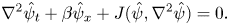
 \begin{equation}{({\nabla ^2}\hat{\psi } - {a^2}\hat{\psi })_t} + \beta {\hat{\psi }_x} + J(\hat{\psi },{\nabla ^2}\hat{\psi }) = 0.\end{equation}
 Here  $\hat{\psi } = \hat{\psi }(x,y,t)$ is the streamfunction, $a = R_d^{ - 1}$ is the inverse Rossby radius ${R_d}$, the parameter $\beta $ is the y-derivative of the Coriolis parameter at the reference latitude, the subscripts t and x denote partial differentiation with respect to time t and x-coordinate, respectively, ${\nabla ^2}$ is the Laplacian and J is the Jacobian.
Now consider a localized vortex-like disturbance in a purely zonal background flow with the streamfunction  $\bar{\psi }(\kern0.4pt y)$. At the initial time, the streamfunction $\hat{\psi }$ is
 \begin{equation}{\hat{\psi }_I} = \bar{\psi }(\kern0.4pt y) + {\tilde{\psi }_I}(x,y);\quad {\tilde{\psi }_I}(x,y) \to 0,\;r \to \infty;\end{equation}
hereafter, the subscript I denotes the initial field, so  ${\tilde{\psi }_I}(x,y)$ is our initial localized vortex. The solution of the problem (2.1), (2.2) can be written as follows:
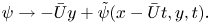
 \begin{equation}\hat{\psi } = \bar{\psi }(\kern0.4pt y) + \tilde{\psi }(x,y,t);\quad \tilde{\psi } \to 0,\;r \to \infty;\quad \tilde{\psi }{|_{t = 0}} = {\tilde{\psi }_I},\end{equation}
while (2.1) reduces to the following equation for the localized vortex streamfunction  $\tilde{\psi }$
 \begin{equation}{({\nabla ^2}\tilde{\psi } - {a^2}\tilde{\psi })_t} + \bar{\beta }{\tilde{\psi }_x} + J(\bar{\psi } + \tilde{\psi },{\nabla ^2}\tilde{\psi } - {a^2}\tilde{\psi }) = 0,\end{equation}
where
 \begin{equation}\bar{\beta } = \bar{\beta }(\kern0.4pt y) = \beta + {\bar{Q}_y};\quad \bar{Q} = {\partial _{yy}}\bar{\psi } - {a^2}\bar{\psi }.\end{equation}
 Note that, hereafter, we will use the notation  $Q = {\nabla ^2}\psi - {a^2}\psi $ for the relative potential vorticity, as in (2.5) for the background flow or $\tilde{Q} = {\nabla ^2}\tilde{\psi } - {a^2}\tilde{\psi }$ – for the PV associated with the localized vortex disturbance. The relative potential vorticity is a sum of the vertical component of vorticity ${\nabla ^2}\psi $ and the vertical vortex-tube stretching $- {a^2}\psi $. In (2.5), we have also used an alternative notation for the partial y-derivative ${\partial _y}$, with the second derivative denoted as ${\partial _{yy}}$ and so forth.
2.2. Uniform zonal flow
For the simplest case of a uniform zonal background flow with zero shear we have
 \begin{equation}\bar{\psi }(\kern0.4pt y) ={-} \bar{U}y;\quad {\partial _y}\bar{Q} ={-} {a^2}{\partial _y}\bar{\psi } = {a^2}\bar{U},\end{equation}
where  $\bar{U} = \textrm{const}\textrm{.}$ is the background-flow velocity. The effective $\beta $-parameter here is
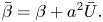 \begin{equation}\bar{\beta } = \beta + {a^2}\bar{U}.\end{equation}
In the coordinate system associated with the background flow, that is,
 \begin{equation}x^{\prime} = x - \bar{U}t;\quad y^{\prime} = y;\quad t^{\prime} = t,\end{equation}
equations (2.4) and (2.3) take the form (the primes are omitted)
 \begin{equation}{({\nabla ^2}\tilde{\psi } - {a^2}\tilde{\psi })_t} + \bar{\beta }{\tilde{\psi }_x} + J(\tilde{\psi },{\nabla ^2}\tilde{\psi }) = 0;\quad \tilde{\psi }{|_{t = 0}} = {\tilde{\psi }_I}.\end{equation}
 From (2.7) and (2.9) it follows that, in the coordinate system (2.8a–c), the vortex moves in the same way as in the absence of the background zonal flow, but with a modified  $\beta $-parameter equal to $\bar{\beta }$. The problem (2.9) has been actively studied in the past (see, for example, Reznik Reference Reznik1992; Reznik & Dewar Reference Reznik and Dewar1994; Sutyrin & Flierl Reference Sutyrin and Flierl1994; Sutyrin et al. Reference Sutyrin, Hesthaven, Lynov and Rasmussen1994; Reznik, Grimshaw & Benilov Reference Reznik, Grimshaw and Benilov2000; Lam & Dritschel Reference Lam and Dritschel2001; Early et al. Reference Early, Samelson and Chelton2011; KR2019). Based on these studies, one can provide a qualitative description of the vortex motion relative to the background zonal flow as a function of
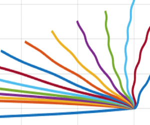
  $\bar{U}$ (see figure 1 for the case of a cyclone). When $\bar{\beta } \gt 0$, a cyclone moves north-westward, with the eastward mean flow ( $\bar{U} \gt 0$) enhancing the $\beta $-effect and making the vortex move faster to the north and west relative to the mean flow than for the case $\bar{U} = 0$. The stronger the background flow $\bar{U} \gt 0$ is, the larger the effective $\beta $-parameter $\bar{\beta } = \beta + {a^2}\bar{U}$ and the faster the vortex motion relative to the background flow are. Note that, in general, the vortex velocities depend on time and are not necessarily parallel for different $\bar{U}$, as shown in our schematic figure 1 $(a \ne 0)$.

Figure 1. A cartoon of the vortex velocity vector (red arrows) relative to a uniform zonal background flow depending on the flow's velocity  $\bar{U}$. (a) The general case with $a \ne 0,\beta \ne 0$; (b) the case where $a \ne 0,\beta = 0$; (c) the barotropic case, in which $a = 0,\beta \ne 0$. In the latter case, the relative velocity of the vortex is independent of $\bar{U}$.
For the westward background flow  $\bar{U} \lt 0$, the $\beta $-drift of the vortex and its advection by the mean flow are of the same sign, so, for small-to-moderate $|\bar{U}|$, the vortex outruns the mean flow, but when $\bar{U}$ reaches the maximum (negative) velocity of Rossby waves $- \beta R_d^2$, the effective $\beta $-parameter becomes $\bar{\beta } = 0$, and the vortex stops moving relative to the mean flow. Further increase of $|\bar{U}|$ leads to $\bar{\beta } \lt 0$ and the vortex's motion against the mean flow, with a cyclone moving south-eastward and anticyclone north-eastward.
From (2.7), it follows that similar considerations also apply in the absence of the  $\beta $-effect, when $\beta = 0$. In this case, the original equation (2.1) does not, by itself, contain preferential directions, but a zonal background flow brings in anisotropy and induces its own $\beta $-effect characterized by the effective $\beta $-parameter $\bar{\beta } = {a^2}\bar{U}$, which is proportional to the background-flow velocity $\bar{U}$. For any non-zero value of $\bar{U}$, the vortex will move in the same direction as the mean flow but will lag behind the mean flow (figure 1). In addition, the vortex will also have a velocity component normal to the mean flow: in particular, a cyclone will move to the left and anticyclone – to the right of the mean flow. In summary, even in the absence of the $\beta $-effect, a uniform background flow does not simply advect a vortex, but makes the vortex move along a complex curved trajectory with respect to the background flow.
Generation of the  $\beta $-effect by a uniform background flow is due to the vortex-tube stretching associated with the term $- {a^2}\psi $ in the relative PV Q. In the barotropic case where a = 0, (2.1) takes the form
 \begin{equation}{\nabla ^2}{\hat{\psi }_t} + \beta {\hat{\psi }_x} + J(\hat{\psi },{\nabla ^2}\hat{\psi }) = 0.\end{equation}
Equation (2.10) possesses Galilean invariance, that is, the invariance with respect to the transformation
 \begin{equation}\psi \to - \bar{U}y + \tilde{\psi }(x - \bar{U}t,y,t).\end{equation}
Accordingly, in this case, there is no generation of the additional  $\beta $-effect, and the vortex motion relative to the background flow does not depend on $\bar{U}$ (see figure 1). On the other hand, if $a \ne 0$, the solution of (2.1) is not invariant with respect to the transformation (2.11), and the relative vorticity $\bar{Q}$ associated with the uniform background flow $\bar{\psi } ={-} \bar{U}y$ is non-zero – $\bar{Q} = {a^2}\bar{U}y$ – resulting in the generation of the background-flow-induced $\beta $-effect. The above arguments demonstrate that the Galilean non-invariance of (2.1) stems from the fact that this equation describes the motion of a fluid in a non-inertial rotating coordinate system in the presence of the vertical vortex-tube stretching. It is readily shown that the original rotating shallow-water equations, from which (2.1) is derived, are also non-invariant to the Galilean transformations.
Thus, the presence of a uniform background flow modifies strongly even the f-plane dynamics by permitting Rossby waves which, in turn, determine the evolution of localized monopoles. On a  $\beta $-plane, the effective $\beta $-parameter $\bar{\beta }$ is the sum (2.7) of the planetary and mean-flow-induced parts, which brings about an even richer spectrum of possible flow dynamics. Generation of an additional $\beta $-effect by a homogeneous rectilinear zonal flow in model (2.1) has been known for a long time; for example, Pedlosky (Reference Pedlosky1979) showed that the effective $\beta $-parameter (2.7) enters the dispersion relation for the Rossby waves in such a flow. However, the physical reason behind this generation, namely the Galilean non-invariance of the rotating shallow-water model and of (2.1), as well as its basic effects on the eddy–mean-flow interactions were not considered previously to the best of our knowledge.
Finally, we note here that the combination of rotation and vertical vortex-tube stretching is a necessary but not sufficient condition for the Galilean non-invariance. For example, the equations describing the motion of a stratified fluid in a domain vertically confined between two parallel rigid lids do possess the Galilean invariance. In particular, in a commonly used two-layer model, in which both layers have finite depths (see, for example, Pedlosky Reference Pedlosky1979), the stretching is proportional to the difference  ${\psi _1} - {\psi _2}$ between the upper- and lower-layer streamfunctions, so adding a uniform barotropic flow does not result in changes of the effective $\beta $-parameter. The same is valid for the so-called $1{\textstyle{3 \over 4}}$-layer model (Ingersoll & Cuong Reference Ingersoll and Cuong1981; Flierl, Morrison & Swaminathan Reference Flierl, Morrison and Swaminathan2019) – the two-layer model with an infinitely deep but active lower layer. The Galilean non-invariance discussed here only takes place in a layer (stratified or homogeneous) bounded by free surfaces (from above and/or below), which separate this layer from the quiescent ambient fluid.
2.3. Estimates of vortex's zonal speed
Previous analytical and numerical results (see, for example, Reznik Reference Reznik1992; Reznik & Dewar Reference Reznik and Dewar1994; Sutyrin & Flierl Reference Sutyrin and Flierl1994; Sutyrin et al. Reference Sutyrin, Hesthaven, Lynov and Rasmussen1994; Lam & Dritschel Reference Lam and Dritschel2001; Early et al. Reference Early, Samelson and Chelton2011) combined with the arguments of § 2.2 allow one to estimate the vortex's zonal velocity U (in the absolute reference frame) depending on the background-flow velocity  $\bar{U}$. In particular, from this previous work, it is known that in the absence of the mean flow (that is, for $\bar{U} = 0$), the vortex moves westward with the velocity not exceeding the maximum (westward) velocity of the Rossby waves $- \beta R_d^2$, viz.
 \begin{equation}{-}\beta R_d^2 \lt U \lt 0.\end{equation}
For the zonal background flow such that  $- \beta R_d^2 \lt \bar{U}$ (which includes all eastward and weak-to-moderate westward flows), the effective $\beta $-parameter $\bar{\beta } \gt 0$; see (2.7). Hence, from (2.12) it follows that in the reference frame associated with the mean zonal flow, the relative zonal velocity of the vortex lies in the range $- \bar{\beta }R_d^2 \lt U \lt 0$. Combining this expression with (2.7) leads to the following estimate for the zonal velocity of the vortex in the absolute reference frame [compare with (2.12)]
 \begin{equation}{-}\beta R_d^2 \lt U \lt \bar{U}.\end{equation}
For the strong westward mean flows with
 \begin{equation}\bar{U} \lt - \beta R_d^2,\end{equation}
the effective  $\beta $-parameter $\bar{\beta }$ becomes negative, and the vortex moves eastward in the reference frame associated with the background flow; in this reference frame, the relative zonal velocity of the vortex is within the interval $(0, - \bar{\beta }R_d^2)$ [compare with (2.12)]. In the absolute reference frame, we therefore have
 \begin{equation}\bar{U} \lt U \lt - \beta R_d^2.\end{equation}
In the remainder of the paper, we will use numerical experiments to study, in detail, the motion and dynamics of singular monopoles in the presence of a uniform background zonal flow.
3. Singular monopole in background zonal flow
3.1. Problem formulation
To explore the consequences of the Galilean non-invariance of the governing equations described above, we will utilize the numerical model of interaction between localized singular vortices and a regular flow developed in KR2019. In this system, the localized initial disturbance  ${\tilde{\psi }_I}(x,y)$ in (2.2) is the Bessel SV
 \begin{equation}{\tilde{\psi }_I} ={-} \frac{A}{{2{\rm \pi} }}{K_0}[p|\boldsymbol{r} - {\boldsymbol{r}_{0I}}|],\end{equation}
where A is the constant intensity of the vortex,  ${L_v} = {p^{ - 1}}$ is its spatial scale, $\boldsymbol{r} = (x,y)$ is a coordinate vector and ${\boldsymbol{r}_{0I}}$ is the initial position of the SV. Without loss of generality, we assume that $A \gt 0$, which corresponds to (3.1) representing a singular cyclone. Accordingly, $\tilde{\psi }$ in (2.3) is given by
 \begin{equation}\tilde{\psi } = \psi + {\psi _s},\quad {\psi _s} ={-} \frac{A}{{2{\rm \pi} }}{K_0}[p|\boldsymbol{r} - {\boldsymbol{r}_0}(t)|],\end{equation}
and the equation for the regular-flow streamfunction  $\psi $ obtained from (2.4) and (3.2) is (Reznik Reference Reznik1992)
 \begin{equation}\begin{array}{ccccc} & {Q_t} + J({\psi _s},Q) + \bar{\beta }{\partial _x}{\psi _s} + ({p^2} - {a^2})J(\bar{\psi } + \psi + Uy - Vx,{\psi _s})\\ & \quad + \bar{\beta }{\partial _x}\psi + J(\bar{\psi } + \psi ,Q) ={-} K{\nabla ^6}\psi ,\quad Q = {\nabla ^2}\psi - {a^2}\psi , \end{array}\end{equation}
where we added, on the right-hand side, the hyperviscosity term  $- K{\nabla ^6}\psi $ required for numerical stability (KR2019). Equations (3.3) are supplemented by those for the SV velocity $(U,V)$ and the initial condition on $\psi $
 \begin{equation}U = {\dot{x}_0} ={-} {\partial _y}(\psi + \bar{\psi }){|_{\boldsymbol{r} = {\boldsymbol{r}_0}}},\quad V = {\dot{y}_0} = {\partial _x}\psi {|_{\boldsymbol{r} = {\boldsymbol{r}_0}}},\quad \psi {|_{t = 0}} = 0.\end{equation}
To ensure that our numerical model provides a faithful approximation of the continuous equations, we will monitor the integrals of energy E and enstrophy L, as well as the conservation of PV at the centre of the SV (Reznik Reference Reznik1992; Reznik & Kizner Reference Reznik and Kizner2007; KR2019); see appendix A.
3.2. Model parameters and numerical experiments
In this study, we examine the simplest case of the SV embedded in a uniform zonal flow with velocity  $\bar{U}$ (and the corresponding streamfunction $\bar{\psi } ={-} \bar{U}y$) by analysing numerical solutions of the system (3.2)–(3.4a–c). These equations were discretized on an equally spaced regular grid in an x-periodic channel of length ${L_x}$ and width ${L_y}$ using the second-order accuracy central differences in space subject to the no-flow and free-slip conditions on zonal boundaries ( ${\psi _x} = {\psi _y} = {\psi _{yyyy}} = 0$), the fourth-order Arakawa scheme for advection (Arakawa Reference Arakawa1966) and the leapfrog time integration scheme, as well as mass and momentum constraints (McWilliams Reference McWilliams1977). To suppress the spurious numerical mode of the leapfrog scheme, we average the variables carried by its two time levels every 100 time steps. We made sure that the geometrical parameters ${L_x}$ and ${L_y}$ are large enough so that the presence of y-boundaries and x-cyclicity have essentially no effect on the motion of the singular vortex throughout the duration of our numerical experiments; hence, our numerical solutions effectively approximate the solutions in an unbounded domain.
Following KR2019, the analytical Bessel SV (3.1) was replaced, in our numerical formulation, by its finite-difference analogue; given the current SV location  ${\boldsymbol{r}_0}(t)$, the regular-flow velocities $U,V$ at this location, as well as the singular streamfunction ${\psi _s}(|\boldsymbol{r} - {\boldsymbol{r}_0}(t)|)$ on the model grid in the vicinity of ${\boldsymbol{r}_0}(t)$ were both computed using cubic splines (see KR2019 for further details).
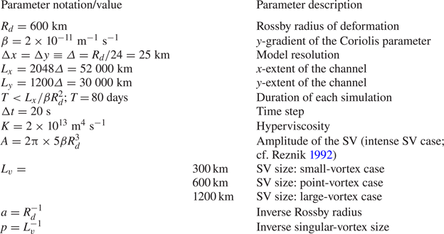
All model parameters are listed in table 1, where we also note the expressions for the domain size  $({L_x},{L_y})$, the spatial resolution $\varDelta $, the duration of each experiment T and the SV amplitude A in terms of the Rossby radius of deformation ${R_d}$ and the $\beta $-parameter. In our experiments, we chose the ‘environmental’ parameter values typical for the mid-to-high-latitude troposphere (e.g. Marshall and Molteni Reference Marshall and Molteni1993) and studied the evolution of the system on both an f-plane (with $\beta = 0$), using the $\bar{U}$ values in the range between 1 and 10 m s−1, and on a $\beta $-plane, with $\bar{U}$ in the range between –10 and 10 m s−1. All of the experiments were performed for the SVs of three different sizes ${L_v} = {p^{ - 1}}$, namely for a point vortex ( ${L_v} = {R_d};p = a$), a small vortex ( ${L_v} = {R_d}/2;p = 2a$) and a large vortex ( ${L_v} = 2{R_d};p = a/2$). In the figures below, the dimensionless streamfunction has the scale of $[\psi ] = [U][L]\;{\textrm{m}^2}\;{\textrm{s}^{-1}}$, where we used the velocity scale of $[U] = 10\;\textrm{m}\;{\textrm{s}^{-1}}$ and the length scale of $[L] = 25\;\textrm{km}$.
Table 1. Model parameters.
The results obtained below can also be interpreted in an oceanographic context by choosing the Rossby scale to be approximately ten times smaller than in the atmosphere, that is, by setting  ${R_d} = 60\;\textrm{km}$; the mean-flow velocities $\bar{U}$ should be scaled accordingly as $\beta R_d^2$, leading to values of the order of one hundredth of the corresponding atmospheric value. The appropriate grid size in this case thus becomes $\varDelta = {R_d}/24 = 2.5\;\textrm{km}$ and analogous adjustments are needed for the parameters $({L_x},{L_y})$, T and A (see table 1).
4. Point-vortex results: the case  $\beta = 0$

In this section, we will concentrate on the point vortex ( ${L_v} = {R_d};p = a$) and consider first its evolution on an f-plane ( $\beta = 0$). The point-vortex experiments on a $\beta $-plane will be analysed in § 5; the results for the small and large SVs are qualitatively similar to those for the point vortex and will be discussed in § 6.4.
4.1. Quasi-linear evolution in weak background flow
In the absence of the  $\beta $-effect, the mean-field parameters in (3.3) and (3.4a–c) are given by
 \begin{equation}\bar{\psi }(\kern0.4pt y) ={-} \bar{U}y;\quad \bar{\beta } = {a^2}\bar{U}.\end{equation}
 Without loss of generality, we assume that  $\bar{U} \gt 0$; also, for convenience, we will refer to the background flow as being zonal and call the direction normal to the flow meridional, despite the fact that at $\beta = 0$ equation (2.1) is isotropic. For weak-to-moderate background flows ( $\bar{U} \le 5\;\textrm{m}\;{\textrm{s}^{-1}}$), the SV evolves in an approximately linear regime (KR2019) throughout the simulation; in this regime, the regular streamfunction $\psi $ remains small and the full system (3.3), (3.4a–c) can be approximated, in the reference frame moving with the SV, by the following simplified system (see Reznik (Reference Reznik1992) and KR2019 for details):
 \begin{gather}{Q_t} + J({\psi _s},Q) + \bar{\beta }{\partial _x}{\psi _s} + ({p^2} - {a^2})J(\psi + {\dot{x}_0}y - {\dot{y}_0}x,{\psi _s}) = 0,\end{gather}
 \begin{gather}{\dot{x}_0} ={-} {\partial _y}\psi {|_{\boldsymbol{r} = 0}},\quad {\dot{y}_0} = {\partial _x}\psi {|_{\boldsymbol{r} = 0}},\quad \psi {|_{t = 0}} = 0.\end{gather}
 The problem (4.2), (4.3a–c) is linear in  $\psi $ and is easily solved analytically for the point vortex $p = a$ (Reznik Reference Reznik1992) and numerically for $p \ne a$ (KR2019); the resulting solution depends linearly on $\bar{\beta }$, hence the name of the linear regime it describes.
The solution  $\psi $ of (4.2), (4.3a–c) for the point-vortex case and $\bar{U} = 5\;\textrm{m}\;{\textrm{s}^{-1}}$ is shown in figure 2; the solutions for $p \ne a$ are qualitatively similar (not shown). The regular field $\psi $ of this solution is due to the near-field radiation of Rossby waves by the SV, which leads to the formation of a variable, in space and time, symmetric dipole (the so-called $\beta $-gyres) centred at the SV; this dipole in turn drives the SV self-propagation. The absence of the term $\bar{\beta }{\psi _x}$ in (4.2) inhibits the far-field radiation of Rossby waves. For $\bar{\beta } \gt 0$, the anticyclonic (cyclonic) $\beta $-gyre is located to the north-east (south-west) of the SV. At small times, the $\beta $-gyres dipole axis is oriented nearly along the meridian (not shown), but at later times the SV turns this axis counter-clockwise, resulting in the SV/ $\beta $-gyres system moving north-westward relative to the background flow (but still north-eastward in the absolute reference frame).

Figure 2. Evolution of the regular streamfunction  $\psi $ for the point SV in a uniform background flow on an f-plane ( $p = a,\textrm{ }\beta = 0,\textrm{ }\bar{U} = 5\;\textrm{m}\;{\textrm{s}^{-1}}$) obtained by solving, numerically, the linear equations (4.2), (4.3a–c). The contours show the solution in the reference frame attached to the SV (denoted by the black dot), with blue contours corresponding to the negative streamfunction values, orange contours corresponding to the positive values and the zero contour shown in black. The contour interval (CI) is 2, the maximum value of $\psi $ is given in the corner of each panel. The continuum of red dots shows the SV trajectory in the absolute reference frame. The size of the sub-region shown is approximately $50 \times 30{R_d}$. The full domain is approximately $85 \times 50{R_d}$ (table 1).
In the solution of the full system (3.3), (3.4a–c) (figure 3), the SV also moves north-eastward (that is, with a zonal component in the direction of the background flow), but the regular streamfunction field is more complex than in figure 2. This is due to the dispersion term  $\bar{\beta }{\psi _x}$ in (3.3), which is responsible for the far-field radiation of Rossby waves and the formation of the wave trail to the east of the SV; see Reznik (Reference Reznik2010) and KR2019 for a qualitative description of this process. The amplitude of the Rossby-wave far-field trail for the present case of a fairly weak background flow remains relatively small in comparison with the $\beta $-gyres, and the near-field $\beta $-gyre dipole persists throughout the simulation, but loses its symmetry in the full solution, with the anticyclonic lobe of the $\beta $-gyres progressively intensifying, the cyclonic lobe weakening, and the SV being gradually sucked into the former, which cannot happen in the purely linear regime described by (4.2), (4.3a–c) (compare with figure 2). Yet, these changes are not accompanied by the loss of the SV connection with the cyclonic $\beta $-gyre, as during the fully developed nonlinear stage of the SV evolution (see KR2019 and below), and the SV velocities and trajectories in the full solution remain close to those of the linear model (4.2), (4.3a–c) (figure 4). We therefore call the dynamical regime of SV evolution at small-to-moderate values of $\bar{U}$ (here $\bar{U} \le 5\;\; \textrm{m}\;{\textrm{s}^{-1}}$), that is, with a small-to-moderate $\bar{\beta }$, a quasi-linear regime.


Figure 4. Trajectories (top) and velocities (bottom) of the point SV for  $\beta = 0$ and different $\bar{U}$ (as shown in the legend of each panel): (a) trajectories in the absolute reference frame; (b) trajectories with respect to the background flow; (c) SV zonal velocity relative to the background flow as a function of time; and (d) SV meridional velocity as a function of time. The continuum of black dots in the bottom panels shows the solution of the linear problem (4.2), (4.3a–c). The SV velocities are normalized by $\bar{U}$ and the SV coordinates – by ${R_d}$.
For all values of the background-flow velocity  $\bar{U}$ considered here, the SV moves zonally in the direction of the background flow, but always lags behind this flow, with the SV zonal velocity U, which equals to $\bar{U}$ at the initial time, abruptly dropping, in the course of 1–2 days, to significantly smaller values (figure 4c). The SV relative ‘resistance’ to the mean flow is especially pronounced for weak flows (small $\bar{U}$). For example, by the end of the simulation, the SV zonal velocity U in the absolute reference frame for the cases $\bar{U} = 1$ and $\bar{U} = 3\;\; \textrm{m}\;{\textrm{s}^{-1}}$ amounts to only slightly over $0.1\bar{U}$ (figure 4c). The SV meridional velocity V for these weak background-flow cases first increases and then starts to decrease, ending up with the values of approximately $0.06- 0.08\bar{U}$ by the end of the simulation (figure 4d). The approximate self-similarity of the $U(t)$ and $V(t)$ curves for weak-to-moderate values of the background flow, and their proximity to the solutions of the linear model (4.2), (4.3a–c) in figures 4(c) and 4(d), respectively, is due to the latter solution's scaling linearly with $\bar{\beta }$ and, therefore, with $\bar{U}$, as readily follows from (4.2), (4.3a–c).
To summarize, the  $\beta $-effect induced by the background flow slows down the motion of the SV; without this factor, the SV would simply be ‘frozen’ in the background flow, as in the barotropic case (2.10).
4.2. Development of a nonlinear regime at large $\bar{U}$

The background-flow-induced  $\beta $-effect increases with $\bar{U}$, and the evolution of the SV becomes more complex: a relatively short quasi-linear stage gives way to the nonlinear stage, in which the dispersion term $\bar{\beta }{\psi _x}$ and the self-interactions within regular field $J(\bar{\psi } + \psi ,Q)$ in (3.3) become important. A typical example of such a behaviour is the case $\bar{U} = 10\;\; \textrm{m}\;{\textrm{s}^{-1}}$. Initially, the SV evolves in a quasi-linear regime, as seen from the plots of SV velocity in figure 4(c,d); the normalized velocities for the case $\bar{U} = 10\;\textrm{m}\;{\textrm{s}^{-1}}$ essentially coincide with the linear solution up to $t = 5$ days and stay relatively close to it up to $t = 15$ days. After this quasi-linear stage, at $t \gt 15$ days, the character of the SV evolution changes drastically. In particular, both components of the SV velocity, instead of continuing monotonic trends as in the linear solution, exhibit oscillatory behaviour (figure 4c,d). This behaviour in the zonal SV velocity is combined with a slow trend corresponding to an overall decrease of the relative $|U|$ (figure 4c), so that the SV tends to catch up with the mean flow at large times. The meridional component of SV velocity $|V|$ (figure 4d), after a quick growth and a subsequent more gradual decay during the quasi-linear stage, starts to quickly increase again, and ends up oscillating around the mean level of about $0.2\bar{U}$, which corresponds to a fairly strong northward drift of the SV. Note that the average propagation speeds of the SV grow nonlinearly with the increase of $\bar{U}$ from 5 to 10 m s−1: this doubling of $\bar{U}$ (and, hence, $\bar{\beta }$) results in a more than trifold increase in the distance travelled by the SV (compare the trajectories in figure 4a); this is yet another reason to refer to this stage of the SV evolution as the nonlinear regime.
The onset of the nonlinear regime is also apparent in the behaviour of the regular flow at  $\bar{U} = 10\;\; \textrm{m}\;{\textrm{s}^{-1}}$ (figure 5). Here again, for the initial times up to 15 days, the evolution approximately follows the quasi-linear regime shown in figures 2 and 3: the regular field $\psi $ consists mainly of the $\beta $-gyres dipole in the vicinity of the SV and a relatively weak trail of Rossby waves to the east of SV, which does not significantly affect the SV motion. However, the intensity of the anticyclonic $\beta $-gyre and the Rossby-wave far field at $\bar{U} = 10\;\textrm{m}\;{\textrm{s}^{-1}}$ both grow much faster than at $\bar{U} = 5\;\textrm{m}\;{\textrm{s}^{-1}}$ (compare figures 3 and 5). This growth is accompanied by a faster and deeper penetration of the SV into the anticyclonic $\beta $-gyre, so that at large times the SV ends up close to the centre of the latter gyre (figure 6). This $\beta $-gyre and the SV itself form a vortex pair which drifts north-westward relative to the background flow. As the SV gets sucked in the anticyclonic $\beta $-gyre, this gyre becomes more compact and nearly circular in shape and intensifies rapidly; by the end of the simulation, its intensity exceeds that of the $\bar{U} = 5\;\textrm{m}\;{\textrm{s}^{-1}}$ case by a factor of 2.5 (compare figures 3 and 5 for $t = 75$ days). On the other hand, the intensity of the cyclonic $\beta $-gyre stops increasing after the period of initial growth and, with time, turns out to be almost an order of magnitude weaker than the intensity of its anticyclonic counterpart. Even before that, the cyclonic $\beta $-gyre essentially loses its connection with the SV (figure 5). The transition from the $\beta $-gyre advection regime to the vortex-pair regime is the first major distinction between the quasi-linear and nonlinear stages of the SV evolution (KR2019).
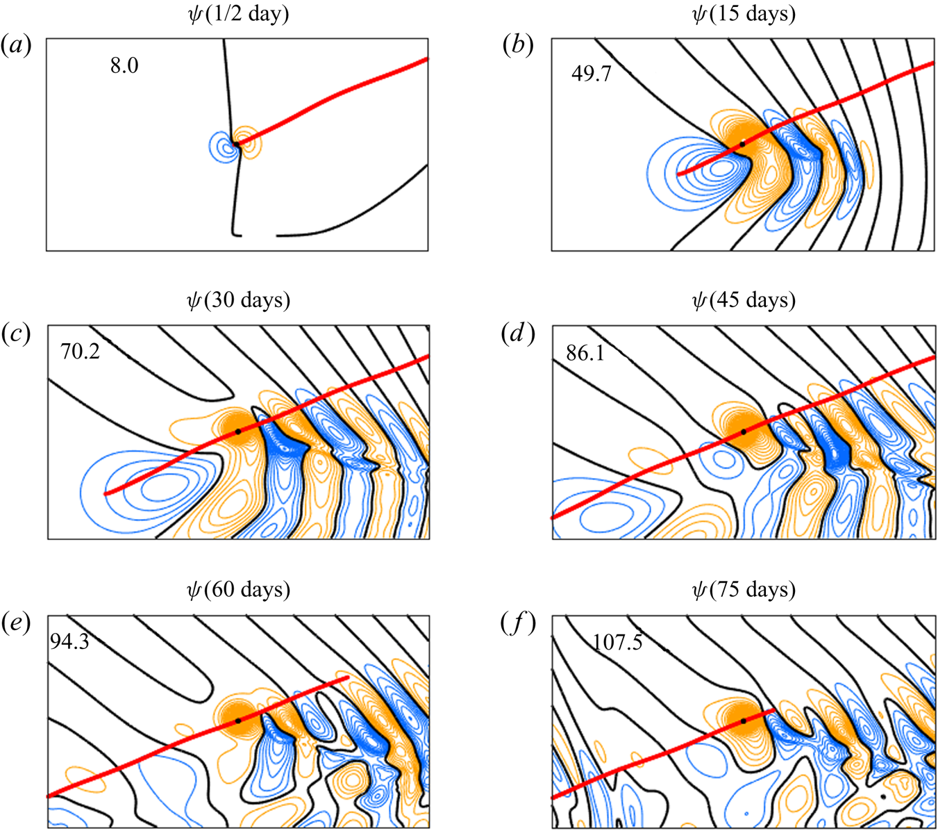
Figure 5. The same as in figure 3, but for  $\bar{U} = 10\;\textrm{m}\;{\textrm{s}^{-1}}$.
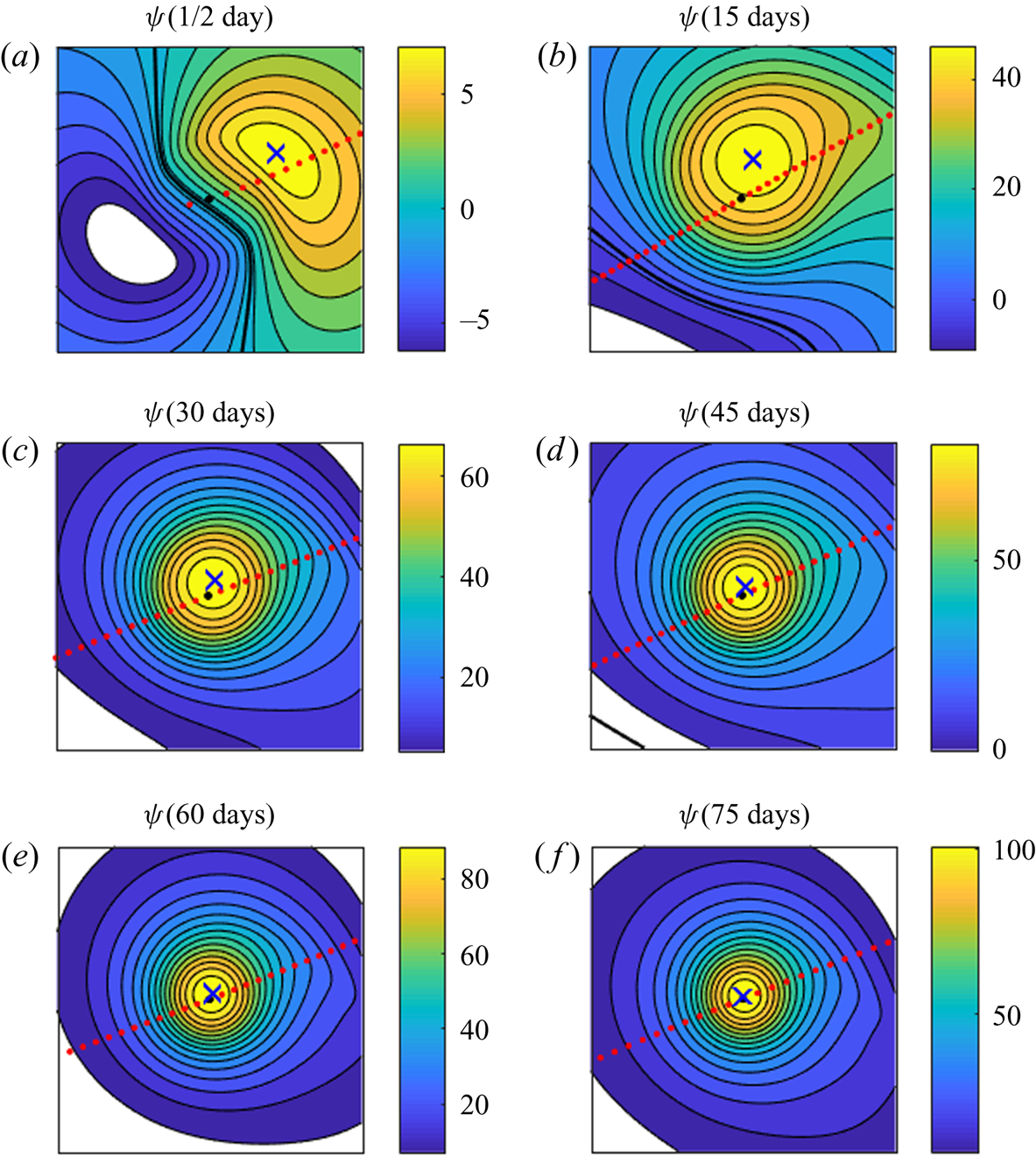
Figure 6. The merger of the point SV cyclone with the anticyclonic  $\beta $-gyre. Black contours and colour shading in each panel show the regular streamfunction at different times (see panel captions). The black dot denotes the SV position, the x-symbol marks the maximum of the regular streamfunction, which defines the centre of the anticyclonic $\beta $-gyre, red dots outline the portion of the SV trajectory in the absolute reference frame that fits into the sub-region shown. The latter sub-region has the size of approximately $4 \times 4{R_d}$.
The second major difference between the two regimes is that the Rossby-wave trail radiated by the SV, which tags along with the SV in the quasi-linear regime (see, for example, the  $t = 15$ frames in figures 3 and 5), starts to interact with the SV in the nonlinear regime (figure 5, $t \ge 15$ days), leading to oscillations in the SV propagation velocity in figure 4(c,d). Indeed, a straightforward analysis shows that the number of maxima in the SV velocity graphs coincides with the number of the Rossby-wave crests the SV passes through along its path.
5. Point-vortex results: the case $\beta \ne 0$

We saw in § 4 that on an f-plane the SV always propagates in the direction of the background flow, albeit with a smaller zonal velocity due to the flow-induced  $\beta $-effect. This is, in general, not the case for $\beta \ne 0$, where the SV can move against the zonal flow. Furthermore, with $\beta \ne 0$, the SV evolution depends on the direction of the background flow, since the effective $\beta $-parameter is given by (2.7): $\bar{\beta } = \beta + {a^2}\bar{U}$. An eastward background flow with $\bar{U} \gt 0$ always enhances the $\beta $-effect compared to the case with $\bar{U} = 0$, while a westward flow enhances the $\beta $-effect only when
 \begin{equation}\bar{U} \lt - 2\beta /{a^2},\end{equation}
and weakens the  $\beta $-effect otherwise, that is, for
 \begin{equation}{-}2\beta /{a^2} \lt \bar{U} \lt 0.\end{equation}
These statements are illustrated in figure 7. Consider first the range of negative  $\bar{U}$ from $- 5$ to $- 1\;\textrm{m}\;{\textrm{s}^{-1}}$, for which the background flow is slower than the maximum (negative) Rossby-wave velocity $- \beta R_d^2$; since $- \beta /{a^2} \lt \bar{U} \lt 0$, (5.2) is also valid, and the effective $\beta $-parameter $\bar{\beta } = \beta + {a^2}\bar{U}$ is positive and decreases with increasing $|\bar{U}|$. This means that stronger westward background flows correspond to weaker meridional displacements and meridional velocities of the SV, as clearly seen in figures 7(a) and 7(c), respectively, for weak-to-moderate westward flows with $|\bar{U}|\le 5\;\textrm{m}\;{\textrm{s}^{-1}}$. For such flows, the SV zonal velocity satisfies $- \beta R_d^2 \lt U \lt \bar{U}$ (figure 7b), so the SV outruns the westward mean flow, but is still slower than the Rossby waves. At $- 5 \le \bar{U} \le - 3\;\textrm{m}\;{\textrm{s}^{-1}}$, $\bar{\beta }$ is sufficiently small and the SV evolves in a quasi-linear regime, as seen from figure 8, in which the relative SV velocities for these cases follow the linear solution (black curves here and in figure 4c,d). Accordingly, the evolution of the regular streamfunction $\psi $ (not shown) is similar to that in figure 2.
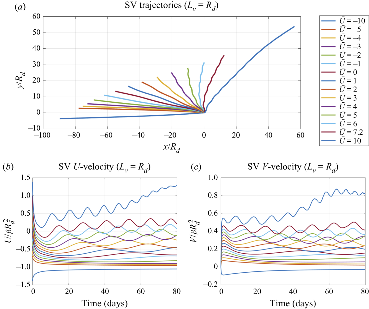
Figure 7. The point SV trajectories and velocity components in the absolute reference frame for different values of  $\bar{U}$ (see the legend); $\beta \gt 0$. The SV velocities are normalized by $\beta R_d^2$ and the SV coordinates by ${R_d}$.
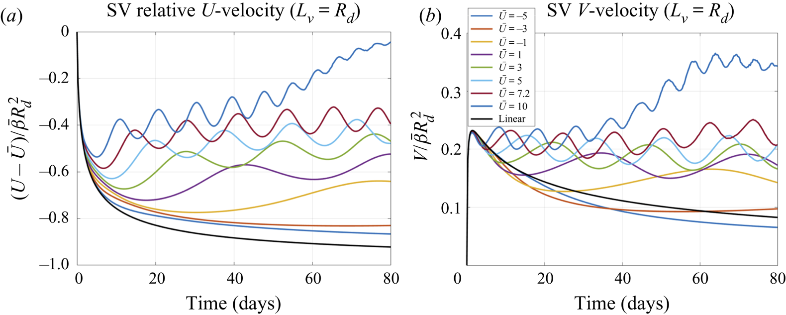
Figure 8. The same as in figure 7(b,c), but for the relative SV velocities normalized by  $\bar{\beta }R_d^2$. Black curves show the solution of the linear problem (4.2), (4.3a–c).
Consider now a moderate positive  $\bar{U}$ (eastward flow) from $1$ to $6\;\textrm{m}\;{\textrm{s}^{-1}}$, in which the SV moves in the north-westward direction opposite to the direction of the mean flow (figure 7a). For $\bar{U} \gt - 3\;\textrm{m}\;{\textrm{s}^{-1}}$, $\bar{\beta }$ becomes large enough to induce the nonlinear stage at which the normalized relative velocities for different cases diverge (figure 8). During this stage, the SV zonal velocity U oscillates about a gradually increasing mean level, so that the difference between U and $\bar{U}$ decreases with time, but the SV still continues to move to the west relative to the flow (that is, against the eastward mean flow) (figures 7 and 8). The meridional SV velocity also oscillates, but about an approximately constant mean level, leading to a fairly monotonic SV displacement to the north. The SV trajectories strongly depend on the background-flow velocity $\bar{U}$: the larger $\bar{U}$ is, the larger the SV meridional displacement and the smaller the SV zonal displacement are (figure 7a).
In particular, the ratio of the meridional to zonal SV displacement by the end of the simulation monotonically increases from about 0.04 at  $\bar{U} ={-} 5\;\textrm{m}\;{\textrm{s}^{-1}}$ to 0.25 at $\bar{U} = 0\;\textrm{m}\;{\textrm{s}^{-1}}$ to 2.7 at $\bar{U} = 5\;\textrm{m}\;{\textrm{s}^{-1}}$. We can conclude that moderate eastward flows inhibit the SV's zonal displacement and enhance its meridional displacement. Conversely, moderate westward flows ‘encourage’ the SV's zonal displacement and weaken its meridional displacement.
We have considered thus far moderate background flows, for which, in the absolute reference frame, the SV propagates north-westward and its zonal speed is bounded from below by the maximum (negative) Rossby-wave velocity  $- \beta R_d^2$ (here $- 7.2\;\textrm{m}\;{\textrm{s}^{-1}}$) (see figure 7) and does not exceed the background-flow velocity $\bar{U}$, consistent with (2.13). Let us discuss now the SV behaviour at larger values of $|\bar{U}|$. For westward flows with $\bar{U} \lt 0$, the parameter $\bar{\beta }$ reaches zero at $\bar{U} ={-} \beta R_d^2$, at which point the SV propagates westward with the mean flow and has no meridional displacement. Further decrease in $\bar{U}$ leads to $\bar{\beta }$ becoming negative and the singular cyclone moving to the south and to the east with respect to the background flow. In the absolute reference frame, the SV zonal motion satisfies (2.15): $\bar{U} \lt U \lt - \beta R_d^2$, so the SV, once again, ‘resists’ the background-flow advection. The corresponding results for the case $\bar{U} ={-} 10\;\textrm{m}\;{\textrm{s}^{-1}}$ are shown in figure 7 for the SV trajectory and velocity components and in figure 9 for the evolution of the regular field $\psi $. Due to the smallness of $\bar{\beta } \lt 0$, the SV evolves here in the quasi-linear regime. Note that the evolution of $\psi $ here is visually very different from that in the linear regime with $\bar{\beta } \gt 0$ in figure 2: in particular, the $\beta $-gyres switch locations and Rossby waves propagate to the east relative to the background flow.
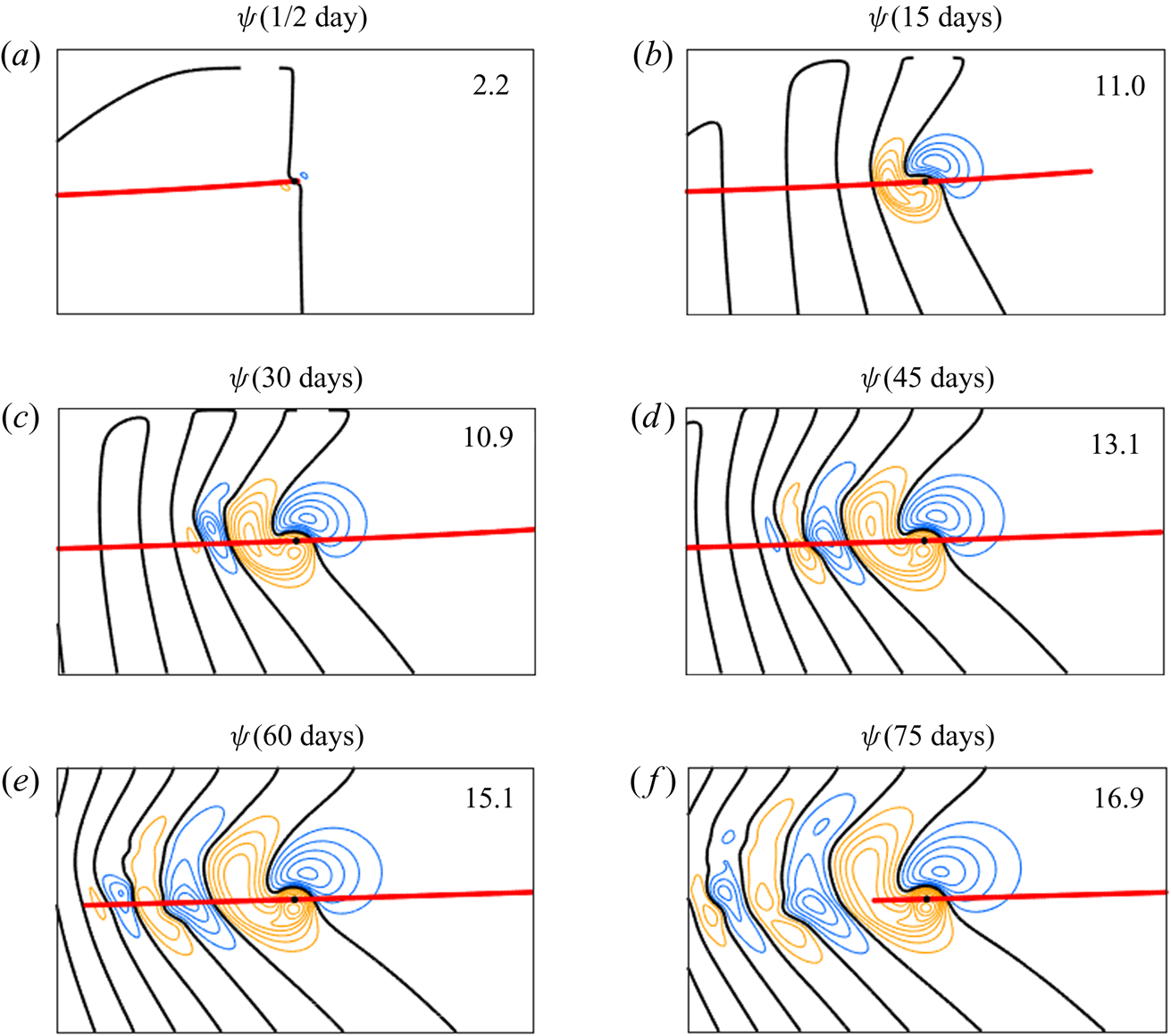
Figure 9. The same as in figure 3, but for  $\beta \gt 0$ and $\bar{U} ={-} 10\;\textrm{m}\;{\textrm{s}^{-1}}$.
For  $\bar{U} \gt 0$, the parameter $\bar{\beta }$ increases with the mean-flow speed, which leads to the shortening of the quasi-linear stage of the SV evolution, and shorter periods of the nonlinear-stage velocity oscillations (figures 7 and 8). For small and moderate values of $0 \lt \bar{U} \le 4\;\textrm{m}\;{\textrm{s}^{-1}}$ the SV zonal velocity U in the absolute reference frame quickly becomes negative during the quasi-linear stage and stays negative during the entirety of simulation (figure 7b). As $\bar{U}$ increases, the initial drop in U decreases, and U further rebounds during the nonlinear stage to become positive toward the end of the simulation (see the cases $\bar{U} = 6$ and $\bar{U} = 7.2\;\textrm{m}\;{\textrm{s}^{-1}}$ in figure 7b). For the case $\bar{U} = 10\;\textrm{m}\;{\textrm{s}^{-1}}$ the SV zonal velocity stays positive (eastward) throughout the entire simulation, approaching $\bar{U}$ toward the end of the simulation (figure 7b). In other words, the SV does get carried along by a sufficiently strong background zonal flow, but still lags behind this flow, yet with a progressively smaller lag as the time evolves. The SV meridional velocity V also increases with $\bar{U}$ (and, hence, $\bar{\beta }$; see figure 7c), leading to comparable meridional and zonal displacements of the SV at large $\bar{U}$ (see, for example, the SV trajectory for the case $\bar{U} = 10\;\textrm{m}\;{\textrm{s}^{-1}}$ in figure 7a).
6. Key elements of the SV evolution
6.1. Similarity theory
In the above discussion, we have been considering the SV of a fixed amplitude A in the background of zonal flows with different  $\bar{U}$. To study the joint effect of these two factors, it is convenient to use the similarity theory. For the case of a point vortex, the solution to the problem (3.2)–(3.4a–c) with $\bar{\psi }(\kern0.4pt y) ={-} \bar{U}y$ depends on three dimensional parameters $A,{R_d}$ and $\bar{\beta }$, from which one can form the single dimensionless parameter
 \begin{equation}\alpha = 2{\rm \pi} \bar{\beta }R_d^3/A,\end{equation}
which governs the properties of this solution. The parameter  $\alpha $ represents the scale ratio of the term $J(\psi ,Q + \bar{\beta }y)$ (advection of the regular PV by the regular flow) to the term $J({\psi _s},Q + \bar{\beta }y)$ (advection of the regular PV by the SV) in (3.3) (Reznik Reference Reznik1992). The smaller $\alpha $ is, the longer the term $\bar{\beta }{\partial _x}\psi + J(\psi ,Q)$ in (3.3) stays small relative to the other terms, and the longer the quasi-linear stage of the SV evolution is, and vice versa. According to the pi theorem (Sedov Reference Sedov1993), the SV velocities can be written as
 \begin{equation}(U,V) = \frac{A}{{{R_d}}}[{F_U}(\alpha ,\bar{t}),{F_V}(\alpha ,\bar{t})],\quad \bar{t} = \frac{A}{{R_d^2}}t,\end{equation}
where  ${F_U},{F_V}$ are some functions of $\alpha $ and $\bar{t}$. Note that there exist other, equivalent forms, of (6.2), but the particular form above is most convenient for the interpretation of our numerical experiments, which utilized the SV of a fixed amplitude A (table 1).
Our numerical experiments demonstrate that for small values of  $\alpha $ and in the quasi-linear regime, the function ${F_U}(\alpha ,\bar{t})$ monotonically decreases and the function ${F_V}(\alpha ,\bar{t})$ first increases sharply and then monotonically decreases with increasing $\bar{t}$ (see figure 4(c,d) for the cases $\bar{U} = 1\;\textrm{m}\;{\textrm{s}^{-1}}$, 3 m s−1, as well as for the linear solution; see also figure 8 for the case $\bar{U} ={-} 5\;\textrm{m}\;{\textrm{s}^{-1}}$). With increasing $\alpha $, a monotonic decay of SV velocities in time gives way to oscillations, starting at the times ${T_{{U_{min}}}} = {T_{{U_{min}}}}(\alpha )$ and ${T_{{V_{min}}}} = {T_{{V_{min}}}}(\alpha )$ corresponding to the timing of the first minimum of zonal and meridional SV velocities ${U_{min}} = {U_{min}}(\alpha )$ and ${V_{min}} = {V_{min}}(\alpha )$, respectively. The relative velocities $U(t)$, $V(t)$ normalized by ${U_{min}}$ and ${V_{min}}$ and plotted against a scaled time $t/{T_{{U_{min}}}}$(figure 10; compare with figure 8) are close to one another for different experiments, despite very different durations of these experiments in the units of the scaled time. One can hypothesize then, that at different values of $\alpha $ the SVs behave in a qualitatively similar way: during the time interval $[0,{T_{{U_{min}}}}]$, the SV evolves in the quasi-linear regime and then, for $t \gt {T_{{U_{min}}}}$, the nonlinear regime takes place. Hereafter, we will use a simpler notation ${T_{min}}$ for ${T_{{U_{min}}}}$.
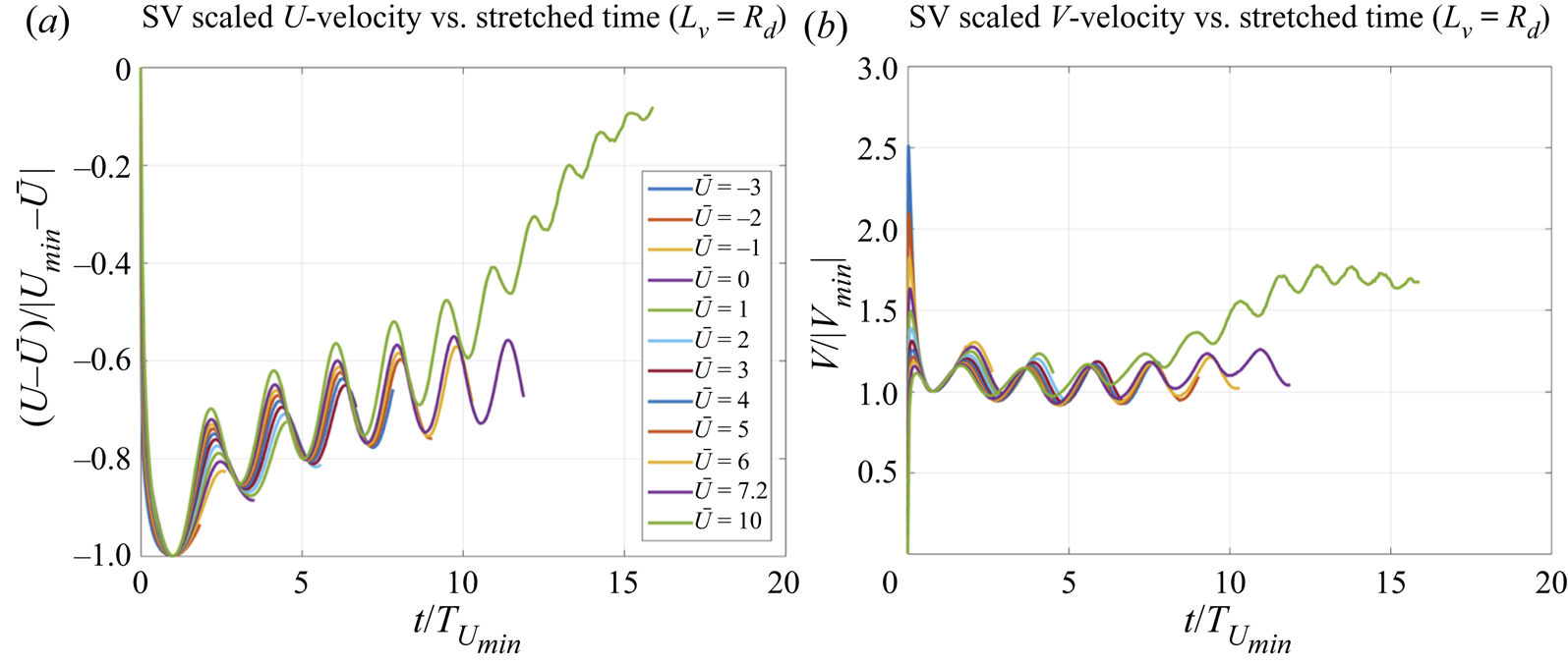
Figure 10. The dependence of scaled (relative) velocities of the SV on the stretched time (see text for details).
We can write the parameters  ${T_{min}},{U_{min}}$ as
 \begin{equation}{U_{min}} = \bar{\beta }R_d^2G(\alpha ),\quad {T_{min}} = \frac{{R_d^2}}{A}H(\alpha ),\end{equation}
where the functions  $G(\alpha ),H(\alpha )$ can be estimated from our numerical experiments. In figure 11, these functions correspond to the parameter $\bar{a} = {(p{R_d})^{ - 1}} = 1$ and are approximately equal to
 \begin{equation}G ={-} \exp( - \gamma \alpha ),\quad H = 7.63{\alpha ^{ - \mu }},\end{equation}
where  $\gamma \approx 1.37$ and $\mu \approx 1.85$. From (6.4a,b), (6.3a,b) and (6.1), it follows that the duration of the quasi-linear stage ${T_{min}}$ rapidly decreases with increasing $\bar{U}$ at a constant SV intensity A, or with decreasing A at a constant $\bar{U}$, consistent with the graphs of the SV velocities at large $\bar{U}$ in figures 4, 7 and 8. For the experiments with small and moderate values of $\bar{U}$ (see figure 4(c,d) for the cases $\bar{U} = 1\;\textrm{m}\;{\textrm{s}^{-1}}$, 3 m s−1 and figure 8 for the cases $\bar{U} ={-} 5\;\textrm{m}\;{\textrm{s}^{-1}}$, $\bar{U} ={-} 3\;\textrm{m}\;{\textrm{s}^{-1}}$), the duration of the experiment turns out to be comparable with or less than ${T_{min}}$; for example, at $\beta = 0,\bar{U} = 3\;\textrm{m}\;{\textrm{s}^{-1}}$ we estimate, from (6.4a,b), (6.3a,b) and (6.1), ${T_{min}} \approx 145$ days.
Figure 11. The dependence of (a) the first minimum of the SV zonal velocity  ${U_{min}}$ and (b) its timing ${T_{min}}$ on $\alpha = 2{\rm \pi} \bar{\beta }R_d^3/A$. The dimensionless vortex size is denoted by $\bar{a} = {(\kern0.02em p{R_d})^{ - 1}}$, the time scale $\tilde{T} = R_d^2/A$. In the legend here $\tilde{\alpha } = 2{\rm \pi} \bar{\beta }{p^{ - 3}}/A$.
In the same way, it is easy to show that the magnitude of the minimum of the SV zonal velocity  $|{U_{min}}|$ decreases with A at a fixed $\bar{U}$. In discussing the dependence of ${U_{min}}$ on $\bar{U}$, it is convenient to work with the minimum value of U in the absolute reference frame $U_{min}^{abs}$ equal to
 \begin{equation}U_{min}^{abs} = {U_{min}} + \bar{U}.\end{equation}
Using (6.5), (6.4a,b), (6.3a,b) and (2.7), we have
 \begin{equation}U_{min}^{abs} = \bar{U}(1 - {e^{ - \gamma \alpha }}) - \beta R_d^2{e^{ - \gamma \alpha }},\end{equation}
from which we can find
 \begin{equation}\frac{{\partial U_{min}^{abs}}}{{\partial \bar{U}}} = 1 - (1 - \gamma \alpha ){e^{ - \gamma \alpha }} \gt 0.\end{equation}
 Therefore, in the absolute reference frame, the first minimum of the SV zonal velocity increases with  $\bar{U}$ (compare with figure 7b).
This parameter dependence of  ${T_{min}},{U_{min}}$ implies that the duration of the quasi-linear stage of SV development decreases (and the mean-flow-induced zonal drift of the SV increases) not only with an increasing background-flow velocity $\bar{U}$ at a fixed SV intensity A, but also with a fixed $\bar{U}$ and decreasing A. In other words, the larger the parameter $\alpha $ is, that is, the smaller the relative intensity of the SV $A{\bar{\beta }^{ - 1}}$ (or the larger the relative $\beta $-effect $\bar{\beta }{A^{ - 1}}$) is, the weaker the SV resists to the background-flow-induced downstream drift of the vortex. As we will see below, this property plays an important role in the transition from the quasi-linear to the nonlinear regime of the SV evolution (§ 6.3).
6.2. Merger of cyclonic SV with anticyclonic $\beta $-gyre

We saw in § 4.2 that the drift of the SV into the  $\beta $-gyre of the opposite sign (an anticyclonic $\beta $-gyre for a singular cyclone) plays an important role in the SV evolution. We now show that this effect is purely linear and has to do with the radiation of the Rossby waves by the SV.
Consider a purely linear evolution of the SV on a  $\beta $-plane
 \begin{equation}{\partial _t}({\nabla ^2}\hat{\psi } - {a^2}\hat{\psi }) + \beta {\hat{\psi }_x} = 0,\quad \hat{\psi }{|_{t = 0}} = {\psi _s} ={-} \frac{A}{{2{\rm \pi} }}{K_0}(pr).\end{equation}
Looking for the solution in the form
 \begin{equation}\hat{\psi } = \psi + {\psi _s},\end{equation}
we find
 \begin{equation}{\partial _t}({\nabla ^2}\psi - {a^2}\psi ) + \beta {\psi _x} ={-} \beta {\partial _x}{\psi _s},\quad \psi {|_{t = 0}} = 0.\end{equation}
 The streamfunction  $\psi $ describes the Rossby-wave field radiated by the SV ${\psi _s}$. The numerical solution for $\psi $ (figure 12) shows that the SV quickly finds itself in the centre of the anticyclonic $\beta $-gyre and stays there for the duration of the experiment, with the intensity of this gyre rapidly increasing. In other words, the regular anticyclone generated in the neighbourhood of the singular cyclone tends to compensate the latter. In the linear problem (6.10), this is the consequence of the Rossby-wave dispersion, which would cause any localized regular initial disturbance to decay with time. For the singular initial condition in (6.8), this follows, first of all, from the energy equation, which can be obtained by multiplying the first equation in (6.10) by $\psi + {\psi _s}$ and area integrating over the entire plane; compare with the derivation of (A 4) in appendix A. The resulting equation
 \begin{equation}\int {\{ {\textstyle{1 \over 2}}} [{({\bf \nabla }\psi )^2} + {a^2}{\psi ^2}] - ({p^2} - {a^2}){\psi _s}\psi )\} \,\textrm{d}x\,\textrm{d}y - A\psi {|_{r = {r_0}}} = 0,\end{equation}
coincides with (A 4) at  $\bar{\psi } = 0,K = 0$. From our numerical results, it follows that the integral in (6.11) is positive (which is trivial in the case of the point vortex $p = a$) and grows with time, and so does $\psi {|_{\boldsymbol{r} = {\boldsymbol{r}_0}}}$, which indicates the strengthening in time of the anticyclonic $\beta $-gyre. Secondly, if we neglect in (6.10) the term $\beta {\psi _x}$, which is responsible for the Rossby-wave dispersion, multiply the resulting equation by ${\psi _s}$ and integrate over the plane, we get
 \begin{equation}A\psi {|_{\boldsymbol{r} = {\boldsymbol{r}_0}}} = 0.\end{equation}
Consequently, without the Rossby-wave dispersion, the SV would be bound to stay at the isoline  $\psi = 0$ and, thus, could not penetrate into the anticyclonic $\beta $-gyre.
These arguments, of course, only apply to the linear problem (6.10). To verify them in the full nonlinear problem, we computed the SV evolution according to (3.3), (3.4a–c), but without the term  $\bar{\beta }{\psi _x}$. In these experiments (figure not shown), the SV, indeed, does not leave the isoline $\psi = 0$ and, therefore, does not merge with the anticyclonic $\beta $-gyre. Recall that the term $\bar{\beta }{\psi _x}$ controls the Rossby-wave far field, while the near field ( $\beta $-gyres) is dominated by the dynamics involving the term $\bar{\beta }{\partial _x}{\psi _s}$ in (3.3).
6.3. Transition from quasi-linear to nonlinear regime
The drift of the SV toward the centre of an intensifying anticyclonic  $\beta $-gyre is equivalent to the formation, in the neighbourhood of the SV, of a growing compensating anticyclone ${\psi _a}$, so that the intensity of the total vortex ${\psi _s} + {\psi _a}$ gradually decreases with time (figure 13). The full field consists of the compact total vortex and the Rossby waves radiated by the SV earlier. Importantly, as the regular field grows in time, this full vortex monotonically weakens and becomes more compact. Hence, the effective relative amplitude of the vortex decreases, along with its capacity to ‘resist’ the advection by the mean flow (see the last paragraph of § 6.1). Accordingly, at some time, the regular PV advection terms $\bar{\beta }{\partial _x}\psi + J(\psi ,Q)$ in (3.3), which were small and could be neglected during the quasi-linear regime, become important, marking the beginning of the nonlinear regime.
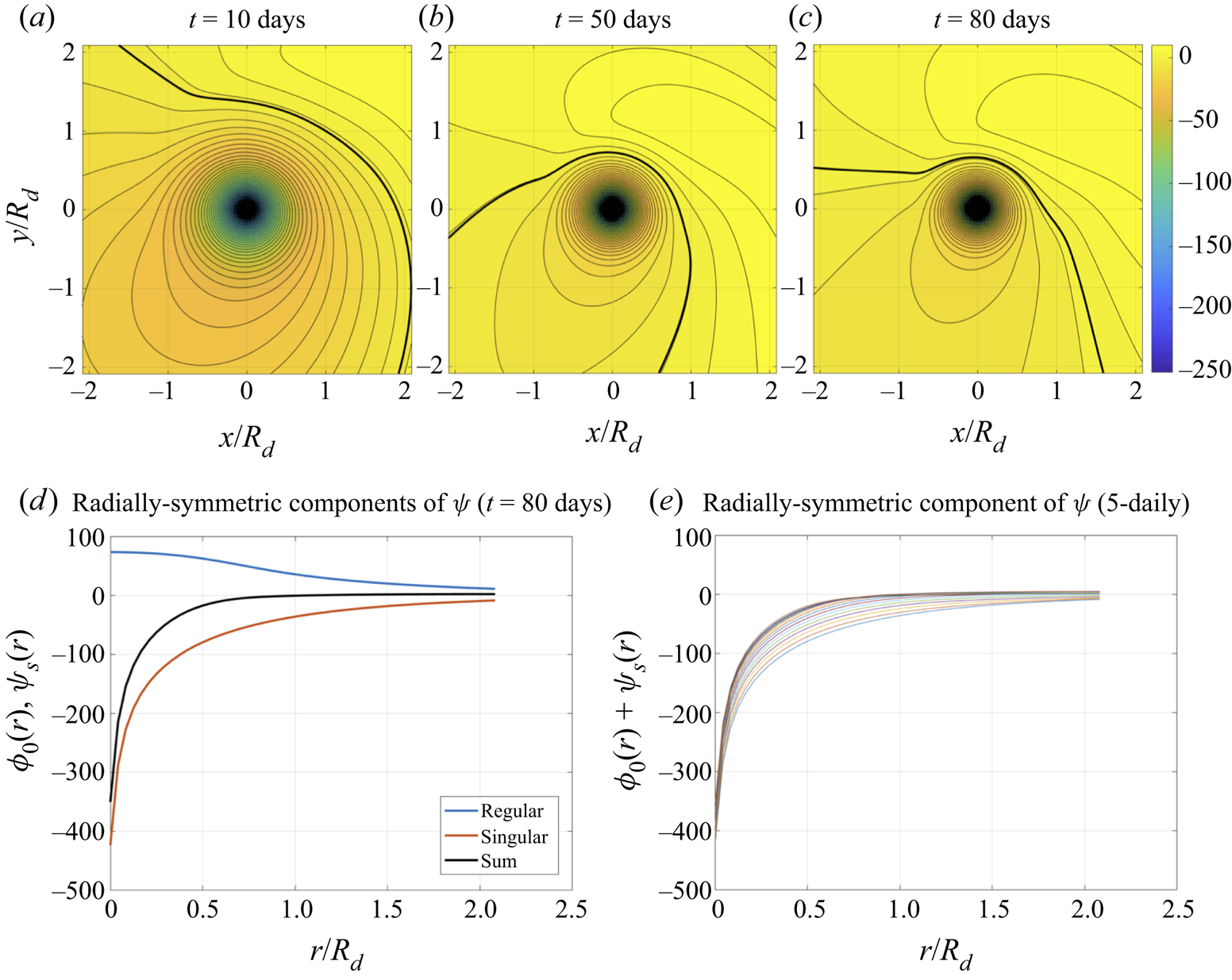
Figure 13. Evolution of the full streamfunction field  $\psi + {\psi _s}$ and its singular and regular components in the neighbourhood of the SV for the point-vortex case and $\bar{U} = 0\;\textrm{m}\;{\textrm{s}^{-1}}$. (a–c) The full streamfunction at different times (see panel captions); (d,e) The profiles of the radially symmetric streamfunction (obtained by averaging over the azimuthal angle) in the reference frame associated with the SV: (d) the profiles of the regular, singular and full streamfunction fields at t = 80 days; (e) the full streamfunction profiles shown at the 5-daily intervals (coloured curves); these profiles start from ${\psi _s}$ [red curve in (d), the bottom curve here] at t = 0 and monotonically tend to the final state at t = 80 days [black curve in (d) and the top curve here].
6.4. Sensitivity to SV size
The presentation thus far concentrated on the point-vortex case, for which  $p = a$ in (3.1). The evolution for the SV with double/half the size of the point vortex is qualitatively similar to that of the point SV. The main quantitative differences include the duration of the quasi-linear regime ${T_{min}}$, the magnitude of the first minimum of the SV zonal velocity ${U_{min}}$, as well as the amplitude of SV velocity oscillations in the nonlinear regime (figures 11 and 14). The resistance of the SV to the mean-flow advection is maximal for the large SV and minimal for the small SV, while the meridional propagation speeds for vortices of different sizes are comparable, resulting in their similar northward displacements.
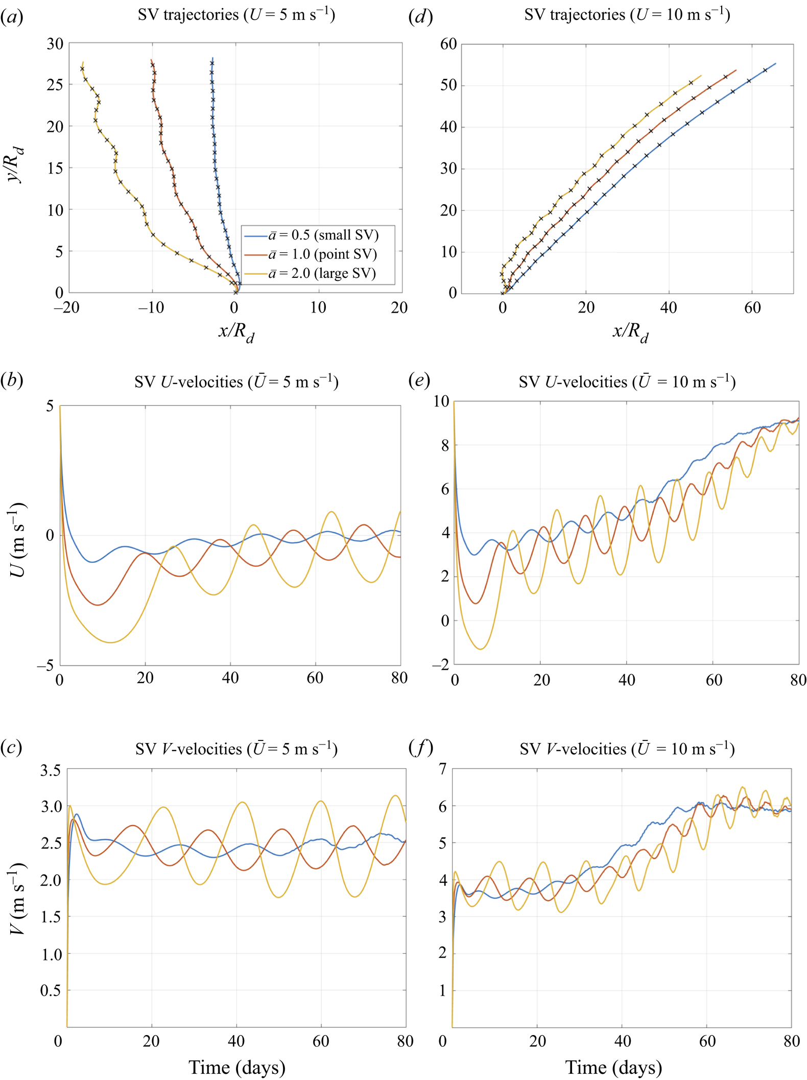
Figure 14. Trajectories and velocities of the small SV, point SV and large SV (see legend). (a–c)  $\bar{U} = 5\;\textrm{m}\;{\textrm{s}^{-1}}$; (d–f) $\bar{U} = 10\;\textrm{m}\;{\textrm{s}^{-1}}$.
7. Summary and discussion
The central result of the theory developed here is the demonstrated ability of a uniform zonal background flow to affect the motion of a vortex relative to this flow, due to the joint effect of rotation and vertical vortex-tube stretching. In the absence of at least one of these factors, this phenomenon would not be possible; for example, on a barotropic  $\beta $-plane, due to Galilean invariance of (2.10), a vortex would move relative to a uniform background flow in the same way as it would – without such a flow – in the absolute reference frame. On the other hand, the QGPV equation (2.1) for the 1.5-layer fluid considered here, as well as the shallow-water equations describing the motion of a rotating fluid, from which the QGPV equation is derived, are not invariant to the Galilean transformations owing to the effects of vortex stretching. As a result, interaction of a vortex with a uniform background flow does not reduce to a mere kinematic translation of the vortex by the mean flow, but, instead, changes the vortex dynamics. The reason lies in the fact that the background flow modifies the $\beta $-effect: in the reference frame associated with a uniform zonal background flow $\bar{U}$, the relative motion of the vortex is described by the same QGPV equation, but with the effective $\beta $-parameter $\bar{\beta } = \beta + {a^2}\bar{U}$ which includes the term proportional to $\bar{U}$; see (2.9). Therefore, the evolution of the vortex relative to the background flow is different from the $\beta $-drift in the absence of this flow.
We studied this phenomenon in the context of an isolated SV. Due to the considerations above, this problem reduces to the one for the evolution of the SV on a  $\beta $-plane with the zero background flow, but with a modified $\beta $-parameter $\bar{\beta } = \beta + {a^2}\bar{U}$. Analogous problem was addressed in KR2019, except that in that work the $\beta $-parameter was fixed, whilst here we explore a wide range of this parameter by changing $\bar{U}$. The dynamics of a point SV of intensity $A \gt 0$ (cyclone) depends on three dimensional parameters: $A,\bar{\beta }$ and the Rossby radius ${R_d} = {a^{ - 1}}$, from which one can form the single dimensionless parameter $\alpha = 2{\rm \pi} \bar{\beta }R_d^3/A$ that controls the properties of the solution. In the absence of dissipation, the SV evolution consists of two stages (or ‘regimes’). During the first, quasilinear stage, the SV motion is induced by the secondary regular dipole – the $\beta $-gyres – generated in the neighbourhood of the SV. For $\bar{U} \gt - \beta R_d^2$, the effective $\beta $-parameter is positive and the zonal (relative) SV velocity rapidly decreases from zero to a negative minimum value, while the meridional SV velocity first rapidly grows, but then also decreases to its own (positive) minimum. Decreasing (increasing) $\alpha $ amplifies (weakens) these minima and prolongs (shortens) the quasi-linear regime. In other words, the duration of the quasi-linear regime ${T_{min}}$ rapidly decreases with increasing $\bar{\beta }$ and/or decreasing A.
During the second, nonlinear stage (discovered in KR2019 and further explored in this paper), which follows the quasi-linear regime, the  $\beta $-gyres disintegrate, with the cyclonic $\beta $-gyre losing its connection with the SV and gradually disappearing, and the anticyclonic $\beta $-gyre merging with the SV to form a compact vortex pair which moves north-westward and interacts with the far-field Rossby waves radiated previously by the SV. This interaction results in oscillations in the SV velocity about an approximately constant level for its meridional component and about a slowly growing level for the zonal component, leading to a net reduction in the zonal SV motion relative to the background flow. Therefore, the SV ‘resistance’ to the mean flow weakens in the nonlinear regime.
From the SV velocities in the reference frame associated with the background flow, one can readily deduce the SV velocities in the absolute reference frame. The SV interaction with a uniform zonal flow manifests, in its purest form, on an f-plane with  $\beta = 0$. In this case, the QGPV equation does not contain preferred directions, but the inclusion of the background flow makes the problem anisotropic and creates its own, induced $\beta $-effect, with $\bar{\beta } = {a^2}\bar{U}$. In the reference frame attached to the background flow, this flow-induced $\beta $-effect makes the SV move against the flow, with the zonal speed not exceeding $|\bar{U}|$, and meridionally to the north (see figure 1). In other words, the SV resists the background advection and lags behind the background flow, but still moves, in the absolute reference frame, in the direction of, yet at an angle to the background flow, leaving the background flow on the right (figure 15a). The less the speed of the background flow and/or the more intense the SV is, the stronger the SV resists to the background advection and the more it lags behind the background flow. The SV resistance to the background flow is the strongest during the quasi-linear stage of the SV development and reduces in the nonlinear regime. The duration of the quasi-linear regime decreases with increasing $|\bar{U}|$ (see above), thus resulting in a stronger net drift of the SV in the direction of the mean flow; at the same time, the SV velocity and displacement components normal to the background flow grow as well.

Figure 15. A cartoon of the vortex velocity vector (red arrows; cf. figure 1) in the absolute reference frame for  $a \ne 0$: (a) $\beta = 0$; (b) $\beta \gt 0$.
In the general case  $\beta \ne 0$ an analogous diagram is much more complex (see figure 15b and table 2) and the SV can move both upstream and downstream. For the strong westward background flows with $\bar{U} \lt - \beta R_d^2$, the effective $\beta $-parameter is negative – $\bar{\beta } = \beta + {a^2}\bar{U} \lt 0$ – and the cyclone moves south-eastward relative to the mean flow, that is, against the latter. In the absolute reference frame, the SV drifts westward, with the velocity in between $\bar{U}$ and $- \beta R_d^2$, and southward. The SV southward displacement and its resistance to background advection both decrease as $\bar{U}$ approaches $- \beta R_d^2$; at $\bar{U} ={-} \beta R_d^2(\bar{\beta } = 0)$, the SV becomes ‘frozen’ in the background flow and moves with the mean flow in a purely zonal direction. At $\bar{U} \gt - \beta R_d^2$, the effective $\beta $-parameter becomes positive – $\bar{\beta } = \beta + {a^2}\bar{U} \gt 0$ – and increases with $\bar{U}$, leading to a progressively larger SV displacement northward.
Table 2. The range of SV velocities  $(U,V)$ in the absolute reference frame (right) depending on the background flow $\bar{U}$ (left).
The SV zonal velocity U in the absolute reference frame depends on  $\bar{U}$ in the following way: there exists a threshold velocity ${\bar{U}_0} \gt 0$ such that for $- \beta R_d^2 \lt \bar{U} \lt {\bar{U}_0}$ the SV moves westward, with U changing monotonically from $- \beta R_d^2$ to 0 as $\bar{U}$ increases from $- \beta R_d^2$ to ${\bar{U}_0}$. Thus, the eastward flow with $0 \lt \bar{U} \lt {\bar{U}_0}$ is too weak to advect the SV eastward; the vortex effectively resists the advection and drifts against the flow. At $\bar{U} = {\bar{U}_0}$, the zonal propagation of the SV is strongly inhibited, and the SV drifts practically northward. A stronger eastward flow with $\bar{U} \gt {\bar{U}_0}$ forces the SV to move eastward at all times, but with $U \lt \bar{U}$, and northward, with the SV meridional drift increasing with $\bar{U}$ and becoming comparable to the zonal drift for large $\bar{U}$. The threshold velocity ${\bar{U}_0}$ depends on the SV size and intensity: ${\bar{U}_0} = {\bar{U}_0}(A,{R_d},p) \gt 0$; for the parameters used here ${\bar{U}_0} \approx 5\text{--}7\;\textrm{m}\;{\textrm{s}^{-1}}$, with the smaller/larger value in this range corresponding to the small/large SV, and the value for the point SV in the middle.
These results have implications for the eddy–mean-flow interaction in the atmosphere and the ocean. For example, the existence of a positive threshold velocity  ${\bar{U}_0}$ points to a possibility of the predominantly meridional regimes of vortex propagation in regions of weak (or weakening) eastward zonal flows. Furthermore, according to our findings, the vortex advection by an eastward flow is necessarily accompanied by an enhanced (with respect to the reference case of no flow) poleward deflection of the vortex trajectory; the stronger the flow, the larger the deflection (compare with Orlanski Reference Orlanski1998; Tamarin and Kaspi Reference Tamarin and Kaspi2016, Reference Tamarin and Kaspi2017). By contrast, westward flows with $- \beta R_d^2 \lt \bar{U} \lt 0$ result in a decreasing poleward deflection with increasing $|\bar{U}|$, up to zero deflection at $\bar{U} ={-} \beta R_d^2$; for the even stronger westward flows with $\bar{U} \lt - \beta R_d^2$ the sign of the poleward deflection switches, with a cyclone (anticyclone) drifting southward (northward).
An anonymous reviewer of this paper kindly drew our attention to possible planetary physics implications of our results. For example, in westward jets on Jupiter the effective beta-parameter can be negative (Marcus & Shetty Reference Marcus and Shetty2011; Dowling Reference Dowling2020), similar to our case of a strong uniform westward flow. Drift rates of the Jupiter's Great Red Spot (e.g. Trigo-Rodriguez et al. Reference Trigo-Rodriguez, Sanchez-Lavega, Gomez, Lecacheux, Cola and Miyazaki2000) and of the cloud features on Neptune (Sromovsky Reference Sromovsky1991) exhibit oscillations akin to those of our singular-vortex translation speed in figures 4, 7 and 10. Of course, our model is highly idealized, and, in reality, the background zonal flow generally consists of the jets with strong velocity shears. We plan to conduct a numerical study of the singular vortices embedded in a shear background flow in the nearest future.
Acknowledgements
We are grateful to the three anonymous reviewers for their comments, which helped to improve the presentation and to C. Evans for proofreading § 1 of the paper. This work was supported by the State Assignment no. 0149-2019-0002 (development of the theoretical framework in § 2), the Russian Foundation for Basic Research, project no. 20-55-10001 (numerical formulation in § 3 and numerical experiments in § 4), as well as by the Ministry of Education and Science of the Russian Federation, grant no. 14.W03.31.0006 (numerical experiments in §§ 5 and 6).
Declaration of interests
The authors report no conflict of interest.
Appendix A. Integrals of motion
To derive the enstrophy integral, we rewrite (3.3) as
 \begin{align} & {Q_t} + J(\psi + \bar{\psi },Q + \bar{Q}) + \beta {\partial _x}(\psi + {\psi _s}) - J[{\nabla ^2}(\bar{\psi } + \psi ) - {p^2}(\bar{\psi } + \psi ),{\psi _s}]\notag\\ & \quad + ({p^2} - {a^2})J(Uy - Vx,{\psi _s}) ={-} K{\nabla ^6}\psi , \end{align}
multiply (A 1) by  ${\nabla ^2}(\bar{\psi } + \psi ) - {p^2}(\bar{\psi } + \psi )$ and take an area integral of the resulting expression over the entire plane, which gives
 \begin{equation}\dot{L} ={-} K\displaystyle\int {{\nabla ^6}\psi [{\nabla ^2}(\bar{\psi } + \psi ) - {p^2}(\bar{\psi } + \psi )]\,\textrm{d}x\,\textrm{d}y} ,\end{equation}
where
 \begin{equation}\left. {\begin{array}{* {20}{c}} {L = \displaystyle\int {[S} + ({\nabla^2}\bar{\psi } - {p^2}\bar{\psi })({\nabla^2}\psi - {p^2}\psi )]\,\textrm{d}x\,\textrm{d}y - \beta A{y_0};}\\ {S = \tfrac{1}{2}[{{({\nabla^2}\psi )}^2} + ({p^2} + {a^2}){{({\bf \nabla }\psi )}^2} + {p^2}{a^2}{\psi^2}].} \end{array}} \right\}\end{equation}
 In an analogous way, multiplying (A 1) by  $\bar{\psi } + \psi + {\psi _s}$ we obtain, after area integration, the following expression for the energy integral
 \begin{align}\left. {\begin{array}{* {20}{c}} {\dot{E} ={-} K\displaystyle\int ( \bar{\psi } + \psi + {\psi_s}){\nabla^6}\psi \,\textrm{d}x\,\textrm{d}y;}\\ \begin{array}{ccccc} &E = \displaystyle\int {\left\{ {\tfrac{1}{2}[{{({\bf \nabla }\psi )}^2} + {a^2}{\psi^2}] + {\bf \nabla }\bar{\psi }\,{\bf \nabla }\psi + {a^2}\bar{\psi }\psi - ({p^2} - {a^2}){\psi_s}(\bar{\psi } + \psi )} \right\}} \,\textrm{d}x\,\textrm{d}y\\ & \hspace{-18.5pc} - A{(\bar{\psi } + \psi )_{\boldsymbol{r} = {\boldsymbol{r}_0}}}. \end{array} \end{array}} \right\}\end{align}
Finally, the conservation of the regular component of potential vorticity at the centre of the SV is written as
 \begin{equation}Q{|_{\boldsymbol{r} = {\boldsymbol{r}_0}}} + \bar{Q}({y_0}) + \beta {y_0} = \bar{Q}({y_{0I}}) + \beta {y_{0I}}.\end{equation}


