


1 Introduction
One hypothesis for the ‘origin of life’ is that the first biomolecules were formed in undersea hydrothermal vents. In this theory, passive, anisotropic diffusion across a membrane supports the transmembrane gradients necessary for the first biochemical molecules (Martin et al. Reference Martin, Baross, Kelley and Russell2008). An experimental approach to study this theory examines simpler systems in microfluidic reactors which allows for the controlled study of the prebiotic chemistry in hydrothermal vent chimneys (Barge & White Reference Barge and White2017).
Microfluidic devices have become an important tool in modern chemistry and biomedical analytics (Nge, Rogers & Woolley Reference Nge, Rogers and Woolley2013). One application is the possibility of a ‘lab on a chip’, i.e. the miniaturization of chemical separation and analysis procedures onto a disposable device as small as a few square centimetres. The devices are typically made from etched glass or lithographically processed elastomers and the fluid flow is usually controlled mechanically by external pumps or electrically via electro-osmotic flows (Mark et al. Reference Mark, Haeberle, Roth, Von Stetten and Zengerle2010).
Recent studies have used microfluidic methods to form inorganic membranes within Y-shaped devices (Batista & Steinbock Reference Batista and Steinbock2015; Wang, Bentley & Steinbock Reference Wang, Bentley and Steinbock2017). The membranes result from chemical reactions between two different solutions that are injected separately but later merge in a long reaction channel that brings the reactants into direct contact. This merging is usually performed under low Reynolds number ( $Re$) conditions and for miscible liquids, such as aqueous solutions of NaOH, and a dissolved metal salt, such as NiCl2. At the reaction interface between these liquids, a precipitate, such as Ni(OH)2, swiftly forms a thin porous membrane (figure 1). This precipitate reaction typically involves the formation of microscopically small colloid particles and their aggregation or addition to the membrane. This phenomenon is related to so-called ‘chemical gardens’ which consist of thin cylindrical precipitate membranes separating a metal salt solution from silicate or hydroxide solutions (Makki et al. Reference Makki, Al-Humiari, Dutta and Steinbock2009; Roszol & Steinbock Reference Roszol and Steinbock2011).
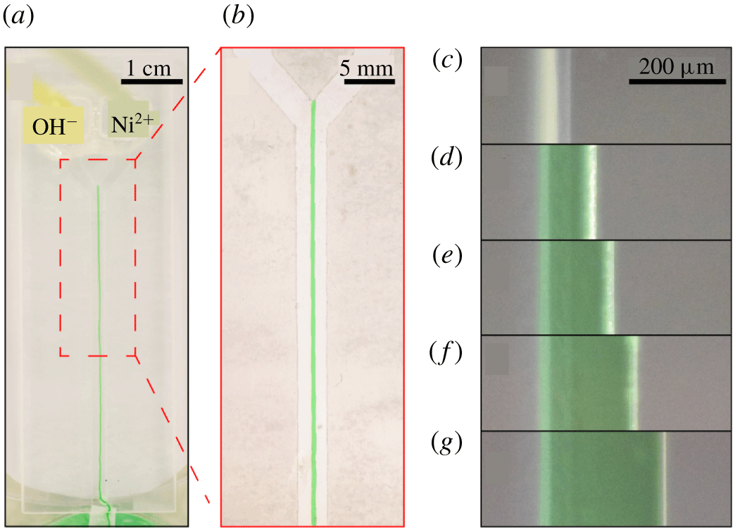
Figure 1. Inorganic precipitate membrane formed in a microfluidic channel. (a) The photograph of the resulting membrane after 2 h with 0.5 M NaOH and 0.5 M NiCl2 solutions being injected simultaneously into the microfluidic device. The mixing part of the channel is 50 mm long, 2 mm wide and approximately  $130~\unicode[STIX]{x03BC}\text{m}$ high. (b) A magnified view of a selected area from (a). (c–g) A sequence of micrographs showing the unidirectional thickening process after (c) 1 min, (d) 15 min, (e) 30 min, (f) 60 min and (g) 120 min. Scale bars correspond to (a) 1 cm, (b) 5 mm and (c)
  $200~\unicode[STIX]{x03BC}\text{m}$.
Ding et al. (Reference Ding, Batista, Steinbock, Cartwright and Cardoso2016) showed experimentally that membrane thickness increases with the square root of time, indicating diffusion-controlled growth. The membrane thickening occurs only in the direction of the metal salt solution (e.g. NiCl2) and not in the direction of the anionic precipitation partner (e.g. OH-), indicating that the membrane is more permeable to anions than cations. This phenomenon has been qualitatively explained by the charged nature of the membrane that suppresses the transmembrane transport of the positive metal ion (Batista & Steinbock Reference Batista and Steinbock2015; Wang et al. Reference Wang, Bentley and Steinbock2017).
The modelling challenges presented by this experiment involve a confluence of topics that have been studied before, namely ionic reactions (Sircar, Keener & Fogelson Reference Sircar, Keener and Fogelson2013; Yang et al. Reference Yang, Gong, Li, Eisenberg and Wang2019), precipitation (Zhang & Klapper Reference Zhang and Klapper2010; Agarwal & Peters Reference Agarwal and Peters2014), passive diffusion through a membrane (Mouritsen Reference Mouritsen2005; Cogan & Chellam Reference Cogan and Chellam2009; Ding et al. Reference Ding, Batista, Steinbock, Cartwright and Cardoso2016) and fluid–structure interaction (Vogel Reference Vogel1996; Childress, Shelley & Zhang Reference Childress, Shelley and Zhang2012; Ristroph et al. Reference Ristroph, Moore, Childress, Shelley and Zhang2012; Strychalski et al. Reference Strychalski, Copos, Lewis and Guy2015; Strychalski & Guy Reference Strychalski and Guy2016; Moore Reference Moore2017; Quaife & Moore Reference Quaife and Moore2018). The particular combination of these aspects provides the opportunity for a new model that captures them all. One key challenge is that the ‘structure’ in this problem is generated dynamically according to equations governing the chemistry. We choose to model the fluid–structure combination as a single multiphase material: one component ‘fluid’ or solvent and one component ‘structure’ or precipitate membrane. Such multiphase models have proven useful in a variety of complex-fluid applications, such as bacterial biofilms (Cogan & Keener Reference Cogan and Keener2004; Cogan & Guy Reference Cogan and Guy2010), tumour growth (Ambrosi & Preziosi Reference Ambrosi and Preziosi2002; Byrne & Preziosi Reference Byrne and Preziosi2003; Preziosi & Tosin Reference Preziosi and Tosin2009; Frieboes, Lowengrub & Cristini Reference Frieboes, Lowengrub and Cristini2010; Sorribes et al. Reference Sorribes, Moore, Byrne and Jain2019) and biological membranes (Magi & Keener Reference Magi and Keener2017); their formulation is based on averaging momentum and stresses in separated, multi-component fluids (Drew Reference Drew1983; Drew & Passman Reference Drew and Passman2006).
The multiphase framework developed here builds on previous ones (Cogan & Guy Reference Cogan and Guy2010; Zhang & Klapper Reference Zhang and Klapper2010; Leiderman & Fogelson Reference Leiderman and Fogelson2011), but with some keys differences that are guided by a combination of physical principles, model simplicity and the micro-fluidic experiments mentioned above. First, our formulation conserves the total mass of the components – solvent, dissolved species and precipitate membrane – throughout the reaction. In particular, the model accounts for changes in solute concentrations that result from the formation of new membrane and the associated exclusion of solvent volume. This effect is neglected in previous models that treat reaction chemicals as scalar fields distinct from the multiphase material, but is essential for overall mass conservation. The treatment of reaction chemicals as additional components of a multiphase material, i.e. with their own volume fractions, has been successfully modelled by many (Nunziato & Walsh Reference Nunziato and Walsh1980; Yang et al. Reference Yang, Gong, Li, Eisenberg and Wang2019) but greatly complicates the analysis, interpretation and simulation of the governing equations. Second, by making certain choices in the averaging procedure for the multicomponent stress, our formulation becomes equivalent to an incompressible Brinkman system with variable permeability.
This equivalence is important for a couple of reasons. First, it guarantees that the model reduces to the Stokes equations in the fluid limit and to Darcy’s equation in the porous-medium limit (Brinkman Reference Brinkman1949; Durlofsky & Brady Reference Durlofsky and Brady1987; Hill, Koch & Ladd Reference Hill, Koch and Ladd2001). In particular, it guarantees that when membrane is fully developed, the interface behaves as an impermeable surface without requiring any interface boundary conditions (Beavers & Joseph Reference Beavers and Joseph1967; Saffman Reference Saffman1971). As demonstrated in § 3.2, many existing multiphase models fail to exhibit this behaviour (Breward, Byrne & Lewis Reference Breward, Byrne and Lewis2003; Cogan & Keener Reference Cogan and Keener2005; Cogan & Guy Reference Cogan and Guy2010; Sorribes et al. Reference Sorribes, Moore, Byrne and Jain2019), as they were developed primarily for highly permeable systems. Second, the equivalence to Brinkman significantly simplifies the overall structure of the partial differential equation (PDE) system by eliminating certain cross-terms in the stress divergence that arise in other models.
To demonstrate that the new framework possesses the desired properties listed above, we consider a simplified system in which the incoming reactant concentrations are held fixed via chemostat (Rubinow Reference Rubinow1975). By assuming parallel flow and neglecting solute diffusion, the governing equations reduce to a planar system of ordinary differential equations (ODEs). This nonlinear system can be linearized around a fixed point and eigenvalue analysis provides an estimate for the rate at which membrane forms. Moreover, we find that the equation for the aqueous product is a second-order nonlinear ODE known as the Ricatti equation (Riccati Reference Riccati1724; Tenenbaum & Pollard Reference Tenenbaum and Pollard1985). Exact solutions to the Ricatti equation give explicit formulas for the time dependence of the chemical product and, consequently, the formation of new membrane. Once the membrane dynamics is known exactly, the flow profile can be obtained through the numerical solution of a simple boundary value problem (BVP). Visualization of the resulting flow profile allows a comparison between variants of the multiphase framework. In particular, we demonstrate that the framework developed here properly captures the transition from one-channel to two-channel flow as membrane develops.
The paper proceeds as follows: in § 2 we develop the governing equations for both the reacting chemicals and multiphase material such that the total mass is conserved. Section 3 contains analysis and results based on simplifying assumptions. These assumptions generate a reduced form for an idealized scenario which can be solved with a combination of analytic and simple numerical methods. Finally in § 4 the predictive power of the model and further applications are discussed.
2 Mathematical model
The model requires the accurate description of several aspects of the experiment, including the flow transport of the two ionic species and their reaction to form a product, the precipitation of the product out of solution and, finally, the response of the bulk fluid motion to the dynamically generated precipitate membrane. Advection–diffusion–reaction (ADR) equations are derived for the aqueous chemical concentrations, while the fluid and membrane dynamics is described by multiphase mass and momentum balance equations. In many multiphase models, either constituent can be viscous, viscoelastic, poroelastic or otherwise. Here, since the membrane adheres to the substrate, it can be treated as an immobile solid, leading to considerable simplifications.
We assume that aqueous reactants and product contribute mass, but not volume, to the fluid phase. The solvent and membrane each have their own distinct, constant mass densities, and any arbitrary control volume can be divided into solvent and membrane volume fractions. The formation of new membrane involves the precipitation of product out of solution and the sequestration of solvent. A key modelling assumption is that the volume of fluid sequestered equals the volume of the resulting membrane. As shown in § 2.2, this assumption ensures incompressibility of the phase-averaged velocity field, i.e. the so-called Darcy velocity.
We now detail the model equations. First, we derive evolution equations for the reaction of aqueous ionic species, then we list mass balances for all chemical species as well as solvent and membrane phases, and finally we describe the momentum equation for the fluid. In the end we obtain a closed, coupled PDE system governing the chemistry and physics of the system, where total mass is conserved throughout aqueous reactions and phase transitions.
2.1 Model for chemical reactions
In this section we derive equations for the chemical reactions. We follow the ‘nucleation and growth’ model of precipitation (Matsue et al. Reference Matsue, Itatani, Fang, Shimizu, Unoura and Nabika2018) and separate the reaction into two sequential parts: in the first, two reactants come together to form an aqueous product, and the second describes the aggregation of the aqueous product into a solid precipitate. While many aqueous chemical reactions do not alter the solution volume significantly, the formation of a membrane excludes fluid volume and therefore can alter the local concentration of the dissolved species. Accordingly, our model neglects the volume occupied by the aqueous species but does account for changes in species concentration that are due to the precipitated solid excluding fluid volume. This effect introduces additional terms in the aqueous reaction equations that are required for mass conservation. To our knowledge these additional terms are not accounted for in the multiphase precipitation literature that treats aqueous chemicals as scalar fields distinct from the multiphase material.
The aqueous reaction is written as a generic net ionic equation
 $$\begin{eqnarray}aA(\text{aq})+bB(\text{aq})\rightarrow cC(\text{aq}),\end{eqnarray}$$
 where  $A(\text{aq})$,
  $B(\text{aq})$ and
  $C(\text{aq})$ are chemicals in the aqueous phase and
  $a$,
$a$,  $b$ and
  $c$ are their respective stoichiometric coefficients; the precipitation reaction is written simply as
 $$\begin{eqnarray}C(\text{aq})\rightarrow C(\text{s}).\end{eqnarray}$$
As a concrete example consider the reaction described in the introduction,
 $$\begin{eqnarray}\displaystyle & \displaystyle \text{Ni}^{2+}(\text{aq})+2\text{OH}^{-}(\text{aq})\rightarrow \text{Ni(OH)}_{2}(\text{aq}), & \displaystyle\end{eqnarray}$$
 $$\begin{eqnarray}\displaystyle & \displaystyle \text{Ni(OH)}_{2}(\text{aq})\rightarrow \text{Ni(OH)}_{2}(\text{s}). & \displaystyle\end{eqnarray}$$
 Then  $A=\text{Ni}^{2+}$,
  $B=\text{OH}^{-}$ and
  $C=\text{Ni(OH)}_{2}$ and
  $a=c=1$,
  $b=2$.
The aqueous chemicals will be measured with a variable for the number of chemicals per unit solvent volume, i.e. molarity, which we will call  $\unicode[STIX]{x1D713}_{i}$ for chemical species
  $i\in \{A,B,C\}$. Reaction rates depend on a reactants’ molarity, and molarity can change due to two independent factors: either the number of molecules changes due to the aqueous reaction, or the solvent volume changes due to precipitation. Because either one can occur in a precipitation reaction, these two competing effects must be carefully considered when formulating the reaction equations.
We begin by deriving equations for how the aqueous reaction proceeds in a spatially homogeneous environment; later in § 2.2 the effects of advective and diffusive spatial fluxes will be added. Suppose the chemicals exist in some aqueous solution of fixed control volume  $V_{0}$. The chemicals undergo both the aqueous and precipitation reactions which results in fluid mass and solvent volume being converted to membrane mass and volume (see figure 2). The fluid component has mass
 $$\begin{eqnarray}{\mathcal{M}}_{f}=\left(\unicode[STIX]{x1D70C}_{s}+\sum M_{i}\unicode[STIX]{x1D713}_{i}\right)\unicode[STIX]{x1D703}_{s}V_{0},\end{eqnarray}$$
 where  $\unicode[STIX]{x1D70C}_{s}$ is the constant solvent mass density (without any reactants or products present),
  $\unicode[STIX]{x1D703}_{s}$ is the solvent volume fraction and
  $M_{i}$ is the molar mass of chemical species
  $i$. The summation represents the contribution of the chemical species to fluid mass, so that the fluid mass density is not constant. The membrane component has mass
  ${\mathcal{M}}_{m}=\unicode[STIX]{x1D70C}_{m}\unicode[STIX]{x1D703}_{m}V_{0}$ where
  $\unicode[STIX]{x1D70C}_{m}$ is the constant membrane mass density and
  $\unicode[STIX]{x1D703}_{m}$ is the membrane volume fraction. Physically, membrane mass is composed of both precipitated chemical
  $C$ and sequestered solvent mass.
The change in  $\unicode[STIX]{x1D713}_{i}$ purely due to aqueous reaction, i.e. no precipitation, can be modelled as a second-order kinetics reaction
 $$\begin{eqnarray}\dot{\unicode[STIX]{x1D713}}_{A}^{(aq)}=-ar\unicode[STIX]{x1D713}_{A}\unicode[STIX]{x1D713}_{B},\quad \dot{\unicode[STIX]{x1D713}}_{B}^{(aq)}=-br\unicode[STIX]{x1D713}_{A}\unicode[STIX]{x1D713}_{B},\quad \dot{\unicode[STIX]{x1D713}}_{C}^{(aq)}=cr\unicode[STIX]{x1D713}_{A}\unicode[STIX]{x1D713}_{B},\end{eqnarray}$$
 where the dot indicates a derivative with respect to time,  $r$ is the rate of aqueous reaction per chemical concentration and the (
 $aq$) superscript refers to the fact that (2.6) models the change in
  $\unicode[STIX]{x1D713}_{i}$ purely due to aqueous reaction, i.e. (2.1). More general power laws are sometimes used to model chemical kinetics, but here we use purely second-order kinetics for simplicity (see Chang & Goldsby Reference Chang and Goldsby2013, pp. 573–575). None of the analysis, however, depends specifically on this choice and the results could be carried forward for other kinetics.
To derive equations for the change in  $\unicode[STIX]{x1D713}_{i}$ purely due to precipitation we appeal to ideas from continuum mechanics. The concentration of ions
  $A$ in the control volume is written as
  $\unicode[STIX]{x1D713}_{A}=n_{A}/(\unicode[STIX]{x1D703}_{s}V_{0})$ where
  $n_{A}$ is the number of
  $A$ ions in
  $V_{0}$. Note that this formulation makes explicit the dependence of
  $\unicode[STIX]{x1D713}_{A}$ on both
  $n_{A}$ and
  $\unicode[STIX]{x1D703}_{s}$. Consider the change in a small increment of time
  $\unicode[STIX]{x0394}t$. Then the time-dependent variables are updated so that
 $$\begin{eqnarray}\unicode[STIX]{x1D713}_{A}+\unicode[STIX]{x0394}\unicode[STIX]{x1D713}_{A}=\frac{n_{A}}{(\unicode[STIX]{x1D703}_{s}+\unicode[STIX]{x0394}\unicode[STIX]{x1D703}_{s})V_{0}}.\end{eqnarray}$$
 Recall that  $n_{A}$ is constant during precipitation as only
  $C(\text{aq})$ precipitates. Approximating for small
  $\unicode[STIX]{x0394}\unicode[STIX]{x1D703}_{s}$ and neglecting higher-order terms gives
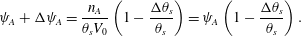 $$\begin{eqnarray}\unicode[STIX]{x1D713}_{A}+\unicode[STIX]{x0394}\unicode[STIX]{x1D713}_{A}=\frac{n_{A}}{\unicode[STIX]{x1D703}_{s}V_{0}}\left(1-\frac{\unicode[STIX]{x0394}\unicode[STIX]{x1D703}_{s}}{\unicode[STIX]{x1D703}_{s}}\right)=\unicode[STIX]{x1D713}_{A}\left(1-\frac{\unicode[STIX]{x0394}\unicode[STIX]{x1D703}_{s}}{\unicode[STIX]{x1D703}_{s}}\right).\end{eqnarray}$$
 Then, cancelling the  $\unicode[STIX]{x1D713}_{A}$, dividing both sides by
  $\unicode[STIX]{x0394}t$ and letting
  $\unicode[STIX]{x0394}t\rightarrow 0$ gives the change in
  $\unicode[STIX]{x1D713}_{A}$ purely due to precipitate reaction as
  $\dot{\unicode[STIX]{x1D713}}_{A}^{(p)}=-\unicode[STIX]{x1D713}_{A}\dot{\unicode[STIX]{x1D703}}_{s}/\unicode[STIX]{x1D703}_{s}$. By symmetry, a similar formula holds for
  $\dot{\unicode[STIX]{x1D713}}_{B}^{(p)}$. Note that both of these are essentially applications of the product rule for
  $\unicode[STIX]{x2202}_{t}(\unicode[STIX]{x1D713}_{i}\unicode[STIX]{x1D703}_{s})=0$, which physically means that the total number of ions of
  $i\in \{A,B\}$ in the control volume does not change in time due to precipitation.
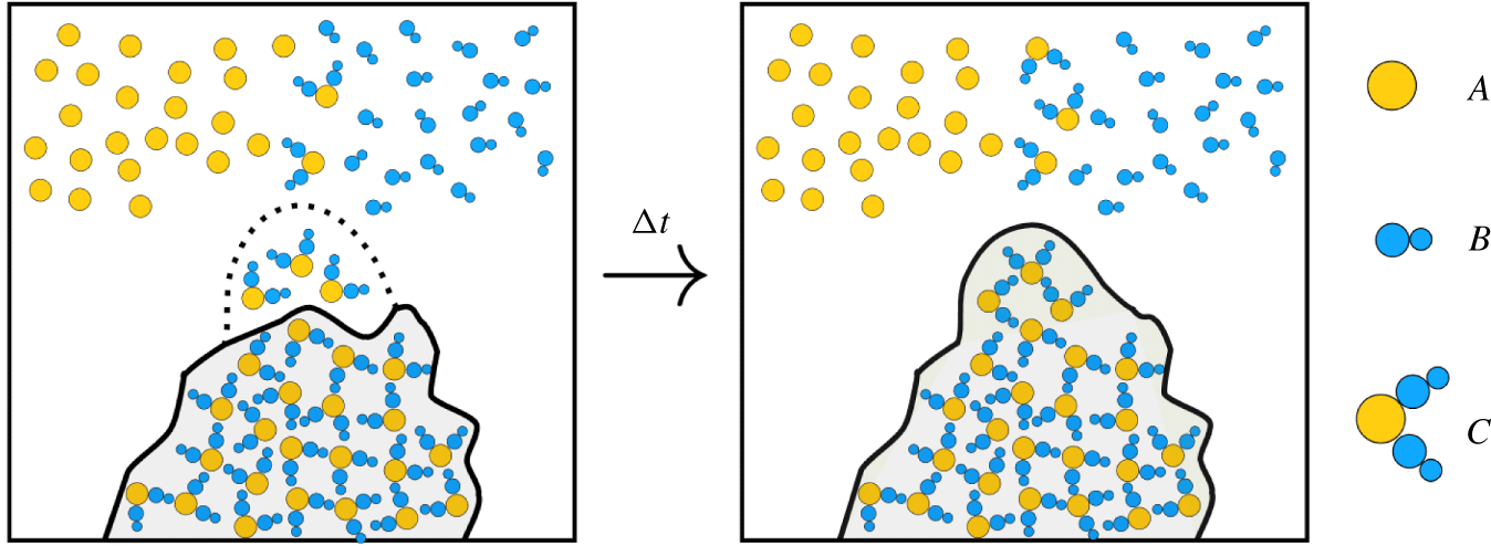
Figure 2. Schematic of precipitate reaction in control volume. Precipitation causes solution (white) to transform into membrane (shaded) after a certain concentration threshold is reached of aqueous product  $C$. Aqueous chemicals
  $A$,
$A$,  $B$ and
  $C$ are volumeless scalar fields while the solvent and membrane are treated as a multiphase material. The volume of membrane gained is exactly equal to the volume of solvent lost.
A similar procedure can be followed for  $\unicode[STIX]{x1D713}_{C}$, except now the number of aqueous chemicals
  $n_{C}$ changes as
  $C(\text{aq})$ precipitates into membrane,
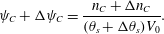 $$\begin{eqnarray}\unicode[STIX]{x1D713}_{C}+\unicode[STIX]{x0394}\unicode[STIX]{x1D713}_{C}=\frac{n_{C}+\unicode[STIX]{x0394}n_{C}}{(\unicode[STIX]{x1D703}_{s}+\unicode[STIX]{x0394}\unicode[STIX]{x1D703}_{s})V_{0}}.\end{eqnarray}$$
 Above, both  $n_{C}$ and
  $\unicode[STIX]{x1D703}_{s}$ change in time. Expanding both expressions while linearizing for small
  $\unicode[STIX]{x0394}\unicode[STIX]{x1D703}_{s}$, dividing by
  $\unicode[STIX]{x0394}t$ and taking the limit as
  $\unicode[STIX]{x0394}t\rightarrow 0$ one obtains
  $\dot{\unicode[STIX]{x1D713}}_{C}^{(p)}=-\unicode[STIX]{x1D713}_{C}\dot{\unicode[STIX]{x1D703}}_{s}/\unicode[STIX]{x1D703}_{s}+{\dot{n}}_{C}/\unicode[STIX]{x1D703}_{s}$. The first term in this expression is analogous to those obtained for reactants
  $A$ and
  $B$, and simply describes the effect on concentration when solvent volume is changing. The second term, however, is new and describes the effect on
  $\unicode[STIX]{x1D713}_{C}$ as aqueous
  $C$ molecules are converted into membrane. We write
  ${\dot{n}}_{C}=\unicode[STIX]{x1D6FC}\dot{\unicode[STIX]{x1D703}}_{s}$ where the specific value of
  $\unicode[STIX]{x1D6FC}$ will be found shortly to guarantee conservation of mass throughout the entire reaction. The expressions for the rate of change of aqueous chemical concentrations due to precipitation are thus,
 $$\begin{eqnarray}\dot{\unicode[STIX]{x1D713}}_{A}^{(p)}=-\unicode[STIX]{x1D713}_{A}\dot{\unicode[STIX]{x1D703}}_{s}/\unicode[STIX]{x1D703}_{s},\qquad \dot{\unicode[STIX]{x1D713}}_{B}^{(p)}=-\unicode[STIX]{x1D713}_{B}\dot{\unicode[STIX]{x1D703}}_{s}/\unicode[STIX]{x1D703}_{s},\qquad \dot{\unicode[STIX]{x1D713}}_{C}^{(p)}=-\unicode[STIX]{x1D713}_{C}\dot{\unicode[STIX]{x1D703}}_{s}/\unicode[STIX]{x1D703}_{s}+\unicode[STIX]{x1D6FC}\dot{\unicode[STIX]{x1D703}}_{s}/\unicode[STIX]{x1D703}_{s},\end{eqnarray}$$
 where the  $(p)$ superscript refers to the fact that (2.10) models the change in
  $\unicode[STIX]{x1D713}_{i}$ purely due to precipitation of the membrane out of solution, i.e. (2.2). Assuming that the aqueous and precipitate reactions act independently,
  $\dot{\unicode[STIX]{x1D713}}_{i}=\dot{\unicode[STIX]{x1D713}}_{i}^{(aq)}+\dot{\unicode[STIX]{x1D713}}_{i}^{(p)}$, gives
 $$\begin{eqnarray}\displaystyle & \displaystyle \dot{\unicode[STIX]{x1D713}}_{A}=-ar\unicode[STIX]{x1D713}_{A}\unicode[STIX]{x1D713}_{B}-\unicode[STIX]{x1D713}_{A}\dot{\unicode[STIX]{x1D703}}_{s}/\unicode[STIX]{x1D703}_{s}, & \displaystyle\end{eqnarray}$$
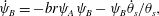 $$\begin{eqnarray}\displaystyle & \displaystyle \dot{\unicode[STIX]{x1D713}}_{B}=-br\unicode[STIX]{x1D713}_{A}\unicode[STIX]{x1D713}_{B}-\unicode[STIX]{x1D713}_{B}\dot{\unicode[STIX]{x1D703}}_{s}/\unicode[STIX]{x1D703}_{s}, & \displaystyle\end{eqnarray}$$
 $$\begin{eqnarray}\displaystyle & \displaystyle \dot{\unicode[STIX]{x1D713}}_{C}=cr\unicode[STIX]{x1D713}_{A}\unicode[STIX]{x1D713}_{B}-\unicode[STIX]{x1D713}_{C}\dot{\unicode[STIX]{x1D703}}_{s}/\unicode[STIX]{x1D703}_{s}+\unicode[STIX]{x1D6FC}\dot{\unicode[STIX]{x1D703}}_{s}/\unicode[STIX]{x1D703}_{s}. & \displaystyle\end{eqnarray}$$
 To obtain the value of  $\unicode[STIX]{x1D6FC}$ that guarantees conservation of mass, we again apply a continuum mechanics argument. The change in membrane mass after a small time step is
  $\unicode[STIX]{x0394}{\mathcal{M}}_{m}=\unicode[STIX]{x1D70C}_{m}\unicode[STIX]{x0394}\unicode[STIX]{x1D703}_{m}V_{0}$. To simplify the expression for change in fluid mass, we expand
  $\unicode[STIX]{x0394}{\mathcal{M}}_{f}$ while neglecting second-order terms to get
 $$\begin{eqnarray}\unicode[STIX]{x0394}{\mathcal{M}}_{f}=V_{0}\unicode[STIX]{x1D70C}_{s}\unicode[STIX]{x0394}\unicode[STIX]{x1D703}_{s}+V_{0}\unicode[STIX]{x1D703}_{s}\mathop{\sum }_{i}M_{i}\unicode[STIX]{x0394}\unicode[STIX]{x1D713}_{i}+V_{0}\unicode[STIX]{x0394}\unicode[STIX]{x1D703}_{s}\mathop{\sum }_{i}M_{i}\unicode[STIX]{x1D713}_{i}.\end{eqnarray}$$
 Replacing the  $\unicode[STIX]{x0394}\unicode[STIX]{x1D713}_{i}$ with their respective differential terms in (2.11) and performing some algebraic manipulation produces
 $$\begin{eqnarray}\unicode[STIX]{x0394}{\mathcal{M}}_{f}=V_{0}\unicode[STIX]{x1D70C}_{s}\unicode[STIX]{x0394}\unicode[STIX]{x1D703}_{s}+V_{0}\unicode[STIX]{x1D703}_{s}\unicode[STIX]{x1D713}_{A}\unicode[STIX]{x1D713}_{B}(cM_{c}-aM_{A}-bM_{B})+V_{0}M_{C}\unicode[STIX]{x0394}n_{C}.\end{eqnarray}$$
Conservation of mass during the aqueous reaction (2.1) implies
 $$\begin{eqnarray}aM_{A}+bM_{B}=cM_{C}.\end{eqnarray}$$
 Thus, the term in parenthesis in (2.13) vanishes. Meanwhile, conservation of mass of the entire system implies  $\unicode[STIX]{x0394}{\mathcal{M}}_{m}=-\unicode[STIX]{x0394}{\mathcal{M}}_{f}$, i.e. the mass lost by the fluid equals the mass gained by membrane. Additionally, the assumption that fluid volume is converted perfectly to membrane volume implies
  $\unicode[STIX]{x0394}\unicode[STIX]{x1D703}_{m}=-\unicode[STIX]{x0394}\unicode[STIX]{x1D703}_{s}$. Using the respective definitions of
  ${\mathcal{M}}_{i}$ and solving for
  $\unicode[STIX]{x0394}n_{C}$ gives
 $$\begin{eqnarray}\unicode[STIX]{x0394}n_{C}=\left(\frac{\unicode[STIX]{x1D70C}_{m}-\unicode[STIX]{x1D70C}_{s}}{M_{C}}\right)\unicode[STIX]{x0394}\unicode[STIX]{x1D703}_{s}.\end{eqnarray}$$
 Dividing by  $\unicode[STIX]{x0394}t$ and taking the limit
  $\unicode[STIX]{x0394}t\rightarrow 0$ gives
  ${\dot{n}}_{C}=\unicode[STIX]{x1D6FC}\dot{\unicode[STIX]{x1D703}}_{s}$ where
 $$\begin{eqnarray}\unicode[STIX]{x1D6FC}=\frac{\unicode[STIX]{x1D70C}_{m}-\unicode[STIX]{x1D70C}_{s}}{M_{C}}.\end{eqnarray}$$
 Physically, this value of  $\unicode[STIX]{x1D6FC}$ corresponds to the concentration of
  $C(\text{aq})$ that must leave the fluid phase during precipitation in order for mass to be conserved.
The reaction equations derived in this section, along with the specific  $\unicode[STIX]{x1D6FC}$ term, will be used to provide reaction terms for the chemistry mass balance equations, as described in the next section.
2.2 Mass balance equations
In experiments, the aqueous reaction occurs within the flow of a microfluidic device and therefore spatial fluxes must be considered. To describe these fluxes, consider the general conservation law for the chemical mass per unit control volume  $\unicode[STIX]{x1D719}=M_{i}\unicode[STIX]{x1D713}_{i}\unicode[STIX]{x1D703}_{s}$,
 $$\begin{eqnarray}\frac{\unicode[STIX]{x2202}\unicode[STIX]{x1D719}}{\unicode[STIX]{x2202}t}+\unicode[STIX]{x1D735}\boldsymbol{\cdot }\boldsymbol{J}=\unicode[STIX]{x1D6E4},\end{eqnarray}$$
 where  $\boldsymbol{J}$ is the flux of
  $\unicode[STIX]{x1D719}$ and
  $\unicode[STIX]{x1D6E4}$ is a transfer term for the rate that
  $\unicode[STIX]{x1D719}$ enters the system.
We choose  $\boldsymbol{J}$ to account for advection and diffusion of the chemical concentrations,
 $$\begin{eqnarray}\displaystyle & \displaystyle \frac{\unicode[STIX]{x2202}(M_{A}\unicode[STIX]{x1D713}_{A}\unicode[STIX]{x1D703}_{s})}{\unicode[STIX]{x2202}t}+\unicode[STIX]{x1D735}\boldsymbol{\cdot }(M_{A}\unicode[STIX]{x1D713}_{A}\unicode[STIX]{x1D703}_{s}\boldsymbol{v}_{s}-\unicode[STIX]{x1D705}_{A}\unicode[STIX]{x1D735}(M_{A}\unicode[STIX]{x1D713}_{A}))=\unicode[STIX]{x1D6E4}_{A}, & \displaystyle\end{eqnarray}$$
 $$\begin{eqnarray}\displaystyle & \displaystyle \frac{\unicode[STIX]{x2202}(M_{B}\unicode[STIX]{x1D713}_{B}\unicode[STIX]{x1D703}_{s})}{\unicode[STIX]{x2202}t}+\unicode[STIX]{x1D735}\boldsymbol{\cdot }(M_{B}\unicode[STIX]{x1D713}_{B}\unicode[STIX]{x1D703}_{s}\boldsymbol{v}_{s}-\unicode[STIX]{x1D705}_{B}\unicode[STIX]{x1D735}(M_{B}\unicode[STIX]{x1D713}_{B}))=\unicode[STIX]{x1D6E4}_{B}, & \displaystyle\end{eqnarray}$$
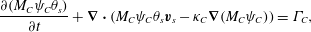 $$\begin{eqnarray}\displaystyle & \displaystyle \frac{\unicode[STIX]{x2202}(M_{C}\unicode[STIX]{x1D713}_{C}\unicode[STIX]{x1D703}_{s})}{\unicode[STIX]{x2202}t}+\unicode[STIX]{x1D735}\boldsymbol{\cdot }(M_{C}\unicode[STIX]{x1D713}_{C}\unicode[STIX]{x1D703}_{s}\boldsymbol{v}_{s}-\unicode[STIX]{x1D705}_{C}\unicode[STIX]{x1D735}(M_{C}\unicode[STIX]{x1D713}_{C}))=\unicode[STIX]{x1D6E4}_{C}, & \displaystyle\end{eqnarray}$$
 where  $\boldsymbol{v}_{s}$ is the (tracer) velocity of the solvent and
  $\unicode[STIX]{x1D705}_{i}$ are diffusion coefficients which possibly depend on the solvent volume fraction. Note that the diffusive flux used above transports mass according to gradients in molarity
  $\unicode[STIX]{x1D713}_{i}$, not gradients in
  $\unicode[STIX]{x1D719}_{i}$. This choice produces the physically realistic steady state of uniform molarity in a quiescent, non-reacting fluid that has inhomogeneous volume fraction.
Assuming that the reactions and spatial fluxes act independently, the  $\unicode[STIX]{x1D6E4}_{i}$ correspond to the rates given in (2.11). Rearranging and multiplying each equation by its respective molar mass
  $M_{i}$ gives
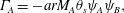 $$\begin{eqnarray}\displaystyle & \displaystyle \unicode[STIX]{x1D6E4}_{A}=-arM_{A}\unicode[STIX]{x1D703}_{s}\unicode[STIX]{x1D713}_{A}\unicode[STIX]{x1D713}_{B}, & \displaystyle\end{eqnarray}$$
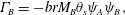 $$\begin{eqnarray}\displaystyle & \displaystyle \unicode[STIX]{x1D6E4}_{B}=-brM_{B}\unicode[STIX]{x1D703}_{s}\unicode[STIX]{x1D713}_{A}\unicode[STIX]{x1D713}_{B}, & \displaystyle\end{eqnarray}$$
 $$\begin{eqnarray}\displaystyle & \displaystyle \unicode[STIX]{x1D6E4}_{C}=crM_{C}\unicode[STIX]{x1D703}_{s}\unicode[STIX]{x1D713}_{A}\unicode[STIX]{x1D713}_{B}+\unicode[STIX]{x1D6FC}M_{C}\dot{\unicode[STIX]{x1D703}}_{s}, & \displaystyle\end{eqnarray}$$
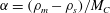 $\unicode[STIX]{x1D6FC}=(\unicode[STIX]{x1D70C}_{m}-\unicode[STIX]{x1D70C}_{s})/M_{C}$. Now that mass balance equations for the chemistry are established, mass balance equations for the multiphase solvent–membrane system are needed.
A simple but necessary assumption is that our volume is occupied by only solvent and membrane, i.e. there are no ‘voids’. This no-void assumption implies
 $$\begin{eqnarray}\unicode[STIX]{x1D703}_{s}+\unicode[STIX]{x1D703}_{m}=1\end{eqnarray}$$
everywhere. Mass balances for the solvent and membrane phases provide
 $$\begin{eqnarray}\displaystyle & \displaystyle \frac{\unicode[STIX]{x2202}(\unicode[STIX]{x1D70C}_{s}\unicode[STIX]{x1D703}_{s})}{\unicode[STIX]{x2202}t}+\unicode[STIX]{x1D735}\boldsymbol{\cdot }(\unicode[STIX]{x1D70C}_{s}\unicode[STIX]{x1D703}_{s}\boldsymbol{v}_{s})=R_{s}, & \displaystyle\end{eqnarray}$$
 $$\begin{eqnarray}\displaystyle & \displaystyle \frac{\unicode[STIX]{x2202}(\unicode[STIX]{x1D70C}_{m}\unicode[STIX]{x1D703}_{m})}{\unicode[STIX]{x2202}t}=R_{m}, & \displaystyle\end{eqnarray}$$
 where  $R_{i}$ denotes the rate of mass added to phase
  $i$. Equation (2.24) has no advective term since the membrane is assumed to be immobile.
To ensure conservation of total mass, the rates  $R_{m}$ and
  $R_{s}$ must be related. To derive this relationship, let
  $V_{0}$ be an arbitrary control volume. The total mass (of all components) in
  $V_{0}$ is
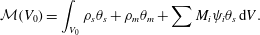 $$\begin{eqnarray}{\mathcal{M}}(V_{0})=\int _{V_{0}}\unicode[STIX]{x1D70C}_{s}\unicode[STIX]{x1D703}_{s}+\unicode[STIX]{x1D70C}_{m}\unicode[STIX]{x1D703}_{m}+\sum M_{i}\unicode[STIX]{x1D713}_{i}\unicode[STIX]{x1D703}_{s}\,\text{d}V.\end{eqnarray}$$
 Summing the five mass balance equations, (2.18)–(2.20) and (2.23)–(2.24), integrating over  $V_{0}$ and applying the divergence theorem gives
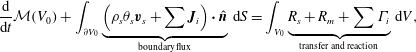 $$\begin{eqnarray}\frac{\text{d}}{\text{d}t}{\mathcal{M}}(V_{0})+\int _{\unicode[STIX]{x2202}V_{0}}\underbrace{\left(\unicode[STIX]{x1D70C}_{s}\unicode[STIX]{x1D703}_{s}\boldsymbol{v}_{s}+\sum \boldsymbol{J}_{i}\right)\boldsymbol{\cdot }\hat{\boldsymbol{n}}}_{\text{boundary flux}}\,\text{d}S=\int _{V_{0}}\underbrace{R_{s}+R_{m}+\sum \unicode[STIX]{x1D6E4}_{i}}_{\text{transfer}\;\text{and}\;\text{reaction}}\,\text{d}V,\end{eqnarray}$$
 where  $\hat{\boldsymbol{n}}$ is the outward unit normal vector. Summing (2.21) and applying (2.14) gives
  $\sum \unicode[STIX]{x1D6E4}_{i}=\unicode[STIX]{x1D6FC}M_{C}\dot{\unicode[STIX]{x1D703}}_{s}$. For the sake of obtaining a relationship between
  $R_{s}$ and
  $R_{m}$, briefly consider the case of zero boundary flux. Then, to conserve total mass within any control volume, we must have
  $R_{s}+R_{m}+\unicode[STIX]{x1D6FC}M_{C}\dot{\unicode[STIX]{x1D703}}_{s}=0$ holding point-wise. Substituting the value of
  $\unicode[STIX]{x1D6FC}$ in (2.16), using the no-void assumption (2.22) and the definition of
  $R_{m}$ in (2.24) gives
 $$\begin{eqnarray}R_{s}=-\frac{\unicode[STIX]{x1D70C}_{s}}{\unicode[STIX]{x1D70C}_{m}}\,R_{m}.\end{eqnarray}$$
This relationship is required for overall mass conservation.
Now consider the so-called Darcy velocity field  $\boldsymbol{q}_{s}=\unicode[STIX]{x1D703}_{s}\boldsymbol{v}_{s}$. Substituting the value of
  $R_{s}$ from (2.27) into (2.23), using a consequence of the no-void assumption (
 $\dot{\unicode[STIX]{x1D703}}_{s}=-\dot{\unicode[STIX]{x1D703}}_{m}$) and substituting
  $R_{m}$ by its value in (2.23) implies that the fluid Darcy velocity is divergence free,
 $$\begin{eqnarray}\unicode[STIX]{x1D735}\boldsymbol{\cdot }\boldsymbol{q}_{s}=0\end{eqnarray}$$
 and therefore the multiphase material is incompressible. Now return to (2.26) and consider the entire domain  $\unicode[STIX]{x1D6FA}$ with total mass
  ${\mathcal{M}}={\mathcal{M}}(\unicode[STIX]{x1D6FA})$. From the above argument, the right-hand side of this equation vanishes as a necessary condition on mass conservation. Then applying incompressibility (2.28), gives the total mass balance
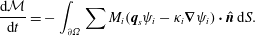 $$\begin{eqnarray}\frac{\text{d}{\mathcal{M}}}{\text{d}t}=-\int _{\unicode[STIX]{x2202}\unicode[STIX]{x1D6FA}}\sum M_{i}(\boldsymbol{q}_{s}\unicode[STIX]{x1D713}_{i}-\unicode[STIX]{x1D705}_{i}\unicode[STIX]{x1D735}\unicode[STIX]{x1D713}_{i})\boldsymbol{\cdot }\hat{\boldsymbol{n}}\,\text{d}S.\end{eqnarray}$$
As expressed in this equation, the total mass of the system is conserved as long as the chemical flux at the boundary vanishes. More generally, the total mass of the system can change according to how much chemical mass is being injected or removed via the boundary flux terms.
We now specify our choice for the form for the precipitation term  $R_{m}$. Although complicated models of precipitation exist (Matsue et al. Reference Matsue, Itatani, Fang, Shimizu, Unoura and Nabika2018; Ostapienko, Lopez & Komarova Reference Ostapienko, Lopez and Komarova2019), we employ a simple model in which the rate of membrane mass growth is proportional to the amount of product, provided that the product concentration exceeds some precipitation threshold, i.e.
 $$\begin{eqnarray}R_{m}=\unicode[STIX]{x1D6FD}\unicode[STIX]{x1D713}_{C}\unicode[STIX]{x1D703}_{s}{\mathcal{H}}(\unicode[STIX]{x1D713}_{C}-\unicode[STIX]{x1D713}_{C}^{\ast }),\end{eqnarray}$$
 where  $\unicode[STIX]{x1D6FD}$ is a rate constant,
  ${\mathcal{H}}$ is the standard Heaviside function and
  $\unicode[STIX]{x1D713}_{C}^{\ast }$ is the concentration threshold for precipitation to occur.
2.3 Momentum balance equations
Since inertial effects are assumed negligible ( $Re\ll 1$), the solvent momentum balance can be written as
 $$\begin{eqnarray}\unicode[STIX]{x1D735}\boldsymbol{\cdot }\unicode[STIX]{x1D64F}-\unicode[STIX]{x1D703}_{s}\unicode[STIX]{x1D735}P-\unicode[STIX]{x1D709}\boldsymbol{v}_{s}=\mathbf{0},\end{eqnarray}$$
 where  $\unicode[STIX]{x1D64F}$ is the multiphase stress tensor,
  $P$ is a so-called common pressure that is shared by the fluid and membrane phases (Cogan & Guy Reference Cogan and Guy2010) and
  $\unicode[STIX]{x1D709}$ is a friction coefficient which depends on volume fraction. Deviating slightly from the predominant multiphase literature, we chose the form of the stress tensor as
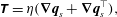 $$\begin{eqnarray}\unicode[STIX]{x1D64F}=\unicode[STIX]{x1D702}(\unicode[STIX]{x1D735}\boldsymbol{q}_{s}+\unicode[STIX]{x1D735}\boldsymbol{q}_{s}^{\top }),\end{eqnarray}$$
 where  $\unicode[STIX]{x1D702}$ is the fluid viscosity. In particular, since
  $\boldsymbol{q}_{s}=\unicode[STIX]{x1D703}_{s}\boldsymbol{v}_{s}$, we have placed the fluid volume fraction
  $\unicode[STIX]{x1D703}_{s}$ inside the gradient, whereas many multiphase models place the
  $\unicode[STIX]{x1D703}_{s}$ outside of the gradient but inside the divergence (Byrne & Preziosi Reference Byrne and Preziosi2003; Cogan & Keener Reference Cogan and Keener2005; Cogan & Guy Reference Cogan and Guy2010). Such a choice must be made for model closure, and neither is fully justified by first principles. We make the choice above to obtain equivalence to the Brinkman system (Brinkman Reference Brinkman1949), as discussed further below.
Indeed, applying incompressibility of the Darcy velocity to (2.31) simplifies it to a Brinkman equation with variable coefficients
 $$\begin{eqnarray}\unicode[STIX]{x1D702}\unicode[STIX]{x1D6FB}^{2}\boldsymbol{q}_{s}-\frac{\unicode[STIX]{x1D709}}{\unicode[STIX]{x1D703}_{s}}\boldsymbol{q}_{s}=\unicode[STIX]{x1D703}_{s}\unicode[STIX]{x1D735}P.\end{eqnarray}$$
 Note that (2.33) does not have any cross-derivative terms that would appear if the traditional multiphase stress tensor were used (Cogan & Guy Reference Cogan and Guy2010; Keener, Sircar & Fogelson Reference Keener, Sircar and Fogelson2011). Because the membrane is assumed immobile ( $\boldsymbol{v}_{m}\equiv \mathbf{0}$), no momentum equation is needed for it.
We emphasize that our choice of stress tensor in (2.32), which is slightly unconventional in the multiphase literature, is responsible for producing equivalence to the Brinkman system. The Brinkman equations were originally formulated in 1949 (Brinkman Reference Brinkman1949) and, since then, have undergone fundamental theoretical development (Childress Reference Childress1972) in close cooperation with experimental measurements (Neale & Nader Reference Neale and Nader1974), and, in recent decades, numerical simulation (Ochoa-Tapia & Whitaker Reference Ochoa-Tapia and Whitaker1995; Mu, Wang & Ye Reference Mu, Wang and Ye2014). We will demonstrate in § 3.2 that this system produces the expected no-slip behaviour on a fully formed membrane. It is interesting that, with the above modification, the modern multiphase averaging framework can be made to produce the Brinkman system, and therefore is consistent with 70 years of research on porous medium systems.
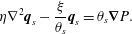
The friction coefficient  $\unicode[STIX]{x1D709}$ should be chosen in such a way that, at high membrane volume fraction, friction becomes the dominant effect in (2.33). The choice made here, and mentioned briefly in Leiderman & Fogelson (Reference Leiderman and Fogelson2013), is to use the Kozeny–Carman (KC) formula for permeability as it depends on porosity (Dullien Reference Dullien2012). In the present notation, the KC relationship gives the friction coefficient as
 $$\begin{eqnarray}\unicode[STIX]{x1D709}_{KC}(\unicode[STIX]{x1D703}_{s})=h\frac{(1-\unicode[STIX]{x1D703}_{s})^{2}}{\unicode[STIX]{x1D703}_{s}},\end{eqnarray}$$
 where  $h$ is an arbitrary constant. This friction coefficient will provide the desired no-slip behaviour in the membrane limit
  $\unicode[STIX]{x1D703}_{m}\rightarrow 1$. Angot (Reference Angot1999) discusses the implications of a similar singular friction term in a Brinkman system, although their model does not include the solvent volume fraction term in front of the pressure gradient and only applies to domains with spatially discontinuous volume fractions; the current fluid–membrane model generalizes this notion by being able to account for smooth spatial and temporal gradients in the volume fraction.
As an alternative to the singular  $\unicode[STIX]{x1D709}_{KC}$, the friction coefficient can be chosen to be a (non-singular) Hill function, as used in Leiderman & Fogelson (Reference Leiderman and Fogelson2011, Reference Leiderman and Fogelson2013),
 $$\begin{eqnarray}\unicode[STIX]{x1D709}_{H}(\unicode[STIX]{x1D703}_{s})=h\frac{(1-\unicode[STIX]{x1D703}_{s})^{n}}{K^{n}+(1-\unicode[STIX]{x1D703}_{s})^{n}}.\end{eqnarray}$$
 The use of Hill functions is largely empirical, although it has significant advantages in that it is finite in the membrane limit and therefore more numerically stable. Additionally,  $K$ determines the half-saturation point and
  $n$ indicates the qualitative manner at which this saturation is achieved. These parameters allow for fine-tuning to specific experimental observations.
Finally, a friction term employed in many biofilm multiphase models is
 $$\begin{eqnarray}\unicode[STIX]{x1D709}_{B}(\unicode[STIX]{x1D703}_{s})=h\unicode[STIX]{x1D703}_{s}(1-\unicode[STIX]{x1D703}_{s}).\end{eqnarray}$$
 This choice has become popular in the literature (Byrne & Preziosi Reference Byrne and Preziosi2003; Cogan & Keener Reference Cogan and Keener2004, Reference Cogan and Keener2005; Cogan & Guy Reference Cogan and Guy2010; Sorribes et al. Reference Sorribes, Moore, Byrne and Jain2019), and is often justified by the idea that friction should vanish if either phase,  $\unicode[STIX]{x1D703}_{s}$ or
  $\unicode[STIX]{x1D703}_{m}$, is absent. While it is an intuitive notion, we will show in § 3.2 that this friction coefficient does not produce the physically realistic behaviour of no-slip velocity on fully developed solid surfaces. To produce this behaviour, it is necessary that friction dominates, not vanishes, in the limit
  $\unicode[STIX]{x1D703}_{m}\rightarrow 1$.
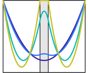
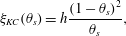
A visual comparison of these three friction coefficients is shown in figure 3. For the sake of comparison, we have chosen the constant  $h$ so that the three curves intersect at a reference porosity
  $\unicode[STIX]{x1D703}_{s}^{\ast }$, i.e.
  $\unicode[STIX]{x1D709}(\unicode[STIX]{x1D703}_{s}^{\ast })=\unicode[STIX]{x1D709}^{\ast }$. For
  $\unicode[STIX]{x1D709}^{\ast }=3$,
  $\unicode[STIX]{x1D703}_{s}^{\ast }=0.3$, this condition generates the constants
  $h_{KC}\approx 1.8$,
  $h_{H}\approx 4.5$ (
 $K=0.5$,
  $n=2$) and
  $h_{B}\approx 14.3$. For
  $\unicode[STIX]{x1D709}_{KC}$ and
  $\unicode[STIX]{x1D709}_{H}$, the value
  $\unicode[STIX]{x1D703}_{s}^{\ast }$ can be interpreted as the percolation threshold, i.e. the critical porosity below which the medium essentially behaves as impermeable to flow (Golden Reference Golden1997).
Figure 3. Comparison of friction terms  $\unicode[STIX]{x1D709}$.
  $\unicode[STIX]{x1D709}_{KC}$ (solid) is singular in the limit
  $\unicode[STIX]{x1D703}_{s}\rightarrow 0$,
  $\unicode[STIX]{x1D709}_{H}$ (dash) is non-singular in the porous limit (
 $K=0.5$,
  $n=2$) and
  $\unicode[STIX]{x1D709}_{B}$ (dot) yields maximum friction when both phases are present in equal amounts. All terms have been normalized by choosing
  $h$ such that
  $\unicode[STIX]{x1D709}(\unicode[STIX]{x1D703}_{S}^{\ast })=\unicode[STIX]{x1D709}^{\ast }$.
2.4 Model summary
The governing equations are now summarized for the reader. Rearranging (2.18)–(2.20) and applying incompressibility of  $\boldsymbol{q}_{s}=\unicode[STIX]{x1D703}_{s}\boldsymbol{v}_{s}$ gives the following ADR evolution equations for aqueous chemical concentration:
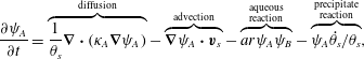 $$\begin{eqnarray}\displaystyle & \displaystyle \frac{\unicode[STIX]{x2202}\unicode[STIX]{x1D713}_{A}}{\unicode[STIX]{x2202}t}=\overbrace{\frac{1}{\unicode[STIX]{x1D703}_{s}}\unicode[STIX]{x1D735}\boldsymbol{\cdot }(\unicode[STIX]{x1D705}_{A}\unicode[STIX]{x1D735}\unicode[STIX]{x1D713}_{A})}^{\text{diffusion}}-\overbrace{\unicode[STIX]{x1D735}\unicode[STIX]{x1D713}_{A}\boldsymbol{\cdot }\boldsymbol{v}_{s}}^{\text{advection}}-\overbrace{ar\unicode[STIX]{x1D713}_{A}\unicode[STIX]{x1D713}_{B}}^{\substack{ \text{aqueous} \\ \text{reaction}}}-\overbrace{\unicode[STIX]{x1D713}_{A}\dot{\unicode[STIX]{x1D703}}_{s}/\unicode[STIX]{x1D703}_{s}}^{\substack{ \text{precipitate} \\ \text{reaction}}}, & \displaystyle\end{eqnarray}$$
 $$\begin{eqnarray}\displaystyle & \displaystyle \frac{\unicode[STIX]{x2202}\unicode[STIX]{x1D713}_{B}}{\unicode[STIX]{x2202}t}=\frac{1}{\unicode[STIX]{x1D703}_{s}}\unicode[STIX]{x1D735}\boldsymbol{\cdot }(\unicode[STIX]{x1D705}_{B}\unicode[STIX]{x1D735}\unicode[STIX]{x1D713}_{B})-\unicode[STIX]{x1D735}\unicode[STIX]{x1D713}_{B}\boldsymbol{\cdot }\boldsymbol{v}_{s}-br\unicode[STIX]{x1D713}_{A}\unicode[STIX]{x1D713}_{B}-\unicode[STIX]{x1D713}_{B}\dot{\unicode[STIX]{x1D703}}_{s}/\unicode[STIX]{x1D703}_{s}, & \displaystyle\end{eqnarray}$$
 $$\begin{eqnarray}\displaystyle & \displaystyle \frac{\unicode[STIX]{x2202}\unicode[STIX]{x1D713}_{C}}{\unicode[STIX]{x2202}t}=\frac{1}{\unicode[STIX]{x1D703}_{s}}\unicode[STIX]{x1D735}\boldsymbol{\cdot }(\unicode[STIX]{x1D705}_{C}\unicode[STIX]{x1D735}\unicode[STIX]{x1D713}_{C})-\unicode[STIX]{x1D735}\unicode[STIX]{x1D713}_{C}\boldsymbol{\cdot }\boldsymbol{v}_{s}+cr\unicode[STIX]{x1D713}_{A}\unicode[STIX]{x1D713}_{B}-(\unicode[STIX]{x1D713}_{C}-\unicode[STIX]{x1D6FC})\dot{\unicode[STIX]{x1D703}}_{s}/\unicode[STIX]{x1D703}_{s}, & \displaystyle\end{eqnarray}$$
 where  $\unicode[STIX]{x1D6FC}=(\unicode[STIX]{x1D70C}_{m}-\unicode[STIX]{x1D70C}_{s})/M_{C}$. Meanwhile, the evolution equations for the fluid and solid phases can be summarized as
 $$\begin{eqnarray}\displaystyle & \displaystyle \unicode[STIX]{x1D703}_{s}+\unicode[STIX]{x1D703}_{m}=1, & \displaystyle\end{eqnarray}$$
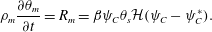 $$\begin{eqnarray}\displaystyle & \displaystyle \unicode[STIX]{x1D70C}_{m}\frac{\unicode[STIX]{x2202}\unicode[STIX]{x1D703}_{m}}{\unicode[STIX]{x2202}t}=R_{m}=\unicode[STIX]{x1D6FD}\unicode[STIX]{x1D713}_{C}\unicode[STIX]{x1D703}_{s}{\mathcal{H}}(\unicode[STIX]{x1D713}_{C}-\unicode[STIX]{x1D713}_{C}^{\ast }). & \displaystyle\end{eqnarray}$$
The momentum equation is a Brinkman equation with variable permeability
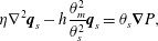 $$\begin{eqnarray}\displaystyle & \displaystyle \unicode[STIX]{x1D702}\unicode[STIX]{x1D6FB}^{2}\boldsymbol{q}_{s}-h\frac{\unicode[STIX]{x1D703}_{m}^{2}}{\unicode[STIX]{x1D703}_{s}^{2}}\boldsymbol{q}_{s}=\unicode[STIX]{x1D703}_{s}\unicode[STIX]{x1D735}P, & \displaystyle\end{eqnarray}$$
 $$\begin{eqnarray}\displaystyle & \displaystyle \unicode[STIX]{x1D735}\boldsymbol{\cdot }\boldsymbol{q}_{s}=0, & \displaystyle\end{eqnarray}$$
 where we have employed the  $\unicode[STIX]{x1D709}_{KC}$ friction term. We will now consider these coupled PDEs in a simplified setting that will permit exact solutions.
3 Analysis of reduced model
Analysis of any complicated system is aided by reduction into a form that is analytically tractable. Inspired by microfluidic experiments, we assume that some chemostat controls the influx of reactants’ molarity far upstream. All variables are kept constant along the longitudinal axis by neglecting diffusion and assuming parallel flow. This requirement of parallel flow also means that the reaction takes place everywhere along the longitudinal axis simultaneously. Finally, we assume that the precipitation threshold is negligible. These assumptions approximately model the fast time scale, initial membrane growth observed in the experiments shown in figure 1 for a single transverse cross-section of the domain; the slow time scale membrane thickening is diffusion controlled, and therefore we do not seek to capture it in this analysis.
Applying these assumptions to the governing equations reduces the system considerably so that it becomes a Poiseuille analysis; these assumptions generate the following reduced system:
 $$\begin{eqnarray}\displaystyle & \displaystyle \dot{\unicode[STIX]{x1D713}}_{C}=cr\unicode[STIX]{x1D713}_{A}\unicode[STIX]{x1D713}_{B}-(\unicode[STIX]{x1D713}_{C}-\unicode[STIX]{x1D6FC})\dot{\unicode[STIX]{x1D703}}_{s}/\unicode[STIX]{x1D703}_{s}, & \displaystyle\end{eqnarray}$$
 $$\begin{eqnarray}\displaystyle & \displaystyle \unicode[STIX]{x1D703}_{s}+\unicode[STIX]{x1D703}_{m}=1, & \displaystyle\end{eqnarray}$$
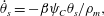 $$\begin{eqnarray}\displaystyle & \displaystyle \dot{\unicode[STIX]{x1D703}}_{s}=-\unicode[STIX]{x1D6FD}\unicode[STIX]{x1D713}_{C}\unicode[STIX]{x1D703}_{s}/\unicode[STIX]{x1D70C}_{m}, & \displaystyle\end{eqnarray}$$
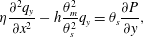 $$\begin{eqnarray}\displaystyle & \displaystyle \unicode[STIX]{x1D702}\frac{\unicode[STIX]{x2202}^{2}q_{y}}{\unicode[STIX]{x2202}x^{2}}-h\frac{\unicode[STIX]{x1D703}_{m}^{2}}{\unicode[STIX]{x1D703}_{s}^{2}}q_{y}=\unicode[STIX]{x1D703}_{s}\frac{\unicode[STIX]{x2202}P}{\unicode[STIX]{x2202}y}, & \displaystyle\end{eqnarray}$$
 $\unicode[STIX]{x1D713}_{C}$,
  $\unicode[STIX]{x1D703}_{s}$,
  $\unicode[STIX]{x1D703}_{m}$,
  $q_{y}$ and
  $\unicode[STIX]{x2202}_{y}P$ are unknown. The pressure gradient
  $\unicode[STIX]{x2202}_{y}P$ is determined by requiring a constant total flux for all time (see (3.11)). Note that the longitudinal axis is chosen to be
  $y$ such that only this component of the Darcy velocity
  $\boldsymbol{q}_{s}=q_{x}\hat{\boldsymbol{x}}+q_{y}\hat{\boldsymbol{y}}$ remains. In § 3.1 we obtain an analytic estimate on the rate of membrane formation by treating
  $\unicode[STIX]{x1D713}_{C}$ and
  $\unicode[STIX]{x1D703}_{m}$ as a planar dynamical system. Then in § 3.2 we solve equations (3.1) with a combination of analytic and numerical methods to visualize how the membrane affects the flow profile in time.
3.1 Fixed point analysis
Our approach is to linearize the reduced model system, then perform an eigenvalue analysis about a steady state fixed point. The benefit of this is the eigenvalue gives an approximate estimate to the rate that membrane develops, a quantity that is possible to measure experimentally.
Before doing a fixed point analysis, it is helpful to understand the conditions on which the existence and stability of fixed points depends. To do so, eliminate the explicit dependence of  $\dot{\unicode[STIX]{x1D713}}_{C}$ on volume fraction and replace all
  $\dot{\unicode[STIX]{x1D703}}_{s}$ in (3.1a) with (3.1c) to obtain a quadratic ODE of the form
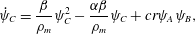 $$\begin{eqnarray}\dot{\unicode[STIX]{x1D713}}_{C}=\frac{\unicode[STIX]{x1D6FD}}{\unicode[STIX]{x1D70C}_{m}}\unicode[STIX]{x1D713}_{C}^{2}-\frac{\unicode[STIX]{x1D6FC}\unicode[STIX]{x1D6FD}}{\unicode[STIX]{x1D70C}_{m}}\unicode[STIX]{x1D713}_{C}+cr\unicode[STIX]{x1D713}_{A}\unicode[STIX]{x1D713}_{B},\end{eqnarray}$$
 which is an ODE in time alone, as the  $x\text{-dependences}$ of
  $\unicode[STIX]{x1D713}_{A}$ and
  $\unicode[STIX]{x1D713}_{B}$ are determined by the initial conditions. Examining the qualitative behaviour of this ODE by considering
  $\dot{\unicode[STIX]{x1D713}}_{C}=\dot{\unicode[STIX]{x1D713}}_{C}(\unicode[STIX]{x1D713}_{C})$, it is quadratic in
  $\unicode[STIX]{x1D713}_{C}$, intercepts the
  $\dot{\unicode[STIX]{x1D713}}_{C}$ axis at
  $cr\unicode[STIX]{x1D713}_{A}\unicode[STIX]{x1D713}_{B}\geqslant 0$, is concave up and has equilibria at
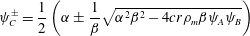 $$\begin{eqnarray}\unicode[STIX]{x1D713}_{C}^{\pm }=\frac{1}{2}\left(\unicode[STIX]{x1D6FC}\pm \frac{1}{\unicode[STIX]{x1D6FD}}\sqrt{\unicode[STIX]{x1D6FC}^{2}\unicode[STIX]{x1D6FD}^{2}-4cr\unicode[STIX]{x1D70C}_{m}\unicode[STIX]{x1D6FD}\unicode[STIX]{x1D713}_{A}\unicode[STIX]{x1D713}_{B}}\right)\end{eqnarray}$$
whose existence depends on the sign of
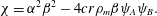 $$\begin{eqnarray}\unicode[STIX]{x1D712}=\unicode[STIX]{x1D6FC}^{2}\unicode[STIX]{x1D6FD}^{2}-4cr\unicode[STIX]{x1D70C}_{m}\unicode[STIX]{x1D6FD}\unicode[STIX]{x1D713}_{A}\unicode[STIX]{x1D713}_{B}.\end{eqnarray}$$
 If  $\unicode[STIX]{x1D712}>0$, equation (3.2) will have two fixed points, for
  $\unicode[STIX]{x1D712}=0$ these fixed points coalesce, and for
  $\unicode[STIX]{x1D712}<0$ there are no fixed points and
  $\dot{\unicode[STIX]{x1D713}}_{C}$ will grow without bound; see figure 4(a).
We now ask the question of whether fixed points exist in the reduced system, i.e.  $\unicode[STIX]{x1D712}\geqslant 0$ or
  $\unicode[STIX]{x1D6FC}^{2}\unicode[STIX]{x1D6FD}\geqslant 4cr\unicode[STIX]{x1D70C}_{m}\unicode[STIX]{x1D713}_{A}\unicode[STIX]{x1D713}_{B}$? We interpret this condition based on the physical meaning of the parameters:
  $\unicode[STIX]{x1D6FC}=(\unicode[STIX]{x1D70C}_{m}-\unicode[STIX]{x1D70C}_{s})/M_{C}$ has dimension of molarity and is
  $O$(10 M) where M refers to molar units,
  $1~\text{M}=1~\text{mol}~\text{l}^{-1}$; for example, using the reaction system in the introduction gives
  $\unicode[STIX]{x1D6FC}\approx 30~\text{M}$. We note that a similar analysis also justifies neglecting the precipitation threshold
  $\unicode[STIX]{x1D713}_{C}^{\ast }$, as
  $\unicode[STIX]{x1D713}_{C}^{\ast }\approx 0.001~\text{M}$. Although both
  $r$ and
  $\unicode[STIX]{x1D6FD}$ scale the rates of the aqueous and precipitate reactions, respectively, they have different units;
  $r$ has units of volume per time while
  $\unicode[STIX]{x1D6FD}$ has units of mass per time. Because experimental values of
  $r$ and
  $\unicode[STIX]{x1D6FD}$ are expensive to acquire, for the sake of this simplified analysis we will assume that
  $\unicode[STIX]{x1D6FD}\approx r\unicode[STIX]{x1D70C}_{m}$ such that their effects do not impact the sign
  $\unicode[STIX]{x1D712}$. The stoichiometric coefficient
  $c$ for
  $C(\text{aq})$ can be assumed
  $O(1)$. Finally, examine the reactants
  $\unicode[STIX]{x1D713}_{A}$ and
  $\unicode[STIX]{x1D713}_{B}$. Most experiments in microfluidic chambers use molar concentrations with an upper bound of
  $O(1~\text{M})$; for example, in Ding et al. (Reference Ding, Batista, Steinbock, Cartwright and Cardoso2016) the maximum concentration of reactants was 0.5 M. Therefore, using parameter values taken from experiments,
  $\unicode[STIX]{x1D712}>0$ and fixed points exist for the reduced system.
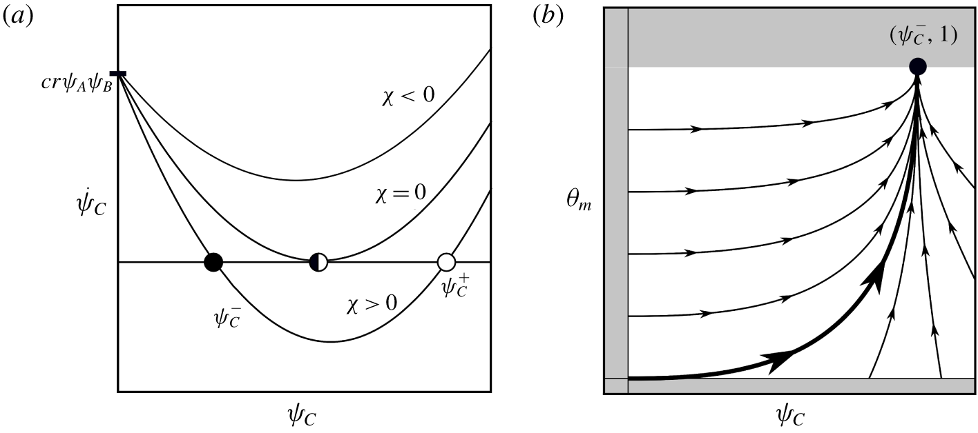
Figure 4. Dynamical system for  $\unicode[STIX]{x1D713}_{C}$ and
  $\unicode[STIX]{x1D703}_{m}$. (a) Qualitative stability of
  $\dot{\unicode[STIX]{x1D713}}_{C}(\unicode[STIX]{x1D713}_{C})$ ODE. The left equilibrium
  $\unicode[STIX]{x1D713}_{C}^{-}$ is stable and exists for
  $\unicode[STIX]{x1D712}\geqslant 0$. (b) Visualization of planar dynamical system approaching the fixed point
  $(\unicode[STIX]{x1D713}_{C}^{-},1)$ for
  $\unicode[STIX]{x1D712}>0$. The thicker line corresponds to homogeneous initial conditions for
  $\unicode[STIX]{x1D713}_{C}$ and
  $\unicode[STIX]{x1D703}_{m}$. Shaded region is outside of the domain of
  $(\unicode[STIX]{x1D713}_{C},\unicode[STIX]{x1D703}_{m})\in [0,\infty )\times [0,1]$.
We now consider the planar dynamical system in phase space  $(\unicode[STIX]{x1D713}_{C},\unicode[STIX]{x1D703}_{m})\in [0,\infty )\times [0,1]$ with fixed point
  $(\unicode[STIX]{x1D713}_{C}^{-},1)$. The dynamical system is
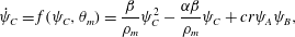 $$\begin{eqnarray}\displaystyle & \displaystyle \dot{\unicode[STIX]{x1D713}}_{C}=f(\unicode[STIX]{x1D713}_{C},\unicode[STIX]{x1D703}_{m})=\frac{\unicode[STIX]{x1D6FD}}{\unicode[STIX]{x1D70C}_{m}}\unicode[STIX]{x1D713}_{C}^{2}-\frac{\unicode[STIX]{x1D6FC}\unicode[STIX]{x1D6FD}}{\unicode[STIX]{x1D70C}_{m}}\unicode[STIX]{x1D713}_{C}+cr\unicode[STIX]{x1D713}_{A}\unicode[STIX]{x1D713}_{B}, & \displaystyle\end{eqnarray}$$
 $$\begin{eqnarray}\displaystyle & \displaystyle \dot{\unicode[STIX]{x1D703}}_{m}=g(\unicode[STIX]{x1D713}_{C},\unicode[STIX]{x1D703}_{m})=\unicode[STIX]{x1D6FD}\unicode[STIX]{x1D713}_{C}(1-\unicode[STIX]{x1D703}_{m})/\unicode[STIX]{x1D70C}_{m}, & \displaystyle\end{eqnarray}$$
 $r$,
$r$,  $c$,
$c$,  $\unicode[STIX]{x1D70C}_{m}$,
  $\unicode[STIX]{x1D6FC}$,
  $\unicode[STIX]{x1D6FD}$,
  $\unicode[STIX]{x1D713}_{A}$ and
  $\unicode[STIX]{x1D713}_{B}$ are assumed to be known and constant. The eigenvalues of the Jacobian generated by (3.5) evaluated at the fixed points provide information about the rate of growth of
  $\unicode[STIX]{x1D713}_{C}$ and
  $\unicode[STIX]{x1D703}_{m}$. This particular eigen-system is simple to interpret because the eigenvectors align with the coordinate axes and therefore the eigenvalues correspond to the rates that the physical variables
  $(\unicode[STIX]{x1D713}_{C},\unicode[STIX]{x1D703}_{m})$ approach their equilibria when close to the steady state. These rates are given by,
 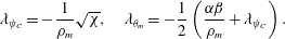 $$\begin{eqnarray}\unicode[STIX]{x1D706}_{\unicode[STIX]{x1D713}_{C}}=-\frac{1}{\unicode[STIX]{x1D70C}_{m}}\sqrt{\unicode[STIX]{x1D712}},\quad \unicode[STIX]{x1D706}_{\unicode[STIX]{x1D703}_{m}}=-\frac{1}{2}\left(\frac{\unicode[STIX]{x1D6FC}\unicode[STIX]{x1D6FD}}{\unicode[STIX]{x1D70C}_{m}}+\unicode[STIX]{x1D706}_{\unicode[STIX]{x1D713}_{C}}\right).\end{eqnarray}$$
 Both eigenvalues are negative, and therefore the fixed point is stable, because  $\unicode[STIX]{x1D6FC}\unicode[STIX]{x1D6FD}/\unicode[STIX]{x1D70C}_{m}+\unicode[STIX]{x1D706}_{\unicode[STIX]{x1D713}_{C}}=\unicode[STIX]{x1D6FC}\unicode[STIX]{x1D6FD}/\unicode[STIX]{x1D70C}_{m}-\sqrt{\unicode[STIX]{x1D712}}/\unicode[STIX]{x1D70C}_{m}>0$ always. For this same reason, it is true that
  $|\unicode[STIX]{x1D706}_{\unicode[STIX]{x1D703}_{m}}|<|\unicode[STIX]{x1D706}_{\unicode[STIX]{x1D713}_{C}}|$, meaning the membrane volume fraction approaches its fixed point at a slower rate than the aqueous product. This agrees with our intuition, as the conversion of
  $C(\text{aq})$ to
  $C(\text{s})$ means we would expect
  $\unicode[STIX]{x1D703}_{m}$ production to lag behind
  $\unicode[STIX]{x1D713}_{C}$.
3.2 Ricatti–Poiseuille analysis
We now solve system (3.1) to visualize the transition in solvent velocity from one- to two-channel flow. To summarize the approach, each equation in (3.1) is solved sequentially; equations (3.1a)–(3.1c) admit exact solutions while the fluid velocity in (3.1d) requires numerical solution. Although in this reduced case the location of the membrane is determined through the initial conditions  $\unicode[STIX]{x1D713}_{A}^{0}$ and
  $\unicode[STIX]{x1D713}_{B}^{0}$, and therefore known a priori, the fact that no interface boundary conditions are required demonstrates a considerable advantage of this model over more traditional approaches.
For initial conditions, let  $\unicode[STIX]{x1D713}_{C}(x,t)=0$ and
  $\unicode[STIX]{x1D703}_{s}(x,t)=1$. Fix the initial reagents by the piecewise-constant values
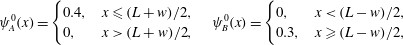 $$\begin{eqnarray}\unicode[STIX]{x1D713}_{A}^{0}(x)=\left\{\begin{array}{@{}ll@{}}0.4,\quad & x\leqslant (L+w)/2,\\ 0,\quad & x>(L+w)/2,\end{array}\right.\quad \unicode[STIX]{x1D713}_{B}^{0}(x)=\left\{\begin{array}{@{}ll@{}}0,\quad & x<(L-w)/2,\\ 0.3,\quad & x\geqslant (L-w)/2,\end{array}\right.\end{eqnarray}$$
 such that there is only a middle region of width  $w$ in
  $x\in (0,L)$ in which the reactants
  $A$ and
  $B$ are simultaneously present. We note that the following results hold for any choice of
  $\unicode[STIX]{x1D713}_{i}^{0}$, provided that
  $\unicode[STIX]{x1D712}(x)>0$.
Substituting (3.1c) into (3.1a) produces an ODE with quadratic nonlinearity known as the Ricatti equation. Despite being nonlinear, the Ricatti equation admits an exact solution for  $\unicode[STIX]{x1D713}_{C}(x,t)$ (see appendix A). Given
  $\unicode[STIX]{x1D713}_{A}^{0}(x)$ and
  $\unicode[STIX]{x1D713}_{B}^{0}(x)$, the solution to this Ricatti equation is,
 $$\begin{eqnarray}\unicode[STIX]{x1D713}_{C}(x,t)=\unicode[STIX]{x1D6FE}_{1}\unicode[STIX]{x1D6FE}_{2}\frac{\unicode[STIX]{x1D70C}_{m}}{\unicode[STIX]{x1D6FD}}\left(\frac{\text{e}^{\unicode[STIX]{x1D6FE}_{2}t}-\text{e}^{\unicode[STIX]{x1D6FE}_{1}t}}{\unicode[STIX]{x1D6FE}_{2}\text{e}^{\unicode[STIX]{x1D6FE}_{1}t}-\unicode[STIX]{x1D6FE}_{1}\text{e}^{\unicode[STIX]{x1D6FE}_{2}t}}\right),\end{eqnarray}$$
where
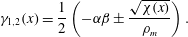 $$\begin{eqnarray}\unicode[STIX]{x1D6FE}_{1,2}(x)=\frac{1}{2}\left(-\unicode[STIX]{x1D6FC}\unicode[STIX]{x1D6FD}\pm \frac{\sqrt{\unicode[STIX]{x1D712}(x)}}{\unicode[STIX]{x1D70C}_{m}}\right).\end{eqnarray}$$
 In order to find the exact solution for  $\unicode[STIX]{x1D703}_{s}(x,t)$, we must use the fact that (3.1c) is separable. Then, because the antiderivative of
  $\unicode[STIX]{x1D713}_{C}$ can be given in terms of elementary functions, we can obtain an explicit formula for solvent volume fraction
  $\unicode[STIX]{x1D703}_{s}(x,t)$,
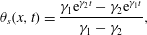 $$\begin{eqnarray}\unicode[STIX]{x1D703}_{s}(x,t)=\frac{\unicode[STIX]{x1D6FE}_{1}\text{e}^{\unicode[STIX]{x1D6FE}_{2}t}-\unicode[STIX]{x1D6FE}_{2}\text{e}^{\unicode[STIX]{x1D6FE}_{1}t}}{\unicode[STIX]{x1D6FE}_{1}-\unicode[STIX]{x1D6FE}_{2}},\end{eqnarray}$$
 where have implemented the initial condition  $\unicode[STIX]{x1D703}_{s}(x,0)=1$. Then, the membrane volume fraction
  $\unicode[STIX]{x1D703}_{m}(x,t)$ can be computed easily using the no-void assumption.
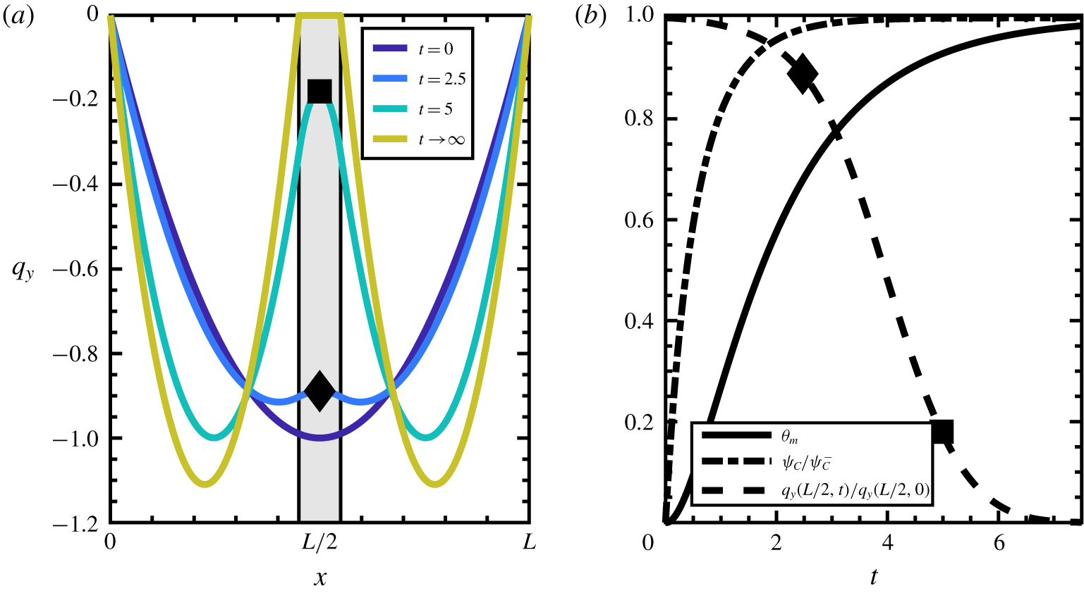
Figure 5. Developing membrane affects fluid flow. (a) Flow profile in a one-dimensional channel transitions from one-channel to two-channel flow. The reaction region is shaded. (b) Relevant variables evaluated in the reaction region at  $x=L/2$, normalized for legibility;
  $\unicode[STIX]{x1D713}_{C}$ develops first, followed by
  $\unicode[STIX]{x1D703}_{m}$, which when large enough triggers the transition from one- to two-channel flow. The percolation threshold
  $\unicode[STIX]{x1D703}_{s}^{\ast }$ is set to
  $\unicode[STIX]{x1D703}_{s}^{\ast }=0.3$, which is why negligible change in fluid velocity is seen until
  $\unicode[STIX]{x1D703}_{m}\approx 0.7$. The specific
  $\unicode[STIX]{x1D703}_{s}^{\ast }$ was chosen based on the maximum volume fraction of an arrangement of packed spheres in three dimensions (Conway & Sloane Reference Conway and Sloane2013). The black diamond and square represent the system state inside the reaction region at
  $t=2.5$ and
  $t=5$, respectively.
Until this point, all solutions in space have been treated independently. The effect of variations in space is taken into account when solving for the longitudinal component of the Darcy velocity,  $q_{y}$. We numerically solve the momentum equation (3.1d) for
  $q_{y}$ using a finite difference method. The
  $x$ domain is discretized into
  $N$ intervals of equal width
  $\unicode[STIX]{x0394}x=1/N$ such that
  $x_{j}=j\unicode[STIX]{x0394}x$,
  $j=1,\ldots ,N-1$, and use centred-difference approximations to the derivatives. Note that
  $q_{y}(x_{0})=q_{y}(x_{N})=0$ due to the no-slip boundary conditions. This discretization results in a tridiagonal linear system which can be solved in
  $O(N)$ complexity by using the Thomas algorithm (see Strikwerda Reference Strikwerda2004, pp. 78–79). The velocity is constrained to satisfy constant flux in accordance with experiments, which mathematically is represented by
 $$\begin{eqnarray}\int _{0}^{L}q_{y}\,\text{d}x=\text{const}.\end{eqnarray}$$
This constant-flux condition allows the computation of the required pressure gradient at each time step. The authors use the Julia programming language to solve the BVP (Bezanson et al. Reference Bezanson, Edelman, Karpinski and Shah2017).
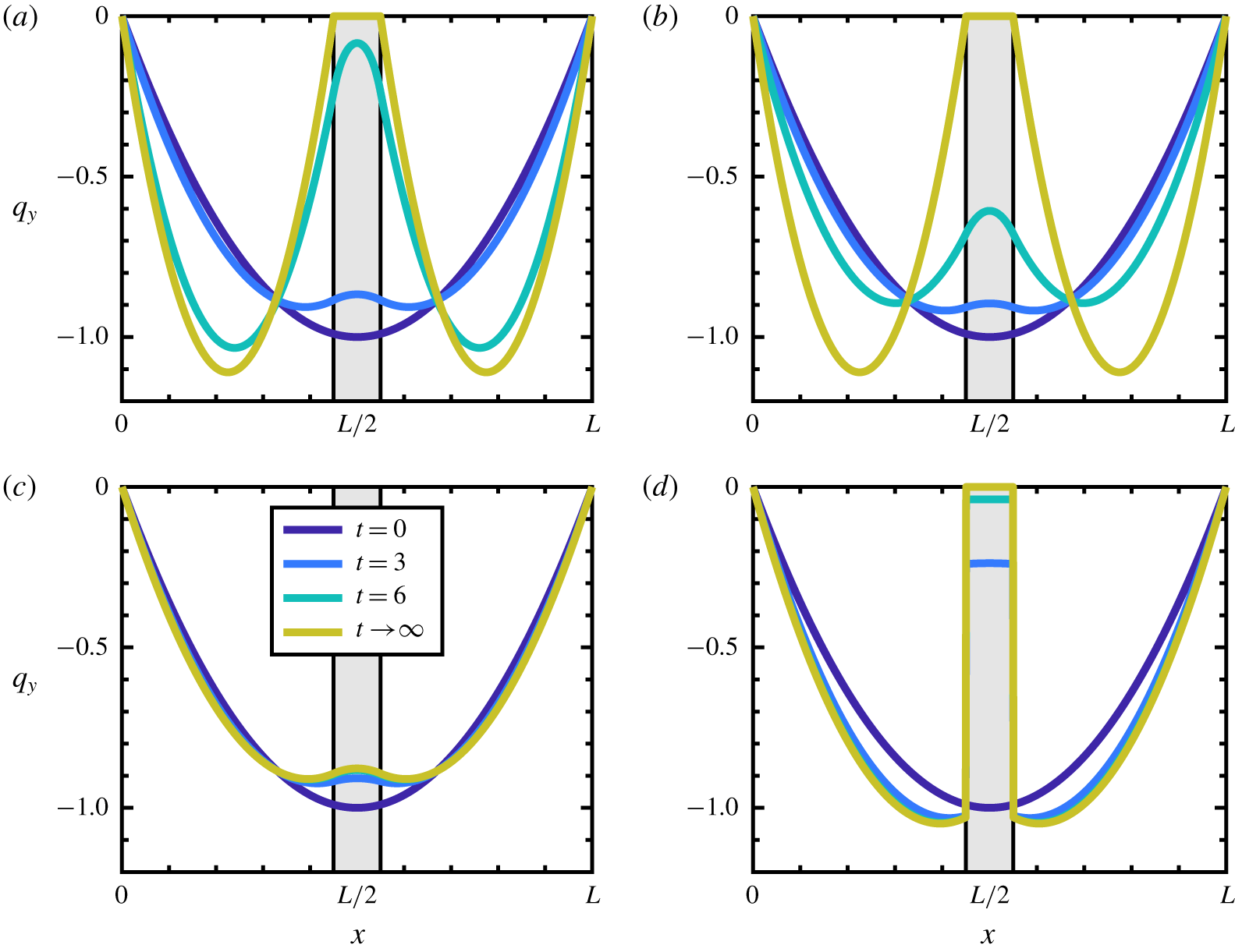
Figure 6. Comparison of different models. (a–c) Use the stress in (2.32) with the friction term given by (a) Kozeny–Carman, (b) Hill function and (c) the ‘biofilm’ term; (d) uses a conventional multiphase stress  $\unicode[STIX]{x1D64F}^{\prime }$ in (3.12) with
  $\unicode[STIX]{x1D709}_{B}$. The coefficients
  $h$ are scaled so as to make the three coefficients comparable in strength. The first two friction terms produce the desired no-slip on the membrane interface and the third, while affecting the fluid flow, does not generate the desired no-slip boundary condition. Additionally, the stress and friction combination used in (d), which is usually employed in multiphase models, does not yield the desired no-slip behaviour on the fluid–membrane interface.
The developing membrane for the one-dimensional reduced model geometry is shown in figure 5(a). Membrane develops within the shaded region, which in this example is 10 % of the domain. Because the membrane has finite width, the constant-flux condition causes the pressure gradient to increase with the developing membrane, causing the maximum speed for the two-channel flow to be slightly higher than the maximum speed for the one-channel flow. In this sense, the developing membrane splits the domain into two symmetric one-channel flows. This transition occurs without the need for boundary conditions at the fluid–membrane interface, indicated by the boundary of the shaded region.

Figure 7. Effect of increasing membrane thickness. As a percentage of the domain length, membrane width is (a) 5 %, (b) 15 % and (c) 33 %. The increasing maximum flow speed is due to the constant-flux constraint, and is analogous to that what would occur if the membrane boundaries and interface conditions were prescribed a priori in a single-phase flow.
Figure 5(b) shows the three main variables of the reduced model as functions of time, evaluated in the middle of the reaction region ( $x=L/2$). The
  $\unicode[STIX]{x1D713}_{C}$ variable increases immediately due to the presence of
  $\unicode[STIX]{x1D713}_{A}$ and
  $\unicode[STIX]{x1D713}_{B}$. The membrane initially has zero growth rate due to the absence of
  $\unicode[STIX]{x1D713}_{C}$, and grows at a slower rate than
  $\unicode[STIX]{x1D713}_{C}$. This ordering on the growth rates matches our expectations from the eigenvalue analysis of § 3.1. The
  $q_{y}$ curve demonstrates the transition from one-channel to two-channel pipe flow by measuring the normalized value in the middle of the pipe as a function of time. By comparing
  $q_{y}$ with
  $\unicode[STIX]{x1D703}_{m}$, one can see the effect of the percolation threshold
  $\unicode[STIX]{x1D703}_{s}^{\ast }=0.3$. After the solvent volume fraction declines past this value, the fluid velocity begins to respond strongly to precipitating membrane.
To be precise, we say a velocity displays ‘no-slip’ behaviour when, in the limit as a transition region between a fluid region ( $\unicode[STIX]{x1D703}_{s}=1$) and membrane region (
 $\unicode[STIX]{x1D703}_{s}=0$) becomes discontinuous (i.e. a ‘sharp interface’), the velocity goes to zero as one approaches the interface from the fluid region. In the case that the volume fraction is always discontinuous (as in this reduced model), this limit is achieved as the membrane fully develops, i.e.
  $\unicode[STIX]{x1D703}_{s}\rightarrow 0$, at the interface. Figure 6 demonstrates the effect of using different stresses and friction coefficients. Figure 6(a,b) demonstrates the desired no-slip behaviour in the membrane limit by using
  $\unicode[STIX]{x1D709}_{KC}$ and
  $\unicode[STIX]{x1D709}_{H}$, respectively. In figure 6(c) the effect of the friction coefficient
  $\unicode[STIX]{x1D709}_{B}$ is shown. While there is some effect on the flow profile,
  $\unicode[STIX]{x1D709}_{B}$ does not demonstrate the no-slip condition on the membrane. While the
  $\unicode[STIX]{x1D709}_{B}$ term was developed primarily for high-permeability applications, our framework was developed to capture the transition from purely fluid behaviour, to partially permeable, to a fully developed impermeable solid. As demonstrated, this full transition requires either the
  $\unicode[STIX]{x1D709}_{KC}$ or
  $\unicode[STIX]{x1D709}_{H}$ friction coefficient. Figure 6(d) displays the flow profile when using the multiphase stress tensor typically used in multiphase models,
 $$\begin{eqnarray}\unicode[STIX]{x1D64F}^{\prime }=\unicode[STIX]{x1D702}\unicode[STIX]{x1D703}_{f}(\unicode[STIX]{x1D735}\boldsymbol{v}_{s}+\unicode[STIX]{x1D735}\boldsymbol{v}_{s}^{\top })\end{eqnarray}$$
 given in Drew (Reference Drew1983) and Cogan & Guy (Reference Cogan and Guy2010) as well as the biofilm friction coefficient. Even at long times, the model using the above  $\unicode[STIX]{x1D64F}^{\prime }$ does not produce the desired no-slip at the fluid–membrane interface. Using
  $\unicode[STIX]{x1D64F}^{\prime }$ with other friction terms produces inconclusive results. It was this behaviour that motivated the authors to modify the stress term to the form given in (2.32), which has the additional advantage that it allows for a reduction of the momentum equation to the Brinkman form.
Figure 7 shows three flows with reaction regions of various sizes, and therefore different width of membranes. The initial flow profiles of all are equivalent, as the reaction has not yet occurred and no membrane is present. However, as membrane develops, the constant-flux condition requires that for regions with thicker membranes, the flow velocity must increase in the non-reacting regions to compensate for the loss of flux in the membrane region. These results demonstrate that, once the membrane is fully developed, the flow domain treats the membrane portion as a no-slip boundary and the prescribed constant-flux conditions lead to the expected results from single-phase fluids.
4 Conclusion
Typically, interface conditions on boundaries must be prescribed a priori when modelling fluid flows. However, motivated by microfluidic experiments of a precipitate reaction, there exist situations where solid materials develop dynamically and so the exact location of such a boundary is not known a priori. This situation exposes a deficiency in modelling techniques that rely on knowledge of where fluid–structure interfaces exist.
To formulate the model, we assumed conservation of mass for the entire chemistry–fluid–membrane system. The reacting chemical species were assumed to exist in the fluid phase as volumeless scalar fields subject to mass flux determined by a combination of advection with the fluid flow and diffusion down gradients in molarity. The careful consideration of changing solvent volume inside the domain led to extra terms being included in the reaction equations, and in particular conservation of mass for the entire system was used to determine the closure for the aqueous product’s reaction equation. A momentum equation for the fluid velocity followed the usual Cauchy stress formulation with the slight modification that all tensor quantities depend on the Darcy velocity  $\boldsymbol{q}_{s}=\unicode[STIX]{x1D703}_{s}\boldsymbol{v}_{s}$, not simply the tracer velocity
  $\boldsymbol{v}_{s}$ as is usual in the multiphase fluids literature. This choice, paired with incompressibility of the fluid Darcy velocity, led to a simplification of the momentum balance to a variable-coefficient Brinkman equation.
In order to demonstrate that the model reflects the expected behaviours, we first sought growth rate estimates from a linearized form of reduced equations. Then, to show that the dynamically generated no-slip boundary corresponded to development of the membrane, we performed what was essentially a Poiseuille analysis on the reduced model to show that the no-slip behaviour agreed qualitatively with expected behaviours, specifically the recovery of one-to-two channel transitions and the effect of membrane width paired with a constant-flux condition.
We examined three potential terms to be used in the momentum balance friction term, both by a direct comparison as functions of fluid volume fraction and by examining their effect on fluid flow from the perspective of how well they demonstrated no-slip behaviour. These results demonstrated that, qualitatively, the friction terms derived from Karman–Cozeny relationship and using Hill functions gave no-slip flow behaviour on the developed membrane. Additionally, the percolation threshold  $\unicode[STIX]{x1D703}_{s}^{\ast }$ can be chosen to reflect specific permeability properties of the structure under investigation. Both of these friction coefficients were preferable to the term commonly employed in biofilm models because
  $\unicode[STIX]{x1D709}_{B}$ does not recover the no-slip behaviour in low-permeability regions. Additionally, we briefly demonstrated that the usual multiphase stress does not result in the expected interface behaviour, which motivated our particular choice of stress.
To our knowledge, this is the first model that qualitatively captures the fluid–structure dynamics of a precipitate reaction in a low- $Re$ environment where the dynamically developing precipitate significantly affects the surrounding fluid flow. Future work will focus on numerical simulation of the full model in various geometries to be used as a predictive tool for experimentalists. In particular, exploring sufficient modelling conditions to generate the asymmetric growth in membrane in a two-dimensional setting analogous to the experimental microfluidic domains was something that we were not able to explore in this paper, as diffusion was ignored to reduce the model equations. A model capable of accurately capturing microfluidic experiments would be valuable to researchers using these devices to study precipitate reactions at the microscale and ultimately useful in examining origin of life theories.
Acknowledgements
P.S.E. is supported by the National Science Foundation (NSF) Graduate Research Fellowship under Grant 1449440. M.N.J.M. is supported by Simons Collaboration Grant 524259. N.G.C. is supported by NSF-CBET 1510743. Q.W. and O.S. are supported by NSF Grants 1609495 and 1565734.
Declaration of interests
The authors report no conflict of interest.
Appendix A. Solving Ricatti’s differential equation
The solution technique to Ricatti’s differential equation (see Tenenbaum & Pollard Reference Tenenbaum and Pollard1985, p. 97) is not very well known, so the derivation is stated here for the interested reader. A homogeneous first-order ODE is called a Ricatti equation if it is quadratic in the unknown, i.e.
 $$\begin{eqnarray}y^{\prime }(x)=q_{0}(x)+q_{1}(x)y(x)+q_{2}(x)y^{2}(x).\end{eqnarray}$$
 If  $q_{0}(x)\equiv 0$, this reduces to Bernoulli’s equation (see Tenenbaum & Pollard Reference Tenenbaum and Pollard1985, pp. 95–96). In general, one can transform Ricatti’s equation to an equivalent second-order linear differential equation. In this appendix, we detail this transformation and explicitly solve for the case of constant coefficients
  $q_{0}$,
  $q_{1}$ and
  $q_{2}$.
First, define a new variable  $v$ by
 $$\begin{eqnarray}v=q_{2}y,\end{eqnarray}$$
so that (A 1) becomes
 $$\begin{eqnarray}v^{\prime }=v^{2}+Rv+S,\end{eqnarray}$$
 where  $R=q_{1}+q_{2}^{\prime }/q_{2}$ and
  $S=q_{0}q_{2}$. Then, introduce another variable,
  $u$, related to
  $v$ via a Cole–Hopf transform,
 $$\begin{eqnarray}v=-\frac{u^{\prime }}{u},\end{eqnarray}$$
 and now the original equation, in terms of  $u$, becomes
 $$\begin{eqnarray}u^{\prime \prime }-Ru^{\prime }+Su=0.\end{eqnarray}$$
 For constant coefficients  $R$ and
  $S$, equation (A 5) can be solved exactly. Using terminology from the present paper, the constant-coefficient Ricatti equation is
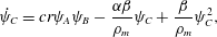 $$\begin{eqnarray}\dot{\unicode[STIX]{x1D713}}_{C}=cr\unicode[STIX]{x1D713}_{A}\unicode[STIX]{x1D713}_{B}-\frac{\unicode[STIX]{x1D6FC}\unicode[STIX]{x1D6FD}}{\unicode[STIX]{x1D70C}_{m}}\unicode[STIX]{x1D713}_{C}+\frac{\unicode[STIX]{x1D6FD}}{\unicode[STIX]{x1D70C}_{m}}\unicode[STIX]{x1D713}_{C}^{2},\end{eqnarray}$$
 where  $\unicode[STIX]{x1D713}_{C}=\unicode[STIX]{x1D713}_{C}(t)$ is the unknown variable and
  $r$,
$r$,  $c$,
$c$,  $\unicode[STIX]{x1D70C}_{m}$,
  $\unicode[STIX]{x1D6FC}$,
  $\unicode[STIX]{x1D6FD}$,
  $\unicode[STIX]{x1D713}_{A}$ and
  $\unicode[STIX]{x1D713}_{B}$ are fixed parameters. Relating this to (A 1), let
  $y=\unicode[STIX]{x1D713}_{C}$,
  $q_{0}=cr\unicode[STIX]{x1D713}_{A}\unicode[STIX]{x1D713}_{B}$,
  $q_{1}=-\unicode[STIX]{x1D6FC}\unicode[STIX]{x1D6FD}/\unicode[STIX]{x1D70C}_{m}$ and
  $q_{2}=\unicode[STIX]{x1D6FD}/\unicode[STIX]{x1D70C}_{m}$. Therefore, in the final equation,
  $R=q_{1}+q_{2}^{\prime }/q_{2}=-\unicode[STIX]{x1D6FC}\unicode[STIX]{x1D6FD}/\unicode[STIX]{x1D70C}_{m}$ and
  $S=q_{0}q_{2}=cr\unicode[STIX]{x1D6FD}\unicode[STIX]{x1D713}_{A}\unicode[STIX]{x1D713}_{B}/\unicode[STIX]{x1D70C}_{m}$.
The solution to (A 5) when  $R$ and
  $S$ are constant depends on the eigenvalues of its corresponding characteristic equation. More specifically, it depends on the sign of the determinant of the root of the characteristic equation
  $R^{2}-4S=\unicode[STIX]{x1D712}/\unicode[STIX]{x1D70C}_{m}^{2}$, where
  $\unicode[STIX]{x1D712}$, defined in § 3.1, was determined to be positive for physically realistic parameter values.
The solution to this case – where the characteristic equation to (A 5) has two real, distinct roots – can be found in any introductory book on ODEs (see Boyce & DiPrima Reference Boyce and DiPrima2008, pp. 137–143), but for completeness the solution is detailed here with homogeneous initial conditions  $y(0)=0$,
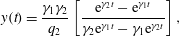 $$\begin{eqnarray}y(t)=\frac{\unicode[STIX]{x1D6FE}_{1}\unicode[STIX]{x1D6FE}_{2}}{q_{2}}\left[\frac{\text{e}^{\unicode[STIX]{x1D6FE}_{2}t}-\text{e}^{\unicode[STIX]{x1D6FE}_{1}t}}{\unicode[STIX]{x1D6FE}_{2}\text{e}^{\unicode[STIX]{x1D6FE}_{1}t}-\unicode[STIX]{x1D6FE}_{1}\text{e}^{\unicode[STIX]{x1D6FE}_{2}t}}\right],\end{eqnarray}$$
where
 $$\begin{eqnarray}\unicode[STIX]{x1D6FE}_{1}=\frac{R+\sqrt{R^{2}-4S}}{2},\quad \unicode[STIX]{x1D6FE}_{2}=\frac{R-\sqrt{R^{2}-4S}}{2},\end{eqnarray}$$
 $$\begin{eqnarray}R=q_{1},\quad S=q_{0}q_{2},\end{eqnarray}$$
and the antiderivative of this solution is given by
 $$\begin{eqnarray}\int y(t)\,\text{d}t=-\frac{1}{q_{2}}\log (\unicode[STIX]{x1D6FE}_{1}\text{e}^{\unicode[STIX]{x1D6FE}_{2}t}-\unicode[STIX]{x1D6FE}_{2}\text{e}^{\unicode[STIX]{x1D6FE}_{1}t})+C,\end{eqnarray}$$
 where  $C$ is an arbitrary constant of integration.


