


1. Introduction
Secondary currents encompass flows that emerge in the cross-stream plane normal to the primary flow direction. Their presence in turbulent flows can result in two different flow patterns in the cross-stream plane: identifiable streamwise vortices and spanwise/cross-flow (Bradshaw Reference Bradshaw1987). The former represent secondary currents of the Prandtl's second kind (Prandtl Reference Prandtl1952), which originate from turbulence anisotropy and spatial gradients of the Reynolds stresses, while the latter is attributed to the presence of a spanwise pressure gradient. In the context of roughness, secondary currents are known to emerge over spanwise inhomogeneous rough surfaces (Hinze Reference Hinze1967), where they are represented by a streamwise aligned pair of vortices separated by high- and low-momentum pathways, i.e. downwash and upwash flow regions. Although secondary current vortices (SCVs) are weak compared with the mean flow, they can introduce significant spanwise heterogeneities to the mean flow field, giving rise to elevated levels of dispersive stresses, which can propagate up to the outer edge of the boundary layer. Therefore, SCVs affect the mean flow and turbulence statistics, as well as influence exchange of momentum and mixing.
Over the last decade, secondary currents over rough surfaces have received significant attention from the fluid mechanics community. Two main classes of rough surfaces have been investigated experimentally and numerically in this context: ridge-type roughness, i.e. surfaces with spanwise variation in topography, and strip-type roughness, which represents surfaces with spanwise variation in skin friction (Wang & Cheng Reference Wang and Cheng2006). For both classes of surfaces, secondary currents were found in the form of SCVs, whose extent primarily depends on the size and spacing of the spanwise surface features. For ridge-type roughness, spanwise spacing between adjacent ridges was identified as a key parameter that governs the size and strength of SCVs (Vanderwel & Ganapathisubramani Reference Vanderwel and Ganapathisubramani2015; Hwang & Lee Reference Hwang and Lee2018; Zampiron, Cameron & Nikora Reference Zampiron, Cameron and Nikora2020). When spacing reaches the outer length scale of the flow, SCVs become space filling and their strength is maximised (Vanderwel & Ganapathisubramani Reference Vanderwel and Ganapathisubramani2015). Other parameters, such as ridge width and shape also have been found to influence the SCVs’ strength (Hwang & Lee Reference Hwang and Lee2018; Medjnoun, Vanderwel & Ganapathisubramani Reference Medjnoun, Vanderwel and Ganapathisubramani2020; Zhdanov, Jelly & Busse Reference Zhdanov, Jelly and Busse2024). However, in all cases reported in the literature the secondary currents materialised in the form of identifiable streamwise vortices, while no presence of net spanwise flow has been reported to date for either ridge-type or strip-type roughness. In the present study, we consider a special class of ridge-type roughness, namely symmetry-breaking streamwise homogeneous surfaces composed of ridges with asymmetric cross-section, which induce not only SCVs but also produce net spanwise flow.
Despite the abundance of literature on secondary currents generated by ridge-type rough surfaces, all previous studies share the same feature, namely the considered ridges have a wall-normal axis of symmetry with respect to the surface on which they are placed. As a result, the secondary current vortices formed in between and/or above ridges are symmetric, i.e. statistically the same differing only in their rotational direction. Compared with other commonly studied cross-sectional geometries, such as rectangular or semicircular ridges, triangular ridges allow for a wider range of modifications to their cross-section. In addition to equilateral and isosceles, triangular ridges can have scalene cross-section with different slopes of their lateral surfaces and therefore break the symmetry of the ridge with respect to the wall-normal direction. For isosceles triangular ridges, we have previously established that narrow ridges, i.e. ridges with higher lateral slopes, produce stronger SCVs compared with wide ridges, i.e. ridges with lower lateral slopes (Zhdanov et al. Reference Zhdanov, Jelly and Busse2024). Since isosceles ridges preserve the symmetry with respect to the wall-normal direction, the vortices in the SCV pair that forms over each ridge are of equal strength and size. As will be shown in the following, scalene ridge cross-sections introduce symmetry-breaking effects due to the imbalance in lateral ridge slopes, significantly alter the SCV topology and induce a net spanwise flow.
The aim of the present study is to systematically investigate the influence of asymmetric ridge cross-section on secondary currents and other effects induced by breaking the left–right symmetry of a ridged surface. To this end, direct numerical simulations of turbulent channel flow are conducted over ridged surfaces with systematically varied degree of cross-sectional asymmetry. In § 2 the numerical methodology is outlined, results are presented and discussed in § 3 and conclusions follow in § 4.
2. Numerical methodology
Direct numerical simulations (DNS) of incompressible fully developed turbulent channel flow over ridge-type rough surfaces are performed using the code iIMB (Busse, Lützner & Sandham Reference Busse, Lützner and Sandham2015). The code has been validated and used in previous studies on surfaces composed of regular roughness elements (e.g. Busse & Zhdanov Reference Busse and Zhdanov2022), including ridge-type roughness that generates secondary currents (Zhdanov et al. Reference Zhdanov, Jelly and Busse2024). The velocity components in the streamwise ( $x$), spanwise ( $\kern0.09em y$) and wall-normal ( $z$) directions are $u$,
$u$,  $v$ and $w$, respectively. The flow is driven by a constant (negative) mean streamwise pressure gradient $\varPi$, which determines the mean friction velocity in the simulation as $u_{\tau }=\sqrt {- \varPi \delta / \rho }$, where $\rho$ is the constant density and $\delta$ is the channel half-height.
A schematic of a channel with ridge-type roughness used for the present DNS is presented in figure 1. The domain has size ( $L_x \times L_y \times L_z$) of $3{\rm \pi} \delta \times {\rm \pi}\delta \times 2\delta$ and is discretised with $1152 \times 576 \times 512$ computational grid points. Spatial resolution is uniform in the streamwise and spanwise directions with $\Delta x^+ = 4.5$ and $\Delta y^+ = 3$. In the wall-normal direction, constant grid spacing is applied up to the ridge crest with $\Delta z^+_{{min}} = 0.67$ and is gradually increased above, reaching a maximum value of $\Delta z^+_{{max}} = 4.69$ at the channel centreplane. The ridges cover both the lower and the upper channel walls which are mirrored with respect to the channel centreplane. The ridge geometry is resolved using an iterative version of the embedded boundary method by Yang & Balaras (Reference Yang and Balaras2006). Periodic boundary conditions are prescribed in the streamwise and spanwise directions, while ridge surfaces are treated as no-slip walls.

Figure 1. Schematic of a channel with ridge-type roughness used for DNS (not to scale). Here,  $\delta$ is the channel half-height, $h$ is the ridge height, $b$ is the ridge base width and $b_1$ and $b_2$ are the left and right ridge base segments. The channel is symmetric with respect to the centreplane and only its lower half is shown.
Four surfaces fully covered with ridges of triangular cross-section are considered. In all cases, ridges have fixed height,  $h/\delta =0.08$, and base width, $b/\delta ={\rm \pi} /4$ (see inset in figure 1). Since the entire channel wall is covered with ridges, the spacing is equivalent to the ridge base width. The ridges with the chosen width/spacing are expected to generate significant secondary currents (Zhdanov et al. Reference Zhdanov, Jelly and Busse2024). The triangular ridge cross-section is systematically varied between cases by changing the ratio of ridge base segments ( $b_1/b_2$), which are obtained by drawing a height to the ridge base. This corresponds to the variation of the ratio between the lateral slopes of the ridge. Starting from an isosceles triangular cross-section ( $b_1/b_2=1$), the symmetry of the cross-section is broken by increasing the ratio of ridge base segments first to 3, then to 7 and finally to $\infty$, which corresponds to the right-angled triangle. Throughout the paper the cases are denoted by using their corresponding ratio $b_1/b_2$ denoted by R followed by the value of R. For instance, the case with ridge base segments ratio of 7 is denoted as R7. Since all cases are streamwise homogeneous, the streamwise effective slope $ES_x$ (Napoli, Armenio & De Marchis Reference Napoli, Armenio and De Marchis2008) is zero in all cases. The spanwise effective slope $ES_y$ (Jelly et al. Reference Jelly, Ramani, Nugroho, Hutchins and Busse2022) is equal to $ES_y=2h/b\approx 0.2037$ for all surfaces, since the ridge height, base width and spacing are constant across all studied cases.
All simulations are conducted at a constant friction Reynolds number of 550, which is defined here as 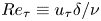 $Re_{\tau } \equiv u_{\tau } \delta / \nu$, where $\nu$ is the kinematic viscosity. In each simulation, flow statistics are acquired for $T u_{\tau }/\delta = 100$ non-dimensional time units after the initial transient, which corresponds to a minimum of 176 flow through times. Statistical quantities are computed using a double-averaged (time-then-space) methodology (Raupach & Shaw Reference Raupach and Shaw1982; Nikora et al. Reference Nikora, McEwan, McLean, Coleman, Pokrajac and Walters2007) together with intrinsic averaging (Gray & Lee Reference Gray and Lee1977), i.e. only the fluid occupied region is considered when computing averages below the ridge crests. In addition, for each simulation 2500 instantaneous three-dimensional snapshots were collected. The snapshots are separated by 22 viscous-scaled time units, $\Delta t^+ \equiv \Delta t u^2_{\tau }/\nu = 22$. The reference smooth-wall DNS is conducted at matched flow conditions, domain size and grid resolution. Throughout the paper, superscript $+$ indicates viscous-scaled quantities, e.g. $v^+ = v/u_{\tau }$, $\overline {{\cdot }}$ denotes time-averaged quantities and $\langle {\cdot } \rangle$ denotes intrinsic averaging over wall-parallel ( $x\unicode{x2013}y$) planes.
3. Results
3.1. Mean flow and global properties
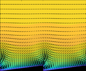
The mean streamwise velocity fields for all four ridged surfaces (R1 to R $\infty$) are presented in figure 2 with superimposed in-plane velocity vectors. As expected from previous studies on turbulent flow over streamwise aligned ridges with symmetric triangular cross-sections (e.g. Stroh et al. Reference Stroh, Schäfer, Forooghi and Frohnapfel2020; Zampiron et al. Reference Zampiron, Cameron and Nikora2020; Zhdanov et al. Reference Zhdanov, Jelly and Busse2024), the present triangular ridges produce SCVs with upwash regions above the ridge crests and downwash over the cavity formed by the lateral surfaces of adjacent ridges accompanied by spanwise heterogeneity of the mean flow field. Isosceles ridges with equal slope of their lateral surfaces (case R1) produce symmetric SCVs with the downwash region aligned with the bottom of the valley between ridges (figure 2a). As the ridge cross-section becomes scalene, the asymmetry in geometry is reflected in the induced secondary current vortices: the vortex formed on the high-slope ridge side is more pronounced compared with its counterpart formed on the low-slope side, and this trend continues as R increases (figure 2b–d). Thus, as expected, an asymmetric ridge cross-section leads to an imbalance in vortices formed over each side of the ridge. The high-slope side vortex suppresses the vortex over the low-slope side and occupies part of the flow above the low-slope side of the ridge. As a result, downwash is not aligned with the bottom of the valley, as in case R1, but occurs over the ridge surface with lower slope.
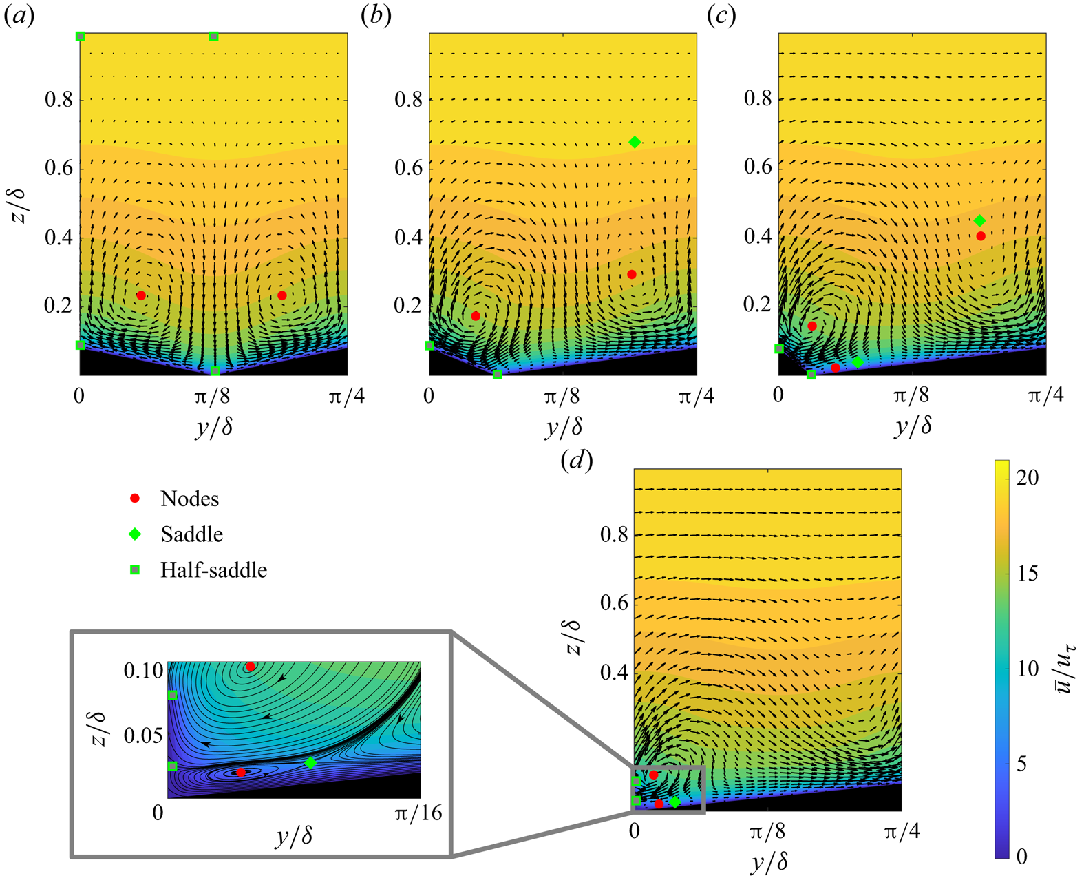
Figure 2. Contours of the phase-averaged mean streamwise velocity with superimposed in-plane velocity vectors (downsampled for clarity): (a) R1, (b) R3, (c) R7, (d) R $\infty$. Locations of critical points in the flow are marked in each panel. For critical points located at the spanwise boundaries only one point is shown.
As is evident from the in-plane velocity vectors, especially in the outer layer, there is a net spanwise flow in the channel for the scalene ridge cases, i.e. scalene ridges produce cross-flow. The net spanwise flow is quantified in figure 3(a), where  $\langle \bar {v} \rangle ^+$ profiles are plotted for all ridge-type cases together with reference smooth-wall data. Before discussing the present results, it should be noted that, for smooth-wall conditions, the mean spanwise velocity is expected to be zero provided that the flow statistics are perfectly converged. However, since in DNS flow statistics are averaged over finite time and domain size, for the present smooth-wall case $\langle \bar {v} \rangle ^+$ is not strictly zero but exhibits small deviations. This is a typical result, as can be seen from the DNS data by Lee & Moser (Reference Lee and Moser2015) for smooth-wall channel flow, which are also plotted in figure 3(a), obtained at the same $Re_{\tau }$ in a much bigger channel ( $L_x \times L_y = 8{\rm \pi} \delta \times 3{\rm \pi} \delta$) but for a shorter time-averaging period. For case R1 (isosceles ridges), $\langle \bar {v} \rangle ^+$ remains close to zero, but, once the ridge cross-section becomes scalene, finite values of spanwise velocity are observed across the channel half-height. In the scalene ridge cases (R3, R7 and R $\infty$) the magnitude of the double-averaged spanwise velocity is higher by a couple of orders of magnitude compared with R1 and the smooth-wall cases. An additional DNS was conducted to verify that scalene ridges generate net spanwise flow using the same set-up as described in § 2. For this simulation, denoted as R7f, the ridged-wall geometry is the same as for case R7 but the ridges are flipped horizontally. As is evident from figure 3(a), case R7f produces net spanwise flow in the opposite direction compared with case R7, while the $\langle \bar {v} \rangle ^+$ magnitude closely matches for both cases. Therefore, the observed net spanwise flow over the scalene ridges is a physical effect and not an artefact of finite averaging.

Figure 3. (a) Double-averaged profiles of spanwise velocity, (b) spanwise velocity at the channel centreplane as a function of the ratio of the wetted areas of the ridge sides.
The spanwise flow direction is not constant across  $z/\delta$: above the ridge crest $\langle \bar {v} \rangle ^+$ has mostly positive values, i.e. the flow direction is away from the high-slope side of the ridge, while below the mean spanwise velocity is largely negative, i.e. the spanwise flow is directed towards the ridge side with high slope. In addition, for cases R7 and R $\infty$ there is a small region at the bottom of the cavity between the ridge sides, which is more pronounced in the latter case, where the spanwise flow direction matches the direction above the crests. This region corresponds to an additional vortex formed under the main SCV in these cases as will be discussed in § 3.2.
Below the ridge crest an increase in R from 3 to 7 has only a minor effect on the spanwise velocity, while further increase to  $\infty$ leads to a drop in $\langle \bar {v} \rangle ^+$ values. Above the ridge crests, the spanwise flow becomes stronger as the ratio between ridge slopes increases with the highest $\langle \bar {v} \rangle ^+$ observed for the case R $\infty$. A peak emerges in the $\langle \bar {v}\rangle ^+$ profiles for the asymmetric ridge cases, which is more pronounced in the R7 and R $\infty$ cases. This peak is located just above the nodal point over the high-slope ridge side (discussed in § 3.2) and corresponds to the lower boundary of the upper sidewash region of the SCV above this ridge side. With respect to the low-slope ridge side the peak location falls within the lower sidewash region of the corresponding secondary current structure (figure 2). Above ridge crest for $z/\delta \gtrapprox 0.5$, the net spanwise velocity approaches a nearly constant value in the outer layer. The spanwise velocity magnitude exhibits an approximately linear correlation with the ratio of the wetted areas of the ridge sides, $A_l/A_h$, where $A_l$ is the wetted area of the low-slope side and $A_h$ is the wetted area of the high-slope side (figure 3b). Although the magnitude of net spanwise flow is low relative to the mean streamwise flow, it is comparable to the vertical velocity in the upwash and downwash regions and spanwise velocity in the sidewash regions of the SCVs. The latter is particularly evident from figures 2(c)–2(d), where the top sidewash region of the SCV generated over the low-slope ridge side is completely suppressed by the spanwise flow, and the mean spanwise flow direction in this region is reversed compared with the case R1, where no spanwise flow is present (figure 2a).
Despite the presence of SCVs and, in the case of asymmetric ridges, net spanwise flow, the studied surfaces exhibit a good level of outer layer similarity, as is evident from the collapse of the streamwise velocity profiles with the smooth-wall data when plotted in defect form (figure 5a). It should be noted that, in our previous study (Zhdanov et al. Reference Zhdanov, Jelly and Busse2024), ridged surfaces with equilateral triangular cross-section with the same spanwise spacing also exhibited a good collapse. The strength of secondary currents is often characterised based on the maximum magnitude of the induced secondary motions compared with the bulk flow velocity  $(\sqrt {\bar {v}^2+\bar {w}^2}/U_b)_{{max}}$ (see, e.g. Stroh et al. Reference Stroh, Schäfer, Forooghi and Frohnapfel2020). A representative example of the magnitude of secondary currents is shown in figure 4(a) for case R7. The strength of secondary currents for each case is shown in figure 4(c). The symmetric ridge case (R1) produces the weakest secondary currents and their maximum magnitude of 1.61 % of $U_b$ is lower compared with 4.4 % found by Medjnoun et al. (Reference Medjnoun, Vanderwel and Ganapathisubramani2020) and Zhdanov et al. (Reference Zhdanov, Jelly and Busse2024) and 6.6 % reported by Stroh et al. (Reference Stroh, Schäfer, Forooghi and Frohnapfel2020). This result is expected, since the ridges in the present study are wider compared with those investigated in the referenced studies and with an increase of ridge base width the strength of secondary currents is known to decrease (see e.g. Hwang & Lee Reference Hwang and Lee2018; Zhdanov et al. Reference Zhdanov, Jelly and Busse2024). In addition, in contrast to previous studies, where the location of maximum magnitude of secondary currents is associated with the upwash regions over ridge crests, for case R1 it is located over the ridge sides. This can be attributed to the full coverage of the channel walls with ridges, while in the referenced studies the ridges were separated by smooth-wall sections, i.e. the ridge base width was smaller than the ridge spacing. An increase in the ridge cross-sectional asymmetry results in progressively higher $(\sqrt {\bar {v}^2+\bar {w}^2}/U_b)_{{max}}$, reaching the highest value for R $\infty$, which exceeds the R1 case by a factor of $1.8$. For the asymmetric cases R3 and R7, the maximum magnitude of secondary currents is found over the high-slope ridge side (see figure 4(a) for R7), while for R $\infty$, where the high-slope side is a vertical wall, it is located in the upwash region above the ridge crest.
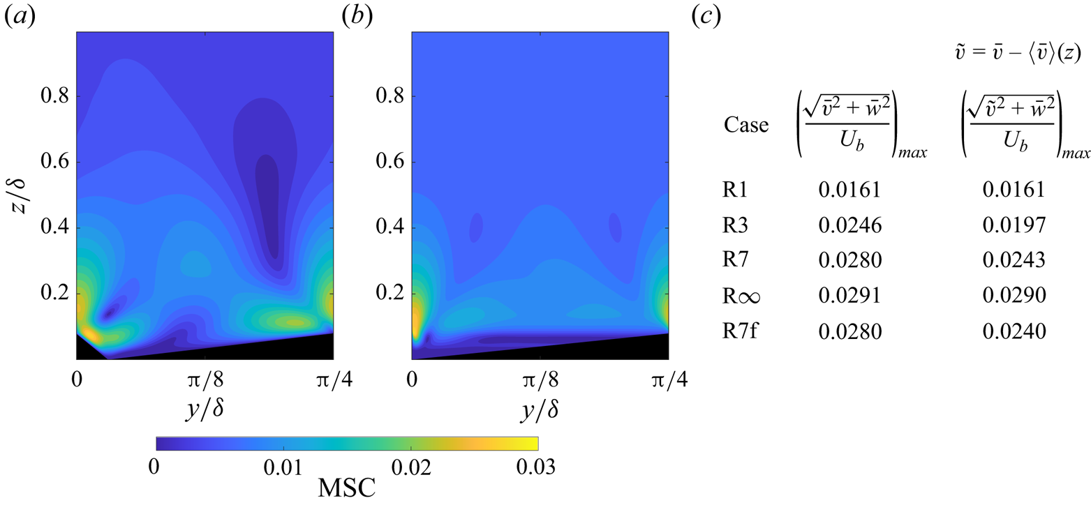
Figure 4. Contours of the phase-averaged magnitude of the secondary currents (MSC) for case R7 (a) with and (b) without net spanwise flow, (c) maximum magnitude of the secondary currents for all studied cases.

Figure 5. Double-averaged profiles of (a) streamwise velocity profiles in defect form, (b) spanwise pressure gradient, (c) sum of in-plane Reynolds and dispersive shear stress  $\langle \overline {v^{\prime }w^{\prime }}\rangle ^+ + \langle \tilde {v} \tilde {w}\rangle ^+$. Reference smooth-wall data are also presented for panels (a,c). The thin vertical dotted line marks location of the ridge crest. (d) Schematic of the spanwise flow induced by surfaces with scalene ridges.
It should be noted that the magnitude of secondary currents grows with the increase in the net spanwise flow, since  $\bar {v}$ is included in its definition. By subtracting the double-averaged spanwise velocity profile from the time-averaged spanwise velocity field it is possible to eliminate the direct contributions of the net spanwise flow (see figure 4b) to the secondary current strength. For cases R3, R7 and R7f subtracting the net spanwise flow for a given wall-normal location results in a reduction of the maximum magnitude of secondary currents (figure 4c) and shifts its location to the region above ridge crest (see figure 4(b) for R7). In contrast, for R $\infty$ no significant change in the maximum secondary current strength is observed, since it is associated with high $\bar {w}$ values in the upwash region.
3.2. Flow topology
The presence of net spanwise flow due to the asymmetric ridge cross-section influences the flow topology, which in the following is analysed through critical points (Hunt et al. Reference Hunt, Abell, Peterka and Woo1978). For each case nodes ( $N$), saddles ( $S$), half-nodes ( $N^{\prime }$) and half-saddles ( $S^{\prime }$) are identified and marked in figure 2. For a singly connected domain, as is the case for the present DNS, the total number of critical points must satisfy the identity (Hunt et al. Reference Hunt, Abell, Peterka and Woo1978)
 \begin{equation} \left(\sum N + \frac{1}{2}\sum N^{\prime}\right) - \left(\sum S + \frac{1}{2}\sum S^{\prime}\right) = 0. \end{equation}
For case R1 there are two nodes located inside each SCV core, two half-saddles in the outer flow at the domain boundaries corresponding to the upwash and downwash regions and two half-saddles on the ridge surface, one at the ridge crest and the second at the bottom of the valley (figure 2a). Overall, the topology resembles typical flow topologies reported earlier for large-scale roughness-induced SCVs above rectangular ridges (Castro et al. Reference Castro, Kim, Stroh and Lim2021) and strip-type roughness (Stroh et al. Reference Stroh, Hasegawa, Kriegseis and Frohnapfel2016). It should be noted that the exact topology depends on the size of the SCVs and the ridge geometry, e.g. for rectangular ridges Castro et al. (Reference Castro, Kim, Stroh and Lim2021) reported a total of 8 half-saddles on the ridge surface and channel wall.
With the emergence of net spanwise flow (case R3), instead of two half-saddles in the outer flow, a single saddle point appears in this region (figure 2b). This critical point is located above the SCV formed on the low-slope ridge side, where the top part of sidewash from this vortex (with  $\bar {v}<0$) is stagnated by the net spanwise flow (with $\bar {v}>0$). The number and location of half-saddles on the ridge surface remains unaffected. Increase in R, and consequent increase in the net spanwise flow magnitude, moves the saddle point in the wall-normal direction closer to the nodal point located inside the secondary current vortex formed on the low-slope ridge side (figure 2c). For case R $\infty$, where the strongest net spanwise flow is observed, these two critical points (node and saddle) above the low-slope ridge side merge (figure 2d). The resultant flow topology in this region corresponds to the case of the merging of two critical points (Moffatt Reference Moffatt2021).
For isosceles triangular ridges the nodal points that correspond to the centres of the secondary current vortices occur at an increasing distance from the wall as the ridge base width is increased (Zhdanov et al. Reference Zhdanov, Jelly and Busse2024). This effect can also be observed for the present scalene triangles: with increasing R, the secondary current centre above the low-slope side moves further away from the wall whereas the corresponding nodal point above the high-slope side moves closer to the wall. As a result, the upper sidewash region of the high-slope ridge side SCV starts to become horizontally aligned with the lower sidewash region of the SCV above the low-slope ridge side, resulting in increasing net positive spanwise flow above the ridge crests as the slope imbalance increases. In addition, as the high-slope side SCV moves closer to the wall its lower sidewash region intensifies and starts to dominate the flow within the cavity, leading to net negative spanwise flow below the ridge crests, as discussed above for the mean spanwise velocity profiles (see figure 3a).
For cases R7 and R $\infty$, an additional vortex, and consequently node, emerges between the ridge surface and the SCV formed over the high-slope ridge side, as can be clearly seen from the inset to figure 2(d), where mean flow streamlines are shown for this part of the domain. The flow topology in this region is very similar in both cases and for brevity is only shown for R $\infty$. In addition, a saddle is formed between this vortex and the downwash part of the flow. The presence of this additional vortex shifts the location of the half-saddle point on the vertical ridge surface to a higher wall-normal location for case R $\infty$, while for R7 this half-saddle remains at the bottom of the valley. In all cases, including those where nodes and saddles merge/appear, the number of critical points in the flow satisfies (3.1).
To summarise, highly asymmetric scalene ridges not only change the location of critical points, but fundamentally alter the topology of the secondary currents due merging of critical points and the emergence of new critical points. Above ridge crests the regions of SCVs with the same sign of  $\bar {v}$ become horizontally aligned, giving rise to net spanwise flow. Alternatively, the observed flow topology for the scalene ridge cases could also be interpreted as the superposition of SCVs with a net spanwise flow. By subtracting the $\langle \bar {v}\rangle ^+$ profiles from the corresponding $\bar {v}^+$ fields, the conventional topology of SCVs can be restored (see figure 4b).
3.3. Decomposition of streamwise vorticity
Further analysis of the observed secondary current patterns can be performed by applying the classification of Bradshaw (Reference Bradshaw1987): SCVs and spanwise flow can be distinguished by the contributions of the spanwise and wall-normal velocity gradient terms to the streamwise vorticity of the mean flow 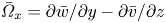 $\bar {\varOmega }_x = \partial \bar {w}/\partial y - \partial \bar {v}/\partial z$. Secondary current vortices are observed in the flow regions where $\partial \bar {v}/\partial z$ and $\partial \bar {w}/\partial y$ have similar magnitude, while spanwise flow occurs where $\partial \bar {v}/\partial z$ makes the dominant contribution to $\bar {\varOmega }_x$. Contours of time- and phase-averaged streamwise vorticity contributions ( $\partial \bar {v}/\partial z$, $\partial \bar {w}/\partial y$) for the present ridged surfaces are shown in figure 6. In all cases the two terms have similar magnitude close to and above the ridge crests, where SCVs are observed for these surfaces. These regions also correspond to the location of non-zero swirl strength (not shown), a quantity which is widely used to characterise SCVs.

Figure 6. Contours of time- and phase-averaged streamwise vorticity components. (a–d)  $\partial \overline {v}^+/ \partial (z/\delta )$, (e–h) $\partial \overline {w}^+/ \partial (y/\delta )$. (a,e) Case R1, (b,f) case R3, (c,g) case R7, (d,h) case R $\infty$.
Within the ridge canopy, the streamwise vorticity is formed predominantly by the  $\partial \bar {v}/\partial z$ term, indicating the presence of spanwise flow, while the sign of $\partial \bar {v}/\partial z$ determines the direction of the local spanwise flow. In the case of ridges with equal side slopes (R1), spanwise flow regions are generated along both ridge sides from the centre of the cavity towards ridge crest (figure 6a). The magnitude of $\partial \bar {v}/\partial z$ closely matches over both sides, amounting to zero net spanwise flow. As the ridge cross-section symmetry is broken (cases R3, R7 and R $\infty$), the spanwise flow still starts close to the midpoint between the two ridge crests in the $y$-direction. However, for scalene ridge cases this location does not correspond to the middle of the cavity as in the isosceles case, and the negative $\partial \bar {v}/\partial z$ region now extends over the low-slope side of the ridge, with the positive $\partial \bar {v}/\partial z$ contours not covering the whole low-slope side (figure 6b–d). As a result, regions of spanwise flow with different directions become imbalanced with stronger flow towards the high-slope ridge side, leading to the observed net spanwise flow within ridge canopy. The maximum difference in $\partial \bar {v}/\partial z$ magnitude increases as the ratio of ridge lateral slopes is changed from 3 to 7 followed by a drop as the ridge cross-section becomes right-angled triangle. This corresponds to the trends observed in the $\langle \bar {v} \rangle ^+$ profiles in the region below the ridge crest (figure 3a).
As discussed in § 3.1, the magnitude of the net spanwise flow within the cavity attains the highest values for the R7 case, whereas the highest net spanwise flow above the ridged surfaces is observed for the right-angled ridge case R $\infty$. Therefore, imbalance in $\partial \bar {v}/\partial z$ regions and hence the spanwise flow within the ridge canopy on its own cannot explain the increase in the net spanwise flow above the ridge crest. The effectiveness of the cavity shape in organising the flow within the cavity needs also to be taken into account. Cavity sides with gradual slopes (as for the present isosceles ridges and low-slope sides of scalene ridges) induce coherent flow parallel to them, which accelerates toward the ridge crest. As the ridge side slope increases (high-slope sides of scalene ridges) part of the spanwise flow is blocked by the ridge surface, with the maximum effect observed in the R $\infty$ case, where the high-slope side is a vertical wall on which a stagnation point forms (see inset to figure 2d). This is also evident in the instantaneous velocity statistics, e.g. in the joint probability density function (j.p.d.f.) of the local spanwise and wall-normal velocity components $P(v,w)$ (see figure 7). Panels (a–d) show the joint p.d.f. for a point close to the high-slope side of the ridge and (e–h) for a point close to the low-slope side. The points are placed at a wall-normal location $z/\delta =0.055$ and at a normal distance $d^+=4.2$ from the ridge surface. Near the left (high-slope) ridge side the j.p.d.f.s are dominated by $Q$2 and $Q$4 events, while close to the right (low-slope) side the dominant contributions come from $Q$1 and $Q$3 events. The shapes of the j.p.d.f.s reflect the changes in flow organisation within the cavity as ridge cross-sectional asymmetry is introduced. For the symmetric ridge case, the j.p.d.f.s for both near-ridge wall locations mirror each other with respect to $v^+=0$ and the most probable events are associated with negative $v^+$ close to the left ridge side and positive $v^+$ close to the right ridge side. As R is increased, the j.p.d.f.s for the high-slope ridge side show a clear change in their orientation with respect to the $v^+$ and $w^+$ axes with an increasing occurrence of high (positive and negative) $w^+$ events and a decrease in high $v^+$ events. For R $\infty$ the shape of the j.p.d.f. becomes more aligned with the $w^+$-axis as more spanwise flow is deflected in the wall-normal direction by the vertical ridge side. In contrast, only very minor changes in the j.p.d.f.s are observed for the location close to the low-slope side of the ridge where the j.p.d.f.s consistently exhibit preferential alignment with the $v^+$-axis. Since secondary currents are uniquely determined by the distribution of the streamwise vorticity of the mean flow (Brundrett & Baines Reference Brundrett and Baines1964; Nikitin, Popelenskaya & Stroh Reference Nikitin, Popelenskaya and Stroh2021), they can be analysed using the transport equation for $\bar {\varOmega }_x$, which for a statistically stationary and streamwise homogeneous flow is given by
 \begin{equation}
\bar{v}\frac{\partial
\bar{\varOmega}_x}{\partial y} + \bar{w} \frac{\partial
\bar{\varOmega}_x}{\partial z} - \nu \left(
\frac{\partial^2 \bar{\varOmega}_x}{\partial y^2} +
\frac{\partial^2 \bar{\varOmega}_x}{\partial z^2} \right)
= S. \end{equation}
\begin{equation}
\bar{v}\frac{\partial
\bar{\varOmega}_x}{\partial y} + \bar{w} \frac{\partial
\bar{\varOmega}_x}{\partial z} - \nu \left(
\frac{\partial^2 \bar{\varOmega}_x}{\partial y^2} +
\frac{\partial^2 \bar{\varOmega}_x}{\partial z^2} \right)
= S. \end{equation}
The first two terms on the left-hand side in (3.2) represent the advection of streamwise mean flow vorticity by the mean flow in the  $y$–
$y$– $z$ plane, while the third term governs its diffusion by viscosity. The source term $S$ on the right-hand side is responsible for production of $\bar {\varOmega }_x$ and consists of spatial gradients of the in-plane Reynolds stresses
 \begin{equation} S =
\underbrace{\frac{\partial^2
\overline{v^{\prime}v^{\prime}}}{\partial y \partial z} -
\frac{\partial^2 \overline{w^{\prime}w^{\prime}}}{\partial y
\partial z}}_{S_1} + \underbrace{\frac{\partial^2
\overline{v^\prime w^\prime}}{\partial z^2} -
\frac{\partial^2 \overline{v^\prime w^\prime}}{\partial
y^2}}_{S_2}.
\end{equation}
\begin{equation} S =
\underbrace{\frac{\partial^2
\overline{v^{\prime}v^{\prime}}}{\partial y \partial z} -
\frac{\partial^2 \overline{w^{\prime}w^{\prime}}}{\partial y
\partial z}}_{S_1} + \underbrace{\frac{\partial^2
\overline{v^\prime w^\prime}}{\partial z^2} -
\frac{\partial^2 \overline{v^\prime w^\prime}}{\partial
y^2}}_{S_2}.
\end{equation}
The contours of the source term for the studied cases are presented in figure 8. As expected from previous studies (e.g. Castro & Kim Reference Castro and Kim2024), the region of the highest vorticity production is located around the ridge crests, which represent a convex corner. For the symmetric ridge case, the regions of positive and negative  $S$ on the left and right ridge sides mirror each other – the source term has largely negative values over the left ridge side and positive values over the right side. As expected, $S^+$ changes its sign at the lines of symmetry (Nikitin et al. Reference Nikitin, Popelenskaya and Stroh2021), i.e. at the centre of the cavity and at the ridge crest. For the scalene ridge cases, these lines of symmetry cease to exist. While the asymmetric ridge cases maintain largely positive values of $S^+$ over the low-slope side which increase in strength with R, the area of negative $S^+$ over the high-slope side shrinks in size and becomes squeezed by an area of positive $S^+$ originating at the ridge crest which tilts clockwise and intensifies as R increases. As a result, regions of positive $S^+$ become dominant above the ridge canopy.
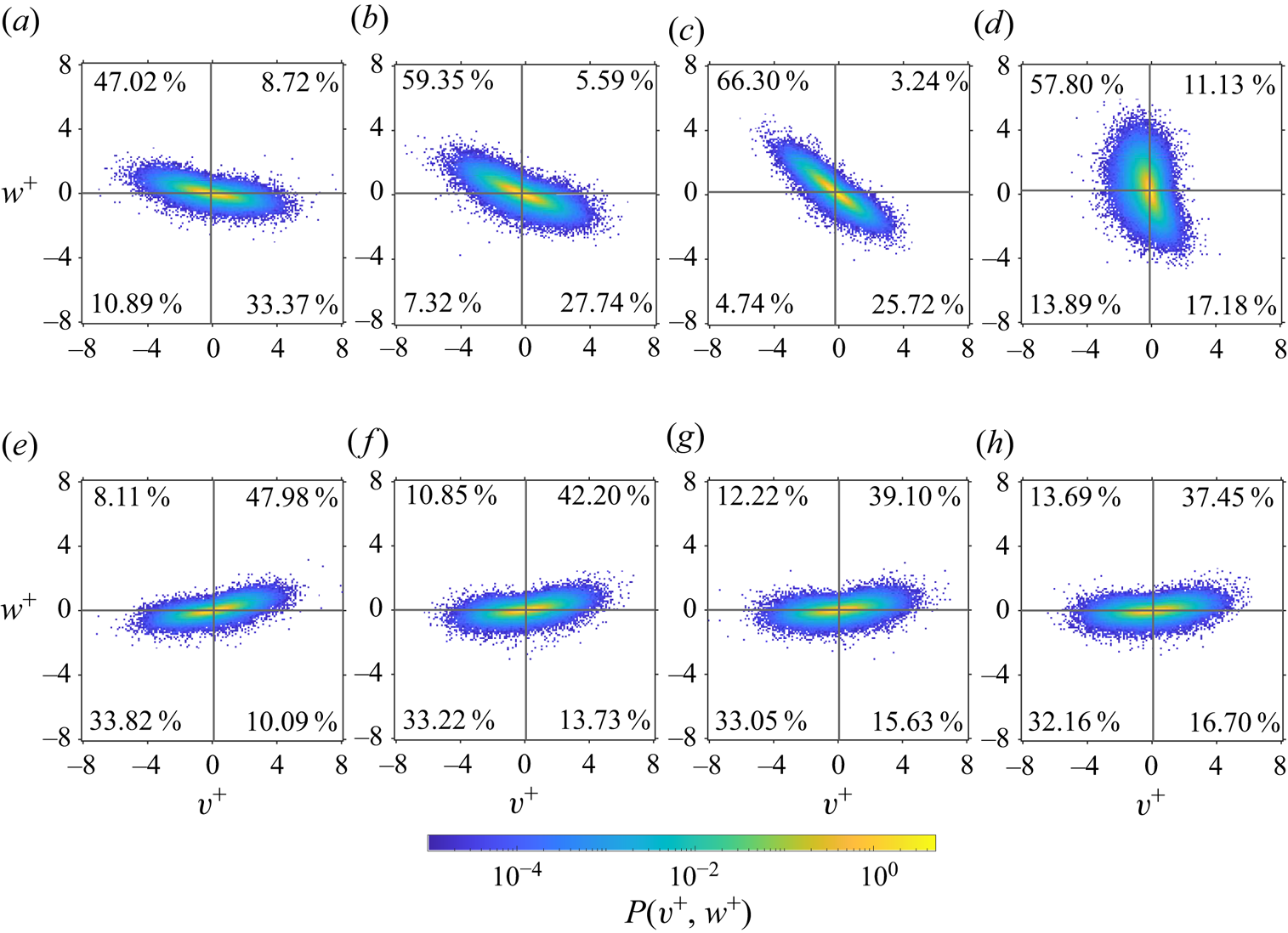
Figure 7. Joint probability density function of the spanwise ( $v^+$) and wall-normal ( $w^+$) velocity components at a wall-normal location $z/\delta =0.055$ and normal distance $d^+= 4.2$ from the ridge wall; (a,e) R1, (b,f) R3, (c,g) R7, (d,h) R $\infty$. The top row (panels a–d) shows joint p.d.f.s close to the high-slope ridge side, bottom row (panels e–h) shows joint p.d.f.s close to the low-slope ridge side. The numbers in each panel show the probability of events in the corresponding quadrant.
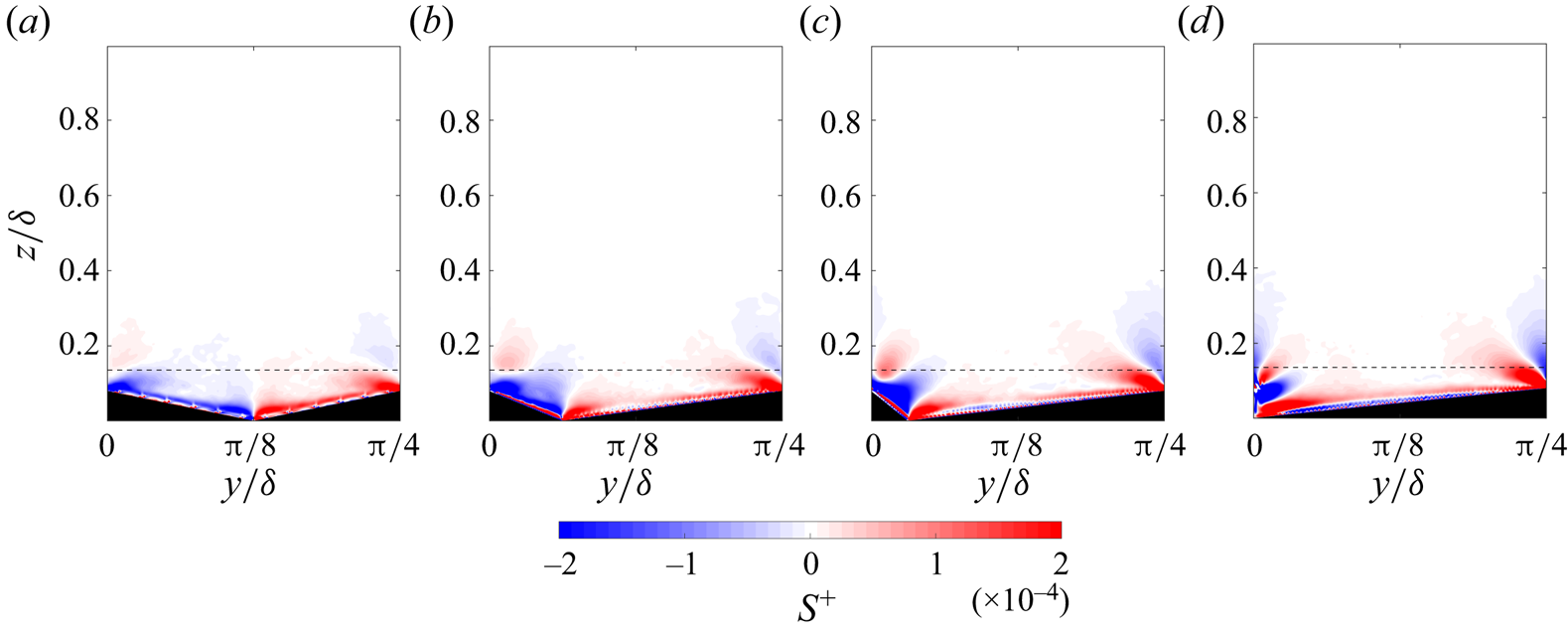
Figure 8. Contours of the source terms of the streamwise vorticity transport equation; (a) R1, (b) R3, (c) R7, (d) R $\infty$. The thin horizontal dashed line in each panel marks the location for which profiles are plotted in figure 9.
This can also be observed from figure 9(a), where the spanwise profiles of the source term are shown for a distance of  ${\approx }30$ wall units above the ridge crest. While for case R1 the $S^+$-profile is approximately point symmetric with respect to the centre of the cavity with a positive maximum over the right slope and a negative minimum over the left slope, the scalene cases show positive local maxima for both sides of the ridge and a negative minimum located close to the ridge crest location. The left maximum can be associated with the upper sidewash region of the SCV over the high-slope ridge side, the right maximum with the lower sidewash region of the SCV over the low-slope ridge side and the minimum with the strong upwash at the ridge crest, which is tilted towards the right for the asymmetric ridge cases.
Figure 9. Spanwise profiles of (a) total source term  $S^+$ in vorticity transport equation at $z^+ \approx 30$ above ridge crest for all cases, (b) two separate terms $S_1^+$ and $S_2^+$ for cases R1 and R $\infty$.
To further explore the change of sign in  $S^+$ over the high-slope ridge side, the spanwise profiles of $S_1^+$ and $S_2^+$ are considered, which for clarity are shown only for R1 and R $\infty$ in figure 9(b). For case R1, $S_1^+$ and $S_2^+$ have similar values but opposite signs and thus production of $\bar {\varOmega }_x$ is largely the result of slightly higher absolute values of $S_2^+$ compared with $S_1^+$. For case R $\infty$, $S_2^+$ still dominates over $S_1^+$, but both $S_1^+$ and $S_2^+$ now take high absolute values at the ridge crest location. Over the high-slope ridge side around the maximum observed for $S^+$ in this case, $S_1^+$ develops a local minimum and $S_2^+$ changes its sign, developing a local maximum. Similar changes can be observed for the other scalene ridge cases.
3.4. Spanwise pressure gradient and net spanwise flow (cross-flow)
In three-dimensional turbulent boundary layers two primary types of spanwise/cross-flow are distinguished based on their origin: pressure driven (e.g. Coleman, Kim & Spalart Reference Coleman, Kim and Spalart2000), i.e. due to imposed spanwise pressure gradient, and shear-driven (e.g. Abe Reference Abe2020), i.e. due to spanwise wall movement. The former also corresponds to Prandtl's secondary currents of the first kind (Bradshaw Reference Bradshaw1987).
In the present DNS, ridged surfaces are treated as stationary no-slip walls and no mean spanwise pressure gradient is applied. While the ridge surfaces are stationary, the imbalance in the SCVs induced by the asymmetric ridges has, from a macroscopic perspective, a similar effect on the mean flow above the ridges as a wall that is slowly moving in the positive  $y$-direction (see schematic shown in figure 5d). Since the ridges on both channel walls mirror each other, the ‘moving-wall effect’ induced by the ridges is in the same direction for both the lower and the upper parts of the channel and thus no Couette-type profile is observed for the mean spanwise velocity component.
Within the scalene ridge canopies, the slope-induced imbalance of the flow over the ridge sides leads to the emergence of a mean spanwise pressure gradient, as can be observed from the double-averaged spanwise pressure gradient  ${\partial \langle \bar {p}\rangle }/{\partial y}$ profiles (figure 5b). While for isosceles ridges the spanwise pressure gradient is close to zero across the whole channel, including the ridge canopy, for scalene ridge cases ${\partial \langle \bar {p}\rangle }/{\partial y}$ has largely non-zero values below the ridge crest. An increase in R leads to higher magnitude of ${\partial \langle \bar {p}\rangle }/{\partial y}$ in this region, which propagates further from the bottom of the valley towards the ridge crest, with high spanwise pressure gradient values observed across almost the entire ridge height in case R $\infty$ (see inset in figure 5b). The resulting flow over the ridges causes a net transfer of spanwise momentum to the flow above the ridges through secondary current vortices and turbulent fluctuations, as can be observed from the corresponding profiles of the sum of in-plane Reynolds $\langle \overline {v^{\prime } w^{\prime }}\rangle ^{+}$ and dispersive shear stress $\langle \tilde {v} \tilde {w}\rangle ^{+}$ (figure 5c), giving rise to the observed net spanwise flow in the channel. The in-plane shear stresses vanish as $z/\delta$ approaches channel half-height as is expected for fully developed wall-shear-driven flow (Howard & Sandham Reference Howard and Sandham2000).
Since the flow above the ridges is not the direct result of a spanwise pressure gradient, the observed cross-flow cannot be classified as secondary current of Prandtl's first kind. Instead, as discussed in the previous sections, the observed net spanwise flow is caused by imbalanced and misaligned secondary currents of Prandtl's second kind. This unusual manifestation of secondary currents may therefore give rise to a new sub-division of secondary currents of the second kind – namely, those with vanishing net spanwise flow, i.e. the type widely reported in the literature for symmetric surfaces, and those where net spanwise flow emerges due to presence of symmetry-breaking effects.
4. Conclusions
Turbulent channel flow over scalene streamwise-aligned ridges has been investigated using DNS. The symmetry-breaking effects of a scalene ridge geometry are evident in the mean flow, where net spanwise flow emerges. The present results show that net spanwise flow can be produced by streamwise homogeneous surfaces due to their geometry, in contrast to previous studies on three-dimensional turbulent boundary layers where cross-flow was introduced by surface shear (moving wall), or the presence of a spanwise pressure gradient, e.g. due to duct curvature or over a swept wing. The magnitude of spanwise flow is directly influenced by the ridge cross-sectional asymmetry, with the maximum  $\langle \bar {v} \rangle ^+$ above the ridge crests induced by the right-angled triangular ridges. Although the spanwise flow is weak compared with the streamwise flow, it has a significant impact on the overall mean flow topology, altering the number and location of critical points compared with the conventional topology of SCVs generated by symmetric ridges or strip-type roughness. The observed net spanwise flow in the scalene ridge cases can be attributed to the increasing alignment between the upper sidewash region of the high-slope SCV with the lower sidewash region of the SCV over the low-slope side as the centre of the high-slope SCV moves closer to the wall and the centre of the SCV over the low-slope side moves further away from the wall with increasing imbalance in the ridge slopes.
The investigated surfaces with asymmetric ridges may have applications for flow control, mixing and drag reduction. It should be noted that scalene triangular cross-section has also been investigated in the context of riblets (Modesti et al. Reference Modesti, Endrikat, Hutchins and Chung2021), which, similarly to ridges, generate SCVs, although of a much smaller size. For right-angled triangular riblets, Modesti et al. (Reference Modesti, Endrikat, Hutchins and Chung2021) reported the presence of spanwise flow regions above and below riblet crests in the same direction as observed for scalene ridges in the present study. However, due to the minimal-channel approach used by Modesti et al. (Reference Modesti, Endrikat, Hutchins and Chung2021) it is not clear whether net spanwise flow extends to the outer layer of the flow as in the present study. For equilateral ridges, the strength of secondary currents intensifies with an increase in Reynolds number (Zhdanov et al. Reference Zhdanov, Jelly and Busse2024), therefore, it would be of interest to determine whether the net spanwise flow is sensitive to this parameter. Finally, it remains to be tested whether the magnitude of the spanwise flow can be increased by optimisation of the surface geometry, e.g. by varying the spanwise effective slope.
Acknowledgements
This work used the ARCHER2 UK National Supercomputing Service (https://www.archer2.ac.uk).
Funding
We gratefully acknowledge support for this work by the United Kingdom's Engineering and Physical Sciences Research Council under grant number EP/V002066/1.
Declaration of interests
The authors report no conflict of interest.
Data availability statement
The data that support the findings of this study are openly available in the University of Glasgow Enlighten repository at http://doi.org/10.5525/gla.researchdata.1680.


 Open access