


1 Introduction
The various approaches for cavitation modelling differ mainly in the treatment of the vapour phase. While Euler–Euler methods assume that liquid and vapour phases are continua, Euler–Lagrange methods consider the vapour phase to be an accumulation of discrete individual bubbles, where only the liquid phase is a continuum. For the continuous phase approach (Euler–Euler), we distinguish between density-based and projection methods. Capturing the phase transition in Euler–Euler methods requires special techniques. Most researchers use a volume of fluid method, where a volume fraction describes the percentage of a phase volume in one control volume. Projection methods solve an additional transport equation for the volume fraction and model vaporisation and condensation using source terms. Simplified cavitation models based on single-bubble dynamics (Rayleigh–Plesset equation) compute these source terms, where vaporisation and condensation depend on the ambient pressure in a control volume. The most common models follow Merkle, Feng & Buelow (Reference Merkle, Feng and Buelow1998), Kunz et al. (Reference Kunz, Boger, Stinebring, Chyczewski, Lindau, Gibeling, Venkateswaran and Govindan2000), Sauer & Schnerr (Reference Sauer and Schnerr2000), Singhal et al. (Reference Singhal, Athavale, Li and Jiang2002) and Zwart, Gerber & Belamri (Reference Zwart, Gerber and Belamri2004).
Euler–Lagrange methods employ a Lagrangian coordinate system to describe the motion of individual cavitation bubbles, which are transported by a continuous liquid background flow. Contrary to Euler–Euler methods, Euler–Lagrange methods consider external forces on the bubble, e.g. forces owing to drag, pressure gradient, volume variation, shear, lift and buoyancy. This leads to relative velocities between the bubbles and the liquid phase and may, therein, cause bubble trajectories to deviate from streamlines of the flow. Equations of bubble dynamics model growth and collapse of every single bubble, see Rayleigh (Reference Rayleigh1917), Plesset (Reference Plesset1949), Tomita & Shima (Reference Tomita and Shima1977) and Hsiao, Chahine & Liu (Reference Hsiao, Chahine and Liu2000). The multiple forces depend on pressure, bubble wall acceleration, surface tension, viscosity and relative velocity between a bubble and the carrier fluid.
Hsiao et al. (Reference Hsiao, Chahine and Liu2000) and Hsiao, Chahine & Liu (Reference Hsiao, Chahine and Liu2003) utilised Lagrangian methods to treat the vapour phase of cavitating flows. Abdel-Maksoud, Hänel & Lantermann (Reference Abdel-Maksoud, Hänel and Lantermann2010) developed a coupled Euler–Lagrange method to calculate cavitating flows. For the flow around a hydrofoil, they compared bubble trajectories and carrier flow streamlines. Their Lagrangian treatment allowed determining of the motion of bubbles relative to the carrier fluid flow. At the outer edge of the foil they examined, these motions deviated significantly from the carrier fluid flow. Yakubov et al. (Reference Yakubov, Cankurt, Maquil, Schiller, Abdel-Maksoud and Rung2011) compared numerical simulations of cavitating flows around a hydrofoil and a propeller using Euler–Euler and Euler–Lagrange approaches. They found a strong dependence of the Euler–Euler simulation on model constants. Using a measured distribution of nuclei, their Euler–Lagrange simulation allowed accounting for water quality effects. Yakubov et al. (Reference Yakubov, Cankurt, Abdel-Maksoud and Rung2013) extended this approach for parallel computing. Ma, Hsiao & Chahine (Reference Ma, Hsiao and Chahine2015a) used an Euler–Lagrange approach to simulate the dynamics of a cavitation cloud consisting of single spherical bubbles. They considered the influence of the liquid phase on the bubbles using a two-way coupled approach. Ma, Hsiao & Chahine (Reference Ma, Hsiao and Chahine2015b) enhanced this approach for parallel simulations.
Pure Euler–Euler approaches to simulate cavitating flows have shown to be efficient and accurate for a wide range of technical flow problems. Disadvantages lie in the prediction of the microscopic cavitation processes of single bubbles. Specifically, to obtain quantitative assessments of cavitation erosion (incubation period, erosion pitting rates, mass loss rates) it is necessary to incorporate the behaviour of single bubbles as they collapse. With Euler–Euler methods the growth and collapse of multiple single bubbles and their motions can only be captured using an extremely fine spatial discretisation. However, the required computational effort is high and, therefore, the microscopic bubble behaviour is usually neglected.
Abdel-Maksoud et al. (Reference Abdel-Maksoud, Hänel and Lantermann2010) showed that, for technical applications, bubble traces may differ significantly from streamlines of the carrier fluid. This is especially true when high pressure and velocity gradients or vortex-induced flows are present. In addition, the predicted cavitation with an Euler–Euler method may show a diffusive behaviour. In the computational domain, this prevents the transport of small amounts of vapour volume fractions and leads to unrealistic results. In this regard, the Euler–Lagrange approach is more accurate because the single bubbles do not vanish owing to an initial non-condensable gas content. However, the computational effort needed to conduct Euler–Lagrange simulations is substantially higher than for Euler–Euler simulations.
To benefit from the efficiency of the Eulerian treatment for the vapour phase and to increase the accuracy of simulating the behaviour of individual single bubbles using a Lagrangian approach, both methods have recently been combined using hybrid multi-scale methods. Depending on the absolute size of a vapour volume and its size relative to the numerical grid, these methods switch between Eulerian and Lagrangian approaches. Accordingly, the dynamics and motions of spherical single bubbles are simulated for small vapour structures, such as collapsing bubbles. Vallier (Reference Vallier2013) developed a multi-scale approach to transform vapour volumes between Eulerian and Lagrangian frames. Using this approach, the author simulated the break up of a cavitation sheet and the cavitation structures on a hydrofoil. Hsiao, Ma & Chahine (Reference Hsiao, Ma and Chahine2017) developed a similar approach to capture the formation of sheet cavitation and shedding of cloud cavitation on a hydrofoil. They used a wall nucleation approach to enable the unsteady shedding of cloud cavitation. Their results agreed favourably with published experimental measurements of sheet cavitation lengths and shedding frequencies. Hsiao, Ma & Chahine (Reference Hsiao, Ma and Chahine2015) used a similar multi-phase approach to simulate sheet and tip vortex cavitation on a three-bladed propeller for three different advance coefficients. They showed that a reduction of the advance coefficient resulted in the extension of sheet cavitation towards the leading edge and the development of tip vortex cavitation caused by single cavitation bubbles merging into a macroscopic cavity. Following their work, Ma, Hsiao & Chahine (Reference Ma, Hsiao and Chahine2017) presented a multi-scale approach to simulate cavitating flow in a waterjet propulsion nozzle, bubbly flow in a line vortex, unsteady sheet cavitation on a hydrofoil and cavitation behind a blunt body. Lidtke (Reference Lidtke2017) used a fully parallel, multi-scale approach to simulate the flow around a hydrofoil to investigate cavitation noise. In contrast to a purely Eulerian approach, the simulation of Lagrangian bubble dynamics enabled the calculation of medium to high frequency pressure fluctuations induced by cavitation. Ghahramani, Arabnejad & Bensow (Reference Ghahramani, Arabnejad and Bensow2018) developed a multi-scale model similar to Vallier (Reference Vallier2013), wherein larger cavities are considered in the Eulerian framework while smaller cavities are treated as Lagrangian bubbles. Although, in contrast to other approaches discussed above (Vallier Reference Vallier2013; Lidtke Reference Lidtke2017; Ma et al. Reference Ma, Hsiao and Chahine2017) their approach transforms small vapour clouds into multiple Lagrangian bubbles and, based on the Eulerian vapour volume fraction, a Lagrangian bubble is introduced into each control volume of a small cavity.
Near-wall collapsing macroscopic cavitation structures, which are accumulations of single cavitation bubbles, cause cavitation-induced erosion. Potentially, these near-wall bubble collapses generate high wall pressures and may cause surface damage, which has been extensively studied both experimentally and numerically. Specifically, collapses of single laser-induced bubbles in undisturbed fields, acoustic fields and near solid boundaries were experimentally studied by Lauterborn & Bolle (Reference Lauterborn and Bolle1975), Vogel & Lauterborn (Reference Vogel and Lauterborn1988), Noack & Vogel (Reference Noack and Vogel1998), Philipp & Lauterborn (Reference Philipp and Lauterborn1998), Brujan et al. (Reference Brujan, Keen, Vogel and Blake2002), Lauterborn & Kurz (Reference Lauterborn and Kurz2010), Lauterborn & Vogel (Reference Lauterborn and Vogel2013), Reuter & Mettin (Reference Reuter and Mettin2016), Reuter, Cairós & Mettin (Reference Reuter, Cairós and Mettin2016), Supponen et al. (Reference Supponen, Obreschkow, Tinguely, Kobel, Dorsaz and Farhat2016), Dular et al. (Reference Dular, Požar, Zevnik and Petkovšek2019), Sagar et al. (Reference Sagar, Hanke, Underberg, Feng, el Moctar and Kaiser2018), Sagar (Reference Sagar2018) and Sagar & el Moctar (Reference Sagar and el Moctar2020). Numerical simulations of near-wall single bubble collapses were conducted by Johnsen & Colonius (Reference Johnsen and Colonius2008, Reference Johnsen and Colonius2009), Osterman, Dular & Širok (Reference Osterman, Dular and Širok2009), Hawker & Ventikos (Reference Hawker and Ventikos2012), Lauer et al. (Reference Lauer, Hu, Hickel and Adams2012), Chahine & Hsiao (Reference Chahine and Hsiao2015), Pöhl et al. (Reference Pöhl, Mottyll, Skoda and Huth2015), Koch et al. (Reference Koch, Lechner, Reuter, Köhler, Mettin and Lauterborn2016), Goncalves et al. (Reference Goncalves, Zeidan, Goncalves and Zeidan2017) and Hadlabdaoui et al. (Reference Hadlabdaoui, Parnaudeau, Goncalves and Zeidan2019).
Over the past years, several researchers have developed numerical approaches to assess cavitation erosion. These approaches rely on different assumptions of the physical processes involved and use various numerical techniques to simulate cavitation behaviour. Assuming that the collapse of cloud cavitation is the main cause of cavitation erosion, Li (Reference Li2012) developed a numerical model using the time derivative of pressure on a surface to indicate erosion risk. When a threshold of the time derivative of pressure is exceeded on a given surface, this region is identified with a high risk of erosion. However, the threshold value must be calibrated for each flow problem. Furthermore, the Euler–Euler method does not allow accurate predictions of the bubble behaviour and collapse-induced pressures in a cloud of bubbles or in regions close to a solid surface. Krumenacker, Fortes-Patella & Archer (Reference Krumenacker, Fortes-Patella and Archer2014) developed a numerical method that determines the cavitation intensity as an indicator for erosion risk when cloud-like cavitation areas collapse. In their method, the flow is simulated using an Euler–Euler approach and a Reynolds-averaged Navier–Stokes (RANS) method coupled with a solver to compute the acoustic energy of single bubbles from a bubble dynamics equation. Accumulation of the acoustic energy of all collapsing single bubbles then yields the cavitation intensity on a given surface. Accounting for bubble dynamics in the erosion model improves the assessment of erosion. Mottyll (Reference Mottyll2017) used a density-based solver to simulate cavitation and evaluated erosion using a collapse detection approach. The author assumes that aggressive types of cavitation are related to collapsing cavitation volumes in the vicinity of solid walls. The model was applied to an axisymmetric nozzle and an ultrasonic horn and obtained qualitatively favourable agreement. When a single cavitation bubble collapses near a solid surface, the collapse is asymmetric causing a high-speed waterjet to flow through the vapour-filled bubble. Dular, Stoffel & Širok (Reference Dular, Stoffel and Širok2006) and Dular & Coutier-Delgosha (Reference Dular and Coutier-Delgosha2009) developed a numerical erosion model by assuming that this microjet is the main cause of erosion leading to circular pits. For a foil in two-dimensional flow the quality of their erosion assessments compared favourably to experiments. Peters, Lantermann & el Moctar (Reference Peters, Lantermann and el Moctar2015a), Peters et al. (Reference Peters, Sagar, Lantermann and el Moctar2015b) expanded the models of Dular et al. (Reference Dular, Stoffel and Širok2006) and Dular & Coutier-Delgosha (Reference Dular and Coutier-Delgosha2009) and validated their results against experiments for a three-dimensional flow case. The qualitative assessment of erosion considered both number and intensity of microjet impacts on an area. Peters, Lantermann & el Moctar (Reference Peters, Lantermann and el Moctar2018) used a similar erosion model to estimate cavitation erosion for a model propeller. Although their erosion assessments agreed with experimental erosion predictions for different flow problems, we found that an Euler–Euler approach provides only a qualitative estimation of erosion. For a more accurate assessment of erosion caused by collapsing cavitation bubbles near a solid surface, detailed insight into the transport and the dynamics of bubbles is needed.
The existing approaches and models to simulate cavitating flows and to assess erosion led us to develop a method that couples an Euler–Euler method with an Euler–Lagrange method. Based on existing libraries, we implemented the new method into the open source computational fluid dynamics (CFD) software package OpenFOAM (OpenFOAM Foundation 2018) that combines the Lagrangian tracking of bubbles with a finite volume method flow solver. Our approach enabled a more accurate assessment of erosion and the potential to assess damage rates. The computation of transport and dynamics of spherical single bubbles provided greater insight into bubble behaviour. Depending on their absolute size and spatial resolution relative to the numerical grid, our multi-scale approach switched between an Eulerian and a Lagrangian treatment of vapour structures. Accordingly, Eulerian vapour volumes were transformed into Lagrangian bubbles when the vapour volumes were isolated and sufficiently small. Motions and dynamics of spherical Lagrangian bubbles were solved individually. Lagrangian bubbles that increased above a certain size or that were sufficiently resolved by the numerical grid were transformed into Eulerian vapour volumes. The assessment of cavitation erosion was based on the information about collapses of Lagrangian bubbles near a solid surface. A comparison of spherical bubble collapses and pit erosion presented here provided insights for a quantitative estimate of erosion by correlating spherical bubble collapses with experimentally measured erosion pits.
Our numerical methods for continuous flows and for Lagrangian bubbles include a procedure to transform vapour volumes between the Eulerian and the Lagrangian frames. Based on nuclei measurements, a distribution of the initial gas content in Lagrangian bubbles is derived. An erosion model based on an Eulerian treatment of the vapour phase is described, and a new erosion model based on Lagrangian bubble collapses is developed. Our multi-scale approach links the macroscopic Eulerian treatment of large vapour structures to the microscopic Lagrangian treatment of single cavitation bubbles and uses the bubble collapses to assess cavitation-induced erosion. After verifying and validating our bubble dynamics model for different cases, we performed verification and sensitivity studies related to the procedures to transform vapour volumes between these frames. The cavitating flow through an axisymmetric nozzle was simulated, and numerically evaluated cavitation-induced erosion was compared to measured erosion depths.
2 Multi-scale approach to assess cavitation erosion
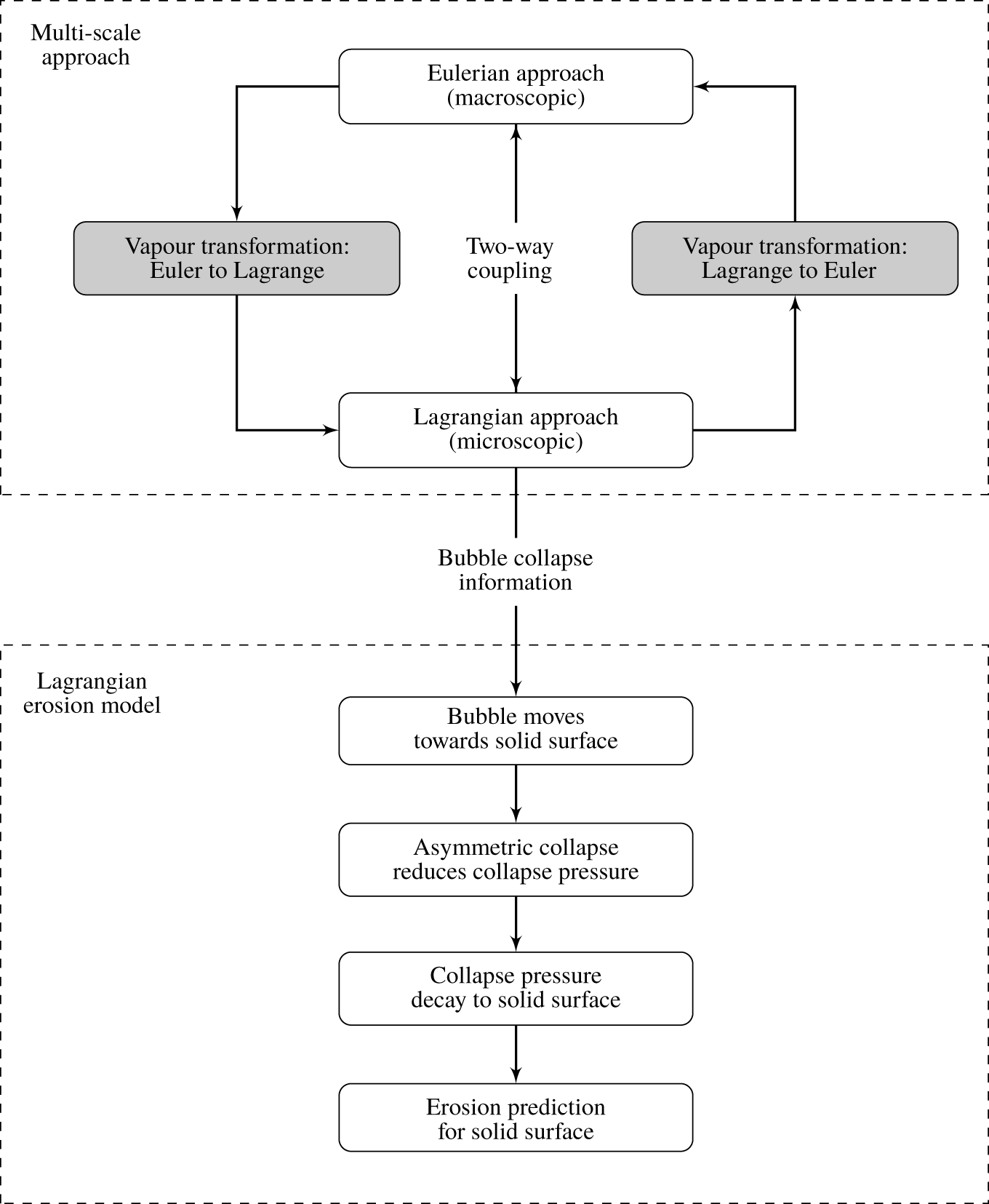
Figure 1. Schematic of the coupling of the multi-scale method with the Lagrangian erosion model.
This section summarises our approach based on a multi-scale treatment of cavitation structures and a model to assess erosion from Lagrangian bubble collapses. Figure 1 schematically depicts the multi-scale method to simulate cavitation and its coupling with the Lagrangian erosion model. The multi-scale method treats the liquid phase as a continuum in the Eulerian frame, but uses different approaches for vapour volumes. Large vapour structures are treated also in the Eulerian frame, while small vapour volumes are considered as spherical Lagrangian bubbles, whose motions and associated bubble dynamics are calculated on a local coordinate system. While fully conserving the volume of vapour, vapour structures are transformed between the Eulerian and the Lagrangian frame and vice versa when they fall below or exceed a defined absolute size or the size relative to the numerical grid. Lagrangian bubbles interact with the continuous liquid phase via a two-way coupling scheme that accounts for influences of the liquid phase on the Lagrangian bubbles and contrariwise. Information from Lagrangian bubble collapses near solid surfaces (e.g. pressures, positions, radii) serve to estimate erosion. Resolving shock wave radiation for asymmetric bubble collapses in a macroscopic flow simulation was almost impossible because, at this moment, the computational effort would have been too high. Therefore, we chose to model the physics involved in an asymmetric near-wall bubble collapse based on well-recognised fundamental experiments and theoretical considerations. The erosion model accounts for various phenomena during an asymmetric bubble collapse, such as (i) the motion of the bubble’s centre towards the solid surface, (ii) the reduced collapse pressure attributed to the non-spherical collapse and (iii) the pressure decay of the shock wave that travels towards the solid surface.
Figure 2 sketches the approaches used for the different physical phenomena involved in the process of cavitation erosion. The multi-scale method creates a link between large vapour structures that are treated in the Eulerian frame and small Lagrangian vapour bubbles. The erosion model links the dynamics of single Lagrangian bubbles near a solid surface to the assessment of erosion and accounts for various phenomena involved in an asymmetric near-wall bubble collapse.
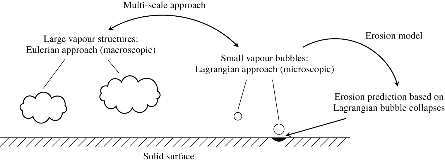
Figure 2. Sketch of approaches used for various cavitation regimes and for erosion evaluation.
3 Numerical method
Cavitation of macroscopic vapour structures is simulated using an Euler–Euler approach that considers the liquid and vapour phases as continua. Microscopic vapour structures are treated as single Lagrangian bubbles transported by the continuous carrier fluid flow. Numerical approaches for Eulerian and Lagrangian approaches are given in the following.
3.1 Continuous Eulerian phases
A homogeneous mixture approach simulates the macroscopic cavitating flow on an Eulerian grid. Substance properties of liquid and vapour phases vary according to the volume fraction of each phase in the mixture. The vapour volume fraction is defined as  $\unicode[STIX]{x1D6FC}_{v}=V_{v}/V$ with the volume of vapour, $V_{v}$, in a certain control volume, $V$. For a two phase flow, the liquid volume fraction is defined as $\unicode[STIX]{x1D6FC}_{l}=1-\unicode[STIX]{x1D6FC}_{v}$. Using the volume fraction variables, the density, $\unicode[STIX]{x1D70C}$, and viscosity, $\unicode[STIX]{x1D707}$, of the mixture can be calculated
 $$\begin{eqnarray}\unicode[STIX]{x1D70C}=\unicode[STIX]{x1D6FC}_{v}\unicode[STIX]{x1D70C}_{v}+(1-\unicode[STIX]{x1D6FC}_{v})\unicode[STIX]{x1D70C}_{l},\quad \unicode[STIX]{x1D707}=\unicode[STIX]{x1D6FC}_{v}\unicode[STIX]{x1D707}_{v}+(1-\unicode[STIX]{x1D6FC}_{v})\unicode[STIX]{x1D707}_{l}.\end{eqnarray}$$
 Indices ‘ $v$’ denote properties of the vapour phase; indices ‘ $l$’, properties of the liquid phase. Properties of the mixture are then used to calculate the flow properties for the mixture fluid.
The continuous flow of the homogeneous mixture is calculated based on the mass conservation equation and the Navier–Stokes equations for an isothermal fluid consisting of the equations of conservation of momentum. The equations for the present finite volume method are written in integral form. The mass conservation equation yields
 $$\begin{eqnarray}\frac{\unicode[STIX]{x2202}}{\unicode[STIX]{x2202}t}\int _{V}\unicode[STIX]{x1D70C}\,\text{d}V+\int _{S}\unicode[STIX]{x1D70C}\boldsymbol{u}\boldsymbol{\cdot }\text{d}\boldsymbol{S}=0,\end{eqnarray}$$
 where  $t$ is time, $V$ is the volume of a control volume, $\boldsymbol{S}$ is the surface area vector of a control volume’s surface and $\boldsymbol{u}$ is the flow velocity of the mixture. The velocity is calculated from the momentum equation
 $$\begin{eqnarray}\displaystyle \frac{\unicode[STIX]{x2202}}{\unicode[STIX]{x2202}t}\int _{V}\unicode[STIX]{x1D70C}\boldsymbol{u}\,\text{d}V+\int _{S}\unicode[STIX]{x1D70C}\boldsymbol{u}\boldsymbol{u}\boldsymbol{\cdot }\text{d}\boldsymbol{S} & = & \displaystyle \int _{S}\unicode[STIX]{x1D707}(\unicode[STIX]{x1D735}\boldsymbol{u}+(\unicode[STIX]{x1D735}\boldsymbol{u})^{\text{T}})\boldsymbol{\cdot }\text{d}\boldsymbol{S}-\int _{S}\left(p-\frac{2}{3}\unicode[STIX]{x1D735}\boldsymbol{\cdot }\unicode[STIX]{x1D707}\right)\unicode[STIX]{x1D644}\boldsymbol{\cdot }\text{d}\boldsymbol{S}\nonumber\\ \displaystyle & & \displaystyle +\,\int _{V}\unicode[STIX]{x1D70C}\boldsymbol{b}\,\text{d}V+\int _{V}\unicode[STIX]{x1D70E}\unicode[STIX]{x1D705}\unicode[STIX]{x1D735}\unicode[STIX]{x1D6FC}\,\text{d}V+\int _{V}\boldsymbol{s}_{b}\,\text{d}V,\end{eqnarray}$$
 where  $\unicode[STIX]{x1D707}$ is viscosity of the mixture, $p$ is pressure and $\unicode[STIX]{x1D644}$ is the identity matrix. The left-hand side comprises the time derivative of momentum and the convection term. The first two terms on the right-hand side represent diffusion and pressure, respectively. Symbol $\boldsymbol{b}$ stands for sources of volume forces caused by gravity or Coriolis effects. The last term on the right-hand side contains the source term originating from Lagrangian bubbles entering a control volume, $\boldsymbol{s}_{b}$. The second to last term on the right-hand side accounts for forces owing to surface tension, $\unicode[STIX]{x1D70E}$, between liquid and vapour phases treated in the Eulerian framework, where $\unicode[STIX]{x1D705}$ is the curvature of the interface. As surface tension acts directly at the interface between the two phases, it cannot explicitly be applied in interface capturing methods, where the interface is smeared over multiple control volumes. We used the continuum surface model, introduced by Brackbill, Kothe & Zemach (Reference Brackbill, Kothe and Zemach1992), to calculate the surface tension force as a volume force acting on the control volume. The curvature of the interface is defined as follows:
 $$\begin{eqnarray}\unicode[STIX]{x1D705}=-\unicode[STIX]{x1D735}\boldsymbol{\cdot }\frac{\unicode[STIX]{x1D735}\unicode[STIX]{x1D6FC}}{|\unicode[STIX]{x1D735}\unicode[STIX]{x1D6FC}|},\end{eqnarray}$$
 where the gradient of the volume fraction,  $\unicode[STIX]{x1D735}\unicode[STIX]{x1D6FC}$, points into the normal direction of the interface. Surface tension vanishes in control volumes occupying only one phase ( $\unicode[STIX]{x1D735}\unicode[STIX]{x1D6FC}=0$).
The system of equations contains the momentum equation to calculate velocities. The continuity equation does not serve for the calculation of pressure because it does not contain the pressure. To close this system of equations, an additional equation for the pressure is derived. First, the mass conservation equation is rearranged. Using Gauss’ theorem to convert a surface integral into a volume integral and letting the arbitrary volume become zero, equation (3.2) is written in differential form. Following Shams, Finn & Apte (Reference Shams, Finn and Apte2010) and rearranging terms leads to the following expression:
 $$\begin{eqnarray}\unicode[STIX]{x1D735}\boldsymbol{\cdot }\boldsymbol{u}=-\frac{1}{\unicode[STIX]{x1D70C}}\frac{\text{d}\unicode[STIX]{x1D70C}}{\text{d}t}.\end{eqnarray}$$
For an incompressible isothermal single phase flow, the density along the path of a fluid particle does not change. This leads to a divergence free velocity field, causing the term on the right-hand side of (3.5) to vanish. However, for cavitating flows, the changing density of the moving free surface and the vaporisation and condensation processes must be considered. The density varies and, therefore, the velocity field diverges. Integrating over a control volume and applying Gauss’ theorem yields the following integral equation:
 $$\begin{eqnarray}\int _{S}\boldsymbol{u}\boldsymbol{\cdot }\text{d}\boldsymbol{S}=-\int _{V}\frac{1}{\unicode[STIX]{x1D70C}}\frac{\text{d}\unicode[STIX]{x1D70C}}{\text{d}t}\,\text{d}V.\end{eqnarray}$$
The partially discretised form of the momentum equation according to Jasak (Reference Jasak1996) is used to obtain the equation containing the pressure
 $$\begin{eqnarray}a_{P}\boldsymbol{u}_{P}=-\mathop{\sum }_{N}a_{N}\boldsymbol{u}_{N}+\boldsymbol{S}_{u}(\boldsymbol{x},t)+\unicode[STIX]{x1D735}p=\boldsymbol{H}(\boldsymbol{u})-\unicode[STIX]{x1D735}p,\end{eqnarray}$$
 where  $a$ are matrix coefficients for the linear system of equations. Indices $P$ and $N$ identify the considered control volume (cell) and the neighbouring control volumes, respectively, and $\boldsymbol{S}_{u}$ is a known source vector for all cells. Accordingly, $\boldsymbol{H}(\boldsymbol{u})$ contains the velocity terms from neighbouring cells, $(-\sum _{N}a_{N}\boldsymbol{u}_{N})$, including all source terms which do not depend on pressure, $\boldsymbol{S}_{u}$. Dividing (3.7) by $a_{P}$ yields the following relationship:
 $$\begin{eqnarray}\boldsymbol{u}_{P}=\frac{\boldsymbol{H}(\boldsymbol{u})}{a_{P}}-\frac{\unicode[STIX]{x1D735}p}{a_{P}}.\end{eqnarray}$$
 Substituting (3.8) into (3.5) for cell index  $P$ we obtain the Poisson equation
 $$\begin{eqnarray}\unicode[STIX]{x1D735}\boldsymbol{\cdot }\left(\frac{\boldsymbol{H}(\boldsymbol{u})}{a_{P}}\right)-\unicode[STIX]{x1D735}\boldsymbol{\cdot }\left(\frac{\unicode[STIX]{x1D735}p}{a_{P}}\right)=-\frac{1}{\unicode[STIX]{x1D70C}}\frac{\text{d}\unicode[STIX]{x1D70C}}{\text{d}t}.\end{eqnarray}$$
 The term on the right-hand side vanishes only in regions where no vaporisation and condensation or transport of a free surface take place. According to Sauer (Reference Sauer2000), the right-hand side can be expressed using source terms from the cavitation model for vaporisation,  $S_{pv}$, and condensation, $S_{pc}$, multiplied by the pressure difference between local fluid pressure, $p$, and vapour pressure, $p_{v}$, as follows:
 $$\begin{eqnarray}\unicode[STIX]{x1D735}\boldsymbol{\cdot }\left(\frac{\boldsymbol{H}(\boldsymbol{u})}{a_{P}}\right)-\unicode[STIX]{x1D735}\boldsymbol{\cdot }\left(\frac{\unicode[STIX]{x1D735}p}{a_{P}}\right)=(S_{p,c}-S_{p,v})(p-p_{v}).\end{eqnarray}$$
 We separate the hydrostatic part from the absolute pressure, where  $p_{rgh}=p-\unicode[STIX]{x1D70C}g_{z}h$. $g_{z}$ is the vertical component of the vector of gravitational acceleration, and $h$ is the height of the water column. Separating the hydrostatic part from the absolute pressure enables us to treat implicitly all terms proportional to $p_{rgh}$. After rearranging terms in (3.10) and separating the pressures, the pressure equation is written as follows:
 $$\begin{eqnarray}\unicode[STIX]{x1D735}\boldsymbol{\cdot }\left(\frac{\unicode[STIX]{x1D735}p_{rgh}}{a_{P}}\right)+(S_{p,c}-S_{p,v})p_{rgh}=\unicode[STIX]{x1D735}\boldsymbol{\cdot }\left(\frac{\boldsymbol{H}(\boldsymbol{u})}{a_{P}}\right)+(S_{p,c}-S_{p,v})(p_{v}-\unicode[STIX]{x1D70C}g_{z}h).\end{eqnarray}$$
 Terms on the left-hand side are treated implicitly; terms on the right-hand side, explicitly. Substituting the temporal derivative of density in (3.9) by terms proportional to  $p_{rgh}$ increases the stability of the equation. The source terms on the right-hand side are treated explicitly and have to be calculated in advance. These source terms depend on space and time and are obtained from a cavitation model representing the processes of vaporisation (‘ $v$’) and condensation (‘ $c$’). Applying the cavitation model of Sauer & Schnerr (Reference Sauer and Schnerr2000) that assumes both continuous phases to be incompressible we obtain the volume of vapour in a considered control volume via the solution of a scalar transport equation
 $$\begin{eqnarray}\frac{\unicode[STIX]{x2202}}{\unicode[STIX]{x2202}t}\int _{V}\unicode[STIX]{x1D6FC}_{v}\,\text{d}V+\int _{S}\unicode[STIX]{x1D6FC}_{v}\boldsymbol{u}\boldsymbol{\cdot }\text{d}\boldsymbol{S}=\int _{V}(S_{v}-S_{c})\,\text{d}V.\end{eqnarray}$$
 Derivation of the cavitation source terms,  $S_{v}$ and $S_{c}$, on the right-hand side is based on a simplified Rayleigh–Plesset equation, which defines the velocity of the bubble wall, $\text{d}R/\text{d}t$, for a bubble of radius $R$. For a positive velocity of the bubble wall, we speak of the bubble growth rate that is calculated from a simplified Rayleigh–Plesset equation as follows:
 $$\begin{eqnarray}\frac{\text{d}R}{\text{d}t}=\sqrt{\frac{2(p_{v}-p)}{3\unicode[STIX]{x1D70C}_{l}}},\quad \text{if }p<p_{v}.\end{eqnarray}$$
On the other hand, the negative velocity of the bubble wall, referred to as bubble collapse rate, is calculated as follows:
 $$\begin{eqnarray}\frac{\text{d}R}{\text{d}t}=\sqrt{\frac{2(p-p_{v})}{3\unicode[STIX]{x1D70C}_{l}}},\quad \text{if }p\geqslant p_{v}.\end{eqnarray}$$
This assumption is rough because it neglects influences attributable to bubble radius acceleration, non-condensable gas, viscosity and surface tension in the Rayleigh–Plesset equation (3.36). Moreover, the change of sign under the root from (3.13) to (3.14) cannot be accounted for by the pressure term in the Rayleigh–Plesset equation. In the cavitation model of Sauer & Schnerr (Reference Sauer and Schnerr2000), the source terms are derived from the continuity equation using the homogeneous mixture expressions of density and assuming a homogeneous distribution of cavitation nuclei per volume of liquid. The source terms depend on the aforementioned simplified calculations of the bubble growth rate as follows:
 $$\begin{eqnarray}\displaystyle \left.\begin{array}{@{}c@{}}\!\!\displaystyle S_{v}=\left\{\begin{array}{@{}l@{}}\displaystyle (-C_{v})\frac{1}{R(\unicode[STIX]{x1D6FC}_{l})}\left[\frac{1}{\unicode[STIX]{x1D70C}_{l}}-\unicode[STIX]{x1D6FC}_{l}\left(\frac{1}{\unicode[STIX]{x1D70C}_{l}}-\frac{1}{\unicode[STIX]{x1D70C}_{v}}\right)\right]\frac{3\unicode[STIX]{x1D70C}_{v}\unicode[STIX]{x1D70C}_{l}}{\unicode[STIX]{x1D70C}}(1+\unicode[STIX]{x1D6FC}_{nuc}-\unicode[STIX]{x1D6FC}_{l})\sqrt{\frac{2}{3}\frac{p_{v}-p}{\unicode[STIX]{x1D70C}_{l}}},\quad \text{if }p<p_{v}\quad \\ 0\quad \text{else},\quad \end{array}\right.\\ \displaystyle S_{c}=\left\{\begin{array}{@{}l@{}}\displaystyle C_{c}\frac{1}{R(\unicode[STIX]{x1D6FC}_{l})}\left[\frac{1}{\unicode[STIX]{x1D70C}_{l}}-\unicode[STIX]{x1D6FC}_{l}\left(\frac{1}{\unicode[STIX]{x1D70C}_{l}}-\frac{1}{\unicode[STIX]{x1D70C}_{v}}\right)\right]\frac{3\unicode[STIX]{x1D70C}_{v}\unicode[STIX]{x1D70C}_{l}}{\unicode[STIX]{x1D70C}}\unicode[STIX]{x1D6FC}_{l}\sqrt{\frac{2}{3}\frac{p-p_{v}}{\unicode[STIX]{x1D70C}_{l}}},\quad \text{if }p\geqslant p_{v}\quad \\ 0\quad \text{else},\quad \end{array}\right.\end{array}\!\!\!\!\!\!\right\} & & \displaystyle \nonumber\\ \displaystyle & & \displaystyle\end{eqnarray}$$
 where  $\unicode[STIX]{x1D6FC}_{l}$ is the liquid volume fraction, $\unicode[STIX]{x1D6FC}_{nuc}$ is the volume fraction owing to the presence of initial gas nuclei and $R(\unicode[STIX]{x1D6FC}_{l})$ is the bubble radius as a function of $\unicode[STIX]{x1D6FC}_{l}$. The constants of vaporisation, $C_{v}$, and of condensation, $C_{c}$, are set to unity. The bubble radius is calculated as follows:
 $$\begin{eqnarray}R(\unicode[STIX]{x1D6FC}_{l})=\sqrt[3]{\frac{3(1-\unicode[STIX]{x1D6FC}_{l}+\unicode[STIX]{x1D6FC}_{nuc})}{\unicode[STIX]{x1D6FC}_{l}4\unicode[STIX]{x03C0}n_{b}}},\end{eqnarray}$$
 where  $n_{b}$ is the nucleus density which defines the number of bubbles per volume of liquid. The reciprocal bubble radius can be written as follows:
 $$\begin{eqnarray}\frac{1}{R(\unicode[STIX]{x1D6FC}_{l})}=\left(\frac{4\unicode[STIX]{x03C0}n_{b}}{3}\frac{\unicode[STIX]{x1D6FC}_{l}}{1+\unicode[STIX]{x1D6FC}_{nuc}-\unicode[STIX]{x1D6FC}_{l}}\right)^{1/3}.\end{eqnarray}$$
 To avoid singularities in (3.15), the volume fraction owing to the presence of initial gas nuclei,  $\unicode[STIX]{x1D6FC}_{nuc}$, is related to the minimum bubble radius.
Following this approach, the source terms for the pressure equation (3.11) are defined as follows:
 $$\begin{eqnarray}\left.\begin{array}{@{}c@{}}\displaystyle S_{p,v}=\left\{\begin{array}{@{}l@{}}\displaystyle (-C_{v})\frac{1}{R(\unicode[STIX]{x1D6FC}_{l})}\left(\frac{1}{\unicode[STIX]{x1D70C}_{l}}-\frac{1}{\unicode[STIX]{x1D70C}_{v}}\right)(1-\unicode[STIX]{x1D6FC}_{l})\unicode[STIX]{x1D6FC}_{l}\frac{3\unicode[STIX]{x1D70C}_{l}\unicode[STIX]{x1D70C}_{v}}{\unicode[STIX]{x1D70C}}\sqrt{\frac{2}{3\unicode[STIX]{x1D70C}_{l}|p-p_{v}|}}\quad \text{if }p<p_{v}\quad \\ 0\quad \text{else},\quad \end{array}\right.\\ \displaystyle S_{p,c}=\left\{\begin{array}{@{}l@{}}\displaystyle C_{c}\frac{1}{R(\unicode[STIX]{x1D6FC}_{l})}\left(\frac{1}{\unicode[STIX]{x1D70C}_{l}}-\frac{1}{\unicode[STIX]{x1D70C}_{v}}\right)(1-\unicode[STIX]{x1D6FC}_{l})\unicode[STIX]{x1D6FC}_{l}\frac{3\unicode[STIX]{x1D70C}_{l}\unicode[STIX]{x1D70C}_{v}}{\unicode[STIX]{x1D70C}}\sqrt{\frac{2}{3\unicode[STIX]{x1D70C}_{l}|p-p_{v}|}}\quad \text{if }p\geqslant p_{v}\quad \\ 0\quad \text{else}.\quad \end{array}\right.\end{array}\!\!\!\!\!\!\right\}\end{eqnarray}$$
Despite this simplified approach to modelling the processes of vaporisation and condensation, in most technical flows this approach enables us to sufficiently predict the behaviour of macroscopic cavitation structures. To simulate the growth and collapse behaviour of single cavitation bubbles, this approach cannot be used, because it does not consider any dynamics during these processes.
Turbulence in a flow may crucially influence cavitation inception and cavitation behaviour. To simulate cavitation behaviour correctly, a suitable approach to model turbulence needs to be selected. Based on a RANS approach, we modelled turbulence using the  $k$–
$k$– $\unicode[STIX]{x1D714}$-SST (shear stress transport) two-equation turbulence model that switches between a standard $k$–
$k$– $\unicode[STIX]{x1D714}$ approach in near-wall regions and a behaviour similar to the $k$–
$k$– $\unicode[STIX]{x1D716}$ turbulence model in the far field. Reboud, Stutz & Coutier-Delgosha (Reference Reboud, Stutz and Coutier-Delgosha1998) found that the commonly used two-equation turbulence models are not suited to model turbulence for cavitating flows, because they assume a linear dependence of the turbulent viscosity, $\unicode[STIX]{x1D707}_{t}$, in the mixture region of the two phases resulting in an overprediction of $\unicode[STIX]{x1D707}_{t}$. The overpredicted turbulent viscosity in the mixture region prevents the occurrence of unsteady or periodic cavitation. This happens, for example, when the re-entrant jet mechanism causes the shedding of cloud cavitation. Reboud et al. (Reference Reboud, Stutz and Coutier-Delgosha1998) proposed an approach to reduce $\unicode[STIX]{x1D707}_{t}$ in the mixture region, where the turbulent viscosity is calculated as follows:
 $$\begin{eqnarray}\unicode[STIX]{x1D707}_{t}=f(\unicode[STIX]{x1D70C})C_{\unicode[STIX]{x1D707}}k/\unicode[STIX]{x1D714},\end{eqnarray}$$
 where  $k$ is the turbulent kinetic energy, $\unicode[STIX]{x1D714}$ is the specific turbulence dissipation and $C_{\unicode[STIX]{x1D707}}=0.09$. The function $f(\unicode[STIX]{x1D70C})$ replaces the linear response in the mixture region as follows:
 $$\begin{eqnarray}f(\unicode[STIX]{x1D70C})=\unicode[STIX]{x1D70C}_{v}+\frac{(\unicode[STIX]{x1D70C}-\unicode[STIX]{x1D70C}_{v})^{n}}{(\unicode[STIX]{x1D70C}_{l}-\unicode[STIX]{x1D70C}_{v})^{n-1}},\quad \text{with }n=10.\end{eqnarray}$$
Using this correction of the turbulent viscosity enabled us to simulate periodic shedding of cloud cavitation. Moreover, we took into account that turbulence increases the possibility of cavitation inception. In experimental tests, Singhal et al. (Reference Singhal, Athavale, Li and Jiang2002) showed that turbulent pressure variations affect the local vapour pressure. They found that more turbulence in a flow promotes cavitation inception, which can be accounted for by calculating the turbulent pressure fluctuation as follows:
 $$\begin{eqnarray}p_{turb}^{\prime }=0.39\unicode[STIX]{x1D70C}k.\end{eqnarray}$$
 The turbulent pressure fluctuation is then added to the theoretical saturation pressure,  $p_{sat}$, to obtain a new local vapour pressure as follows:
 $$\begin{eqnarray}p_{v}=p_{sat}+\frac{p_{turb}^{\prime }}{2},\end{eqnarray}$$
which is higher than the theoretical value of the saturation pressure and induces earlier cavitation inception.
3.2 Single bubble transport
Motions of a fluid particle can be considered from two different perspectives. The Eulerian perspective describes the motion of fluid particles from a fixed location, whereas the Lagrangian perspective follows a fluid particle and hence the flow, using a local coordinate system to calculate the particle’s momentum. We selected the Lagrangian approach to calculate motion and dynamics of discrete spherical cavitation bubbles. This allowed us to determine bubble traces that deviate from streamlines of the flow. Based on the general theory of Hsiao et al. (Reference Hsiao, Chahine and Liu2000), Oweis et al. (Reference Oweis, van der Hout, Iyer, Tryggvason and Ceccio2005) and Abdel-Maksoud et al. (Reference Abdel-Maksoud, Hänel and Lantermann2010) and the application of Newton’s second law, the Lagrangian equation of motion for a single bubble reads as follows:
 $$\begin{eqnarray}m_{b}\frac{\text{d}\boldsymbol{u}_{b}}{\text{d}t}=\mathop{\sum }_{i}\boldsymbol{F}_{i},\end{eqnarray}$$
 where  $m_{b}$ is the bubble’s mass and $\boldsymbol{u}_{b}$ is the bubble’s velocity. The volume of a spherical bubble is $V_{b}=\frac{4}{3}\unicode[STIX]{x03C0}R^{3}$, with $R$ being the bubble radius. Vector $\boldsymbol{F}_{i}$ comprises forces acting on the bubble. The relative velocity of the bubble, being the difference between carrier fluid velocity (index ‘ $c$’) and bubble velocity (index ‘ $b$’) is: $\boldsymbol{u}_{c}-\boldsymbol{u}_{b}$. Properties of the carrier fluid are the same as properties of the homogeneous mixture of liquid and vapour inside the considered control volumes.
The primary Bjerknes force, also known as the pressure gradient force, is written as follows:
 $$\begin{eqnarray}\boldsymbol{F}_{pg}=-V_{b}\unicode[STIX]{x1D735}p=V_{b}\unicode[STIX]{x1D70C}_{c}\frac{\text{d}\boldsymbol{u}_{c}}{\text{d}t}=\frac{m_{b}\unicode[STIX]{x1D70C}_{c}}{\unicode[STIX]{x1D70C}_{b}}\frac{\text{d}\boldsymbol{u}_{c}}{\text{d}t},\end{eqnarray}$$
 where the substitution of the pressure gradient follows from the momentum equation. Test simulations confirmed that the effect of diffusion on the pressure gradient surrounding the bubble is negligibly small and the diffusion term can, therefore, be neglected to calculate the pressure gradient as  $\unicode[STIX]{x1D70C}_{c}\text{d}\boldsymbol{u}_{c}/\text{d}t=-\unicode[STIX]{x1D735}p$. We did not consider secondary Bjerknes forces, because substantial computational effort would have been necessary to evaluate bubble–bubble interaction. Moreover, Lagrangian bubbles were mostly isolated, whereas coherent bubble structures were treated in the Eulerian frame.
Part of the liquid surrounding the bubble is accelerated with the bubble, resulting in a virtual mass force defined as follows:
 $$\begin{eqnarray}\boldsymbol{F}_{vm}=0.5\unicode[STIX]{x1D70C}_{c}V_{b}\left(\frac{\text{d}\boldsymbol{u}_{c}}{\text{d}t}-\frac{\text{d}\boldsymbol{u}_{b}}{\text{d}t}\right).\end{eqnarray}$$
 The virtual mass of a sphere is  $0.5\unicode[STIX]{x1D70C}_{c}V_{b}$ and can be described as the difference between accelerations of carrier fluid and bubble. Below, we will use this formulation to move the term proportional to $\text{d}u_{b}/\text{d}t$ to the left-hand side of (3.23) and combine the pressure gradient force and the virtual mass force. Figure 3 sketches the pressure gradient force and the virtual mass force acting on a bubble. The pressure gradient force, $\boldsymbol{F}_{pg}$, acts in the positive $x$-direction, i.e. in the direction of the negative pressure gradient, and this force causes the bubble to be attracted towards low pressure regions. The virtual mass force, $\boldsymbol{F}_{vm}$, is proportional to the relative acceleration between carrier fluid and bubble, $(\text{d}\boldsymbol{u}_{c}/\text{d}t-\text{d}\boldsymbol{u}_{b}/\text{d}t)$, and it points also in positive $x$-direction.
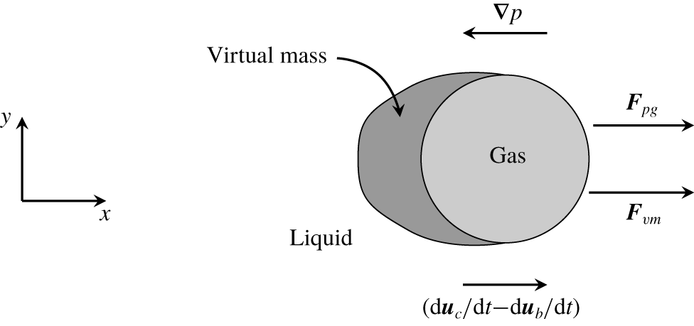
Figure 3. Forces acting on a bubble owing to pressure gradient and virtual mass.
Rapid growth and collapse processes of a bubble introduce a force that depends on the rate of change of the bubble’s volume. According to Johnson & Hsieh (Reference Johnson and Hsieh1966) this force is written as follows:
 $$\begin{eqnarray}\boldsymbol{F}_{volume}=\frac{\unicode[STIX]{x1D70C}_{c}}{2}\frac{\text{d}V_{b}}{\text{d}t}(\boldsymbol{u}_{c}-\boldsymbol{u}_{b})=\frac{3}{2}\unicode[STIX]{x1D70C}_{c}V_{b}\frac{{\dot{R}}}{R}(\boldsymbol{u}_{c}-\boldsymbol{u}_{b}),\end{eqnarray}$$
 where  ${\dot{R}}$ is the radius growth rate or velocity of the bubble wall. The radius growth rate as well as the relative velocity between carrier fluid and bubble determine the direction of this force. The relative velocity causes also a drag force exerted on the bubble, which is written as follows:
 $$\begin{eqnarray}\boldsymbol{F}_{drag}=\frac{3}{4}c_{D}m_{eff}\unicode[STIX]{x1D707}_{c}\frac{1}{\unicode[STIX]{x1D70C}_{b}(2.0R)^{2}}|\boldsymbol{u}_{c}-\boldsymbol{u}_{b}|(\boldsymbol{u}_{c}-\boldsymbol{u}_{b}).\end{eqnarray}$$
 The effective mass of the bubble,  $m_{eff}=m_{b}+m_{a}$, consists of the bubble mass, $m_{b}=\unicode[STIX]{x1D70C}_{b}V_{b}$, and the added mass, $m_{a}=\frac{1}{2}\unicode[STIX]{x1D70C}_{c}V_{b}$. The drag coefficient according to Haberman & Morton (Reference Haberman and Morton1953) reads as follows:
 $$\begin{eqnarray}c_{D}=24.0(1.0+0.197Re_{b}^{0.63}+2.6\cdot 10^{-4}Re_{b}^{1.38}),\end{eqnarray}$$
 where  $Re_{b}=(\unicode[STIX]{x1D70C}_{c}|\boldsymbol{u}_{c}-\boldsymbol{u}_{b}|2R)/\unicode[STIX]{x1D707}_{c}$ is the bubble Reynolds number. In fluids where the effects of gravity exceed the effects from the flow, the drag force is alternatively defined as follows (Darmana, Deen & Kuipers Reference Darmana, Deen and Kuipers2006):
 $$\begin{eqnarray}\boldsymbol{F}_{drag,grav}={\textstyle \frac{1}{2}}c_{D,E\ddot{o} }\unicode[STIX]{x1D70C}_{c}\unicode[STIX]{x03C0}R^{2}|\boldsymbol{u}_{c}-\boldsymbol{u}_{b}|(\boldsymbol{u}_{c}-\boldsymbol{u}_{b}).\end{eqnarray}$$
 In this case, the drag coefficient is  $c_{D,E\ddot{o} }=\frac{8}{3}E\ddot{o} /(E\ddot{o} +4)$ with the Eötvös number $E\ddot{o} =(\unicode[STIX]{x1D70C}_{c}-\unicode[STIX]{x1D70C}_{b})\boldsymbol{g}(2R)^{2}/\unicode[STIX]{x1D70E}$, and $\boldsymbol{g}=(0,0,-9.81)~\text{m}~\text{s}^{-2}$ is the vector of gravitational acceleration.
According to Saffman (Reference Saffman1965) bubbles are subject to lift forces caused by the surrounding shear flows. This lift force is defined as follows:
 $$\begin{eqnarray}\boldsymbol{F}_{lift}={\textstyle \frac{3}{8}}c_{L}\unicode[STIX]{x1D70C}_{c}V_{b}\frac{(\boldsymbol{u}_{c}-\boldsymbol{u}_{b})}{\unicode[STIX]{x1D6FC}_{S}}\times \unicode[STIX]{x1D74E},\end{eqnarray}$$
 with the lift coefficient,  $c_{L}$, and the dimensionless shear rate
 $$\begin{eqnarray}\unicode[STIX]{x1D6FC}_{S}=\frac{|\unicode[STIX]{x1D74E}|R}{|\boldsymbol{u}_{c}-\boldsymbol{u}_{b}|},\end{eqnarray}$$
 where  $\unicode[STIX]{x1D74E}=\unicode[STIX]{x1D735}\times \boldsymbol{u}_{c}$ is the vorticity of the flow. The lift coefficient, $c_{L}$, depends on the bubble’s Reynolds number and the dimensionless shear rate.
Owing to the density difference between carrier fluid and the vapour-filled bubble, a buoyancy force
 $$\begin{eqnarray}\boldsymbol{F}_{gravity}=(\unicode[STIX]{x1D70C}_{b}-\unicode[STIX]{x1D70C}_{c})\boldsymbol{g}V_{b}\end{eqnarray}$$
acts on the bubble, which lets bubbles rise in liquids of higher density.
Figure 4 depicts the forces owing to Saffman lift, gravity, drag and volume variation, which influence the bubble’s momentum. With  $u_{c,x}$ as the $x$-component of velocity, $\boldsymbol{u}$, the lift force results from the positive velocity gradient in the $y$-direction, $\unicode[STIX]{x2202}u_{c,x}/\unicode[STIX]{x2202}y$. The high flow velocity along the bubble’s top wall generates a low pressure region, and the lower flow velocity along the bubble’s bottom wall generates a high pressure region. This pressure difference causes a lift force, $\boldsymbol{F}_{lift}$, pointing in the positive $y$-direction. The gravitational acceleration acts in the negative $y$-direction, generating a rising force, $\boldsymbol{F}_{gravity}$, on the bubble that is attributed to the lower gas density inside the bubble compared to the density of the surrounding liquid. The drag force, $\boldsymbol{F}_{drag}$, acts in the positive $x$-direction because the bubble’s velocity, $\boldsymbol{u}_{b}$, and the carrier fluid velocity, $\boldsymbol{u}_{c}$, act in this direction (and $\boldsymbol{u}_{b}<\boldsymbol{u}_{c}$). The relative velocity between carrier fluid and bubble, $(\boldsymbol{u}_{c}-\boldsymbol{u}_{b})$, and the bubble growth rate, ${\dot{R}}$, point in the positive $x$-direction and, therefore, cause a volume variation force, $\boldsymbol{F}_{volume}$, that is also positive.
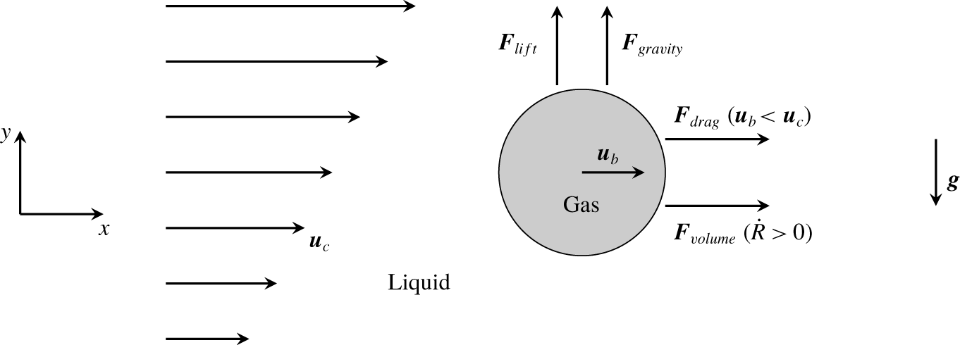
Figure 4. Forces acting on a bubble owing to Saffman lift, gravity, drag and volume variation.
The virtual mass force (3.25) comprises two parts. One part is proportional to the bubble’s acceleration,  $\text{d}\boldsymbol{u}_{b}/\text{d}t$; the other part, to the acceleration of the surrounding liquid, $\text{d}\boldsymbol{u}_{c}/\text{d}t$. Moving the part proportional to bubble acceleration to the left-hand side and the term proportional to the fluid acceleration to the right-hand side of (3.23) yields the following expression:
 $$\begin{eqnarray}m_{eff}\frac{\text{d}\boldsymbol{u}_{b}}{\text{d}t}=\mathop{\sum }_{i}\boldsymbol{F}_{i}.\end{eqnarray}$$
 Thus, the part of the virtual mass force proportional to  $\text{d}\boldsymbol{u}_{c}/\text{d}t$ and the pressure force are considered together, and time integration via a semi-implicit approach then gives velocities
 $$\begin{eqnarray}\boldsymbol{u}_{b}^{n+1}+\frac{\unicode[STIX]{x0394}t}{m_{eff}}\boldsymbol{F}^{n+1}=\boldsymbol{u}_{b}^{n}+\frac{\unicode[STIX]{x0394}t}{m_{eff}}\boldsymbol{F}^{n},\end{eqnarray}$$
 where  $\boldsymbol{u}_{b}^{n+1}$ is the bubble velocity of the next time step, $\boldsymbol{u}_{b}^{n}$ the bubble velocity of the last time step and $\unicode[STIX]{x0394}t$ the time step. The implicitly treated forces, denoted as $\boldsymbol{F}^{n+1}$, represent parts of the drag and volume variation forces proportional to the bubble velocity. Parts of the drag and volume variation forces proportional to the carrier fluid velocity are naturally included in the explicit forces, denoted as $\boldsymbol{F}^{n}$. All other forces are treated explicitly. Integrating the bubble velocity over time then yields the bubble position, $\boldsymbol{x}_{b}$:
 $$\begin{eqnarray}\frac{\text{d}\boldsymbol{x}_{b}}{\text{d}t}=\boldsymbol{u}_{b}.\end{eqnarray}$$
3.3 Single bubble dynamics
Computations based on different forms of the Rayleigh–Plesset equation (Rayleigh Reference Rayleigh1917; Plesset Reference Plesset1949) give the dynamics of spherical bubbles. Following the formulation of Brennen (Reference Brennen2005) and including the effect of relative velocity (Hsiao et al. Reference Hsiao, Chahine and Liu2000) the Rayleigh–Plesset equation is written as follows:
 $$\begin{eqnarray}\frac{p_{b}-p}{\unicode[STIX]{x1D70C}_{l}}=R\ddot{R}+\frac{3}{2}{\dot{R}}^{2}+\frac{4\unicode[STIX]{x1D708}_{l}{\dot{R}}}{R}+\frac{2\unicode[STIX]{x1D70E}}{\unicode[STIX]{x1D70C}_{l}R}-\frac{(\boldsymbol{u}-\boldsymbol{u}_{b})^{2}}{4},\end{eqnarray}$$
 where  $R$,
$R$,  ${\dot{R}}$, $\ddot{R}$ are the bubble radius, bubble wall velocity and bubble wall acceleration, respectively; $p$ is the pressure in the carrier fluid at the bubble position, $\unicode[STIX]{x1D70E}$ is the surface tension of water and $\unicode[STIX]{x1D708}_{c}$ is the kinematic viscosity of the carrier fluid; $p_{b}=p_{v}+p_{g}$ is the pressure in the bubble with the pressure of non-condensable gas in the bubble, $p_{g}$. The gas changes its state isentropically according to the relation $p_{g}=p_{g0}(R_{0}/R)^{3\unicode[STIX]{x1D6FE}}$, where $p_{g0}$ and $R_{0}$ are the initial gas pressure and the initial nuclei radius, respectively. The isentropic exponent of $\unicode[STIX]{x1D6FE}=\frac{4}{3}$ represents an adiabatic process. Depending on the flow problem considered, for bubbles with volumes greater than the volumes of the cells they are located in, the pressure in the carrier fluid, $p$, and the velocity in the carrier fluid $\boldsymbol{u}$, are averaged based on the values of control volumes at multiple coordinates at the outer bubble wall (Hsiao et al. Reference Hsiao, Chahine and Liu2000). This approach prevents a bubble growing unrealistically large when its centre is located inside a low pressure region although its surface is already located in a higher pressure region. This enables a more realistic description of bubble behaviour (Hsiao et al. Reference Hsiao, Chahine and Liu2003). For bubbles, with volumes smaller than the volume of the cell they are located in, the last term on the right-hand side of (3.36), proportional to the relative velocity between bubble and carrier fluid, is neglected because it is multiple orders of magnitude smaller than the other terms (e.g. terms proportional to surface tension or $(p_{b}-p)$).
According to Tomita & Shima (Reference Tomita and Shima1977), during bubble collapse, the bubble wall attains velocities in the range of the speed of sound of the liquid. The effect of liquid compressibility must be considered because shock waves form after the collapse affecting the behaviour of subsequent bubble rebounds. Based on this equation for a spherical bubble in a viscous compressible liquid, Mathew, Keith & Nikolaidis (Reference Mathew, Keith and Nikolaidis2006) formulated the following expression for bubble dynamics:
 $$\begin{eqnarray}\frac{p_{r=R}-p}{\unicode[STIX]{x1D716}\unicode[STIX]{x1D70C}_{c}}+\frac{R{\dot{p}}_{r=R}}{\unicode[STIX]{x1D716}\unicode[STIX]{x1D70C}_{c}c_{\infty }}=R\ddot{R}\left[1-(1+\unicode[STIX]{x1D716})\frac{{\dot{R}}}{c_{\infty }}\right]+\frac{3}{2}{\dot{R}}^{2}\left(\frac{4-\unicode[STIX]{x1D716}}{3}-\frac{4}{3}\frac{{\dot{R}}}{c_{\infty }}\right),\end{eqnarray}$$
with
 $$\begin{eqnarray}\unicode[STIX]{x1D716}=1-\frac{\unicode[STIX]{x1D70C}_{b}}{\unicode[STIX]{x1D70C}_{c}}=0.99881.\end{eqnarray}$$
 Applying the first-order correction to the pressure  $p_{r=R}$ at the bubble wall leads to the following relation (Tomita & Shima Reference Tomita and Shima1977):
 $$\begin{eqnarray}p_{r=R}=p_{g,0}\left(\frac{R_{0}}{R}\right)^{3\unicode[STIX]{x1D6FE}}-\frac{2\unicode[STIX]{x1D70E}}{R}-\unicode[STIX]{x1D716}4\unicode[STIX]{x1D707}_{c}\frac{{\dot{R}}}{R},\end{eqnarray}$$
and its derivative
 $$\begin{eqnarray}{\dot{p}}_{r=R}=-3\unicode[STIX]{x1D6FE}p_{g,0}\frac{{\dot{R}}}{R}\left(\frac{R_{0}}{R}\right)^{3\unicode[STIX]{x1D6FE}}+\frac{2\unicode[STIX]{x1D70E}}{R^{2}}{\dot{R}}-\unicode[STIX]{x1D716}4\unicode[STIX]{x1D707}_{c}\frac{\ddot{R}R-{\dot{R}}^{2}}{R^{2}}.\end{eqnarray}$$
 Depending on the sign of the bubble wall velocity from the previous time step, equation (3.36) (growth) or equation (3.37) (collapse) is solved to obtain  $\ddot{R}$ for each bubble individually. Although the difference in computational cost is negligible for most hybrid simulations, whether equation (3.36) or equation (3.37) is solved, it becomes more remarkable for larger numbers of bubbles. Then, ${\dot{R}}$ and $R$ are calculated using the trapezoidal rule for the implicit second-order time integration. Adaptive time stepping enables the efficient calculation of $\ddot{R}$ over the relatively long growth phase and the shorter collapse phase. The bubble dynamics equation is time integrated over the entire time step of the Eulerian flow solution.
3.4 Interaction between Eulerian and Lagrangian frame
The continuous liquid phase and the cavitation bubbles interact with each other in different ways. Effects of the continuous phase on the vapour phase are already considered in forces influencing transport and dynamics of a bubble. For a one-way coupled simulation, only influences of the liquid phase on the vapour bubbles are considered but not vice versa. As soon as the bubbles affect also the carrier phase, we speak of a two-way coupling. As mostly isolated Lagrangian bubbles are introduced during vapour transformations from the Eulerian into the Lagrangian frame, collision and coalescence of Lagrangian bubbles with each other were neglected. Break-up processes of Lagrangian bubbles into multiple smaller bubbles, which would mostly occur after the first collapse phase, were neglected because their contribution to damage is supposedly negligible. Analogously to the Euler–Euler cavitation models, the properties of the homogeneous mixture are calculated using volume fractions for the liquid and vapour phases. The volume fraction for vapour structures in the Eulerian frame,  $\unicode[STIX]{x1D6FC}_{v,E}$, is calculated from the vapour volume fraction equation (3.12). In contrast to an Eulerian treatment of the vapour phase, a Lagrangian treatment does not require the solution of a transport equation for the volume fraction. Transport and dynamics of the vapour phase are obtained from the behaviour of the single bubbles. Thus, to obtain a volume fraction of vapour, the vapour volume fraction in control volumes occupied by Lagrangian bubbles, $\unicode[STIX]{x1D6FC}_{v,L}$, is calculated by distributing the entire vapour volume of the Lagrangian bubbles to the surrounding control volumes of the Eulerian grid. Using a one-way coupling technique would violate mass conservation because the vapour volume would be excluded from the Eulerian frame when substituting a Lagrangian bubble. Moreover, for a one-way coupling, pressure and velocity distributions in the carrier fluid surrounding the bubbles would be incorrect. Using a two-way coupling approach, made it possible to always fully transform vapour volumes between frames. Thus, mass and momentum were fully conserved. As the trajectories of Lagrangian particles may deviate from the streamlines of the carrier fluid flow, an additional source term was added to account for the influence of Lagrangian bubbles on the momentum of the carrier fluid. For two-way coupled Euler–Lagrange methods, a distribution becomes problematic when a high density of bubbles per liquid causes bubbles to overlap. A four-way coupling that accounts for bubble–bubble interactions (collisions and coalescence) can then be used. However, in our hybrid approach, overlapping of bubbles is unlikely to occur, because agglomerations of bubbles are treated in the Eulerian frame. Therefore, Lagrangian bubbles were two-way coupled with the liquid phase.
The total vapour volume fraction in the domain is obtained by adding the vapour volume fractions from the Eulerian and the Lagrangian frameworks
 $$\begin{eqnarray}\unicode[STIX]{x1D6FC}_{v,total}=\unicode[STIX]{x1D6FC}_{v,E}+\unicode[STIX]{x1D6FC}_{v,L}.\end{eqnarray}$$
Then, the density and viscosity of the mixture fluid are updated according to (3.1).
In the pressure equation (3.11), the total vapour volume fraction,  $\unicode[STIX]{x1D6FC}_{v,total}$, is used to calculate the source terms (3.18). The implicit treatment of the pressure in (3.11) yields a stable system of equations. Although it is possible to calculate the source terms on the right hand side of (3.9) based on bubble properties ( $R$,
$R$,  ${\dot{R}}$), such approaches cause instabilities because, in contrast to the approach of Sauer (Reference Sauer2000), the source terms cannot be treated implicitly.
Furthermore, the source term,  $\boldsymbol{s}_{b}$, in the momentum equation (3.3), considers the influence of Lagrangian bubbles on the momentum of the carrier fluid. The source term depends on the rate of change of the bubble velocity of all bubbles entering a considered control volume. When a Lagrangian bubble enters a control volume, a new time step to calculate the bubble velocity is started. Solving (3.33) yields the rate of change of the bubble velocity. The source term in the momentum equation for a given cell $j$ is then defined as follows (Vallier Reference Vallier2013; Lidtke Reference Lidtke2017):
 $$\begin{eqnarray}\boldsymbol{s}_{b,j}=-\frac{1}{V_{j}}\mathop{\sum }_{i}m_{eff,i}\frac{\boldsymbol{u}_{b,i}^{n+1}-\boldsymbol{u}_{b,i}^{n}}{\unicode[STIX]{x0394}t},\end{eqnarray}$$
 accounting for the contribution from all bubbles of index  $i$ incorporated in the cell; $n$ denotes the considered Eulerian time step.
3.5 Hybrid multi-scale treatment of vapour phase
There are several advantages associated with Euler–Euler and Euler–Lagrange methods to simulate cavitation. An Eulerian treatment of the vapour phase enables fast simulations while neglecting single bubble behaviour. A Lagrangian treatment of the vapour phase consisting of spherical bubbles yields more accurate simulations of bubble behaviour; however, the computational effort is high. Furthermore, a Lagrangian approach requires knowing the size and distribution of nuclei in the water, particulars that are usually not known. Regarding erosion assessment, it seems advantageous to combine both approaches and to use a Lagrangian approach only when the Eulerian approach cannot resolve the vapour structures. Therefore, we used a hybrid approach based on earlier techniques of Vallier (Reference Vallier2013), Lidtke (Reference Lidtke2017) and Ma et al. (Reference Ma, Hsiao and Chahine2017). The macroscopic vapour volumes are dealt with in the Eulerian frame; the motion and dynamics of microscopic cavitation bubbles, in the Lagrangian frame.
Cavitation structures are then transformed from the Eulerian into the Lagrangian frame and vice versa. Vapour volumes underresolved by the Eulerian frame are transformed into spherical Lagrangian bubbles. Isolated vapour volumes are identified by selecting all control volumes containing a minimum threshold of vapour volume fraction  $\unicode[STIX]{x1D6FC}_{v,limit}$. Afterwards, the isolated vapour volumes are evaluated based on their size relative to the numerical grid and their absolute size. Transformation into the Lagrangian frame is performed if the vapour structure contains less than a threshold number of control volumes, $n_{limit}$, or if the radius representing the volume of the vapour structure is smaller than a threshold radius, $R_{limit}$. Analogously, transformation of Lagrangian vapour bubbles into the Eulerian frame takes place, when the above threshold values are exceeded again. Additionally, Lagrangian bubbles in contact with larger vapour structures in the Eulerian frame are merged into these larger vapour volumes and transformed into the Eulerian frame.
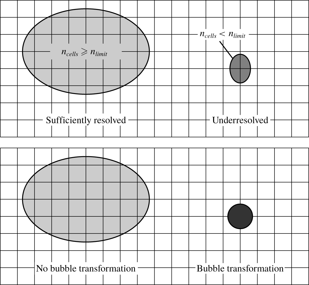
Figure 5. Evaluation of vapour structures in the Eulerian frame; underresolved vapour volumes are replaced by spherical Lagrangian bubbles.
Vapour structures can be transformed in both directions between the Eulerian and the Lagrangian frame. A vapour structure in the Eulerian frame can be defined as underresolved when its representative radius falls below a threshold radius,  $R_{limit}$, or when the vapour volume on the Eulerian grid contains less than a threshold number of vapour filled cells, $n_{limit}$. Figure 5 shows an example of the evaluation of two vapour structures. The left vapour structure is sufficiently resolved on the Eulerian grid ( $n_{cells}\geqslant n_{limit}$), whereas the right vapour structure is underresolved ( $n_{cells}<n_{limit}$). Therefore, the right vapour structure is transformed into the Lagrangian frame and replaced by a spherical Lagrangian bubble of equivalent vapour volume.
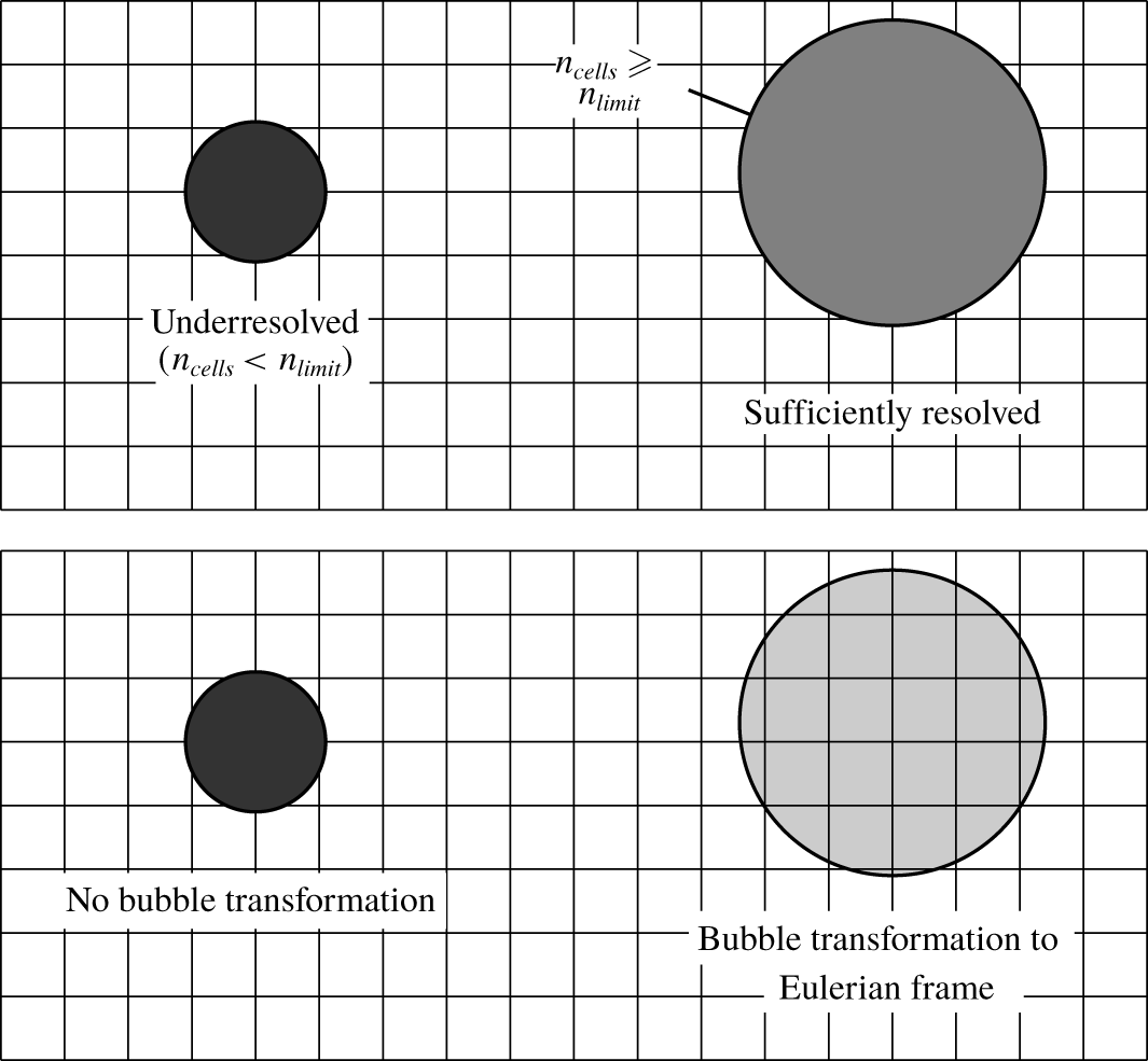
Figure 6. Evaluation of Lagrangian bubbles; bubbles are transformed when they can be sufficiently resolved by the numerical mesh.
Similarly, Lagrangian bubbles are transformed into vapour volumes on the Eulerian grid. When Lagrangian bubbles grow and exceed the limiting number of cells,  $n_{limit}$, they are transformed into the Eulerian frame because then the vapour volume can be sufficiently resolved by the numerical mesh. Figure 6 shows the evaluation of Lagrangian bubbles. The left bubble is too small to be transformed into the Eulerian frame because it overlaps too few cells. However, the bubble on the right overlaps enough cells to be transformed into the Eulerian frame because it can be sufficiently resolved.
Another mechanism to transform a Lagrangian vapour volume into an Eulerian one takes place when a Lagrangian bubble touches a vapour structure in the Eulerian frame. Figure 7 depicts the scenario of a Lagrangian bubble touching a vapour cloud in the Eulerian frame. Although the isolated bubble is too small to be sufficiently resolved by the numerical grid, it is identified as touching the vapour cloud and, therefore, transformed into the Eulerian frame, i.e. the bubble merges into the larger vapour structure.
To prevent bubbles from being transformed back and forth between frames, Lagrangian bubbles just transformed, cannot be retransformed into the Eulerian frame within the same time step. This ensures that the bubble dynamics is continuously developed for a longer time.
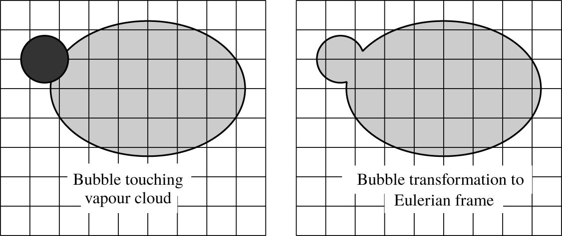
Figure 7. Lagrangian bubble transformed into the Eulerian frame as it touches a vapour cloud.
Special treatment is required for parallel simulations involving the above transformation processes. If transformations are just treated locally, vapour structures overlapping processor boundaries by a small amount may cause transformations from the Eulerian into the Lagrangian frame because the vapour volume on the local processor is small. Thus, sizes of vapour structures need to be communicated between processors to determine the global volume of a vapour structure in the domain. For full parallelisation, we implemented an algorithm similar to the one of Lidtke (Reference Lidtke2017), allowing us to evaluate properties of the global instead of the local vapour volumes.
3.6 Non-condensable gas content of Lagrangian bubbles
When an Eulerian vapour volume is transformed into a spherical bubble in the Lagrangian framework, not only the vapour volume, but also the non-condensable gas content inside the bubble needs to be considered. Depending on the mass of this non-condensable gas, the bubble’s equilibrium radius is defined and, consequently, oscillations involving growth and collapse are significantly influenced. In most cavitating flows, the size distribution of cavitation nuclei in forms of gas bubbles is unknown. Therefore, constant nuclei sizes are often assumed for numerical simulations involving Lagrangian methods. More complex approaches adopt a Gauss or Rayleigh distribution of the nuclei in a flow.
A more realistic distribution of nuclei was derived from optical measurements. Reuter et al. (Reference Reuter, Lesnik, Ayaz-Bustami, Brenner and Mettin2018) conducted bubble size measurements in various structures of acoustically generated cavitation. They investigated a hydrodynamic jet where no cavitation appeared at the beginning. Therefore, it resembled a standard hydrodynamic case. The acoustic sound field then caused the cavitation nuclei to grow to larger cavitation bubbles, making them visible and making it possible to capture their dynamics. Based on high-speed observations of bubble sizes and using an equation for spherical bubble dynamics, they determined populations of equilibrium sizes of bubbles. For different cavitation structures, they measured the distribution of nuclei and obtained the distribution of equilibrium radii for  $R_{0}>2.2~\unicode[STIX]{x03BC}\text{m}$. They found that the sum of an exponential decay and a Gaussian distribution resulted in the best fit expressed as follows:
 $$\begin{eqnarray}F_{1}=\exp \left(-\frac{R_{0}}{x_{1}}\right)+x_{3}\frac{1}{\sqrt{2\unicode[STIX]{x03C0}{x_{2}}^{2}}}\exp \left(-\frac{{R_{0}}^{2}}{2{x_{2}}^{2}}\right),\end{eqnarray}$$
 with  $x_{1}=1.28~\unicode[STIX]{x03BC}\text{m}$, $x_{2}=0.54~\unicode[STIX]{x03BC}\text{m}$ and $x_{3}=0.0838$ for the case of a cavitating jet. Smaller equilibrium radii of $R_{0}<2.2~\unicode[STIX]{x03BC}\text{m}$ could not be measured because the optical resolution was limited. Smaller bubbles did not oscillate to sizes large enough to be measured because of the high surface tension of bubbles below the threshold by Blake, Mettin et al. (Reference Mettin, Akhatov, Parlitz, Ohl and Lauterborn1997). To obtain a measurement-based nuclei distribution, we normalised the distribution of Reuter et al. (Reference Reuter, Lesnik, Ayaz-Bustami, Brenner and Mettin2018) and combined it with a simple quadratic polynomial as follows:
 $$\begin{eqnarray}F(R_{0})=\left\{\begin{array}{@{}l@{}}\displaystyle F_{1}=\left(\exp \left(-\frac{R_{0}}{x_{1}}\right)+x_{3}\frac{1}{\sqrt{2\unicode[STIX]{x03C0}{x_{2}}^{2}}}\exp \left(-\frac{{R_{0}}^{2}}{2{x_{2}}^{2}}\right)\right)/x_{4}\quad \text{if }R_{0}>2.2~\unicode[STIX]{x03BC}\text{m}\quad \\ F_{2}=(a_{1}{R_{0}}^{2}+a_{2}R_{0})/a_{3}\quad \text{else},\quad \end{array}\right.\end{eqnarray}$$
 with the constants  $x_{4}=1.328005544$, $a_{1}=-0.00883577$, $a_{2}=0.03711025$, $a_{3}=0.2879407$ and the aforementioned values of $x_{1}$, $x_{2}$ and $x_{3}$ for the cavitating jet. Figure 8 displays the combined distribution.
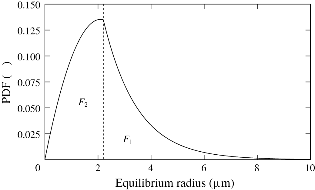
Figure 8. Probability density function (PDF) of different bubble equilibrium radii.
3.7 Erosion assessment
3.7.1 Eulerian approach
We employed a numerical model to estimate cavitation erosion for our Euler–Euler simulations. Based on the approach of Peters et al. (Reference Peters, Lantermann and el Moctar2015a,Reference Peters, Sagar, Lantermann and el Moctarb) this model determines the presence of vapour in the near-wall region at every numerical face of a considered boundary and in the numerical domain within its vicinity – referred to as a cell zone. This is done by evaluating the volume fraction of vapour,  $\unicode[STIX]{x1D6FC}_{v}$, if it exceeds a certain threshold value, $\unicode[STIX]{x1D6FC}_{limit,ero}$. Earlier investigations found that a threshold value of $\unicode[STIX]{x1D6FC}_{limit,ero}=0.01$ is reasonable to determine whether enough vapour is inside a control volume to be considered.
The erosion model relies on the hypothesis that a liquid high velocity water jet, a so-called microjet, is developed when a cavitation bubble collapses near a solid surface. The magnitude of the microjet velocity depends on the distance of the bubble from this surface, the size of the bubble and the pressure of the liquid surrounding the bubble. As soon as the microjet velocity exceeds a certain threshold velocity, referred to as the critical velocity, an erosion impact is supposed to occur. Models to approximate the impact pressure caused by a microjet on a solid surface rely on the water hammer relationship of Joukowsky (Reference Joukowsky1898). Knapp, Daily & Hammitt (Reference Knapp, Daily and Hammitt1970) formulated the pressure rise induced by a collapsing bubble as follows:
 $$\begin{eqnarray}p^{\prime }=\unicode[STIX]{x1D70C}c\unicode[STIX]{x0394}v,\end{eqnarray}$$
 where  $\unicode[STIX]{x1D70C}$ is the density of the liquid, $c$ is the acoustic velocity at the bubble wall, $v$ is the velocity of the bubble wall and $\unicode[STIX]{x0394}v$ is the velocity at the beginning and end of the bubble collapse. Dular et al. (Reference Dular, Stoffel and Širok2006) and Dular & Coutier-Delgosha (Reference Dular and Coutier-Delgosha2009) used this hypothesis to numerically assess cavitation erosion. Peters et al. (Reference Peters, Lantermann and el Moctar2015a,Reference Peters, Sagar, Lantermann and el Moctarb) extended this numerical erosion model, taking into account flow quantities in the neighbouring volume surrounding the regarded surface. These numerical models provide reliable qualitative estimates of cavitation erosion on various surfaces. The microjet velocity is therein calculated as follows:
 $$\begin{eqnarray}v_{jet}=c_{\unicode[STIX]{x1D6FE}}\sqrt{\frac{p-p_{v}}{\unicode[STIX]{x1D70C}_{l}}}.\end{eqnarray}$$
It is assumed that an impact that damages a surface occurs when the critical velocity is exceeded. This critical velocity is defined as follows (Lush Reference Lush1983):
 $$\begin{eqnarray}v_{crit}=\sqrt{\frac{\unicode[STIX]{x1D70E}_{y}}{\unicode[STIX]{x1D70C}_{l}}\left(1-\left(1+\frac{\unicode[STIX]{x1D70E}_{y}}{B}\right)^{-1/n}\right)},\end{eqnarray}$$
 which relates the yield strength,  $\unicode[STIX]{x1D70E}_{y}$, to the critical velocity, needed to cause plastic flow of the impacted material. The Tait equation of state accounts for the compressibility of the liquid mass impacting the solid surface. $B=300~\text{MPa}$ and $n=7$ are standard coefficients of liquid water in the Tait equation. The dimensionless impact intensity, $c_{jet}$, equals the ratio of the microjet velocity and the critical velocity as follows:
 $$\begin{eqnarray}c_{jet}=\frac{v_{jet}}{v_{crit}}.\end{eqnarray}$$
Based on the approach of Peters et al. (Reference Peters, Lantermann and el Moctar2015a,Reference Peters, Sagar, Lantermann and el Moctarb) dimensionless erosion potential equals the ratio of estimated erosion at every face of a surface and the total estimated erosion on the surface. The cumulative erosion potential for an Eulerian assessment is then calculated as follows:
 $$\begin{eqnarray}c_{ero,E}=\frac{\displaystyle \mathop{\sum }_{t}^{T}c_{jet,t}}{\displaystyle \mathop{\sum }_{n}^{N}\mathop{\left(\mathop{\sum }_{t}^{T}c_{jet,t}\right)}\nolimits_{n}},\end{eqnarray}$$
 where  $t$ is the time, $T$ is the time interval of erosion assessment, $n$ is the face number and $N$ is the total number of eroded faces. Larger values of this potential indicate a higher erosion potential, and a value of zero denotes that no erosion occurs. Erosion is estimated at the end of every time step of the flow solution.
Although this erosion model relies on the microjet hypothesis, it can be substituted by other hypotheses, such as one that is based on a simplified calculation of the collapse pressure during a bubble collapse. We found that both Eulerian models obtained similar results. In former investigations, we used the microjet model to assess erosion for an axisymmetric nozzle and for a propeller and obtained favourable agreements with measurements (Peters et al. Reference Peters, Lantermann and el Moctar2015a,Reference Peters, Sagar, Lantermann and el Moctarb, Reference Peters, Lantermann and el Moctar2018).
3.7.2 Lagrangian approach
Resolving shock wave radiation for asymmetric bubble collapses in a macroscopic flow simulation is almost impossible, because the computational effort would be excessive. To directly numerically simulate the multi-scale flow dynamics and the associated structural interaction may still be unrealistic. Therefore, we chose to assess erosion based on spherical Lagrangian bubble collapses and mathematically modelled the physics involved in an asymmetric near-wall bubble collapse based on well-recognised fundamental experiments and theoretical considerations that are not restricted to particular applications. Our erosion model accounts for various phenomena during an asymmetric bubble collapse, such as (i) the motion of the bubble’s centre towards the solid surface, (ii) the reduced collapse pressure attributed to the non-spherical collapse and (iii) the pressure decay of the shock wave that travels towards the solid surface.
After the collapse of a bubble, a shock occurs. Shock waves of large pressure amplitudes are radiated spherically away from the bubble. Depending on the damping of the radiated pressures, shock waves are able to damage a nearby surface. Acoustic waves travel at velocities equal to the sound velocity of the medium they permeate. After collapse, the pressure is assumed to decay linearly as the acoustic wave expands. We define the following ratio:
 $$\begin{eqnarray}\frac{p_{1}}{p_{0}}=\frac{r_{0}}{r_{1}}.\end{eqnarray}$$
 Here, the indices  $0$ and $1$ denote the start and end position of a spherically expanding acoustic wave, respectively, $r_{i}$ is the radius of the acoustic wave and $p_{i}$ is the pressure at the wave’s considered radius. The sound velocity of liquid water is about $c=1450~\text{m}~\text{s}^{-1}$. Although, after generation, shock waves usually travel at velocities greater than the sound velocity. In this case, a nonlinear relation applies, written as follows:
 $$\begin{eqnarray}\frac{p_{1}}{p_{0}}=\left(\frac{r_{0}}{r_{1}}\right)^{n_{shock}}.\end{eqnarray}$$
 Vogel, Busch & Parlitz (Reference Vogel, Busch and Parlitz1996) studied laser-induced bubbles. They found the pressure after collapse to decay with  $n_{shock}\approx 2.0$ for pressures over 100 MPa and with $n_{shock}\approx 1.06$ for lower pressures. Noack & Vogel (Reference Noack and Vogel1998) and Lauterborn & Vogel (Reference Lauterborn and Vogel2013) investigated shock waves generated at collapses of laser-induced bubbles. Although they found initial shock velocities of up to $5000~\text{m}~\text{s}^{-1}$ and pressures up to 11 GPa, the shock waves were rapidly damped. Noack & Vogel (Reference Noack and Vogel1998) found that the damping of the shock pressure up to a distance of $r_{1}\leqslant 2r_{0}$ was about $n_{shock}=1.3\pm 0.2$. For shock wave expansions of $r_{1}>2r_{0}$, the pressures were decreasing at a rate of $n_{shock}=2.2\pm 0.1$. Supponen et al. (Reference Supponen, Obreschkow, Kobel, Tinguely, Dorsaz and Farhat2017) stated a pressure decay for laser-induced bubbles proportional to $n_{shock}=1.249\pm 0.003$ obtained from a fitted function. Johnsen & Colonius (Reference Johnsen and Colonius2008) numerically investigated shock-induced collapses of gas bubbles and found that the pressure decay of shocks is proportional to $n_{shock}=1.0$.
During the collapse of a bubble, liquid water flows towards the bubble from all sides. In the vicinity of a rigid boundary, a bubble always collapses asymmetrically because the flow towards the bubble is disturbed by the presence of the solid wall. Therein, a high liquid microjet pierces the bubble and impacts on the rigid surface. Simultaneously, the flow of the microjet produces a toroidal bubble that collapses immediately after impact of the microjet. During the entire collapse process, the bubble moves towards the solid surface, and its impact concentrates in direction of the surface. The following dimensionless stand-off distance,  $\unicode[STIX]{x1D6FE}$, is often used to classify single bubble collapses in the vicinity of rigid boundaries
 $$\begin{eqnarray}\unicode[STIX]{x1D6FE}=\frac{H}{R_{max}}.\end{eqnarray}$$
 Here,  $H$ is the distance of the bubble centre from the rigid boundary and $R_{max}$ is the maximum bubble radius at the beginning of collapse. Supponen et al. (Reference Supponen, Obreschkow, Tinguely, Kobel, Dorsaz and Farhat2016) considered laser-induced bubbles collapsing in a gravitational field, near a free surface and near a rigid surface. They conducted experiments for different stand-off distances, $\unicode[STIX]{x1D6FE}$, and found that the normalised bubble displacement, $\unicode[STIX]{x0394}z/R_{max}$, is related to a scalar anisotropy parameter, $\unicode[STIX]{x1D701}$, as follows:
 $$\begin{eqnarray}\unicode[STIX]{x0394}z/R_{max}=2.5\unicode[STIX]{x1D701}^{0.6}.\end{eqnarray}$$
 Here,  $\unicode[STIX]{x0394}z$ is the bubble displacement and $\unicode[STIX]{x1D701}\equiv -|\unicode[STIX]{x1D73B}|$ is a scalar anisotropy parameter related to the Kelvin impulse, where $\unicode[STIX]{x1D73B}$ is the vector of the anisotropy parameter. In the case of a bubble near a rigid surface, $\unicode[STIX]{x1D73B}$ is expressed as (Supponen et al. Reference Supponen, Obreschkow, Tinguely, Kobel, Dorsaz and Farhat2016)
 $$\begin{eqnarray}\unicode[STIX]{x1D73B}=-0.195\unicode[STIX]{x1D6FE}^{-2}\boldsymbol{n},\end{eqnarray}$$
 with  $\boldsymbol{n}$ as the unit normal vector of the surface pointing towards the centre of the bubble. Equating (3.53) and (3.54) yields the relation to calculate the motion of a collapsing bubble as a function of its normalised wall distance, $\unicode[STIX]{x1D6FE}$
 $$\begin{eqnarray}\unicode[STIX]{x0394}z=2.5(-|-0.195\unicode[STIX]{x1D6FE}^{-2}\boldsymbol{n}|)^{0.6}R_{max}.\end{eqnarray}$$
 Accordingly, the distance from the bubble centre to the rigid boundary,  $H$, is corrected to obtain $H_{corr}$
 $$\begin{eqnarray}H_{corr}=H+\unicode[STIX]{x0394}z.\end{eqnarray}$$
 Recall that, during collapse,  $\unicode[STIX]{x0394}z$ has a negative sign and a bubble will always move towards the boundary, i.e. $H_{corr}<H$.
Another dependency of the bubble collapse behaviour on  $\unicode[STIX]{x1D6FE}$ is found for the conversion of the bubble energy into energy to generate shock waves. For $\unicode[STIX]{x1D6FE}>4$, Supponen et al. (Reference Supponen, Obreschkow, Kobel, Tinguely, Dorsaz and Farhat2017) conducted experiments of laser-induced bubbles to relate the bubble’s energy to the energy of generated shock waves. For $\unicode[STIX]{x1D6FE}\leqslant 3$, Vogel & Lauterborn (Reference Vogel and Lauterborn1988) experimentally determined that during the first and second collapse of a spherical bubble 60 %–70 % of the energy initially stored in the bubble is converted into shock wave energy. Based on hydrophone measurements, they showed that the emitted shock waves depend on $\unicode[STIX]{x1D6FE}$. For $\unicode[STIX]{x1D6FE}\approx 0.9$, almost no sound is emitted during the first collapse, but more sound is emitted during the second collapse. For $\unicode[STIX]{x1D6FE}$ lower or higher than 0.9 the shock wave emission increases during the first collapse; for $\unicode[STIX]{x1D6FE}$ lower or higher than 1.5, it decreases during the second collapse. Johnsen & Colonius (Reference Johnsen and Colonius2009) numerically investigated non-spherical bubble collapses near solid walls. They found that the fraction of energy that is converted into energy to radiate shock waves during the first bubble collapse increases with increasing distance for $1.0\leqslant \unicode[STIX]{x1D6FE}\leqslant 5.0$. This is in general agreement with the measurements of Vogel & Lauterborn (Reference Vogel and Lauterborn1988).
As the shock wave emission is a result of the collapse pressure of the bubble, we suppose that the pressure generated after a bubble collapse depends on  $\unicode[STIX]{x1D6FE}$ analogously. Based on the experiments of Vogel & Lauterborn (Reference Vogel and Lauterborn1988), we fitted two functions to approximate the radiated pressure for an asymmetric bubble collapse. One function refers to the pressure component after the first collapse, $p_{asym,1}$, and reads as follows:
 $$\begin{eqnarray}\displaystyle p_{asym,1} & = & \displaystyle p_{spher} [\!b_{1}(\unicode[STIX]{x1D6FE}-0.2)^{4}+b_{2}(\unicode[STIX]{x1D6FE}-0.2)^{3}\nonumber\\ \displaystyle & & \displaystyle +\,b_{3}(\unicode[STIX]{x1D6FE}-0.2)^{2}+b_{4}(\unicode[STIX]{x1D6FE}-0.2)+b_{5}\! ],\end{eqnarray}$$
 with  $b_{1}=0.02788$, $b_{2}=-0.35725$, $b_{3}=1.33158$, $b_{4}=-1.38117$ and $b_{5}=0.44444$; $p_{spher}$ is the pressure radiated during the first collapse of a spherically collapsing bubble. The other function refers to the pressure component after the second collapse, $p_{asym,2}$, and reads as follows:
 $$\begin{eqnarray}p_{asym,2}=\left\{\begin{array}{@{}l@{}}p_{spher}(c_{1}\unicode[STIX]{x1D6FE}^{5}+c_{2}\unicode[STIX]{x1D6FE}^{4}+c_{3}\unicode[STIX]{x1D6FE}^{3}+c_{4}\unicode[STIX]{x1D6FE}^{2}+c_{5}\unicode[STIX]{x1D6FE}+c_{6})\quad \text{if }\unicode[STIX]{x1D6FE}\leqslant 2\quad \\ p_{spher}(d_{1}+d_{2}e^{d_{3}\unicode[STIX]{x1D6FE}})\quad \text{else},\quad \end{array}\right.\end{eqnarray}$$
 with the constants  $c_{1}=0.07680$, $c_{2}=-0.46386$, $c_{3}=0.88197$, $c_{4}=-0.60657$, $c_{5}=0.19778$, $c_{6}=0.0006$, $d_{1}=0.03802$, $d_{2}=11.64971$ and $d_{3}=-3.13128$. The sum of these two components gives an approximation for the complete radiated pressure during an asymmetric collapse as follows:
 $$\begin{eqnarray}p_{asym}=p_{asym,1}+p_{asym,2}.\end{eqnarray}$$
 Figure 9 presents our fitted normalised collapse pressure during an asymmetric collapse,  $p_{asym}$, normalised with the collapse pressure emitted during a spherical collapse, $p_{spher}$ and plotted against the normalised stand-off distance, $\unicode[STIX]{x1D6FE}$. Larger collapse pressures are generated for $\unicode[STIX]{x1D6FE}<0.3$ and $\unicode[STIX]{x1D6FE}>1.0$. Recall that for $\unicode[STIX]{x1D6FE}>1.0$, a collapse does not necessarily generate higher pressures at a respective wall because generated shock waves need to travel larger distances over which the pressures decay according to (3.51). Following this approach, we assumed that bubble collapses of about $\unicode[STIX]{x1D6FE}<0.75$ are most aggressive because they take place in contact with a wall and generate high collapse pressures as well.
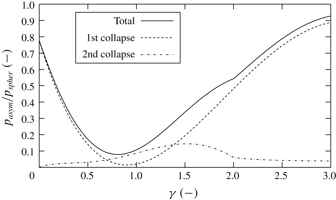
Figure 9. Normalised collapse pressure of an asymmetrical bubble collapse versus normalised stand-off distance fitted to experiments of Vogel & Lauterborn (Reference Vogel and Lauterborn1988).
We conducted simulations with the hybrid Euler–Euler/Euler–Lagrange method to erosion based on information from collapses of spherical Lagrangian bubbles near a solid surface. We first calculated the dynamics of each Lagrangian bubble according to (3.36) and (3.37) and then specified the beginning of the collapse to be the instance when the velocity of the bubble wall,  ${\dot{R}}$, changes sign from negative to positive. Analogously, the beginning of a collapse is found from a change of sign of ${\dot{R}}$ from positive to negative. For all identified collapses, the bubble’s position, its inner bubble pressure, its maximum radius at the beginning of a collapse and its minimum radius after collapse are obtained and serve to assess erosion for a surface.
As only spherical collapses can be calculated using a Lagrangian method, two main effects of the asymmetric collapse behaviour and concentration of a collapse onto a surface are considered. Based on the above discussion, compared to a spherical collapse, during an asymmetric collapse:
(i) the bubble moves towards the rigid surface; and
(ii) the conversion of bubble energy into shock wave energy decreases.
For bubble collapses of  $\unicode[STIX]{x1D6FE}\leqslant 1.0$, we assume that after collapse the bubble is in contact with the rigid wall and the collapse pressure of the bubble is directly exerted on to the surface. For $\unicode[STIX]{x1D6FE}>1$, the Kelvin impulse and (3.55) determine the bubble’s motion towards the rigid surface. Depending on its displacement and radius after collapse, a bubble can be in contact with the surface in which case we calculated the impact pressure on the wall as follows:
 $$\begin{eqnarray}p_{imp}=p_{asym},\end{eqnarray}$$
 where the decreased collapse pressure of a bubble during an asymmetric collapse is determined from (3.57), (3.58) and (3.59). If liquid separates a bubble from the rigid surface, solving (3.51) with  $n_{shock}=2$ gives the bubble’s radiation pressure. This pressure is radiated over a distance until its pressure wave reaches the considered face and causes an impact pressure expressed as follows:
 $$\begin{eqnarray}p_{imp}=p_{asym}\left(\frac{R_{min}}{H_{corr}}\right)^{2}.\end{eqnarray}$$
 Although a microjet impact is not explicitly calculated, the influence of the microjet is incorporated also in the model. First, the motion of the bubble towards the wall is driven by the microjet and accounted for in (3.53) to (3.56). Second, the pressure decay functions from (3.57) to (3.59) take into account the shock wave radiated by the microjet. For different values of  $\unicode[STIX]{x1D6FE}$, the microjet impact on the surface occurs at different times, generates a shock wave and thereby influences the radiation of shock waves.
Analogously to (3.49), the Lagrangian erosion potential,  $c_{ero,L}$, on the considered face is obtained by summing the individual impact pressures, $p_{imp}$, acting on one face and normalised against the sum of all impact pressures on the considered surface
 $$\begin{eqnarray}c_{ero,L}=\frac{\displaystyle \mathop{\sum }_{i}^{I}p_{imp,i}}{\displaystyle \mathop{\sum }_{n}^{N}\mathop{\left(\mathop{\sum }_{i}^{I}p_{imp,i}\right)}\nolimits_{n}},\end{eqnarray}$$
 where index  $i$ refers to the impact itself, and $I$ is the total number of impacts on the regarded face. Similar to (3.49), (3.62) gives the percentage of erosion in one face compared to all faces of the considered surface.
Equation (3.62) assumes a linear relation between erosion and impact pressure,  $p_{imp}$. On the contrary, experiments of Franc & Riondet (Reference Franc and Riondet2006) indicated that incubation times and pit depths depend nonlinearly on impact loads. They also stated that stresses exceeding the yield strength of the material, but not its ultimate strength, are proportional to pit depth, $H_{pit}$, and load stress, $\unicode[STIX]{x1D70E}$. For the material they considered (stainless steel 316 L) and using a Ludwik-type consolidation approach, they proposed the following relationship for the stress range of $\unicode[STIX]{x1D70E}_{y}<\unicode[STIX]{x1D70E}<\unicode[STIX]{x1D70E}_{u}$:
 $$\begin{eqnarray}H_{pit}\propto (\unicode[STIX]{x1D70E}-\unicode[STIX]{x1D70E}_{y})^{2.4}.\end{eqnarray}$$
Although not all our calculated impact pressures are assumed to exceed the yield strength of the regarded material, it is reasonable to assume, similar to (3.63), that our calculated erosion potential is proportional to impact pressure squared. Analogously to equation (3.62), we then calculate the erosion potential as being proportional to the impact pressure squared as follows:
 $$\begin{eqnarray}c_{ero,L2}=\frac{\displaystyle \mathop{\sum }_{i}^{I}{p_{imp,i}}^{2}}{\displaystyle \mathop{\sum }_{n}^{N}\mathop{\left(\mathop{\sum }_{i}^{I}{p_{imp,i}}^{2}\right)}\nolimits_{n}},\end{eqnarray}$$
which also yields the percentage of erosion on one face compared to all faces of the regarded surface. Here, influences of progressive erosion over different time periods were neglected.
3.8 Solution algorithm
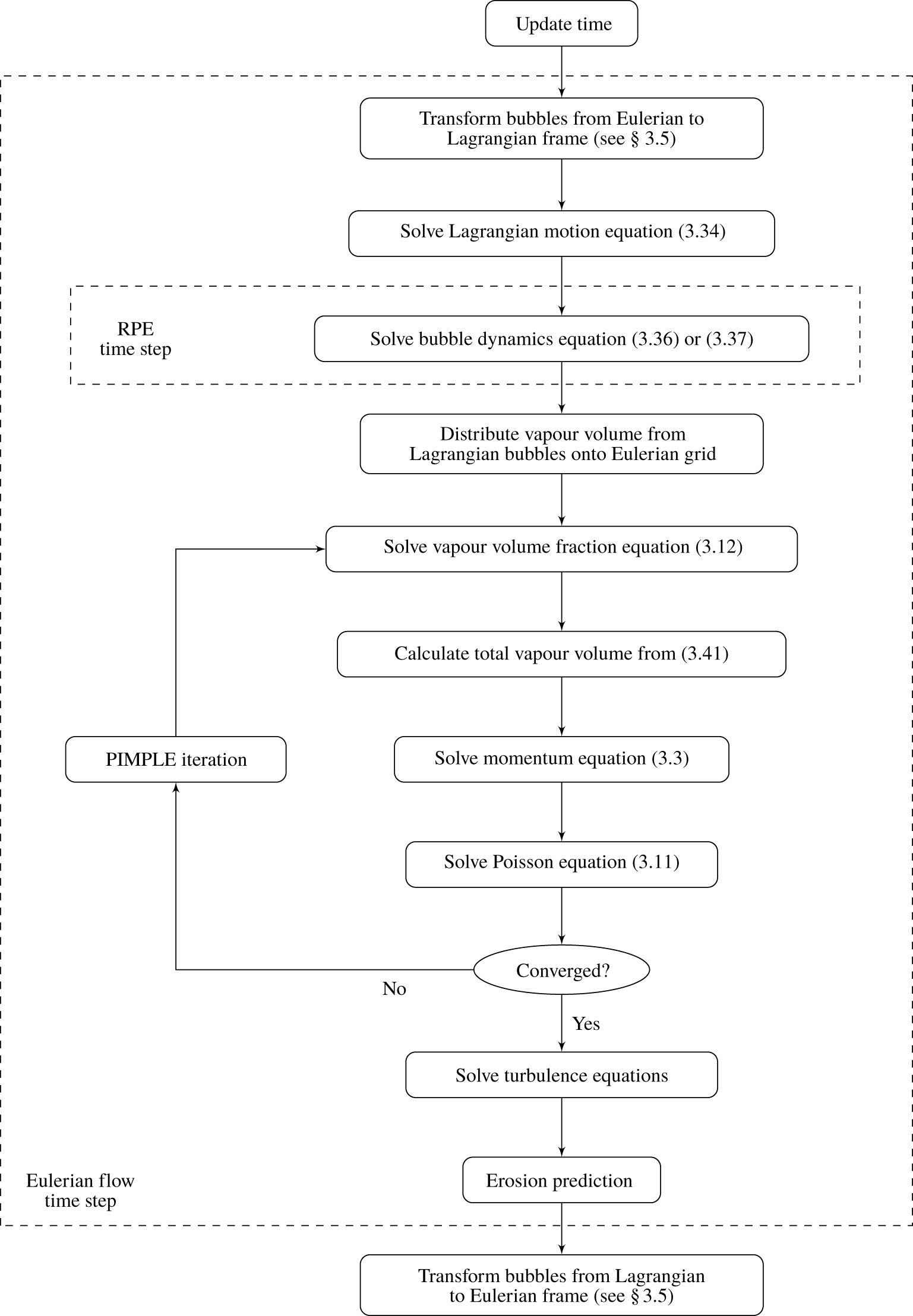
Figure 10. Schematic of the solution algorithm.
Figure 10 schematically outlines our solution algorithm. At the beginning of every time step of the Eulerian flow solution, Eulerian vapour structures, which meet the criteria described in § 3.5, are transformed into spherical Lagrangian bubbles. For every bubble, the Lagrangian equation of motion (3.34) is solved to obtain its new velocity, its position and its source term needed for the momentum equation (3.42). The time step used for the solution of the Lagrange equation equals the time step of the Euler flow solver. Nevertheless, for every bubble we defined a local Courant number based on its velocity relative to the size of the cell incorporating this bubble. Then, if necessary, the time step is reduced, and sub time stepping is conducted over the entire Euler time step.
Solving bubble dynamics equations (3.36) and (3.37) for all bubbles yields bubble radii and their radius growth rates. To track the dynamics of single bubbles which takes place in time periods multiple orders smaller than the time periods considered for the Eulerian flow solution, the time steps used for the integration of  ${\dot{R}}$ and $\ddot{R}$ are significantly smaller. Time integration is conducted using an implicit second-order Crank–Nicolson scheme. Additionally, as growth and collapse take place in different time scales, adaptive time stepping is used for the time integration of bubble dynamics. Then, to estimate erosion, collapse rates of single bubbles near rigid boundaries are stored for post-processing.
Once the size and position of the Lagrangian bubbles are obtained, the new amount of vapour in every control volume is calculated by distribution of the vapour volume onto the numerical grid. Solving equation (3.12) gives the volume fraction for the Eulerian frame, and summing the vapour volume fraction fields from Eulerian and Lagrangian frames (3.41) yields the total vapour volume fraction.
The next steps consist of calculating the velocity and pressure fields of the Eulerian carrier fluid flow by solving the momentum equation (3.3) and the Poisson equation (3.11) in a segregated manner. The PIMPLE algorithm, a combination of the Pressure Implicit with Splitting of Operator (PISO) and Semi-Implicit Method for Pressure-Linked Equations (SIMPLE) algorithms, is used to solve the equations of the Eulerian fluid flow. In contrast to flows without phase change, the solution of the Poisson equation (3.11) differs for cavitating flows because the velocity field is no longer free of divergence. As described above, source terms from the cavitation model account for this divergence. These source terms (3.18) are calculated before solving the Poisson equation to obtain the pressure of the carrier fluid.
If velocities and pressures fail to converge, another outer PIMPLE iteration is initiated. Equations for Eulerian vapour volume fraction, momentum and pressure are solved repetitively until convergence criteria are fulfilled. Then the turbulence equations are solved. If an Eulerian erosion assessment is to be conducted, it is done after completing the flow simulation time step (see § 3.7.1).
Second-order schemes spatially discretise the Euler flow simulations. First-order schemes are used to discretise the turbulence equations to improve numerical stability. An implicit Euler scheme integrates the flow equations.
4 Verification and validation
4.1 Bubble dynamics in an acoustic field
Pressure changes in the surrounding liquid are the main reason for bubble dynamics to be initiated. Before investigating agglomerations of multiple moving bubbles in a flow, we examined the dynamics of a single static bubble based on the experimental measurements of Ohl et al. (Reference Ohl, Kurz, Geisler, Lindau and Lauterborn1999). We considered a bubble in equilibrium at a radius of  $R_{0}=8~\unicode[STIX]{x03BC}\text{m}$ and at atmospheric pressure of $p_{0}=100~\text{kPa}$. An acoustic wave of a frequency of $f_{ac}=21.4~\text{kHz}$ and an acoustic pressure of $p_{ac}=132~\text{kPa}$ prescribed a liquid pressure field.
To illustrate our numerical predictions of bubble dynamics, figure 11(a) presents time histories of the measured and calculated radius of a bubble exposed to an acoustic pressure wave, and figure 11(b) depicts time histories of the radius and the inner pressure of the bubble. In figure 11(a), the black line identifies calculated radii; the red crosses, comparative experimentally measured radii; the blue line, the prescribed acoustic pressure. These time histories were shifted to visualise the instance when liquid and atmospheric pressure were equal. At the beginning, the bubble radius started to grow because liquid pressure decreased below atmospheric pressure, at which the bubble was initially in equilibrium. The bubble growth rate reached its maximum approximately when the acoustic pressure was minimal. When the liquid pressure started to grow again, the acceleration of the bubble wall became negative and caused the bubble’s growth rate to decrease. Further bubble growth led to a decrease of the bubble’s inner pressure, and this inner pressure approached the vapour pressure until the bubble attained its maximum radius. When the liquid pressure exceeded the atmospheric pressure again, it initiated the first bubble collapse. As the non-condensable gas inside the bubble was compressed the bubble’s radius decreased well below its equilibrium radius.
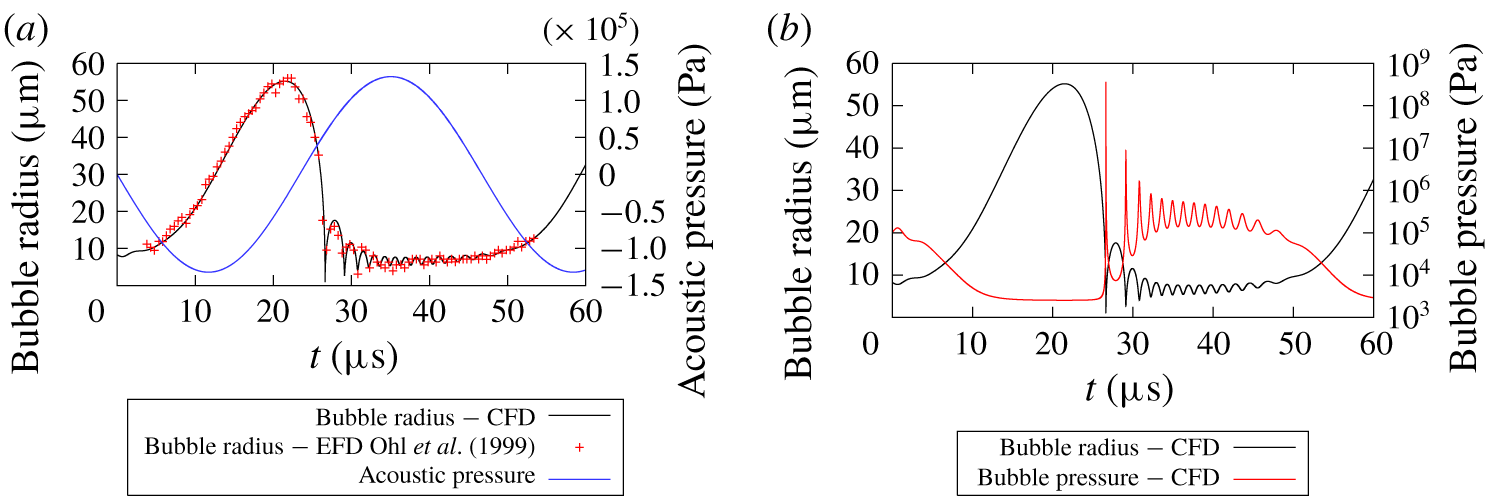
Figure 11. Dynamics of a spherical cavitation bubble exposed to an acoustic wave. (a) Time histories of measured and calculated radius of a spherical cavitation bubble exposed to an acoustic wave in an infinite liquid. (b) Time histories of calculated radius and inner pressure of a spherical cavitation bubble exposed to an acoustic wave in an infinite liquid.
At the end of the collapse, the pressure inside the bubble increased by multiple orders of magnitude above the equilibrium pressure. The peak of the red line in the right graph of figure 11(a) visualises the process, which is in accordance with an adiabatic change of state of an ideal gas. During collapse, the largest part of the potential energy, which was stored in the bubble at maximum size, was converted into energy to form shock waves that were radiated into the liquid. Viscous effects dissipated additional energy. Compression and expansion of the non-condensable gas caused multiple bubble radius and pressure oscillations of decreasing amplitude. The entire process was repeated periodically according to the frequency of the acoustic pressure oscillation. Calculated and measured radii compared favourably.
4.2 Behaviour of a bubble in a vortex
To ensure that a single bubble’s motion and the associated dynamics were calculated correctly and interacted reasonably with each other, using a one-way coupling approach, we simulated the behaviour of a spherical bubble in a Lamb–Oseen-based vortex flow based on the work of Oweis et al. (Reference Oweis, van der Hout, Iyer, Tryggvason and Ceccio2005). Chahine (Reference Chahine1995) and Choi et al. (Reference Choi, Hsiao, Chahine and Ceccio2009) documented more complex investigations of bubbles captured by vortices to account for bubble–vortex interactions and aspherical bubble deformations. Generally, vortex flows can be modelled as Rankine vortices, consisting of the combination of the following two vortex parts:
(i) a rotational vortex (with: $\unicode[STIX]{x1D735}\times \boldsymbol{u}\neq 0$; rigid body vortex) on the inside ($r<r_{c}$); and
(ii) an irrotational vortex (with:
$\unicode[STIX]{x1D735}\times \boldsymbol{u}=0$) on the outside ($r\geqslant r_{c}$).


The two vortex parts are joined at the core radius,  $r_{c}$, measured from the centre of its rotational axis. At the vortex core, the tangential velocity is greatest and is calculated as follows:
 $$\begin{eqnarray}u_{c}=\unicode[STIX]{x1D6FE}_{1}\frac{\unicode[STIX]{x1D6E4}_{0}}{2\unicode[STIX]{x03C0}r_{c}}.\end{eqnarray}$$
The corresponding core pressure is defined as
 $$\begin{eqnarray}p_{c}=p_{\infty }-\frac{\unicode[STIX]{x1D70C}_{l}}{2}u_{c}^{2}.\end{eqnarray}$$
 Here,  $\unicode[STIX]{x1D6E4}_{0}=0.29~\text{m}^{2}~\text{s}^{-1}$ is the circulation of the vortex and $\unicode[STIX]{x1D6FE}_{1}=0.715$. $p_{\infty }$ is the pressure in the undisturbed far field. The tangential velocity measured from the centre of the vortex axis of rotation reads as follows:
 $$\begin{eqnarray}u_{\unicode[STIX]{x1D703}}=\unicode[STIX]{x1D6FE}_{1}\frac{\unicode[STIX]{x1D6E4}_{0}}{2\unicode[STIX]{x03C0}r_{c}}\frac{r}{r_{c}}.\end{eqnarray}$$
 It increases with increasing radius,  $r$, from $0~\text{m}~\text{s}^{-1}$ at the vortex centre to its maximum value, $u_{c}$, at the vortex core. The pressure inside the inner rotational vortex region is defined as follows:
 $$\begin{eqnarray}p=p_{c}+\unicode[STIX]{x1D6FE}_{2}\unicode[STIX]{x1D70C}_{l}\left(\frac{\unicode[STIX]{x1D6E4}_{0}}{2\unicode[STIX]{x03C0}r_{c}}\right)^{2}\frac{(r^{2}-r_{c}^{2})}{r_{c}^{2}},\end{eqnarray}$$
 with  $\unicode[STIX]{x1D6FE}_{2}=0.87$. Outside the vortex core ( $r\geqslant r_{c}$), the flow velocity decreases with increasing distance from the vortex core
 $$\begin{eqnarray}u_{\unicode[STIX]{x1D703}}=\frac{\unicode[STIX]{x1D6E4}_{0}}{2\unicode[STIX]{x03C0}r_{c}}(1-e^{-\unicode[STIX]{x1D6FE}_{3}(r/r_{c})^{2}}),\end{eqnarray}$$
 where  $\unicode[STIX]{x1D6FE}_{3}=1.255$. The pressure, $p$, increases with increasing distance from the centre of the vortex axis of rotation. It is calculated by substituting equation (4.5) into the following expression:
 $$\begin{eqnarray}p=p_{\infty }-\frac{\unicode[STIX]{x1D70C}_{l}}{2}u_{\unicode[STIX]{x1D703}}^{2}.\end{eqnarray}$$
 For vortex flows, the cavitation number at the vortex core can be defined using the vortex core pressure,  $p_{c}$, the vapour pressure, $p_{v}$, and the core velocity, $u_{c}$ (Choi et al. Reference Choi, Hsiao, Chahine and Ceccio2009)
 $$\begin{eqnarray}\unicode[STIX]{x1D70E}_{c}=\frac{p_{c}-p_{v}}{0.5\unicode[STIX]{x1D70C}_{l}{u_{c}}^{2}}.\end{eqnarray}$$
By changing the pressure difference, the bubble dynamics is influenced without changing the flow field of the vortex.

Figure 12. Specified distributions of velocity (a) and pressure (b) for the vortex.
Figure 12 depicts the velocity and pressure distributions for the vortex. Arrows in figure 12(a) identify magnitude and direction of the counter-clockwise flow. Flow velocities were highest near the vortex core and decreased with increasing distance away from the vortex core. Varying colours in figure 12(b) mark the corresponding pressure. They are seen to increase with increasing distance from the vortex rotation axis.
According to Ligneul & Latorre (Reference Ligneul and Latorre1989), for bubbles captured by vortices, a ratio,  $N$, can be defined to describe the influence of forces attracting the bubble towards the vortex centre and forces keeping the bubble in a rotational motion. It is written as follows:
 $$\begin{eqnarray}N=R_{a}\frac{L_{i}}{R_{a}},\end{eqnarray}$$
 where the parameter  $R_{a}$ is calculated as follows:
 $$\begin{eqnarray}R_{a}=\sqrt{\frac{6\unicode[STIX]{x03C0}\unicode[STIX]{x1D708}}{\unicode[STIX]{x1D6E4}_{0}}}=8\times 10^{-3}.\end{eqnarray}$$
 For  $N\approx 1.0$, attractive and rotational forces are of the same order of magnitude; for $N<1.0$, attractive forces increase; for $N>1.0$, rotational forces increase. For the smallest bubble radius of $R_{0}=0.8~\text{mm}$, this ratio is $N=2.52$; for $R_{0}=2~\text{mm}$, $N=1.01$; for $R_{0}=5~\text{mm}$, $N=0.4$.
Bubbles with nucleus radii of  $R_{0}=0.8$, 2.0 and 5.0 mm were initially placed a radial distance of $L_{i}=0.25~\text{m}$ away from the vortex rotational axis, here with a vortex core radius of $r_{c}=0.1~\text{m}$. At first, we specified a core cavitation number of $\unicode[STIX]{x1D70E}_{c}=3.602$. To compute bubble motions, forces caused by the pressure gradient (3.24), virtual mass (3.25), volume variation (3.26), drag (3.27) and lift (3.30) were considered. Initially, the bubble velocity equalled the carrier fluid velocity, causing the bubble to move in a rotational counter-clockwise direction along the streamlines of the flow. Thereafter, the bubble’s trajectory deviated from the carrier flow streamlines as multiple forces influenced its motions.
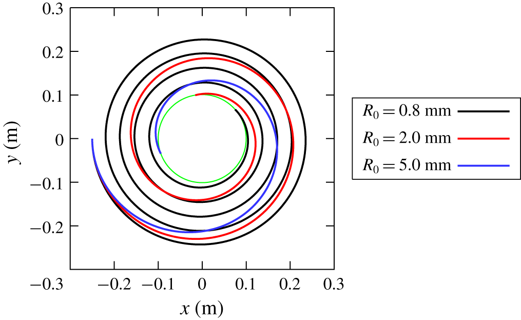
Figure 13. Influence of initial bubble radius on bubble trajectories in a vortex.
Figure 13 presents the trajectories for bubbles of different radii inside the vortex. The bubbles’ starting position was located at  $x=-0.25~\text{m}$ and $y=0~\text{m}$. A green circle marks the vortex core radius, $r_{c}$. The attractive forces towards the vortex core were greatest for the largest bubble. While the bubble of radius $R_{0}=0.8~\text{mm}$ circled around the vortex core for more than four rotations before reaching the core radius, the bubble of radius $R_{0}=5~\text{mm}$ reached the core radius after just one rotation.
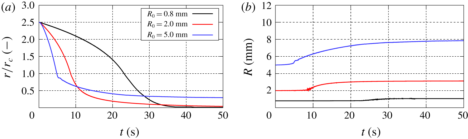
Figure 14. Influence of initial bubble radius on bubble motion in terms of radial distance to the vortex centre (a) and the bubble dynamics (b).
Figure 14(a) depicts the normalised radial distance,  $r/r_{c}$, ( $r$ is the absolute radial distance, and $r_{c}$ is the vortex core radius) of the bubble’s centre to the rotational axis of the vortex; figure 14(b), the bubble radius, $R$, for different initial bubble radii, $R_{0}$. Depending on bubble size and bubble dynamics, forces acting on the path of the bubble increased or decreased. Although all bubbles were attracted to the vortex core, the attractive forces increased with increasing $R_{0}$ and with decreasing $N$, which agreed favourably with the findings of Levkovskii (Reference Levkovskii1978), Latorre (Reference Latorre1980) and Ligneul & Latorre (Reference Ligneul and Latorre1989). Specifically, the pressure gradient forces caused the bubbles to be attracted towards the vortex centre, where the pressure was lowest. Because the liquid pressures around the bubbles’ walls were averaged over multiple locations, the bubbles’ centres did not move into the vortex centre. According to Hsiao et al. (Reference Hsiao, Chahine and Liu2000) and Hsiao et al. (Reference Hsiao, Chahine and Liu2003), this approach can prevent unrealistic bubble growth inside a vortex core. Figure 14(b) presents the dynamics of three bubbles. All three bubbles grew, reached a new equilibrium radius, and followed a trajectory around the vortex. Recall that, in this simplified one-way coupling simulation, although the bubble was influenced by the flow field, the flow field itself was not influenced by the bubble.

Figure 15. Influence of cavitation number,  $\unicode[STIX]{x1D70E}$, on bubble motion in terms of radial distance to the vortex centre (a) and the bubble dynamics (b).
Figure 15(a) presents the normalised radial distance,  $r/r_{c}$, extending from the bubble centre to the rotation axis of the vortex; figure 15(b), the bubble radius, $R$, for core cavitation numbers of $\unicode[STIX]{x1D70E}_{c}=2.682$, 3.142 and 3.602. In all cases, bubbles were attracted to the vortex core and grew until they oscillated about their equilibrium sizes. For smaller cavitation numbers, not only the size of the bubbles, but also the amplitudes of their size oscillations increased. Averaging the liquid pressure at the bubbles’ walls prevented an unbounded growth. The simulated bubble behaviour was similar to that of Hsiao et al. (Reference Hsiao, Chahine and Liu2003), who used a related approach to investigate a spherical single bubble in a vortex.
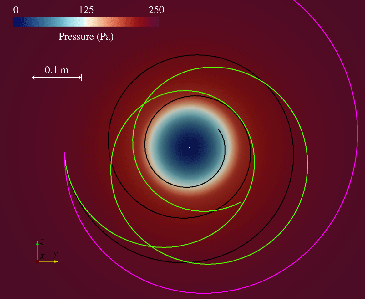
Figure 16. Simulated bubble trajectories considering all forces (black line), forces without drag force (green line) and forces without the pressure gradient force (pink line).
In hydrodynamic flows, two dominant forces mostly define a bubble’s motion, namely the drag force and the pressure gradient force. To visualise their effect, figure 16 shows three simulated trajectories of the bubble’s motion. All three simulations started with the same sized bubble of  $R_{0}=2~\text{mm}$ located at the same position. At the start, the bubble’s velocity equalled the carrier fluid velocity of the control volume incorporating the bubble initially. The black line identifies the bubble’s trajectory considering all forces; the green line, the bubble’s trajectory considering all forces except the drag force, (3.27); the pink line, the bubble’s trajectory considering all forces except the pressure gradient force, (3.24). The pressure gradient force mainly caused the bubble to move to low pressure regions, i.e. towards the vortex centre, where the fluid pressure was lowest. By neglecting this force, the bubble mostly followed streamlines of the carrier fluid flow (pink line in figure 16). The importance of the drag force is clearly obvious, too. By neglecting the drag force, the bubble deviated from streamlines of the carrier fluid as its motion was then dominated by the pressure gradient force, causing it to move towards the centre of the vortex (green line in figure 16). This oscillatory behaviour was additionally influenced by forces that depend on bubble dynamics. Considering both the drag and the pressure gradient force, the bubble approached the vortex centre following a spiral-shaped path (black line in figure 16).
4.3 Bubble rising in a liquid column
Gas bubbles rise in resting liquids owing to the gravity or buoyancy force generated by the density difference between the gas inside a bubble and the liquid surrounding this bubble. After an initial acceleration, a rising bubble reaches its final rise velocity because an equilibrium between buoyancy force and drag force is achieved. An analytical solution yields the final rise velocity of the bubble.
Based on a bubble’s interaction with the liquid phase, we employed a one-way and a two-way coupling technique to simulate a bubble rising in a liquid medium initially at rest ( $u_{z}=0~\text{m}~\text{s}^{-1}$). We considered a gas bubble, positioned at the bottom of a water column, having an initial radius of $R_{0}=2~\text{mm}$ and an initial velocity of $u_{b,z}=0~\text{m}~\text{s}^{-1}$. Densities of air and water were assumed to be $\unicode[STIX]{x1D70C}_{air}=1~\text{kg}~\text{m}^{-3}$ and $\unicode[STIX]{x1D70C}_{air}=1000~\text{kg}~\text{m}^{-3}$, respectively. Surface tension of water was set at $\unicode[STIX]{x1D70E}=0.073~\text{N}~\text{m}^{-1}$. For the calculation of bubble motions from the Lagrangian equation, we considered forces owing to gravity (3.32), pressure gradient (3.24), virtual mass (3.25), Saffman lift (3.30), and drag attributable to gravity (3.29).
Assuming that buoyancy and gravity forces are in equilibrium and that no other forces influence the bubble’s motion, Darmana et al. (Reference Darmana, Deen and Kuipers2006) derived the following analytical formula for the bubble’s final rise velocity:
 $$\begin{eqnarray}u_{b,z}=u_{z}+\sqrt{\frac{\unicode[STIX]{x1D70E}}{R\unicode[STIX]{x1D70C}_{c}}+\frac{(\unicode[STIX]{x1D70C}_{c}-\unicode[STIX]{x1D70C}_{b})|g_{z}|R}{\unicode[STIX]{x1D70C}_{c}}}.\end{eqnarray}$$
 Under initial conditions and fluid properties mentioned above, a final rise velocity of  $u_{b,z}=0.23686~\text{m}~\text{s}^{-1}$ is obtained.
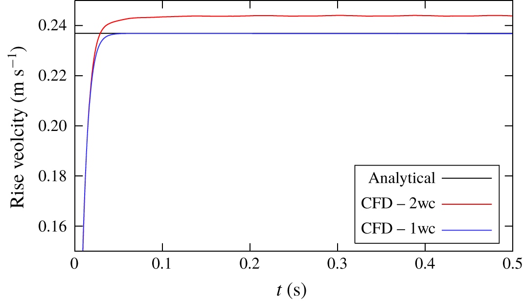
Figure 17. Rise velocity of the bubble obtained from an analytical calculation and from simulations employing one-way (CFD – 1wc) and two-way coupling techniques (CFD – 2wc).
Figure 17 depicts the rise velocities of a bubble obtained from the analytical solution and from simulations applying one-way and two-way coupling. In this figure, the black line marks the analytical solution; the blue line, the simulated time history from the one-way coupling technique; the red line, the simulated time history from the two-way coupling technique. Our simulations predicted that the initially resting bubble accelerated, causing the rise velocity obtained from the one-way coupling technique to asymptotically approach the analytical solution, thereby correctly verifying the numerical solution of the Lagrangian equation of motion. However, from the two-way technique we obtained a rise velocity that was approximately 3 % higher than the analytical solution. This apparent discrepancy was attributed to the upward motion of the bubble, which transferred its momentum to the surrounding liquid. Consequently, the liquid surrounding the bubble was also accelerated, thereby decreasing the bubble’s relative velocity and reducing the drag force acting on the bubble.
4.4 Coalescence of a Lagrangian bubble with an Eulerian vapour structure
To demonstrate the ability of our hybrid approach to transform a vapour volume from the Lagrangian to the Eulerian framework and vice versa, we simulated the process to merge a small Lagrangian bubble with a larger almost spherical vapour structure in the Eulerian framework. To visualise this transformation between frames, we deactivated the solution of the equations of bubble motion and bubble dynamics for the Lagrangian bubbles. The velocity of the Lagrangian bubble was predefined, such that it moved with constant velocity in the direction of the Eulerian vapour structure.
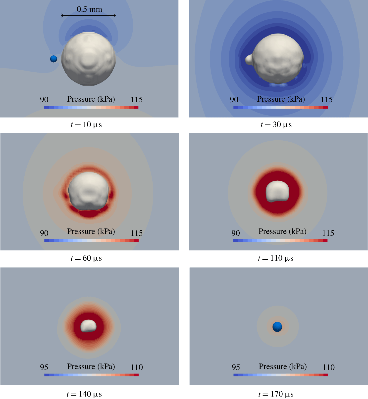
Figure 18. Coalescence of a single Lagrangian bubble with an Eulerian vapour volume, the collapse of the Eulerian vapour volume and the vapour volume’s subsequent transformation into a Lagrangian bubble.
Figure 18 illustrates the coalescence of a spherical Lagrangian bubble (identified by a small blue coloured sphere) with an Eulerian vapour volume (distinguished by a grey coloured shape) followed by the collapse of this Eulerian vapour volume and its subsequent transformation into a Lagrangian bubble. At time  $t=10~\unicode[STIX]{x03BC}\text{s}$, the Lagrangian bubble approached the Eulerian vapour structure and coalesced with it at time $t=30~\unicode[STIX]{x03BC}\text{s}$. Then, the complete vapour volume of the Lagrangian bubble was transformed into the Eulerian frame. The influence of the coalesced Lagrangian bubble on the shape of the vapour volume remained until, at time $t=60~\unicode[STIX]{x03BC}\text{s}$, the Eulerian vapour structure began to collapse because the pressure surrounding the bubble greatly exceeded the vapour pressure. Furthermore, the action of gravity caused the bubble to deform asymmetrically in the vertical direction. Between times $t=140~\unicode[STIX]{x03BC}\text{s}$ and $t=170~\unicode[STIX]{x03BC}\text{s}$, the Eulerian volume was transformed into a spherical Lagrangian bubble because the vapour volume decreased below the threshold volume related to the predefined bubble’s limit radius of $R_{limit}=50~\unicode[STIX]{x03BC}\text{m}$.
5 Cavitation in internal nozzle flow
Following the work of Peters et al. (Reference Peters, Lantermann and el Moctar2015a,Reference Peters, Sagar, Lantermann and el Moctarb), we used a RANS approach to simulate the flow passing through an axisymmetric vertical nozzle, subjecting a target plate to cavitation erosion. Franc & Riondet (Reference Franc and Riondet2006) and Franc et al. (Reference Franc, Riondet, Karimi and Chahine2011) investigated the internal nozzle flow experimentally with regard to erosion damage caused by cavitation. Mihatsch et al. (Reference Mihatsch, Schmidt, Thalhamer, Adams, Skoda and Iben2011), Koukouvinis, Bergeles & Gavaises (Reference Koukouvinis, Bergeles and Gavaises2014), Mihatsch, Schmidt & Adams (Reference Mihatsch, Schmidt and Adams2015) and Mottyll (Reference Mottyll2017) numerically assessed cavitation erosion for the considered case. Figure 19 shows the geometry of the nozzle configuration we analysed. The nozzle consisted of a 16 mm diameter vertical cylinder and a horizontal target plate, which formed the bottom of a 2.5 mm high diverging radial channel. With an average velocity of  $31~\text{m}~\text{s}^{-1}$ the flow passed through the nozzle and, at the connection of the nozzle with this channel, the small radius of only 1.0 mm ensured that flow separated and then accelerated, generating transient sheet and cloud cavitation travelling downstream on the target plate until collapsing in regions of higher pressure. The high outlet pressure of the channel of 10.1 bar caused aggressive cavitation collapses leading to erosion on the target plate (Franc & Riondet Reference Franc and Riondet2006; Franc et al. Reference Franc, Riondet, Karimi and Chahine2011). The greatest erosion occurred within a radial distance of approximately 21 to 22 mm from the nozzle’s central axis.
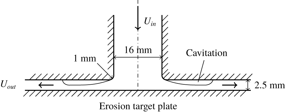
Figure 19. Sketch of the nozzle’s geometry (Peters et al. Reference Peters, Sagar, Lantermann and el Moctar2015b).
To reduce computational costs, the numerical grid we constructed for our simulations encompassed a three-dimensional symmetrical  $17.5^{\circ }$ section of the nozzle’s flow domain as shown in figure 20. In the radial direction, control volumes were slowly growing to obtain the highest spatial resolution near the radius where cavitation structures were generated. Furthermore, cell sizes near solid surfaces were specified in accordance with dimensionless wall distances, $n^{+}$, to enable the use of logarithmic wall functions. The inlet boundary was located at a height of 50 mm above the connecting radius; the outlet, a radius of 100 mm from the centre axis of the nozzle. No-slip velocity conditions were specified for the outer cylinder and the top and bottom boundaries of the diverging radial channel. Periodic boundary conditions were defined for the side boundaries whose normal vectors pointed in circumferential direction. All cases were simulated for a time of at least 0.25 s which represents over 80 periods associated with the lowest identified shedding frequency of approximately 350 Hz and enabled us to calculate a sufficient number of Lagrangian collapses in the vicinity of the target surface. We relied on an implicit Euler scheme to perform time integrations of the flow solution. To obtain a maximum Courant number of less than two and an average Courant number of approximately $2.5\times 10^{-3}$, a time step of $\unicode[STIX]{x0394}t=3.54\times 10^{-7}~\text{s}$ was specified. A first-order upwind scheme spatially discretised convective turbulence terms; second-order schemes, all other terms. To model cavitation for vapour structures treated in the Eulerian frame, the cavitation model by Sauer & Schnerr (Reference Sauer and Schnerr2000) with a nuclei density of $n_{0}=1\times 10^{11}~\text{m}^{-3}$ was used. To model turbulence, we used the $k$–
$k$– $\unicode[STIX]{x1D714}$-SST model together with the correction of turbulent kinetic energy proposed by Reboud et al. (Reference Reboud, Stutz and Coutier-Delgosha1998) (see (3.19), (3.20)). To calculate the dynamics of spherical bubbles, we used equations (3.36) and (3.37) and an adaptive time-stepping technique to deal with relatively long growth and relatively short collapse phases. The time loop for the bubble dynamics was integrated until reaching the next time step of the Eulerian flow solution. To compute bubble motions, forces owing to pressure gradient, (3.24), virtual mass, (3.25), volume variation, (3.26), drag, (3.27), lift, (3.30) and gravity, (3.32) were considered. Lagrangian bubbles introduced into the simulation by the transformation mechanisms interacted with the carrier fluid via a two-way coupling approach.
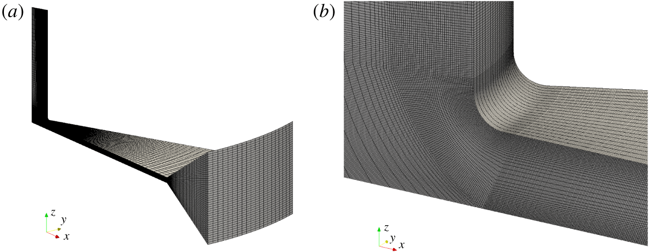
Figure 20. Perspective view of the entire solution domain (a) and a detailed view of the small radius region of cavitation inception (b).
First, the flow passing through the nozzle was computed using pure Euler–Euler simulations. Figure 21 shows a time instance of the circumferential cross section of the rotationally symmetric nozzle geometry for this Euler–Euler simulation. The left half plots the velocity magnitude; the right half, the pressure inside the domain. The flow from the top to the bottom caused a stagnation point flow at the bottom boundary of the domain. At the stagnation point, the pressure was of a magnitude of approximately 20 bar. Downstream of the 1 mm radius, which connected the top cylinder to the radial divergent part, the flow accelerated into the channel, and vortices were generated. In the vicinity of the radius, the pressure decreased, reaching values lower than the vapour pressure, so that cavitation structures grew, which travelled radially outwards. Further downstream, the static pressure increased again, leading to collapsing cavitation structures.

Figure 21. Circumferential cross-section of the nozzle domain showing the velocity magnitude on the left half and the pressure on the right half.
We performed Euler–Euler simulations on seven grids consisting of  $8.90\times 10^{4}$ to $2.09\times 10^{6}$ control volumes. A refinement ratio of $2^{1/4}$ between the edge lengths of consecutive grids in all three directions was specified. Based on calculations obtained on these seven grids, figure 22(a) plots time-averaged normalised vapour volume in the computational domain ( $\overline{V}_{v}^{\ast }=\overline{V}_{v}/V_{dom}$) versus refinement ratio of each grid relative to the coarsest grid ( $r$).
$r$).  $V_{v}$ is the time-averaged volume of vapour in the numerical domain and $V_{dom}$ is the volume of the entire domain. The coarsest grid is denoted as $r=1$ and the finest grid as $r=2\sqrt{2}$. The vapour volume on grid $r=2$ deviated by $-$1 % relative to the vapour volume calculated on the finest grid $r=2\sqrt{2}$.
Figure 22(b) plots the relative deviation of the number of exceedances of vertical force acting on the bottom boundary of the domain relative to the number of exceedances obtained on the finest grid  $r=2\sqrt{2}$. The relative deviation of the number of exceedances obtained on grid $i$ relative to the finest grid was calculated as $\unicode[STIX]{x1D716}_{N_{F},i}=(N_{F,i}-N_{F,fine})/N_{F,fine}$. Here, $N_{F,i}$ is the number of exceedances of vertical force obtained on grid $i$ and $N_{F,fine}$ is the number of exceedances of vertical force obtained on the finest grid. $F_{Z}/F_{0}$ is the vertical force on the bottom boundary, $F_{Z}$, normalised against $F_{0}=-25~\text{kN}$. Increasing the refinement, $r$, caused deviations of calculated forces to decrease smaller.
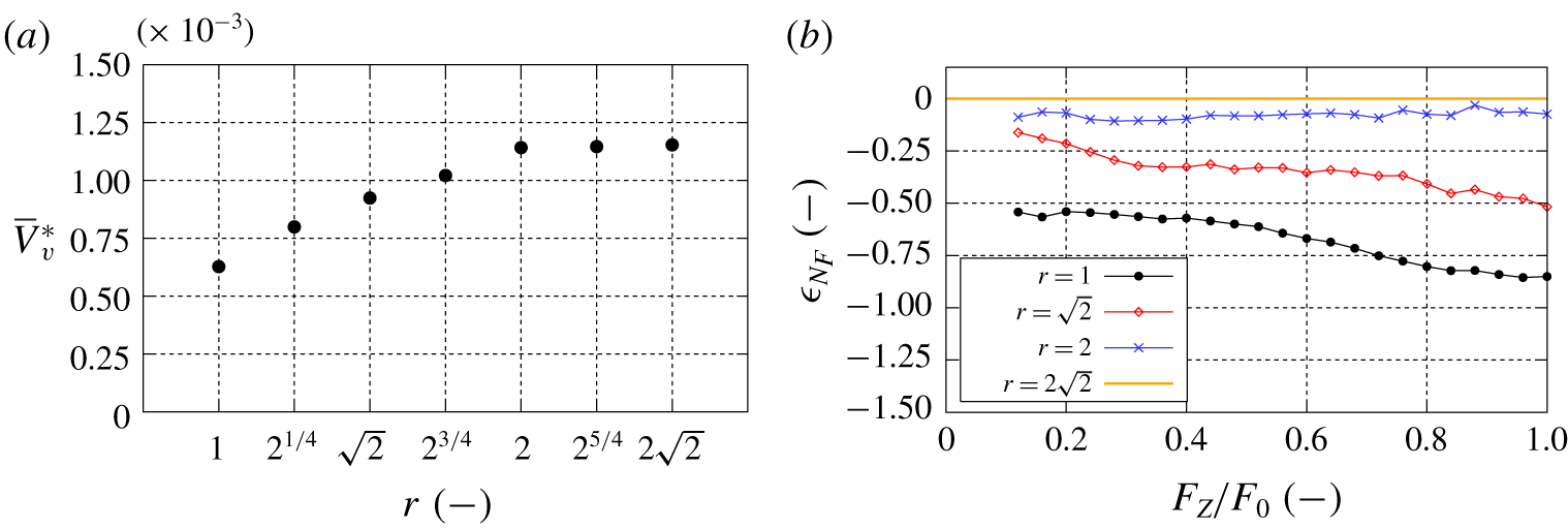
Figure 22. Time-averaged normalised vapour volume in the domain,  $\overline{V}_{v}^{\ast }$, versus the refinement ratio of each grid, relative to the coarsest grid, $r$, (a) and relative deviation of exceedances of vertical force acting on the bottom boundary, relative to the one obtained on the finest grid, $\unicode[STIX]{x1D716}_{N_{F},i}=(N_{F,i}-N_{F,fine})/N_{F,fine}$ (b). $N_{F,i}$ is the number of exceedances of vertical force obtained on grid $i$ and $N_{F,fine}$ is the number of exceedances of vertical force on the finest grid. $F_{Z}/F_{0}$ is the vertical force acting on the bottom boundary, $F_{Z}$, normalised against $F_{0}=-25~\text{kN}$.
On a double logarithmic scale, figure 23 plots the amplitude of  $V_{v}^{\ast }$ versus the frequency. Although a seemingly unsteady behaviour characterised the temporal progression and shape of the vapour volume, the fast Fourier transform (FFT) of simulations on grids $r=\sqrt{2}$, $r=2$ and $r=2\sqrt{2}$ yielded periodic processes. These identified the first characteristic frequency occurring between 300 and 400 Hz ( $f_{1}\approx 350~\text{Hz}$); the second characteristic frequency, at about $f_{2}\approx 1050~\text{Hz}$; the first harmonic mode of the second characteristic frequency, at approximately $f_{3}\approx 2100~\text{Hz}$. To investigate the effects of the nuclei density, $n_{0}$, on the cavitation characteristics, we performed simulations based on the cavitation model of Sauer & Schnerr (Reference Sauer and Schnerr2000) using nuclei densities of $1\times 10^{8}$, $1\times 10^{11}$, and $1\times 10^{14}~\text{m}^{-3}$, in the cavitation model of Sauer & Schnerr (Reference Sauer and Schnerr2000). For all three nuclei densities, the computed normalised vapour volume in the domain deviated by a maximum of 1.5 %. Further on, the frequency analyses revealed the same characteristic frequencies. Hence, we selected a nuclei density of $n_{0}=1\times 10^{11}~\text{m}^{-3}$ for further investigations.
Mihatsch et al. (Reference Mihatsch, Schmidt, Thalhamer, Adams, Skoda and Iben2011) investigated this case numerically, using a compressible density-based solver that incorporated a barotropic cavitation model. They identified characteristic frequencies of cavitation shedding at 408 Hz and two well-defined frequencies at 1139 and 1182 Hz. Mihatsch et al. (Reference Mihatsch, Schmidt and Adams2015) obtained four dominant frequencies for the same case (denoted as ‘20 bar case’ owing to the stagnation pressure of the incoming flow). They obtained the two lowest frequencies at 350 Hz, a second characteristic frequency at 1100 Hz, and the first harmonic mode of the second characteristic frequency at about 2200 Hz. The frequencies obtained by Mihatsch et al. (Reference Mihatsch, Schmidt, Thalhamer, Adams, Skoda and Iben2011, Reference Mihatsch, Schmidt and Adams2015) agreed favourably with the frequencies we obtained from our simulations. On grid  $r=2$ we were able to capture the dynamic behaviour of cavitation. This enabled us to determine the average amount of vapour in the computational domain and to obtain a favourable agreement between vertical forces acting on the bottom boundary. Therefore, our computations on grid $r=2$ yielded sufficiently accurate results and a workable compromise for further investigations using the multi-scale approach.
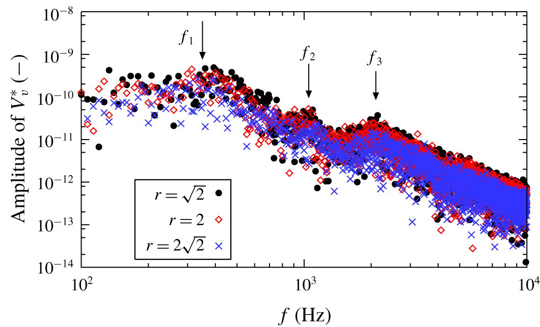
Figure 23. Frequency analysis of the vapour volume calculated on different grids plotted on a double logarithmic scale.
5.1 Hybrid approach – cavitation behaviour
All simulations using the hybrid Euler–Euler/Euler–Lagrange method were started from a previously converged Euler–Euler simulation. Employing our hybrid method to simulate the flow through an axisymmetric vertical nozzle, we united the efficient Eulerian treatment of large vapour structures with the accurate Lagrangian approach and simulated the behaviour of single spherical bubbles. We transformed vapour volumes between the two frames whenever specified conditions as documented above were met (see § 3.5). Specifically, vapour structures were transformed into Lagrangian bubbles when their mesh resolution was too low or their radii decreased below a predefined threshold and, reciprocally, when they grew to a sufficient size or merged with other Eulerian vapour structures.
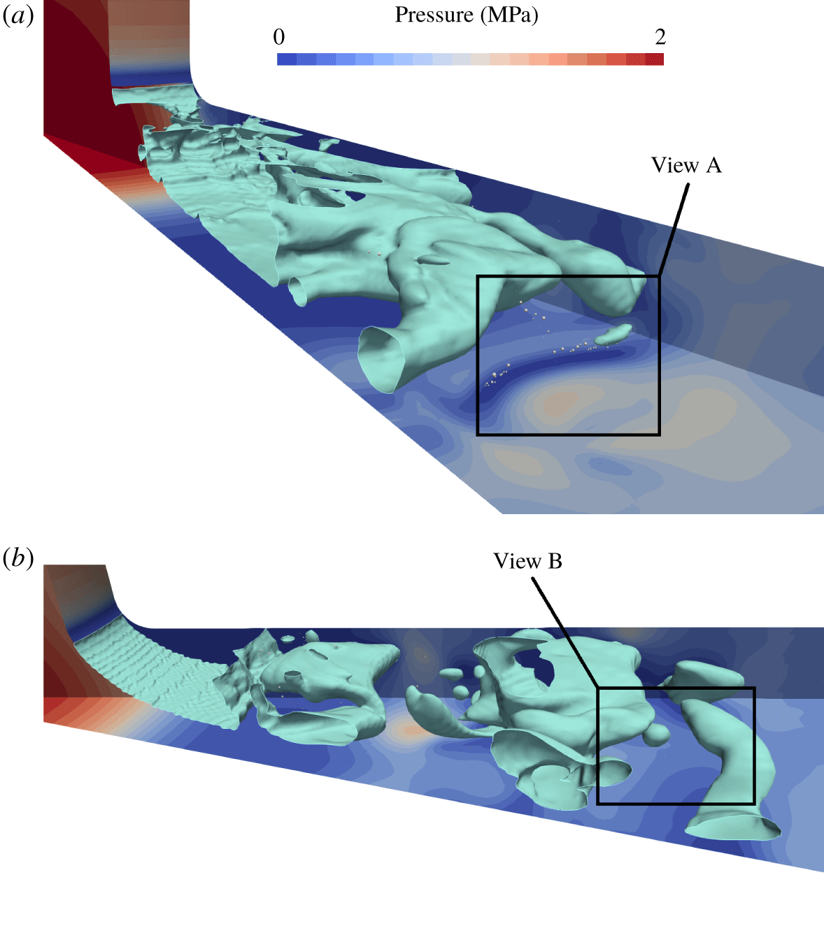
Figure 24. Two perspective views of Eulerian cavitation structures and Lagrangian bubbles at different time instances. See also the supplementary Movie 1 and Movie 2 at https://doi.org/10.1017/jfm.2020.273.
Figure 24 displays two perspective views of larger cavitation structures (light green) and single isolated bubbles (light grey) in the domain at different time instances. Although the domain contained many Lagrangian bubbles, most of them were small until reaching regions of low pressure. At the time instance presented in figure 24(a), single Lagrangian bubbles were introduced owing to vapour structures collapsing or splitting into smaller parts or from the growth of small isolated vapour volumes. Afterwards, bubbles accumulated and started to form a larger vapour structure again. At the time instance shown in figure 24(b), an Eulerian vapour structure detached from a large cavitation cloud, collapsed, and then transformed into a Lagrangian bubble.
Figure 25 illustrates the formation of a large scale vapour structure, starting from individual bubbles (View A from figure 24a). Figure 25  $\unicode[STIX]{x0394}t=0~\unicode[STIX]{x03BC}\text{s}$ to figure 25 $\unicode[STIX]{x0394}t=10.62~\unicode[STIX]{x03BC}\text{s}$ show bubbles that moved to the low pressure region and then grew, while other bubbles followed into this region. At time $\unicode[STIX]{x0394}t=3.54~\unicode[STIX]{x03BC}\text{s}$, bubbles were already large enough to be transformed into the Eulerian framework, and from time $\unicode[STIX]{x0394}t=3.54~\unicode[STIX]{x03BC}\text{s}$ to $\unicode[STIX]{x0394}t=31.86~\unicode[STIX]{x03BC}\text{s}$ Lagrangian bubbles were contacting the Eulerian vapour structure and were consecutively transformed into the Eulerian framework and merged into the larger vapour structure.
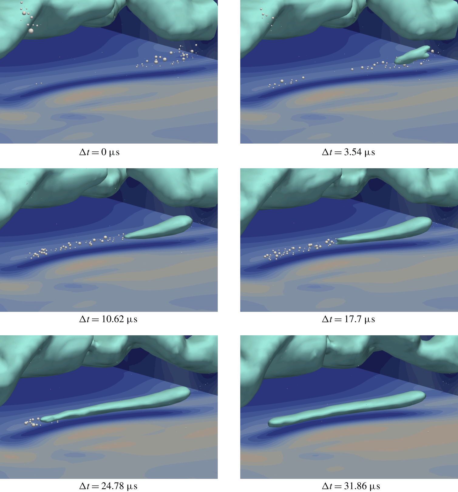
Figure 25. Lagrangian bubbles growing and forming a larger Eulerian vapour structure.
Figure 26 displays the conversion of a vapour volume from the Eulerian into the Lagrangian frame. Starting from the vapour structure shown in View B from figure 24(b), figure 26  $\unicode[STIX]{x0394}t=0~\unicode[STIX]{x03BC}\text{s}$ to figure 26 $\unicode[STIX]{x0394}t=3.54~\unicode[STIX]{x03BC}\text{s}$ present a nearly spherical vapour structure that detached from a large cavitation cloud. Between times $\unicode[STIX]{x0394}t=3.54~\unicode[STIX]{x03BC}\text{s}$ and $\unicode[STIX]{x0394}t=10.62~\unicode[STIX]{x03BC}\text{s}$, after detachment, the vapour volume collapsed. From time $\unicode[STIX]{x0394}t=7.02~\unicode[STIX]{x03BC}\text{s}$ to time $\unicode[STIX]{x0394}t=10.62~\unicode[STIX]{x03BC}\text{s}$, the bubble achieved a size so small that a sufficient resolution by the numerical grid could not be maintained and, therefore, it was transformed into a spherical Lagrangian bubble.

Figure 26. An Eulerian vapour volume detaching from a larger cloud, collapsing and being transformed into a Lagrangian bubble.
Thresholds  $\unicode[STIX]{x1D6FC}_{v,limit}$, $n_{limit}$ and $R_{limit}$ identified those vapour volumes that had to be transformed between the Lagrangian and Eulerian frameworks (see § 3.5). Therefore, we investigated the influence of these thresholds on the transformation processes. Recall that Lagrangian bubbles were transformed into the Eulerian frame, not only owing to growth above a specified threshold ( $n_{limit}$ or $R_{limit}$), but also by merging into present Eulerian vapour structures. Table 1 lists the results of simulations conducted using our hybrid approach, specifically, the number of transformations into the Lagrangian frame per time step, $n_{EtoL}/\unicode[STIX]{x0394}t$, the number of transformations into the Eulerian frame per time step, $n_{LtoE}/\unicode[STIX]{x0394}t$, and the net number of bubbles added into the Lagrangian frame per time step, $\unicode[STIX]{x0394}n/\unicode[STIX]{x0394}t=(n_{EtoL}-n_{LtoE})/\unicode[STIX]{x0394}t$. For simulations H1, H2 and H3, only the threshold $\unicode[STIX]{x1D6FC}_{v,limit}$ varied. Although we found no clear dependence of the number of transformations on $\unicode[STIX]{x1D6FC}_{v,limit}$, its increase yielded a greater net number of bubbles added into the Lagrangian frame per time step, $\unicode[STIX]{x0394}n/\unicode[STIX]{x0394}t$. Simulated cases H2, H4 and H5, differed only in the specified values of threshold $n_{limit}$. With a higher threshold related to the grid resolution, $n_{limit}$, more vapour volumes were transformed from the Eulerian to the Lagrangian frame and vice versa. Nevertheless, the net number of bubbles added into the Lagrangian frame did not show a definite tendency related to the threshold $n_{limit}$. In contrast to the other simulations, case H7 used an absolute threshold radius of $R_{limit}=25~\unicode[STIX]{x03BC}\text{m}$ to evaluate transformations of vapour volumes. Compared to maximum radii achieved in other simulations, this threshold radius was approximately one order smaller. Fewer Eulerian vapour volumes were, therefore, transformed into the Lagrangian frame and a considerably smaller net number of Lagrangian bubbles was introduced. Cases H2, H6 and H8 differed only in the equilibrium radius specified. For simulation H8, the average equilibrium radius was larger than for simulation H2 and it was even larger for simulation H6. Increasing the equilibrium radius yielded a larger number of transformations between the frames in both directions, but decreased their difference per time step, $\unicode[STIX]{x0394}n/\unicode[STIX]{x0394}t$.
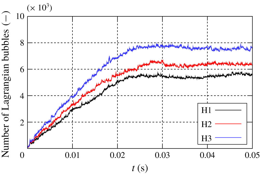
Figure 27. Time history of the total number of Lagrangian bubbles inside the simulation domain for cases H1, H2 and H3.
Table 1. Results of simulations using the hybrid approach with different transformation thresholds.
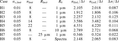
Figure 27 presents the start of the time histories of the total number of Lagrangian bubbles inside the domain for cases H1, H2 and H3. Simulations started from a converged solution of an Euler–Euler simulation. In the beginning, for all cases, the number of Lagrangian bubbles increased until reaching an average number of bubbles at a time of about 0.03 s. This figure shows that the number of Lagrangian bubbles transformed between the two frames and the bubbles moving out of the outlet of the domain approached a value that, depending on the temporal behaviour of cavitation, varied only slightly.
Except for simulation H6, the simulated macroscopic cavitation for the simulations listed in table 1 the simulated macroscopic cavitation behaved similarly compared to an Euler–Euler simulation with regard to the average cavitation volume, its temporal progress, and its characteristic frequencies. These simulations, therefore, were influenced only on a microscopic scale when transforming vapour volumes from the Eulerian frame into the Lagrangian frame. Although we used a Lagrangian approach, which incorporated a two-way coupling technique, to deal with smaller vapour structures, the Lagrangian vapour bubbles correctly replaced the Eulerian vapour volumes and, therefore, did not affect the macroscopic behaviour of cavitation. For simulation H6, we specified a much larger equilibrium bubble radius and, thereby, a greater non-condensable gas content in the bubbles. This resulted in an increased vapour volume in the domain and led to augmented amplitudes of oscillations of the vapour volume. Figure 28 presents time histories of vapour volumes for the Euler–Euler simulation and the H2 and H6 simulations obtained from our hybrid approach. Although the equilibrium radius differed, cases H2 and H6 used the same parameters for the hybrid model (see table 1). The behaviour of macroscopic cavitation was similar for the Euler–Euler simulation and the hybrid simulation H2. For case H6, owing to the high gas content in the bubbles, large oscillations of vapour volume occurred and the average vapour volume increased significantly. For simulation H8, although the gas content in the Lagrangian bubbles was spectrally distributed, the macroscopic cavitation resembled not only the Euler–Euler simulation, but also all other hybrid simulations. The only exception was simulation H6.
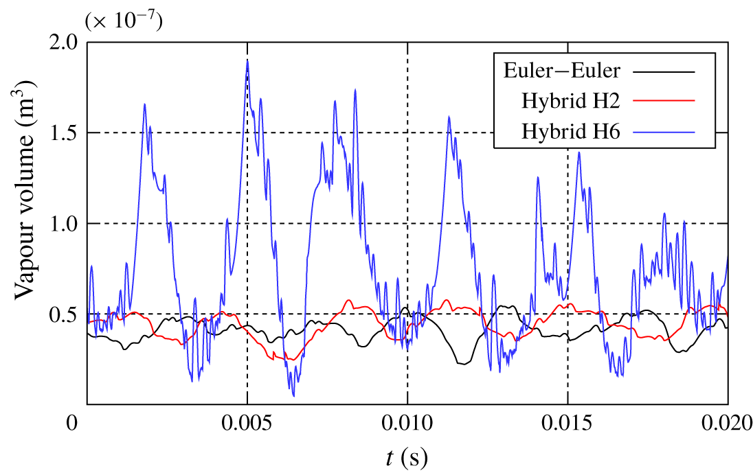
Figure 28. Temporal progress of vapour volume for simulations using an Euler–Euler approach and the hybrid approach for cases H2 and H6.
5.2 Hybrid approach – erosion assessment
To assess erosion caused by the flow through the axisymmetric nozzle, we first identified the bubbles collapsing in the fluid domain and stored their properties, such as collapse pressure, initial and final radii during collapse and bubble position. The procedure then consisted of calculating pressures impacting the rigid target plate. For the dimensionless stand-off distance of  $\unicode[STIX]{x1D6FE}\leqslant 3.0$ of case H4, figure 29(a) visualises Lagrangian bubble collapses impacting on the target plate using their initial bubble radii at the beginning of the respective collapses. In this figure, the blue to red colouring in the domain and a logarithmic scale identify impact pressures, $p_{imp}$, associated with bubble collapses; different shades of grey and another logarithmic scale, the sum of impact pressures on the respective faces, $\sum p_{imp}$. It is seen that a defined region of the target plate is covered by impacts of Lagrangian bubble collapses. In the close-up view, shown in figure 29(b), the darker grey areas identify areas of the target plate subject to erosion by visualising the correlation between erosion potential and bubble collapses. Faces neighbouring collapses of high impact pressures and/or multiple collapses were estimated to have the highest damage potential. Furthermore, bubble collapses for greater stand-off distances ( $\unicode[STIX]{x1D6FE}\geqslant 1.5$) seldom caused high impact pressures.
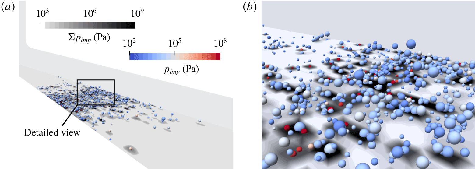
Figure 29. Lagrangian bubble collapses displayed using their maximum radii and sum of impact pressures on the bottom target plate for case H4.
A more quantitative statistical erosion assessment is obtained by evaluation of collapse impacts in circumferential direction of the nozzle at different radial intervals. Franc & Riondet (Reference Franc and Riondet2006) measured the depth of erosion in terms of mass loss on this area of the target plate. Based on an interval length of 1 mm, their moving averaging technique obtained the distribution of penetration depth over the radial distance from the central axis of the nozzle. For comparison purposes, we chose radial intervals of the same length to evaluate Lagrangian collapse impacts. Here, all faces which were multiply impacted were considered. For case H4, figure 30 exemplarily plots the number of impacts (normalised against the maximum number of collapse impacts),  $n_{imp}/n_{imp,max}$, versus the radial distance from the nozzle’s central axis, $r$, obtained for different thresholds of dimensionless collapse distances of $\unicode[STIX]{x1D6FE}\leqslant 1$, $\unicode[STIX]{x1D6FE}\leqslant 3$ and $\unicode[STIX]{x1D6FE}\leqslant 5$. The legend in this figure lists the maximum number of collapse impacts associated with each simulation. Bubbles collapsed mostly between radial distances of 15 to 30 mm. For larger collapse distances, the distribution of calculated impacts turned out to be broader banded and, also, a greater number of impacts were calculated.
To investigate the influence of the parameters listed in table 1 on the simulation of Lagrangian bubble collapses, figure 31 exemplarily plots distributions of the number of impacts per time versus the radial distance from the nozzle’s central axis for  $\unicode[STIX]{x1D6FE}\leqslant 3$ and for cases H1 to H4, case H7 and case H8. Despite small deviations in the distributions’ shapes, in all cases the highest number of impacts was calculated between radial distances of 21 to 22 mm. The number of impacts per unit time increased as $\unicode[STIX]{x1D6FC}_{v,limit}$ and $n_{limit}$ increased and as the average equilibrium radii decreased. Comparing the parameters listed in table 1, it seemed obvious that the number of impacts per unit time increased as $\unicode[STIX]{x1D6FC}_{v,limit}$ from simulation H1 to H2 and from simulation H2 to H3 increased and as $n_{limit}$ from simulation H2 to H4 increased. For simulation H7, the lowest number of calculated impacts correlated well with the fact that, for this case, the number of transformations from Eulerian to Lagrangian vapour volumes, $n_{EtoL}/\unicode[STIX]{x0394}t$, was smallest.
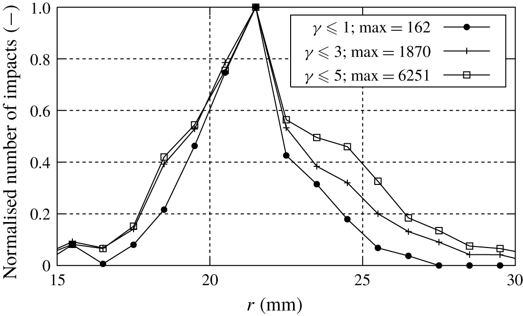
Figure 30. Number of collapses for different collapse distance thresholds versus radial distance from the nozzle’s central axis for case H4.
Franc & Riondet (Reference Franc and Riondet2006) reported that they did not consider pits with diameters smaller than  $20~\unicode[STIX]{x03BC}\text{m}$, because their contribution to overall erosion was too low. The largest pit they found had a diameter of $220~\unicode[STIX]{x03BC}\text{m}$ and characteristic pit diameter leading to most surface erosion was between 80 and $100~\unicode[STIX]{x03BC}\text{m}$. In numerical simulations of single bubbles near a solid wall considering fluid-structure interaction, Chahine (Reference Chahine2014) investigated the dependence of pit radius on the maximum bubble radius at the beginning of a collapse. They found that the radius of a generated pit is similar to the bubble radius at the beginning of a collapse.
More than 95 % of our calculated bubble collapses occurred at maximum diameters between 20 and  $180~\unicode[STIX]{x03BC}\text{m}$ for simulations H1, H2 and H3; for simulation H4, between 20 and $400~\unicode[STIX]{x03BC}\text{m}$; for simulation H7, between 20 and $50~\unicode[STIX]{x03BC}\text{m}$; for simulation H8, between $20~\unicode[STIX]{x03BC}\text{m}$ and 1 mm. Maximum collapse radii were smaller for simulation H7 because the maximum Lagrangian bubble size was limited by the transformation threshold $R_{limit}$ and were larger for simulation H8 because the average equilibrium radii were larger than for other cases. Presumably pit diameters are similar to initial bubble diameters. Our calculated maximum bubble diameters agreed favourably with observations from Franc & Riondet (Reference Franc and Riondet2006) and Chahine (Reference Chahine2014). For further comparisons, we used simulation H4 because it comprised a large number of collapses and was considered to be statistically most reliable. Moreover, the maximum bubble diameters of this case correlated favourably with measured pit diameters.
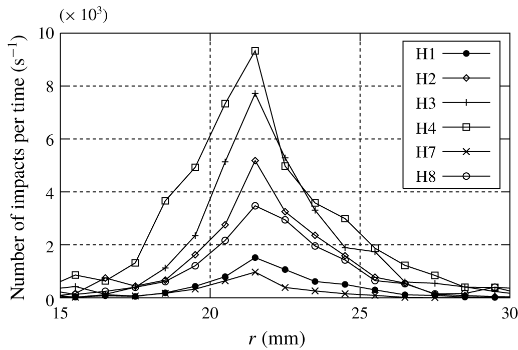
Figure 31. Number of collapses for different simulated cases versus radial distance from the nozzle’s central axis.
For collapses of  $\unicode[STIX]{x1D6FE}\leqslant 3$, we calculated the erosion potential for Lagrangian bubbles, $c_{ero,L}$, (see (3.62)) using our hybrid method. Additionally, we calculated the erosion potential from an Euler–Euler simulation, $c_{ero,E}$, (see (3.49)) for the same case based on the microjet model. Summing the erosion potentials, $c_{ero}$, of all faces in each radial interval yielded the erosion as a function of the radial distance, $r$, from the nozzle’s central axis. Figure 32 plots, as functions of $r$, the erosion potential, $c_{ero,E}$, obtained from a pure Euler–Euler simulation (using the Eulerian erosion model), the erosion potential, $c_{ero,L}$, obtained from a simulation based on the multi-scale approach (using the Lagrangian erosion model), and the experimentally measured erosion depths of Franc & Riondet (Reference Franc and Riondet2006). Maximum values of potentials obtained from the multi-scale method and from the Euler–Euler simulation compared favourably to maximum values of measured erosion depths (Exp.); however, the overall distribution of erosion potential from our hybrid method was narrower and agreed more closely with measured erosion depths. For collapse distances of $\unicode[STIX]{x1D6FE}<1$, far lesser impacts occurred than for collapse distances of $1\leqslant \unicode[STIX]{x1D6FE}\leqslant 3$. Although only collapses of $\unicode[STIX]{x1D6FE}<1$ were able to exceed the yield strength of the stainless steel 316 L target plate of $\unicode[STIX]{x1D70E}_{y}=400~\text{MPa}$, i.e. the material Franc & Riondet (Reference Franc and Riondet2006) used in their experiments. We concluded that our calculated collapses close to the surface were most aggressive. This was in agreement with experimental investigations on near-wall cavitation bubble collapses of Vogel & Lauterborn (Reference Vogel and Lauterborn1988), Isselin, Alloncle & Autric (Reference Isselin, Alloncle and Autric1998), Philipp & Lauterborn (Reference Philipp and Lauterborn1998) and Dular et al. (Reference Dular, Požar, Zevnik and Petkovšek2019) who found that near-wall collapses are most aggressive and that, for bubble collapses occurring at distances of $\unicode[STIX]{x1D6FE}>2$, almost no erosion takes place.
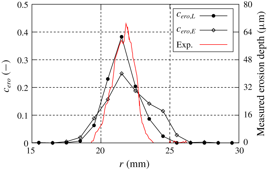
Figure 32. Numerical erosion assessment obtained from case H4 using our multi-scale method with a Lagrangian erosion model ( $c_{ero,L}$) and using an Eulerian erosion model ( $c_{ero,E}$) and comparative measured erosion depths of Franc & Riondet (Reference Franc and Riondet2006) (Exp.) plotted against radial distance from the nozzle’s central axis.
Recall that mass loss of material from an impacted surface depends nonlinearly on impact loads. We proposed that erosion is proportional to our calculated impact pressure squared (see (3.64)). Although most of our calculated impact pressures did not necessarily exceed the yield strength of  $\unicode[STIX]{x1D70E}_{y}=400~\text{MPa}$ for stainless steel 316 L, we assumed that all collapses within $\unicode[STIX]{x1D6FE}\leqslant 3$ impacted the surface of the target plate. To compare, we calculated the coefficient, $c_{ero,L2}$, by summing the coefficients from all other faces within radial intervals of 1 mm. Figure 33 plots, as functions of $r$, these coefficients, assuming a linear dependence, $c_{ero,L}$, and a nonlinear dependence of erosion on impact pressure, $c_{ero,L2}$, together with measured erosion depths of Franc & Riondet (Reference Franc and Riondet2006). Although the assumption of a quadratic proportionality in (3.64) was rough, our erosion assessment was improved and agreed more favourably with measured erosion depths, demonstrating that the nonlinear dependence of erosion on impact pressures is valid. Considering this nonlinear pressure dependence, the area of erosion was estimated to be narrower because not only most impacts, but also the impacts of highest pressures occurred at radial distances between 21 to 22 mm from the nozzle’s central axis.
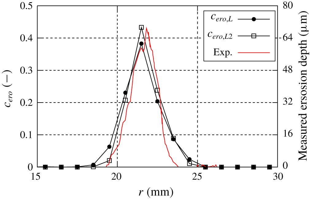
Figure 33. Numerical erosion assessment obtained from case H4 using our multi-scale method with a Lagrangian erosion model assuming a linear dependence ( $c_{ero,L}$) and assuming a nonlinear dependence on impact pressure ( $c_{ero,L2}$) and comparable measured erosion depths of Franc & Riondet (Reference Franc and Riondet2006) (Exp.) plotted against radial distance from the nozzle’s central axis.
6 Conclusion
We numerically simulated cavitating flow using a multi-scale Euler–Euler/Euler–Lagrange approach to assess cavitation erosion based on Lagrangian bubble collapses. The resulting simulated bubble dynamics was validated against experimental measurements, while bubble motions were verified for different cases. Our multi-scale approach treated large vapour volumes on an Eulerian grid; small vapour volumes, as spherical Lagrangian bubbles. To gain insight into bubble behaviour, the dynamics and motions of each Lagrangian bubble were solved individually. For one simple case and for the flow through an axisymmetric nozzle, the transformation mechanisms demonstrated the conversion of Eulerian vapour volumes into Lagrangian bubbles and vice versa. This multi-scale approach accounted for the interaction between macroscopic and microscopic scales involved in cavitating flows. To simulate the cavitating flow through an axisymmetric nozzle, we considered various characteristic parameters of the multi-scale solver and identified their influence on cavitation behaviour and erosion assessment. Although the average number of Lagrangian bubbles differed in all cases, these bubbles did not influence macroscopic cavitation. With the exception of a constant nucleus diameter of  $10~\unicode[STIX]{x03BC}\text{m}$, all our simulations showed a similar behaviour of macroscopic cavitation, and this behaviour compared favourably to cavitation obtained from a pure Euler–Euler simulation. Shedding frequencies obtained from pure Euler–Euler simulations agreed favourably with those obtained by Mihatsch et al. (Reference Mihatsch, Schmidt, Thalhamer, Adams, Skoda and Iben2011, Reference Mihatsch, Schmidt and Adams2015) who used a compressible solver to investigate the flow through this axisymmetric nozzle. As the distribution of cavitation nuclei can strongly influence cavitation behaviour, we additionally made use of a measurement-based distribution of nuclei based on experiments of Reuter et al. (Reference Reuter, Lesnik, Ayaz-Bustami, Brenner and Mettin2018). We assumed that this measurement-based nucleus distribution was reasonable because it provided the gas content of Lagrangian bubbles without considering additional assumptions.
To assess cavitation-induced erosion, we used information from calculated spherical Lagrangian bubble collapses and modelled the physics involved in an asymmetric near-wall bubble collapse based on well-recognised fundamental experiments and theoretical considerations. Our developed model using Lagrangian bubble collapses to estimate cavitation erosion was based on experimental measurements of Vogel & Lauterborn (Reference Vogel and Lauterborn1988) and Supponen et al. (Reference Supponen, Obreschkow, Tinguely, Kobel, Dorsaz and Farhat2016). The influence of the asymmetric collapse on bubble motion and collapse pressure depended on the stand-off distance of bubbles from the solid surface. Applying this model to simulations using our multi-scale approach enabled us to assess erosion that compared favourably to measured erosion depths of Franc & Riondet (Reference Franc and Riondet2006). Our simulations demonstrated that bubbles collapsing within a normalised stand-off distance of less than unity generated the highest impact pressures and coincided best with measured erosion depths. We conclude that the calculated collapses near to the wall contributed most to erosion, which is in agreement with experimental investigations on near-wall bubble collapses of Vogel & Lauterborn (Reference Vogel and Lauterborn1988), Isselin et al. (Reference Isselin, Alloncle and Autric1998), Philipp & Lauterborn (Reference Philipp and Lauterborn1998) and Dular et al. (Reference Dular, Požar, Zevnik and Petkovšek2019). Despite case H7, where the maximum bubble radius was limited, for all other hybrid simulations maximum collapse radii agreed favourably with investigations of Franc & Riondet (Reference Franc and Riondet2006) and Chahine (Reference Chahine2014). Furthermore, for the numerical collapse based erosion assessment, we found that erosion in the form of pit depth depended nonlinearly on impact pressures, which agreed with the erosion model of Franc & Riondet (Reference Franc and Riondet2006). By considering single Lagrangian bubble collapses, the possibility to assess cavitation erosion was significantly improved.
The physics-based assessment of erosion based on calculated single bubble collapses represents our principal contribution documented in this paper, and the experiments of Franc & Riondet (Reference Franc and Riondet2006) provided a reliable basis to validate our numerical approach. We established a connection between the behaviour of macroscopic cavitation structures and near-wall bubble collapses that cause erosion.
This approach offers the potential to correlate measured pits with bubble sizes. In future, hopefully additional data of single different sized bubble collapses, stand-off distances, pressure differences, and material properties will be made available from laser-induced bubble collapses near solid surfaces. Our approach made it possible to specify input data for simulations of isolated asymmetric bubble collapses. Plans call for applying our multi-scale approach to assess erosion sensitive regions for more complex flow problems, such as ship propellers.
Acknowledgements
This work was supported by the German Research Foundation (DFG grant EL 611/2-1). We acknowledge fruitful discussions of this work with U. Lantermann and F. Reuter. Furthermore, we gratefully acknowledge the computing time granted by the Center for Computational Sciences and Simulation (CCSS) of the University of Duisburg-Essen and provided on the supercomputer magnitUDE (DFG grants INST 20867/209-1 FUGG, INST 20876/243-1 FUGG) at the Zentrum für Informations- und Mediendienste (ZIM).
Declaration of interests
The authors report no conflict of interest.
Supplementary movies
Supplementary movies are available at https://doi.org/10.1017/jfm.2020.273.


 Open access