4.1. Surface elevation

Here we investigate the evolution of Gaussian-shaped broad-banded wave trains (2.14) by using the standalone FNP model and the hybrid FNP–NS model. We selected a series of representative wave trains with steepnesses of $k_0 \zeta _0=0.2$, $0.3$, $0.4$, $0.6$, $0.8$ and $1$. Computed surface elevations recorded at $x = 4.5$, $x = x_f =8.5\,\text {m}$ ($x_f$ is the expected focal point) and $x = 12.5\,\text {m}$ are plotted in figure 6. For wave trains with low steepness $k_0 \zeta _0 \leq 0.4$, there is only one mild breaking event or even no breaking at all. Thus the eddy viscosity closure was not used for the cases illustrated in (a–c).

Figure 6. Surface elevation variation with time obtained by three numerical models: VOF, BEMr and BEM$\nu$. The value of time in the horizontal axes was displaced using the group velocity $c_{g0}$ calculated for the carrier (peak) frequency of the wave train spectrum. The linear dispersive focusing is expected at $t-x/c_{g0} = 0$.

Figure 6(a) shows perfect coincidence of the results obtained by BEMr and VOF simulations when no breaking is present. It confirms the effectiveness of the BEM–VOF coupling used in the current study. The shape of the wave train at the focal point $x_f = 8.5\,\text {m}$ is very close to the linear prediction shown in figure 3(a). However, since the wave train is substantially nonlinear, a certain amount of asymmetry of the surface elevation before and after the focal point can be noticed. An increase in steepness, i.e. figures 6(b) and 6(c), leads to a significant deviation of either the BEMr solution or the VOF result from the linear estimation at the focal point, as expected for the steeper nonlinear waves. For the cases with higher steepness parameter $k_0 \zeta _0 \geq 0.6$ shown in figure 6(d–f), both the BEMr and BEM$\nu$ models were used. In compliance with the previous results, see § 3, no significant difference was noticed between the BEMr and BEM$\nu$ results. Therefore, further analysis in the paper will be based on the BEM$\nu$ model.

For wave trains with strong breaking shown in figure 6(d–f), the BEM$\nu$ and VOF models produced quite similar results at $x = 4.5\,\text {m}$. On the contrary, in the vicinity of and beyond the focal point, a considerable deviation between BEM$\nu$ and VOF results is found and it increases with the steepness $k_0 \zeta _0$. This indicates that certain physical processes associated with the breaking events are not accurately reflected by the quasi-potential eddy viscosity approximation in BEM$\nu$. It seems that this phenomenon is similar to the discrepancy we observed in § 3 for the experiments of Tian et al. (Reference Tian, Perlin and Choi2012) and Seiffert & Ducrozet (Reference Seiffert and Ducrozet2018).

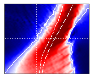
Flooding contours of the velocity magnitude underneath the free surface are plotted in figure 7 so that we can have a close look at the flow field to study the difference between the two-phase VOF solutions and the fully nonlinear potential BEM$\nu$ results. The fields are derived at $t = 35\,\text {s}$ near $x_f = 8.5\,\text {m}$ corresponding to the temporal and spatial location of the expected focal point according to the linear wave dispersion. The BEM$\nu$ model shows a quite smooth distribution of the velocity in the domain, contrary to the VOF solution, which embraces a certain perturbation component due to the vortical part of the flow. The plots show that the amplitude of the vortical velocity $-\boldsymbol {\nabla } \times \boldsymbol {\varPsi }$ is no longer small as assumed in the weakly damped theory used by Tian et al. (Reference Tian, Perlin and Choi2010, Reference Tian, Perlin and Choi2012). Consequently, the applicability of the eddy viscosity model for these problems is in question.

Figure 7. Distribution of the velocity magnitude $|\boldsymbol {U}|$ beneath the free surface obtained in the BEM$\nu$ and VOF models for three strongly breaking cases: (a) $k_0 \zeta _0 = 0.6$, (b) $k_0 \zeta _0 = 0.8$ and (c) $k_0 \zeta _0 = 1.0$. The plots are obtained at the instant of focusing $t_f = 35\,\text {s}$ and in the vicinity of the focal point $x_f = 8.5\,\text {m}$: the horizontal scale is $8 \leq x \leq 10.5\,\text {m}$.

It is expected that the vortical flow consists of sheared currents and other local and distributed non-potential fluid motions (Iafrati et al. Reference Iafrati, Babanin and Onorato2013; Deike et al. Reference Deike, Pizzo and Melville2017; Lenain et al. Reference Lenain, Pizzo and Melville2019). For instance, several vortical structures are clearly shown in figures 7(b) and 7(c). A more detailed investigation of the non-potential flows supposes the need of quantitative comparison of the BEM$\nu$ and VOF velocity fields. However, a meaningful comparison is practically impossible for the considered cases because the shapes of free surface obtained by these models are very different.

4.2. Energy dissipation due to wave breaking

The spatio-temporal evolution of the wave train calculated by the BEM$\nu$ model is illustrated in figure 8 in terms of surface elevation. Wave breaking regions are highlighted in the figure as rectangular areas enclosed by black solid lines. The dimensions of these regions $L_b$ in space and $T_b$ in time were determined by the eddy viscosity closure (2.6). For each region the constant value of the eddy viscosity $\nu _{{eddy}}$ was calculated by using the formula (2.5). As expected, the non-breaking case, i.e. figure 8(a), does not have any predicted breaking locations. We also note that increasing the steepness $k_0 \zeta _0$ can cause multiple breaking events instead of a single very strong one. This is because the wave train loses its stability much ahead of the focal point. At the same time, larger values of $\nu _{{eddy}}$ correspond to more energy dissipation.

Figure 8. Energy dissipation regions predicted by the eddy viscosity approximation. (a–f) Present the wave trains having steepness parameter $k_0 \zeta _0 = 0.2,\ 0.3,\ 0.4,\ 0.6,\ 0.8,\ \text {and}\ 1.0$, respectively. The breaking regions are depicted by black solid lines. Colour shows the spatio-temporal variation of the surface elevation $\eta (x,t)$ calculated by the BEM$\nu$ model. Dashed lines show the location of the focal point expected according to the linear dispersion.

The energy dissipation locations shown in figure 8 do not overlap with each other. This means that in the studied wave trains, waves always break at different locations. Before the focal point, breaking always appears at the leading edge of the wave train because of the presence of short steep waves. On the contrary, after the focal point breaking locations move closer to the centre of wave train. Taking into account the fact that the leading edge of the wave train after the focal point consists of long waves, it can be assumed that those waves are more stable. This observation is usually involved in the spectral models of water waves, where the energy dissipation mostly at high frequencies is incorporated (Babanin et al. Reference Babanin, Waseda, Kinoshita and Toffoli2011; Annenkov & Shrira Reference Annenkov and Shrira2018).

Within the eddy viscosity quasi-potential approach, the energy dissipation process can probably be seen as a transformation of the energy associated with surface gravity waves into the rotational fluid flow energy. Since the considered broad-banded wave train occupies a restricted space, it is convenient to estimate the strength of wave breaking by tracing the amount of energy transferred by the wave train through different cross-sections, i.e. integral energy flux (Banner & Peirson Reference Banner and Peirson2007; Drazen, Melville & Lenain Reference Drazen, Melville and Lenain2008; Tian, Perlin & Choi Reference Tian, Perlin and Choi2008; Derakhti & Kirby Reference Derakhti and Kirby2016). Taking into account that wave breaking is a strongly localised phenomenon, energy loss is associated with a particular location and appears as a reduction of the integral energy flux across the breaking location.

The total integral energy flux passing through the cross-section $x$ in the VOF model is given by

(4.1)\begin{equation} F_{VOF}^{NL}(x) = \int_{-\infty}^{+\infty} \textrm{d} t \int_{{-}h}^{\eta(x,t)} \left\lbrace \frac{1}{2} \rho_w \left| \boldsymbol{U} \right|^2 + \rho_w g z + p\right\rbrace u \beta \,\textrm{d} z,\end{equation}

where $\boldsymbol {U} = (u, w)$. This expression does not involve any physical simplification and thus determines the fully nonlinear value of the energy flux. In the VOF model, the volume fraction $\beta$ is used to determine the percentage of water contained in a mesh cell. Thus the height of the water layer in each cell is $\beta dz$. The so-called dry and wet cells are distinguished by $\beta =0$ and $\beta = 1$, respectively. Determination of the nonlinear energy flux in the BEM$\nu$ model is more complicated because the needed pressure $p$ is not readily available in the solution. Simplification of (4.1) can be achieved by using the Bernoulli equation (2.3) and taking $\boldsymbol {U} = -\boldsymbol {\nabla } \varphi$

(4.2)\begin{equation} F_{BEM}^{NL}(x) ={-} \rho_w \int_{-\infty}^{+\infty} \textrm{d} t \int_{{-}h}^{\eta(x,t)}\frac{\partial \varphi}{\partial t} \frac{\partial \varphi}{\partial x} \textrm{d} z .\end{equation}

In laboratory it is not feasible yet to measure the nonlinear energy flux. Instead, a linearisation of (4.2) is usually applied (Banner & Peirson Reference Banner and Peirson2007; Drazen et al. Reference Drazen, Melville and Lenain2008; Tian et al. Reference Tian, Perlin and Choi2008, Reference Tian, Perlin and Choi2010, Reference Tian, Perlin and Choi2012; Derakhti & Kirby Reference Derakhti and Kirby2016; Seiffert & Ducrozet Reference Seiffert and Ducrozet2018). Researchers usually assume the equipartition of total energy between the kinetic and potential parts, which is admissible for linear wave system. The linear approximation for the total energy density is $E = \rho _w g \overline {\eta ^2}$, where the overbar represents averaging over the local wavelength. The linear approximation for the energy flux is then given by (Dean & Dalrymple Reference Dean and Dalrymple1991; Drazen et al. Reference Drazen, Melville and Lenain2008; Derakhti & Kirby Reference Derakhti and Kirby2016)

(4.3)\begin{equation} F^{L}(x) = \int_{-\infty}^{+\infty} E c_{gs}\,\textrm{d} t = \int_{-\infty}^{+\infty} \rho_w g c_{gs} \eta^2 \,\textrm{d} t .\end{equation}

Here, $c_{gs}$ is the spectral-weighted group speed approximating the velocity of energy transferred by the given wave train

(4.4)\begin{equation} c_{gs} = \frac{\sum_j c_{g,j} a_j^2}{\sum_j a_j^2}, \end{equation}

where $a_j$ and $c_{g,j}$ are the amplitude and the group velocity of the $j$th component of the wave packet spectrum.

The outcomes of (4.1) and (4.3) are compared in figure 9(a) for the steepest wave train with $k_0 \zeta _0 = 1.0$. The dimensionless variables are introduced: energy flux $\hat {F} = F / F_0$ and spatial coordinate $\hat {x} = x / \lambda _0$; $F_0$ is the initial energy flux computed at $x \approx 0$. Figure 9(a) shows that the distributions of linear energy flux computed by the BEM$\nu$ and VOF models, i.e. $F_{{BEM}\nu }^L$ and $F_{{VOF}}^L$, somewhat deviate from each other. The nonlinear energy flux $F_{{VOF}}^{NL}$ obtained by the VOF model provides the highest values of $\hat {F}$. In spite of the different trajectories of $F_{{BEM}\nu }^L$ and $F_{{VOF}}^{NL}$, the bulk amount of energy dissipation computed by the VOF and BEM$\nu$ models are close to each other for the cases considered here as shown in figure 9(b). This suggests that the eddy viscosity approximation used in the BEM$\nu$ model predicts quite accurately the energy dissipation process, in agreement with earlier investigations (Tian et al. Reference Tian, Perlin and Choi2010, Reference Tian, Perlin and Choi2012; Seiffert & Ducrozet Reference Seiffert and Ducrozet2018; Hasan et al. Reference Hasan, Sriram and Selvam2019). It is interesting to note that the discrepancy in surface elevation calculation (see figure 6) does not significantly affect the amount of wave energy dissipated by breaking.

Figure 9. (a) Distribution of the dimensionless integral energy flux $\hat {F} = F / F_0$ along the computational domain $\hat {x} = x / \lambda _0$ for the wave train with the steepness parameter $k_0 \zeta _0 = 1$. Black dashed line corresponds to the best fit of the nonlinear energy flux $F_{{VOF}}^{NL}$. (b) Dimensional integral energy flux computed for the wave trains of different steepness. Solid lines: VOF simulations ($F_{{VOF}}^{NL}$); dashed lines: BEM$\nu$ simulations ($F_{{BEM}\nu }^{L}$).

In the present work, we use the mean gradient of nonlinear energy flux $\hat {F}_{\hat {x}} = - \textrm {d} \hat {F} / \textrm {d} \hat {x}$ to characterise the strength of breaking. Such a quantify can be interpreted as the wave energy dissipation rate in space. For the VOF model, we produced the best fit of the energy flux $F_{{VOF}}^{fit}$ and illustrated it in figure 9(a) as the black dashed line, which has a gradient of 0.0313 in magnitude. The distributions of $F_{{VOF}}^{NL}$ and $F_{{VOF}}^{fit}$ for wave trains with different steepness $k_0 \zeta _0$ are plotted in figure 10. The calculated values of $\hat {F}_{\hat {x}}$ are summarised in table 4. It can be seen from figure 10 and table 4 that the energy dissipation rate $\hat {F}_{\hat {x}}$ increases with the wave train steepness $k_0 \zeta _0$.

Figure 10. Distribution of the nonlinear energy flux $F_{{VOF}}^{NL}$ obtained by the VOF model. The solid curves correspond to energy fluxes produced by the wave trains of different steepness $k_0 \zeta _0$. The dash-dotted lines show the best fit of the data needed to compute the energy dissipation rate $\hat {F}_{\hat {x}}$.

Table 4. The values of the energy dissipation rate and the equivalent depth-uniform current computed for the wave trains of different steepness.

Based on a scaling analysis, the breaking parameter $b$ was used by Duncan (Reference Duncan1983) and Drazen et al. (Reference Drazen, Melville and Lenain2008) to characterise energy dissipation caused by wave breaking. This parameter provides a quantitative relationship between the kinematics of breaking and the dynamics of energy loss. Importantly, the value of this parameter can be estimated from the field observations of whitecaps (Drazen et al. Reference Drazen, Melville and Lenain2008). It can be instructive to quantify the value of the parameter $b$ for the computations performed in the current study. This will also allow us to assess the genuineness of numerical models by comparing the calculated results against a set of published experimental and computational data.

According to Derakhti & Kirby (Reference Derakhti and Kirby2016) the parameter $b$ can be introduced by involving numerical results in the following way:

(4.5)\begin{equation} b \rho_w g^{{-}1} c_b^5 = \epsilon = \frac{\int_{x,t} {\rm \Delta} F}{\tau_b}, \end{equation}

where $\epsilon$ is the averaged wave energy dissipation rate, $\rho _w$ is the water density, $c_b$ is the phase speed of the breaking crest, ${\rm \Delta} F$ is the loss of the total wave energy flux according to (4.1) or (4.3). The time scale of active breaking is related to the period of breaking wave as $\tau _b = \alpha _t T_b$. According to Drazen et al. (Reference Drazen, Melville and Lenain2008), Kleiss & Melville (Reference Kleiss and Melville2010), and Derakhti & Kirby (Reference Derakhti and Kirby2016), here, the proportionality constant is taken as $\alpha _t = 0.75$. The wavenumber $k_b$ of a breaking wave is determined from the geometry of the breaking crest according to Tian et al. (Reference Tian, Perlin and Choi2010, Reference Tian, Perlin and Choi2012) and Derakhti & Kirby (Reference Derakhti and Kirby2016). Other parameters for the breaking crest are related to $k_b$ as follows: $c_b = (g / k_b \,\text {tanh}\, k_b h)^{1/2}$; $T_b = 2 {\rm \pi}/ (k_b c_b)$. After substituting these into (4.5) we can obtain

(4.6)\begin{equation} b = \frac{g \int_{x,t} {\rm \Delta} F}{\alpha_t \rho_w \overline{c_b}^5 \overline{T_b}}. \end{equation}

Since multiple breaking events are observed in our simulations, the averaged parameters of the breaking crest are used as shown in the expression (4.6). Note that the total energy flux losses obtained by the VOF and BEM$\nu$ models are very close to each other as shown in figure 9(b).

The calculated values of breaking parameter $b$ (4.6) are compared with previously published results in figure 11(a). The widely used empirical parametrisation for $b$ as a function of linear wave slope $S$ is adopted from Romero, Melville & Kleiss (Reference Romero, Melville and Kleiss2012): ${b = 0.4 (S - 0.08)^{5/2}}$. The wave slope $S$ is the maximal wave steepness calculated for the linearly evolving wave train. For our cases one can estimate it as ${S = k_0 \zeta _0}$ (see figure 4). It is clearly illustrated in figure 11 that the values of $b$ calculated in our study by both VOF and BEM$\nu$ models compare well with the empirical expression of Romero et al. (Reference Romero, Melville and Kleiss2012) and experimental data reported in the literature. Moreover, we present the result for a highly energetic breaking event under the condition $S > 0.8$, which has not yet been reported in the literature to the best of our knowledge. It is interesting to note that even for such strong wave energy dissipation, the parametrisation of Romero et al. (Reference Romero, Melville and Kleiss2012) is still applicable. Figure 11(b) suggests an exponential dependence of the breaking parameter $b$ on the energy dissipation rate $\hat {F}_{\hat {x}}$. For the wave trains considered in the present study the following empirical expression can be suggested: $b = 3 \times 10^{-3} \exp (1.5 \times 10^2 \times \hat {F}_{\hat {x}})$.

Figure 11. (a) Breaking parameter $b$ as a function of the maximum wave steepness in the course of the linear wave train evolution, i.e. $S = k_0 \zeta _0$, see figure 4. Solid line: empirical expression based on scaling argument from Romero et al. (Reference Romero, Melville and Kleiss2012). The present simulations are in agreement with experimental and other reported numerical studies. The reference data are from the works of Melville (Reference Melville1994), Banner & Peirson (Reference Banner and Peirson2007), Drazen et al. (Reference Drazen, Melville and Lenain2008), Derakhti & Kirby (Reference Derakhti and Kirby2016) and Deike, Popinet & Melville (Reference Deike, Popinet and Melville2015); Deike, Melville & Popinet (Reference Deike, Melville and Popinet2016); Deike et al. (Reference Deike, Pizzo and Melville2017). (b) Breaking parameter $b$ as a function of the energy dissipation rate $\hat {F}_{\hat {x}}$, see table 4.

4.3. Shift of phase due to wave breaking

In the beginning and at the end of computations only a part of the wave train is present within the domain. Therefore, in the analysis we focus on the interval ${30 \leq t / T_0 \leq 56.8}$, when the full length of the wave train is present within the domain. The surface elevation of free waves (2.19) obtained by the spectral decomposition (see § 2.5) of simulation results can be written as

(4.7)\begin{equation} \eta^{(1)}(x) = \sum_{m=0}^M\left| A(k_m) \right| \cos(k_m x + \xi_m), \end{equation}

where the phase is given by

(4.8)\begin{equation} \xi_m = \tan^{{-}1} \frac{\textrm{Im}\{ A(k_m) \} }{\textrm{Re}\{ A(k_m) \} }. \end{equation}

It was found that the amplitude spectra obtained from the BEM$\nu$ and VOF simulations are practically identical in terms of the absolute value of the amplitude $|A(k_m,\omega _m)|$ regardless of wavenumber and angular frequency, cf. figure 12(a–d). This observation confirms the capability of the eddy viscosity approximation in predicting wave energy dissipation, which is in line with previous studies (Tian et al. Reference Tian, Perlin and Choi2010, Reference Tian, Perlin and Choi2012; Seiffert & Ducrozet Reference Seiffert and Ducrozet2018; Hasan et al. Reference Hasan, Sriram and Selvam2019), see also figure 9. Note that the energy contained in the spectrum is $\sum _{m=0}^M |A(k_m,\omega _m)|^2$. Therefore the visible divergence in surface elevation shown in figure 6 is very likely caused by the phase $\xi _m$. The phase difference between the VOF and BEM$\nu$ results relative to the carrier wave characteristics $\omega _0 T_0$ is given by

(4.9)\begin{equation} \frac{{\rm \Delta} \xi_m}{\omega_0 T_0} =\frac{1}{2 {\rm \pi}} \left(\xi_{m,{VOF}} - \xi_{m,{BEM}\nu} \right) .\end{equation}

The evolution of ${\rm \Delta} \xi _m$ in time for different wavenumber $k_m$ is plotted in figure 13 for the wave trains with steepness $k_0 \zeta _0 \geq 0.4$.

Figure 12. Free wave spectra obtained in VOF (solid lines) and BEM$\nu$ (dashed lines) models. (a–d) Present the wave trains of different steepness parameter $k_0 \zeta _0$. Plots of different colour are obtained at various times of simulations.

Figure 13. Evolution of difference in the free waves phases ${\rm \Delta} \xi _m$ between VOF and BEM$\nu$ simulations. The colour scheme from blue to red displays the plots obtained at different instances within the range $30 \leq t / T_0 \leq 56.8$. Grey plots show other not coloured data within the same time interval. (a–d) Correspond to the wave trains of various steepness $k_0 \zeta _0$.

Figure 13 reveals a quite smooth and deterministic rather than stochastic evolution of the phase shift ${\rm \Delta} \xi$ in time. Moreover, there is a strong dependence of ${\rm \Delta} \xi$ on the wavenumber. The phase shift is relatively small at low wavenumbers, while at a high wavenumber it has a much pronounced growth with time. For instance, at the end of the wave breaking region the phase shift for a high wavenumber $k/k_0 \approx 1.5$ can increase by more than one full revolution, see figure 13(d). If the wave train steepness $k_0 \zeta _0$ and subsequently the energy dissipation rate $\hat {F}_{\hat {x}}$ are relatively low, the corresponding phase shift is much weaker, see figure 13(a). The phase difference between the BEM$\nu$ and VOF calculations could be due to the fact that the highly nonlinear rotational flows generated by breaking cannot be properly handled by the weakly potential eddy viscosity approximation.

Considering the dependence of phase shift on the wavenumber $k$ and time $t$ for the breaking strength $\hat {F}_{\hat {x}}$, we approximate it with the following expression:

(4.10)\begin{equation} \left.\frac{{\rm \Delta} \xi}{\omega_0 T_0}\right|_{\hat{F}_{\hat{x}}} = \varXi \left[ \frac{k}{k_0} \right]^{\varTheta_K}\left[ \frac{t}{T_0} \right]^{\varTheta_T}. \end{equation}

The values of three coefficients $\varXi$, $\varTheta _K$ and $\varTheta _T$ change from one wave train to another due to different breaking strength. We applied the least squares method to obtain the dependencies $\varXi (\hat {F}_{\hat {x}})$, $\varTheta _K (\hat {F}_{\hat {x}})$ and $\varTheta _T (\hat {F}_{\hat {x}})$ from the numerical simulations, and present them in figure 14. It is shown that the rate of phase shift has a nonlinear dependence on time and wavenumber for relatively weak breaking; i.e. the values of the power coefficients $\varTheta _K \approx \varTheta _T \approx 4$ when $\hat {F}_{\hat {x}} < 0.01$. If breaking is strong, the dependence of phase shift on time tends to be linear with $\varTheta _T \approx 1$, while the dependence on wavenumber is close to quadratic with $\varTheta _K \approx 2$. Both $\varTheta _K$ and $\varTheta _T$ are reduced almost linearly with the increase of breaking strength $\hat {F}_{\hat {x}}$. In turn, the proportionality coefficient $\varXi (\hat {F}_{\hat {x}})$ demonstrates an exponential dependence on the energy dissipation rate $\hat {F}_{\hat {x}}$. Therefore it seems reasonable to infer from the analysis that the phase shift can become quite significant for strong-breaking events.

Figure 14. Dependence of the fitting coefficients $\varXi$, $\varTheta _K$ and $\varTheta _T$ (4.10) on the wave breaking strength $\hat {F}_{\hat {x}}$.

We applied the similar interpolation function to all the considered wave trains and obtained the corresponding phase shift in a dimensionless form

(4.11)\begin{equation} \frac{{\rm \Delta} \xi}{\omega_0 T_0} =\varXi \left[ \hat{F}_{\hat{x}} \right]^{\varTheta_F} \left[ \frac{k}{k_0} \right]^{\varTheta_K}\left[ \frac{t}{T_0} \right]^{\varTheta_T}. \end{equation}

Applying the least squares fitting of the numerical results, we obtained the coefficients and listed them in table 5. In addition to the previous findings, the value of $\varTheta _F \approx 2$ implies a quadratic dependence of the phase shift on the energy dissipation rate.

Table 5. Values of the dimensionless coefficients in the expression (4.11).

In figure 15 the raw plots of ${\rm \Delta} \xi (k, t)$ obtained from the numerical simulations are compared with those reconstructed from (4.11) in order to study the accuracy of the suggested approximation. It can be noticed that the plots obtained directly from the simulations using (4.9), see (a,c), exhibit fluctuations at high wavenumbers because the bound waves are not perfectly separated from the free waves by the decomposition method (§ 2.5). Even minor presence of unseparated bound waves significantly influences the phases of harmonics. Function (4.11) filters the fluctuations from the plots as presented in (b,d), while keeping a good qualitative and quantitative correspondence with the raw data extracted from the simulations.

Figure 15. Phase shift ${\rm \Delta} \xi / \omega _0 T_0$ as a function of wavenumber and time obtained for the wave trains of different breaking strength: (a,b) $\hat {F}_{\hat {x}} = 0.0196$; (c,d) $\hat {F}_{\hat {x}} = 0.0313$. (a,c) Present the raw phase shift calculated using (4.9), while (b,d) are plotted using the interpolation (4.11).

The observed shift in phase is possibly related to the so-called phase-locking phenomenon reported by Derakhti & Kirby (Reference Derakhti and Kirby2016). The phase-locking process is considered as a nonlinear linkage between high- and low-frequency wave components. This linkage was demonstrated by analysing the wavelet spectra of the surface elevation in the vicinity of the breaking event (Derakhti & Kirby Reference Derakhti and Kirby2016). The propagation velocity of the high frequency components of the breaking wave was found to be different from that of the pre-breaking but stable wave.

4.4. Dispersion variation

It has been shown in various studies that the relationship between wavenumber and frequency may deviate from the linear dispersion relation (2.13) when the frequency spectrum is narrow. Krogstad & Trulsen (Reference Krogstad and Trulsen2010) studied the dynamic nonlinear evolution of unidirectional Gaussian wave packets using the nonlinear Schrödinger equation and its generalisations. It was observed that in the $k$–$\omega$ space the spectrum does not maintain a thin well-defined dispersion surface but develops into continuous distribution. The spectral components above and below the spectral peak were found to have the phase and group velocities close to that of the spectral peak. It was concluded that in some cases it is inappropriate to use the linear dispersion relation for the post-processing of experimental data.

Houtani et al. (Reference Houtani, Waseda, Fujimoto, Kiyomatsu and Tanizawa2018a) and Houtani, Waseda & Tanizawa (Reference Houtani, Waseda and Tanizawa2018b) have demonstrated that the dispersion characteristics of the Akhmediev breather solution to the nonlinear Schrödinger equation in deep water deviates significantly from the linear relationship (2.13). It was also shown that these findings extend beyond the applicability of nonlinear Schrödinger equation. Accordingly, the highly nonlinear non-breaking modulated wave trains also maintain the straight line relationship between the wavenumber and the instantaneous frequency; this line is tangent to the dispersion relation curve (2.13) at the carrier wavenumber. Gibson & Swan (Reference Gibson and Swan2006) investigated the waves dispersion using the numerical simulations based on the third-order Zakharov equation. Inconsistency of the simulation results with the linear wave dispersion (2.13) was explained by analysing the third-order resonant interactions. The nonlinear energy transfer between harmonics in the free wave spectrum alters the values of the complex amplitudes. If interacting wave components are out of phase, this energy transfer will change the instantaneous phases of waves, which is reflected in the $k$–$\omega$ space. Adopting a similar Zakharov equation based theoretical model, the nonlinear correction to the dispersion relation for gravity waves in a constant depth was derived analytically by Stuhlmeier & Stiassnie (Reference Stuhlmeier and Stiassnie2019).

The phase of each free wave component is (Houtani et al. Reference Houtani, Waseda, Fujimoto, Kiyomatsu and Tanizawa2018a,Reference Houtani, Waseda and Tanizawab)

(4.12)\begin{equation} \xi (k, \omega, t) = k x - \omega t - \delta^{NL} (k, t),\end{equation}

where $\delta ^{NL} (k, t)$ is the slowly varying nonlinear phase induced by the third-order resonant interaction between the waves (Gibson & Swan Reference Gibson and Swan2006). The angular frequency can be found from (4.12) by involving (2.13)

(4.13)\begin{equation} \omega (k) ={-} \frac{\partial \xi(k, \omega, t)}{\partial t} = \sqrt{g k \tanh (k h)}+ \left\langle \frac{\partial \delta^{NL}(k, t)}{\partial t} \right\rangle. \end{equation}

When analysing a long time evolution of the wave group, the influence of $\left \langle \partial \delta ^{NL} / \partial t \right \rangle \neq 0$ seen in $k$–$\omega$ spectrum may be interpreted as a deviation of the relationship $\omega (k)$ from (2.13).

In the current study it was found that the nonlinear contribution $\delta ^{NL}(k, t)$ can be caused by the resonant interactions as well as the breaking-induced rotational flows. To construct the $k$–$\omega$ spectrum from BEM$\nu$ and VOF computations the discrete distribution of the surface elevation in space is extracted from the numerical results. After applying spectrum decomposition (see § 2.5) the elevations of free waves at different instants are expressed as a function $\eta (x,t)$. The discrete 2-D Fourier transform of this function in the $k$–$\omega$ space is given by

(4.14)\begin{equation} \hat{\eta} (k, \omega) = \frac{1}{N M} \sum_{x} \sum_{t} \eta (x, t) \exp({\textrm{i} (k x - \omega t)}),\end{equation}

where $N$ and $M$ are the number of discrete values of $\eta$ in $x$ and $t$ directions, respectively. Distributions of the absolute values $|\hat {\eta } (k, \omega )|$ obtained from the VOF simulations are shown in figure 16.

Figure 16. Dimensionless free wave $k$–$\omega$ spectrum $|\hat {\eta } (k, \omega )| / \max (|\hat {\eta } (k, \omega )|)$ obtained from the VOF simulations for wave packets with different steepness. A logarithmic colour scale is used. Solid line represents the linear dispersion curve (2.13) with capillary effects accounted for; dashed and dash-dotted lines show dispersion curves obtained by weighting (4.15) applied to BEM$\nu$ and VOF computation results, respectively.

The highest values of $|\hat {\eta } (k, \omega )|$ are located in a relatively narrow region approximately defining the dispersion relation $\omega (k)$. For the considered broad-banded Gaussian wave trains the distributions of $|\hat {\eta } (k, \omega )|$ have no visible deviation from the linear dispersion relation for both non-breaking and weakly breaking cases $k_0 \zeta _0 = 0.3\text {--}0.4$, cf. figures 16(a) and 16(b). According to figure 4, the maximum steepness of these wave trains is within the interval ${0.2 < \varepsilon _{max} < 0.4}$, indicating strong nonlinearity. Such dispersive properties are different from those discussed in Gibson & Swan (Reference Gibson and Swan2006), Krogstad & Trulsen (Reference Krogstad and Trulsen2010) and Houtani et al. (Reference Houtani, Waseda, Fujimoto, Kiyomatsu and Tanizawa2018a,Reference Houtani, Waseda and Tanizawab), where the linear dispersion relation was found to be inaccurate. The difference in the wave packet evolution may be related to: (i) the width of the spectra that is significantly higher for the wave trains considered in the current study, and (ii) the reduction of wave steepness and nonlinear effects away from the focusing location.

Subsequent increase of the wave train steepness, i.e. $k_0 \zeta _0 > 0.4$, accompanied by the intensification of wave breaking leads to the deviation of the distribution of $|\hat {\eta } (k, \omega )|$ from the linear dispersion curve (2.13), cf. figure 16(c–e). The magnitude of this deviation is dependent on the wave train steepness parameter $k_0 \zeta _0$. Note that the wave trains with ${k_0 \zeta _0 \geq 0.6}$ are subject to breaking within the entire range of $t$ and $x$ used for computing the $k$–$\omega$ spectrum. Moreover, the deviation is observed only for the wavenumbers above the spectral peak $k_0$, while long waves always follow the linear dispersion. To some extent, this phenomenon is correlated to the phase shift plotted in figures 13 and 15, which is also present at high wavenumbers only.

The dependency of frequency on wavenumber $\omega (k)$ can be approximated from the distribution of $|\hat {\eta } (k, \omega )|$ by using the following weighting:

(4.15)\begin{equation} \omega (k_n) = \frac{\sum_m \omega_m |\hat{\eta} (k_n, \omega_m)|^2} {\sum_m |\hat{\eta} (k_n, \omega_m)|^2}.\end{equation}

The outcomes of applying such a weighting to the BEM$\nu$ and VOF simulations are plotted in figure 16(c–e) by dashed and dash-dotted lines. It is interesting to note that the dispersion curves of BEM$\nu$ and VOF are quite close to each other in (c), and both deviate from the linear dispersion curve. A further increase in breaking intensity, see (d,e), leads to a pronounced deviation of the VOF curve from the BEM$\nu$ one. This suggests that the nonlinearities in the potential wave fields are only partially responsible for the change of dispersion.

Approximate dispersion relations obtained from the BEM$\nu$ and VOF results based on (4.15) are plotted in figure 17(a) for the steepest wave packet $k_0 \zeta _0 = 1.0$. It can be noticed that the weakly nonlinear dispersion relation (Melville Reference Melville1983; Whitham Reference Whitham1999)

(4.16)\begin{equation} \frac{\omega^2}{g k \tanh k h} =1 + \left(\frac{9 \tanh^4 kh - 10 \tanh^2 k h + 9}{8 \tanh^4 k h} \right) \varepsilon^2\end{equation}

that takes into account the actual mean steepness of waves can largely explain the deviation of dispersion observed in the BEM$\nu$ model. In (4.16) we assume the steepness to be of the order $\varepsilon \sim 0.3$ since the considered wave packet is constantly subject to breaking. This suggests that the effects observed in the BEM$\nu$ model are probably caused by the nonlinear wave train evolution rather than the application of empirical eddy viscosity breaking approximation. See Appendix C for more discussion on this. To get further insights into the actual wave train dispersion observed in VOF computations, we attempt to correct the BEM$\nu$ dispersion curve by involving the estimate of phase shift (4.11) and the expression (4.13)

(4.17)\begin{equation} \omega(k) = \omega_{BEM\nu}(k) +\left\langle \frac{\partial {\rm \Delta} \xi}{\partial t} \right\rangle \approx\omega_{BEM\nu} \left\langle 1 + \varTheta_T \varXi \left[ \hat{F}_{\hat{x}} \right]^{\varTheta_F} \left[ \frac{k}{k_0} \right]^{\varTheta_K}\left[ \frac{t}{T_0} \right]^{\varTheta_T-1}\right\rangle. \end{equation}

Taking into account $(\varTheta _T-1) \sim 0$, the expression (4.17) can be simplified as

(4.18)\begin{equation} \omega(k) =\omega_{BEM\nu} \left(1 + \varTheta_T \varXi \left[ \hat{F}_{\hat{x}} \right]^{\varTheta_F} \left[ \frac{k}{k_0} \right]^{\varTheta_K}\right).\end{equation}

The corrected dispersion curve (4.18) for the BEM$\nu$ model plotted in figure 17(a) is close to the VOF model. This suggests that the difference in wave dispersion between the two models is caused by the phase shift phenomenon discussed in § 4.3.

Figure 17. Dependence of (a) angular frequency and (b) phase speed on the wavenumber obtained from the results of BEM$\nu$ and VOF simulations using (4.14) and (4.15). The correction to the BEM$\nu$ curve is obtained by using (4.18). The steepest wave train is considered: $k_0 \zeta _0 = 1.0$, $\hat {F}_{\hat {x}} = 0.03134$. The linear (2.13) and the weakly nonlinear (4.16) dispersion relations are given for reference.

A similar observation regarding the satisfactory accuracy of (4.16) for steep non-breaking wave trains has previously been reported in the experimental study of Melville (Reference Melville1983), in which local phases were extracted from the surface elevation measurements by using the Hilbert transform. Nevertheless, Stansell & MacFarlane (Reference Stansell and MacFarlane2002) questioned the physical significance of phase reversal effect emphasised by Melville (Reference Melville1983) (reduction of the local phase speed below zero), as it can be subject to the peculiarity of Hilbert transform. On the other hand, Banner et al. (Reference Banner, Barthelemy, Fedele, Allis, Benetazzo, Dias and Peirson2014), Fedele, Chandre & Farazmand (Reference Fedele, Chandre and Farazmand2016) and Fedele, Banner & Barthelemy (Reference Fedele, Banner and Barthelemy2020) showed that the crest speed of a nearly breaking wave can significantly deviate from the phase speed suggested by both (2.13) and (4.16). The actual wave crest speed exhibits very fast variations: whether a crest experiences slowing down or speeding up depends on the dispersion regime it belongs to. Theoretical analyses demonstrated that quite complicated linear and nonlinear processes can be involved in this phenomenon. Though the present study is not aimed at addressing the complicated kinematics of breaking wave crests, it is of interest to analyse the dependence of phase speed on the wavenumber $c_p(k) = \omega / k$ evaluated from the dispersion relationships, see figure 17(b). Linear and BEM$\nu$ dispersions show significant variation of the value of $c_p$ within the considered range of the wavenumbers. On the other hand, the VOF data suggest a constant value of $c_p$ at high wavenumbers. This implies that relatively short waves propagate at a similar speed. Note that capillarity in (2.13) has an insignificant effect within the considered range of wavenumbers. Contrary to the observations of Houtani et al. (Reference Houtani, Waseda, Fujimoto, Kiyomatsu and Tanizawa2018a,Reference Houtani, Waseda and Tanizawab), the property $c_p \neq c_p(k)$ is only held for high wavenumbers in the considered case.

Ramamonjiarisoa & Mollo-Christensen (Reference Ramamonjiarisoa and Mollo-Christensen1979) studied the dispersion anomalies of wind waves. They reported that the phase velocities for frequencies above the dominant wave are nearly constant and almost equivalent to the dominant wave's phase velocity. For mechanically generated narrow-banded wave trains, they noted the absence of such an effect except for a specific wave train subject to breaking. It is also found in their work that once the wave train starts to break, the harmonics above the carrier wave propagate at a very similar phase speed. Despite the experiments of Ramamonjiarisoa & Mollo-Christensen (Reference Ramamonjiarisoa and Mollo-Christensen1979) are based on narrow-banded wave trains, the observed effect they documented is possibly related to the phase shift phenomenon discussed in the current study. It is also important to note that Ramamonjiarisoa & Mollo-Christensen (Reference Ramamonjiarisoa and Mollo-Christensen1979) did not report/observe any deviation of the dispersion relation for nearly breaking wave trains. Therefore, rather than being induced by the nonlinearities of the potential wave field, the deviation of wave dispersion is more likely caused by the non-potential flows generated by wave breaking or wind.

We note that the expression (4.18) can be written in another form

(4.19)\begin{equation} \omega(k) =\omega_{BEM\nu} + k \times \tilde{U}. \end{equation}

Here, the empirical constant ${\tilde {U} = \varTheta _T \varXi \hat {F}_{\hat {x}}^{\varTheta _F} \overline {c_{BEM\nu }}}$ can probably be considered as the velocity of an equivalent depth-uniform current, which can trigger off the dispersion of waves similar to the phenomenon captured by the VOF model. Here, $\overline {c_{BEM\nu }}$ is the averaged characteristic phase velocity. The ratio $\tilde {U}/c_{g0}$ calculated for each wave train (${k_0 \zeta _0 \geq 0.4}$) is listed in table 4. Although the given expression does not necessarily reflect the actual currents generated by wave breaking, it provides us a tentative way to look at the underlying physics. This might be beneficial to the improvement of eddy viscosity model in the future.

4.5. Wave train trajectory

As demonstrated in § 4.4, wave breaking can cause high-frequency harmonics to propagate at a speed appreciably greater than that defined by the linear dispersion relation (2.13). Under these circumstances, short wave components propagate together with longer ones, thus preventing the dispersive spreading of wave packet. Such an evolution can lead to the distortion of wave train shape and spatio-temporal energy redistribution. Besides, the propagation speed of the entire wave packet can also be influenced by wave breaking nonlinearities. The propagation speed of wave packet energy in space is defined by the group velocity. Consider group velocity of the carrier (peak) frequency harmonic by differentiating (4.18)

(4.20)\begin{equation} c_{g0} =\left. \frac{\partial \omega}{\partial k} \right|_{k=k_0} \approx c_{g0, BEM\nu} \left(1 + \varTheta_T \varXi \left[ \hat{F}_{\hat{x}} \right]^{\varTheta_F}\right). \end{equation}

The expression (4.20) suggests that the wave train propagation velocity increases with breaking intensity defined by the energy dissipation rate $\hat {F}_{\hat {x}}$. In this section, the dynamics of wave packet evolution is studied to verify these hypotheses.

The propagation velocity of a wave train can be evaluated by analysing the surface elevation envelope obtained from numerical simulations. At each instant $t$, the Hilbert transform is applied to calculate wave train envelopes from free wave surface elevations $\eta (x,t)$ obtained by the BEM$\nu$ and VOF models

(4.21)\begin{equation} \mathscr{H}(x) = \left| \eta(x) +\frac{i}{\rm \pi} \text{PV} \int_{-\infty}^{+\infty} \frac{\eta (\chi)}{\chi - x} \textrm{d} \chi\right|, \end{equation}

and the dimensionless form is given by

(4.22)\begin{equation} \tilde{\mathscr{H}} (x,t) = \frac{\mathscr{H} (x,t)} {\underset{x,t}{\max}\left(\mathscr{H} (x,t)\right)}.\end{equation}

In the limit of a linear system, the velocity of a Gaussian wave train is determined by the propagation speed of the envelope maximum. When waves become highly nonlinear, the instantaneous envelope is disturbed by the fast variations due to nonlinear interactions, which redistribute the energy $\tilde {\mathscr {H}}^2$ within the wave train. Since these variations do not determine the mean velocity of the energy propagation, the linear approach is not applicable. There is no strict method yet to determine the propagation speed of a strongly nonlinear wave packet. Following Pizzo & Melville (Reference Pizzo and Melville2016) here we define the wave train trajectory in the $x$–$t$ space by tracing the motion of the centroid of the energy density

(4.23)\begin{equation} X_H(t) = \frac{\sum_{x} x \tilde{\mathscr{H}}^2 (x,t)} {\sum_{x} \tilde{\mathscr{H}}^2 (x,t)},\end{equation}

where $X_H(t)$ is the instantaneous wave train coordinate. The instantaneous propagation speed of the wave train is then $v(t) = \textrm {d} X_H / \textrm {d} t$.

The distribution of $\tilde {\mathscr {H}} (x,t)$ obtained by the BEM$\nu$ model is plotted in figure 18 for wave trains with different steepnesses. Note that the $x$ coordinates are displaced by the linear focus location $x_f$ and transformed using the linear group velocity of the wave packet. For the purpose of analysis, the range of $x$ coordinates containing the dominant portion of the energy and determining the wave train boundaries is chosen by using the condition $\tilde {\mathscr {H}}^2 \geq 0.1$ as depicted by solid lines in figure 18. The distance between these boundaries can be used as a measure of instantaneous wave train length $L_H(t)$, see (e,f).

Figure 18. Surface elevation envelope $\tilde {\mathscr {H}} (x,t)$ (4.22) in $x$–$t$ space obtained from the results of BEM$\nu$ computations: (a–f) present the wave trains of different steepness $k_0\zeta _0$. The colour scale has the range $0 \leq \tilde {\mathscr {H}} \leq 0.8$; higher values ($\tilde {\mathscr {H}} > 0.8$) are shown by red colour. The boundaries of the wave train corresponding to the energy level $\tilde {\mathscr {H}}^2 = 0.1$ are plotted by solid lines. Dotted lines depict the linear focal point location. The approximate wave train coordinates $X_H(t)$ (4.23) are plotted by dashed lines. The instantaneous wave train length $L_H(t)$ is indicated in (e,f). Areas of energy dissipation due to wave breaking predicted by the EVBM are indicated with white solid lines. Weak breaking events are disregarded in the plots by limiting values of eddy viscosity to $\nu _{eddy} > 10^{-4}\,\textrm {m}^2\,\textrm {s}^{-1}$.

The spectrum of weakly nonlinear wave train varies slowly so that its shape is conserved within the time intervals considered in the study. The peak values and the spectral-weighted group velocities (4.4) are thus very close to each other, i.e. $c_{g0} \approx c_{gs}$. Consequently the value of $c_{g0}$ gives a reasonable estimation of the wave packet propagation speed. Thus the wave train trajectory is aligned with the vertical axis as shown in figure 18(a), where the wave train has a low steepness $k_0\zeta _0 = 0.2$. The actual focal point for this case practically coincides with the linear prediction shown in the figure by dotted lines. Increasing the steepness to $k_0\zeta _0 \geq 0.3$ changes the free-surface elevation envelope. The wave train trajectory $X_H(t)$ (4.23) is plotted by the dashed lines in figure 18(c–f). It is shown that the intensification of wave breaking (growth of $k_0\zeta _0$ and $\hat {F}_{\hat {x}}$) leads to the inclination of wave train trajectory $X_H(t)$ from the vertical line, cf. (a–f). For the cases with relatively strong energy dissipation, i.e. $k_0\zeta _0 \geq 0.6$, the plots of $X_H(t)$ after the focal point are almost linear. This suggests that for each of these cases, breaking increases the wave packet propagation velocity $v(t) = \textrm {d} X_H / \textrm {d} t$ by a constant value equal to the gradient of the straight line.

The evolution of weakly nonlinear wave train, see figure 18(a), consists of two consecutive stages: (I) focusing within the time interval $t = 30\text {--}35 \,\text {s}$, and (II) defocusing (dispersive spreading) within $t = 35\text {--}40\,\text {s}$. Breaking is only expected to occur in the vicinity of the focal point at $t = 35\,\text {s}$. Although the surface elevation envelopes of moderately nonlinear wave packets are distorted, both the focusing and defocusing stages are still clearly present, cf. figures 18(b) and 18(c). However, the occurrence of multiple stronger breakers modifies significantly the envelope evolution process for the cases with high steepness $k_0\zeta _0 \geq 0.6$, for which a defocusing stage is no longer clearly visible in (d–f).

In view of similarity in the propagation regime of breaking wave trains, we consider the strongest energy dissipation case shown in figure 18(f). This wave train exhibits appreciable energy dissipation due to the strong and nearly continuous breaking within the full time range studied here, as clearly shown in figures 4 and 8. Despite this, the focusing stage is still largely pronounced. On the contrary, surprisingly, the spreading of wave train in the post-focusing stage is completely suppressed, see figure 18(f). Therefore, the reduction of wave height due to dispersion is less pronounced than in the low steepness cases presented in (a–c). This suggests that once extreme breaking waves appear, they propagate together without spreading until breaking dissipates the excessive energy and ceases. It also implies that such extreme waves could last longer than expected. Having a close look at the red areas shown in figure 18, where $\tilde {\mathscr {H}} (x,t) \geq 0.8$, we can clearly see their growth in time with wave train steepness especially for $k_0\zeta _0 \geq 0.6$. For low steepness wave trains $k_0\zeta _0 \leq 0.4$, the wave height reduces to less than 50 % of the maximum height by time $t=38$ s. But for highly nonlinear waves $k_0\zeta _0 \geq 0.6$, the red regions can extend beyond $t=40$ s. This means that increasingly intensified breaking can prolong the lifespan of extreme waves, and such an effect may not necessarily be trivial.

The surface elevation envelopes computed by the VOF model for non-breaking wave packets (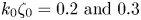$k_0\zeta _0 = 0.2 \text { and } 0.3$) coincide with the BEM$\nu$ results, cf. figures 18 and 19(a,b). The distributions of $\tilde {\mathscr {H}} (x,t)$ elicited from the VOF simulations for breaking wave trains with $k_0\zeta _0 \geq 0.4$ are presented in figure 19(c–f). Similar to the BEM$\nu$ computations, the evolution of non-breaking and weakly breaking wave trains consists of both dispersive focusing and defocusing stages, while there is no clear defocusing stage for strongly breaking cases in the domain of interest, cf. figures 18 and 19. At the same time, the wave train boundaries obtained by the VOF model become rough with the intensification of breaking.

Figure 19. As in figure 18 for VOF model. Dashed and dash-dotted lines show $X_H(t)$ calculated from BEM$\nu$ and VOF simulation results, respectively.

The wave train trajectories $X_H(t)$ (4.23) obtained by the VOF model are plotted in figure 19 with dash-dotted lines. Corresponding plots of $X_H(t)$ taken for reference from figure 18 (BEM$\nu$) are shown by dashed lines. In the focusing stage, the trajectories of weakly breaking wave trains computed by the BEM$\nu$ and VOF models are very close to each other as shown in figure 19(c). Once breaking is initiated in the vicinity of the focal point, see locations depicted by white solid lines in the figure, a small divergence of the trajectories appears. Note that such a deviation in trajectories is not seen prior to the first breaking event. For strong-breaking events as shown in figure 19(d–f), the divergence in wave trajectory between the VOF and BEM$\nu$ models becomes appreciably large. Wave trains computed by the VOF model propagate over longer distances and thus have higher propagation speeds compared with the BEM$\nu$ outcomes. These observations confirm our initial assumption that breaking can increase the propagation speed of wave trains compared with non-breaking scenarios. And this is associated with the phase shifting phenomenon as demonstrated in (4.20).

Applying linear regression to the trajectories $X_H(t)$ derived from BEM$\nu$ and VOF computations, the wave group propagation velocity $v(t) = \textrm {d} X_H / \textrm {d} t$ is estimated numerically and plotted in figure 20. The linear group velocity $c_{g0}$ calculated by using the carrier frequency is included here for reference. Strongly nonlinear but non-breaking wave trains (${\hat {F}_{\hat {x}} \approx 0}$) propagate at a speed moderately higher than the linear group velocity $c_{g0}$. The growth of propagation speed in this case is caused by the nonlinear resonant interaction between spectral harmonics. A similar outcome has been obtained analytically by Stuhlmeier & Stiassnie (Reference Stuhlmeier and Stiassnie2019) for nonlinear waves of Pierson–Moskowitz spectra. Significant increases in the propagation speed can be clearly seen for the breaking waves ($\hat {F}_{\hat {x}}>0$), which may attain the following values: $v_{\textrm {BEM}\nu } \approx 1.27 c_{g0}$ and $v_{\textrm {VOF}} \approx 1.36 c_{g0}$. While the growth observed in BEM$\nu$ computations is mostly related to the nonlinearities in the free-surface boundary conditions (2.2) and (2.3), the additional increment of speed present in the VOF model is likely caused by breaking-induced rotational flows.

Figure 20. (a) Dependence of the wave train propagation velocity $v(t) = \textrm {d} X_H / \textrm {d} t$ on the energy dissipation rate $\hat {F}_{\hat {x}}$ (i.e. wave breaking strength). Dashed and dash-dotted lines represent the linear fit of the data derived from BEM$\nu$ and VOF computations. Mean values of the spectral-weighted group velocities (4.4) obtained from the BEM$\nu$ simulations are plotted for the wave train evolution before and after the linear focus ($t < t_f$ and $t > t_f$). (b) Variation of the spectral-weighted group velocities (4.4) with time obtained for the wave trains of different steepness $k_0 \zeta _0$ using the BEM$\nu$ model.

It is known that the balance of spectral energy in wave forecasting models is closely dependent on wave group velocity, which is usually approximated by the linear dispersion relation (2.13). Stuhlmeier & Stiassnie (Reference Stuhlmeier and Stiassnie2019) pointed out that a more accurate nonlinear approximation of group velocity derived from the Zakharov equation is needed. This means that the complex effect of wave breaking on group velocity is of practical importance and needs to be taken carefully into account.

Next, numerical results collected in the work are used to assess the validity of the spectral-weighted group velocity given by (4.4). The time series of $c_{gs}$ calculated by the BEM$\nu$ model for all the wave trains are depicted in figure 20(b). A gradual growth of $c_{gs}$ is observed within the focusing stage for $t < t_f$ ($t_f = 35\,\textrm {s}$) due to energy downshifting in the spectrum, see figure 12. It is interesting to see that the overall net change of $c_{gs}$ becomes less pronounced after passing the linear focal point for each case. Since the spectra predicted by the BEM$\nu$ and VOF models are close to each other, the values of $c_{gs}$ calculated by these two models are similar to each other. Taking this into account, we estimate the mean values of $c_{gs}$ for the focusing and defocusing stages separately, i.e. $\overline {c_{gs}} |_{t < t_f}$ and $\overline {c_{gs}} |_{t > t_f}$, see figure 20(a). As one can see, the estimates of $\overline {c_{gs}}$ for non-breaking and weakly breaking wave trains are close to the centroid velocity $v(t)$. A large increase in breaking strength can cause $\overline {c_{gs}}$ to deviate significantly from the centroid velocity in the focusing stage. Meanwhile $\overline {c_{gs}}$ is close to $v_{\textrm {BEM}\nu }$ in the defocusing stage. Both estimates do not reflect the wave train propagation velocity computed by the VOF model as expected, since the derivation and calculation of $c_{gs}$ are based on the linear assumption of all the wave components in the spectrum. Despite the deficiency of the spectral-weighted wave train propagation velocity, it can produce sufficiently accurate estimation of energy flux for numerical simulations or experimental measurements, see figure 9(b) and the expression (4.3). Note that we calculate energy fluxes for the VOF model with the expression (4.1) without introducing any simplifications.

Figure 21 exhibits the temporal evolution of wave group length $L_H$, which is defined as the distance between the leading and trailing edges of a wave train, as shown in figures 18 and 19. The wave group length is normalised by its value taken at ${t=30 \,\text {s}}$ when wave generation is completed in both BEM$\nu$ and VOF models. As discussed above, all the non-breaking and weakly breaking wave trains (${0.2 \leq k_0\zeta _0 \leq 0.4}$) are subject to consequent focusing and defocusing stages due to dispersion. For strongly breaking waves with ${k_0\zeta _0 \geq 0.6}$, the defocusing stage is suppressed, cf. figures 21(a) and 21(b). More importantly, the relative wave packet lengths after focusing are nearly constant and have similar magnitude in both BEM$\nu$ and VOF computations: $L_H / L_{H0} = \text {const} \in [0.45, 0.5]$. Wave packet spreading is expected to resume after the breaking process is completed. However, the absolute values of wave group length computed by the BEM$\nu$ and VOF models are different because of the wave evolution peculiarities during the focusing stage.

Figure 21. Evolution in time of the normalised length of the non-breaking to strongly breaking wave trains: (a) BEM$\nu$ and (b) VOF computations. Definition of the wave train length is shown schematically in figures 18 and 19; $L_{H0}$ is the initial wave train length.

It has been reported that wind has a pronounced height amplification effect on broad-banded focusing wave groups in the defocusing stage (Touboul et al. Reference Touboul, Kharif, Pelinovsky and Giovanangeli2008; Chambarel, Kharif & Kimmoun Reference Chambarel, Kharif and Kimmoun2010). It is also of interest and importance to analyse the height amplification effect of wave breaking through the non-dimensional factor given by

(4.24)\begin{equation} \tilde{H}(t) =\frac{2 \times \underset{x}{max} \{ \mathscr{H}(x,t) \}} {H_S(k_0\zeta_0 = 0.4)}.\end{equation}

Here, we introduce the normalisation by using the constant significant wave height $H_S$ calculated for the wave train at the verge of stability, i.e. weakly breaking group with $k_0\zeta _0 = 0.4$. Following the standard definition (Babanin et al. Reference Babanin, Waseda, Kinoshita and Toffoli2011), significant wave height can be calculated from (2.15)

(4.25)\begin{equation} H_S \equiv 4 \sqrt{\frac{1}{2{\rm \pi}}\int_{-\infty}^{+\infty} \hat{\eta}^2(\omega) \,\textrm{d}\omega} = \sqrt[4]{\frac{8}{\rm \pi}} \sqrt{m \zeta_0^2 T_0 \left( 1 + \exp({-2 {\rm \pi}^2 m^2})\right)}.\end{equation}

The factor of $2$ is introduced into the numerator of (4.24) to evaluate the expected wave height from the envelope $\mathscr {H}$. Figure 22 shows the temporal evolution of wave height amplification factor defined by the expression (4.24). Linear regression is applied in panel (b) separately to the focusing ($t < 35\,\text {s}$) and defocusing ($t > 35\,\text {s}$) stages. It is clearly shown that the amplification of the non-breaking wave group ($k_0\zeta _0 = 0.2$) is nearly symmetric about the focal point. An increase in the steepness parameter $k_0\zeta _0$ causes certain asymmetry of $\tilde {H}$ in the pre- and post-focusing stages, see (a).

Figure 22. Evolution of the amplification factor $\tilde {H}$ (4.24) observed in BEM$\nu$ and VOF computations: (a) non- and weakly breaking wave trains, (b) strongly breaking wave trains. Dashed lines present the raw data derived from the computations, while solid lines are obtained by the linear interpolation of the plots separately at focusing and defocusing stages. Vertical dotted line shows focal point location at $t = 35\,\text {s}$.

It is usually expected that strong breaking leads to an instantaneous reduction of wave height. However, figure 22 demonstrates a quite opposite and non-trivial phenomenon. The height amplification factors of strongly breaking wave groups, in particular the solution for $k_0\zeta _0 \ge 0.6$, decay much slower than the non-breaking and weakly breaking ones, cf. (a,b). This is probably due to the suppression of defocusing and the consequent conservation of wave train length shown in figure 21. Both VOF and BEM$\nu$ models demonstrate asymmetry of $\tilde {H}$ plots in the pre- and post-focusing stages with the increase of wave steepness especially when breaking is initiated. The wave train dynamics observed in the BEM$\nu$ model is predominantly governed by the nonlinear wave interactions in the field, see discussion in § 4.4 and Appendix C. On the contrary, the wave train characteristic detected by the VOF model is appreciably different from the BEM$\nu$ solution. This implies that important physical effects are not reflected in the quasi-potential approximation.

Under strong-breaking conditions, see (b), the peak values of $\tilde {H}$ produced by the BEM$\nu$ model are higher than the VOF calculations for each wave train. Unlike the BEM$\nu$ model which shows significant decay rate of $\tilde {H}$ in the post-focusing stage regardless of wave train steepness, the VOF solutions demonstrate a very mild decay of $\tilde {H}$ over time for $k_0\zeta _0 \ge 0.6$. The implication of this phenomenon is that the space (range of $x$) where extreme waves are likely to appear might be larger in VOF simulations than FNP computations. For very steep wave trains $k_0\zeta _0 \ge 0.8$, their amplification factors remain above $2.2$ for a relatively long time in the post-focusing stage as shown in figure 22(b). This can increase the occurrence probability and lifespan of extreme waves.

The change of wave dispersion as well as the conservation of height amplification factor recorded in our simulations are probably caused by breaking-induced rotational flows. These rotational motions are disregarded in the FNP model. According to Rapp & Melville (Reference Rapp and Melville1990), the velocity field of breaking-induced flows consists of the contributions from the mean current, reflected and random waves, turbulence, etc. All of these contributions can be of significance as shown in figure 7. Decomposing the complex velocity field into various components mentioned above is not trivial but actually hardly feasible yet. To accomplish velocity decomposition, it requires substantial theoretical and numerical studies that are beyond the scope of the present work. Nevertheless, following the discussion of Longuet-Higgins (Reference Longuet-Higgins1992) it is probably reasonable to hypothesise that breaking-generated currents are dominant here. This is evident in the proposed empirical expression (4.19), which correlates the change of wave dispersion with the generation of rotational flows. Our calculations show that even a small value of $\tilde {U} \approx 5 \times 10^{-2} c_{g0}$ can cause a significant effect as shown in table 4 and figure 17. Therefore it is probably reasonable to infer that breaking waves interact with the induced currents in a two-way mechanism: breaking can produce currents, in turn the currents can influence the waves by suppressing the dispersion and maintaining the existence of steep waves for a longer time. An extensive theoretical study will be needed to carefully examine the hypothesis. The method of Shrira (Reference Shrira1993) probably needs to be implemented for this task. To accomplish this task, a new method that can be used to decompose the velocity field should be developed. We would like to point out that the duration of a single breaking event, crucial for predictive oceanographic models (Kleiss & Melville Reference Kleiss and Melville2010), is also an important topic requesting further attention.