


1. Introduction
Vortex shedding is a known phenomenon observed in the wake of surface-mounted finite-height square prisms, a type of finite prism where one of its ends (the junction) is mounted on a surface, and the other end (the free end) is subject to flow separation. Figure 1 presents a schematic of a surface-mounted finite-height square prism of aspect ratio  $AR=H/D$, where $H$ is the height of the prism and $D$ is its width, subjected to an incoming free stream flow velocity $U_\infty$ normal to one of the prism's faces (i.e. flow angle of incidence $\alpha =0^\circ$). The surface on which the prism is mounted is defined as the ground plane, where a boundary layer of thickness $\delta$ at $x/D=0$ (the centre of the prism) is formed.

Figure 1. Schematic of a surface-mounted finite-height square prism of width  $D$ and height $H$, subjected to an incoming flow field with free stream velocity $U_\infty$ normal to one of the prism's faces. The prism is partially immersed in a boundary layer of thickness $\delta$. Also defined is the Cartesian coordinate system where $x$,
$x$,  $y$ and $z$ are the streamwise, transverse and vertical coordinates, respectively.
Compared with two-dimensional or ‘infinite’ square prisms, for which alternate or antisymmetric von Kármán vortex shedding is observed in the wake (e.g. Lyn et al. Reference Lyn, Einav, Rodi and Park1995), vortex shedding may suffer disruptions in the wake of surface-mounted finite-height square prisms, due to the three-dimensionality introduced by the free end and the junction. For surface-mounted finite-height prisms with  $AR>2$ (Porteous, Moreau & Doolan Reference Porteous, Moreau and Doolan2017), the currently accepted model of the flow dynamics in their wake is the half-loops (figure 2a) and full-loops (figure 2b) model of Bourgeois, Sattari & Martinuzzi (Reference Bourgeois, Sattari and Martinuzzi2011) and Hosseini, Bourgeois & Martinuzzi (Reference Hosseini, Bourgeois and Martinuzzi2013). In this model, the wake features a periodic alternate shedding of a chain of half-loop structures for dipole-type wakes, defined by the presence of a pair of large time-averaged streamwise vorticity regions that extend into the wake. An additional pair of large streamwise vorticity regions, called base vortices, appears in the lower part of the wake for thicker boundary layers and/or larger $AR$ (Wang et al. Reference Wang, Zhou, Chan and Lam2006; Behera & Saha Reference Behera and Saha2019; Yauwenas et al. Reference Yauwenas, Porteous, Moreau and Doolan2019; Chen et al. Reference Chen, Li, Sun and Liang2022), characterizing the wake as a quadrupole type with the alternate shedding of full loops. The loops are composed by mostly streamwise strands, connected to a vertical core that resembles a Kármán vortex. In the near wake, instances of symmetric coexisting vortices may take place (Sattari, Bourgeois & Martinuzzi Reference Sattari, Bourgeois and Martinuzzi2012), triggered by a low-frequency instability of approximately 0.1 times the dominant shedding frequency (Uffinger, Ali & Becker Reference Uffinger, Ali and Becker2013; Kindree, Shahroodi & Martinuzzi Reference Kindree, Shahroodi and Martinuzzi2018; Peng et al. Reference Peng, Wang, Zeng and He2019; Wang & Lam Reference Wang and Lam2021). This instability has been connected to the drift or shift mode of surface-mounted finite-height square prisms (Bourgeois, Noack & Martinuzzi Reference Bourgeois, Noack and Martinuzzi2013).

Figure 2. Main models of the dynamic flow around a surface-mounted finite-height square prism. (a) Half-loop model of Bourgeois et al. (Reference Bourgeois, Sattari and Martinuzzi2011) and (b) full-loop model of Hosseini et al. (Reference Hosseini, Bourgeois and Martinuzzi2013).
For the case of a surface-mounted cube and other prisms below a critical aspect ratio  $AR_{cr}=2$–4.5, depending on $\delta /D$ (Sakamoto & Arie Reference Sakamoto and Arie1983; Wang et al. Reference Wang, Zhou, Chan, Wong, Lam, Behnia, Lin and McBain2004; McClean & Sumner Reference McClean and Sumner2014; Heng & Sumner Reference Heng and Sumner2020), the symmetric shedding of arch vortices was first proposed to take place (Sakamoto & Arie Reference Sakamoto and Arie1983; Wang & Zhou Reference Wang and Zhou2009). However, this flow model was later challenged in other studies. For example, Shah & Ferziger (Reference Shah and Ferziger1997) found the symmetric arch vortex to be present only in the time-averaged wake of a surface-mounted cube, with a staggered configuration in the instantaneous flow. Hwang & Yang (Reference Hwang and Yang2004) and Schröder et al. (Reference Schröder, Willert, Schanz, Geisler, Jahn, Gallas and Leclaire2020) observed hairpin vortices being shed from the top and lateral leading edges of the cube. A multiscale dynamic flow was recently reported by Li et al. (Reference Li, Rinoshika, Han, Dong, Zheng and Rinoshika2023), where large-scale asymmetric structures were found simultaneously with smaller, mostly symmetric structures that merged and broke down.
On the other hand, no dominant vortex shedding frequency was detected in the wake of prisms with  $AR<2$ by Porteous et al. (Reference Porteous, Moreau and Doolan2017) and with $AR=1$ by Heng & Sumner (Reference Heng and Sumner2020) and Schröder et al. (Reference Schröder, Willert, Schanz, Geisler, Jahn, Gallas and Leclaire2020), suggesting that vortex shedding may have been suppressed. Despite the absence of a spectral peak, downstream-inclined vortex filaments were educed by Porteous et al. (Reference Porteous, Moreau and Doolan2017) in the wake of a prism with $AR=1.4$. The shape of these filaments is similar to the one of the large streamwise structures educed in da Silva, Sumner & Bergstrom (Reference da Silva, Sumner and Bergstrom2022b) from the phase-averaged wake of a cube. The streamwise structures were found to be shed alternately with a Strouhal number $St=f\,D/U_\infty =0.08$ (where $f$ is the shedding frequency), but they were different from the half-loops of taller prisms, due to the absence of a vertical core. The shedding of streamwise structures agrees with the presence of dipole structures (or tip vortices) in the mean wake of a surface-mounted cube, verified in da Silva et al. (Reference da Silva, Hahn, Sumner and Bergstrom2022a). The study in da Silva et al. (Reference da Silva, Sumner and Bergstrom2022b) was, however, limited to the wake of the cube outside the recirculation region. The mean flow in the near wake, as well as near the sides and the top of the cube, contains structures and features such as the arch vortex, corner vortices and, for thicker boundary layers, a headband vortex (da Silva, Sumner & Bergstrom Reference da Silva, Sumner and Bergstrom2024), which have not yet been extensively examined in terms of their dynamic behaviour. The same can be said regarding the low-frequency drift mode, whose effects on the wake of a surface-mounted cube warrant further investigation.
Recent advances in the description of the complex dynamics around surface-mounted finite-height square prisms in general stem in part from the increasing use of flow decomposition methods such as the proper orthogonal decomposition (POD), enabled by the increased availability of computational resources and accurate time-resolved techniques. However, the analysis of turbulent and quasiperiodic wake dynamics still presents challenges, particularly when it comes to the interpretation of the extracted flow modes. Improvements over the traditional POD algorithm have been achieved by combining it with Welch's method (Towne, Schmidt & Colonius Reference Towne, Schmidt and Colonius2018) or through the application of filters (Sieber, Paschereit & Oberleithner Reference Sieber, Paschereit and Oberleithner2016). These techniques yield flow modes that are coherent in both space and time, and, therefore, of higher physical relevance, but the performance of these methods and their variants for the flow around surface-mounted finite-height square prisms is still under scrutiny (e.g. Zhang, Ooka & Kikumoto Reference Zhang, Ooka and Kikumoto2021; Mohammadi, Morton & Martinuzzi Reference Mohammadi, Morton and Martinuzzi2023; Zhang et al. Reference Zhang, Zhou, Tse, Wang, Niu and Mak2023).
In addition, not many studies of the flow around surface-mounted cubes systematically account for the effects of different boundary layers on the flow dynamics, which are significant for taller prisms (Chen et al. Reference Chen, Li, Sun and Liang2022; Mohammadi, Morton & Martinuzzi Reference Mohammadi, Morton and Martinuzzi2022). Boundary layer thickness effects are more commonly assessed on variables such as the vortex shedding frequency (Sakamoto & Arie Reference Sakamoto and Arie1983), aerodynamic force coefficients (Sakamoto Reference Sakamoto1985; Heng & Sumner Reference Heng and Sumner2020) and pressure distribution (Heng & Sumner Reference Heng and Sumner2022). Notable studies that examined effects of the boundary layer thickness on the flow field around a surface-mounted cube include the pioneering study by Castro & Robins (Reference Castro and Robins1977), who evaluated velocity profiles and the occurrence of flow reattachment on the free end of the cube for  $\delta /D=0.025$ and 10; Diaz-Daniel, Laizet & Vassilicos (Reference Diaz-Daniel, Laizet and Vassilicos2017), who studied effects of laminar and turbulent boundary layers on the mean flow and spectral signatures at low Reynolds numbers; and da Silva et al. (Reference da Silva, Sumner and Bergstrom2024) who documented the different mean flow features around the cube for a thin and laminar boundary layer and a thick and turbulent boundary layer. A special mention goes to Porteous, Moreau & Doolan (Reference Porteous, Moreau and Doolan2019), who considered effects of turbulent boundary layers with $\delta /D=1.3$ and 3.7 on the flow-induced noise for $AR=1.4$. However, aside from vortex shedding frequency analyses, these studies considered boundary layer thickness effects on the mean flow field only, highlighting a gap in the literature concerning boundary layer effects on the flow dynamics for very small $AR$.
$AR$.
Therefore, the purpose of the present study is to thoroughly describe the large-scale flow dynamics around a surface-mounted cube, which include the dominant vortex shedding mechanisms and the low-frequency drift mode. In addition, the investigation in da Silva et al. (Reference da Silva, Sumner and Bergstrom2024) will be extended to examine effects of a laminar boundary layer with  $\delta /D=0.2$ and a turbulent boundary layer with $\delta /D=0.8$ on the dynamic flow. The near wake and near-wall flow field on the cube's faces will be specifically addressed, based on large-eddy simulations (LES) with $\textit {Re}=U_\infty D/\nu =1\times 10^4$ (where $\nu$ is the kinematic viscosity of the fluid). The spectral proper orthogonal decomposition (SPOD) algorithm of Sieber et al. (Reference Sieber, Paschereit and Oberleithner2016) will be applied to study the large-scale flow dynamics, given its flexibility and improvement over the traditional POD.
2. Computational methods
The LES of the flow around a surface-mounted cube has been described in more detail in da Silva et al. (Reference da Silva, Sumner and Bergstrom2024). A summary of the most important aspects of its implementation is presented in this section, followed by a brief description of the SPOD method used in this study. The validity of the present LES for the analysis of dynamic flow features is then considered.
Figure 3 presents the computational domain of the flow around a surface-mounted cube of width  $D=0.06$ m. Its extent is 25 $D$ in the streamwise ( $x$) direction, 15 $D$ in the transverse ( $\kern 1.5pt y$) direction and 9 $D$ in the vertical ( $z$) direction. The origin of the domain is at the centre of the junction of the cube with the ground plane, so that the inlet is located 7.5 $D$ upstream of the cube centre. No-slip boundary conditions are specified on the cube and ground plane; the top and side boundaries have a free-slip condition, and the outlet has a convective outflow condition (where $U_c$ is the convective velocity).

Figure 3. Schematic of the computational domain, highlighting its dimensions and boundary conditions for the velocity field.
Different boundary conditions were set at the inlet depending on the boundary layer, yet both conditions lead to the same cube Reynolds number  $\textit {Re}=U_\infty D/\nu =1\times 10^4$. For the laminar boundary layer, a uniform velocity with $U_\infty =2.5$ m s $^{-1}$ was prescribed, giving $\delta /D=0.2$ at $x/D=0$ as verified at a $y/D$ position away from the cube. For the turbulent boundary layer, $\delta /D=0.8$ was desired at the location of the cube for comparison with the wind tunnel measurements of da Silva et al. (Reference da Silva, Hahn, Sumner and Bergstrom2022a). This condition was achieved by mapping turbulent boundary layer results of a precursor channel simulation onto the lower part ( $z<42$ mm) of the inlet boundary of the present simulation, as described in da Silva et al. (Reference da Silva, Sumner and Bergstrom2024). The resulting turbulent boundary layer thickness of $\delta =45$ mm ( $\delta /D=0.8$) is also close to $\delta =44$ mm ( $\delta /D=0.7$) in da Silva et al. (Reference da Silva, Sumner and Bergstrom2022b), which permits the use of their experimental results to evaluate the performance of the LES. Care must be taken, however, regarding the differences in Reynolds numbers in the present study ( $\textit {Re}=1\times 10^4$) and in da Silva et al. (Reference da Silva, Sumner and Bergstrom2022b) ( $\textit {Re}=7.5\times 10^4$). The mean flow field does not change significantly at this order of magnitude, but Lim, Castro & Hoxey (Reference Lim, Castro and Hoxey2007) observed a small $\textit {Re}$ dependency for fluctuating quantities. This $\textit {Re}$ dependency was, however, relatively small for $\textit {Re}<1\times 10^5$, and it is only expected to affect the level of fluctuations, without changing the large-scale flow structures significantly.
A hexahedral grid with  $6\,731\,160$ elements was used for spatial discretization, concentrated near the cube and ground plane. The wall-normal cell dimension $y_w$ ensured maximum values of $y_w^+=y_w u_\tau /\nu$ (where $u_\tau$ is the friction velocity and $\nu =1.5\times 10^{-5}$ m $^2$ s $^{-1}$) of 0.7 for the ground plane and 1.1 for the cube boundaries, while the maximum values of the cell dimensions in the other directions (i.e. $ x^+$ and/or $ z^+$) were approximately 75 and 60 on the cube and ground plane, respectively. The subgrid-scale stress tensor components of the LES were calculated with the dynamic Lagrangian subgrid-scale model of Meneveau, Lund & Cabot (Reference Meneveau, Lund and Cabot1996). Its good performance in reproducing the mean features of the flow, in combination with the hexahedral grid, was verified in da Silva et al. (Reference da Silva, Sumner and Bergstrom2024).
The simulations were carried out with the OpenFOAM toolbox version 7, using the PISO (pressure-implicit with splitting of operators) algorithm to solve the system of equations. Second-order implicit schemes were used to discretize temporal and almost all spatial terms, except for the transport equations of the integral functions of the dynamic Lagrangian subgrid-scale model, whose advective terms were discretized with a first-order upwind scheme. The maximum Courant–Friedrichs–Lewy number was smaller than 1, based on a fixed time step of  $4\times 10^{-6}$ s. After a quasiperiodic state of the flow was reached, velocity and pressure field data were gathered for application of the SPOD (Sieber et al. Reference Sieber, Paschereit and Oberleithner2016). The fields were sampled in a point cloud uniformly distributed from $x/D=-2$ to 10, $y/D=-2.5$ to 2.5 and $z/D=0$ to 3, with a spatial resolution of 0.05 $D$ (3 mm) and at a rate of 100 Hz, during 10 s of flow time (36 or 46 shedding periods). The pressure on the cube's faces and the velocity field at the cells closest to the cube were sampled simultaneously to provide near-wall data. To the improve statistical convergence of the SPOD (Schmidt & Colonius Reference Schmidt and Colonius2020), the spatially distributed data fields were decomposed into their symmetric and antisymmetric components before application of the SPOD, following (2.1) for $u$,
$u$,  $w$ and $p$, and (2.2) for $v$:
$v$:
 \begin{gather} \left.\begin{array}{ll} u_{symmetric}(x,y,z,t)= \dfrac{u(x,y,z,t) + u(x,-y,z,t)}{2}, \\ u_{antisymmetric}(x,y,z,t)= \dfrac{u(x,y,z,t) - u(x,-y,z,t)}{2}, \end{array}\right\} \end{gather}
 \begin{gather} \left.\begin{array}{ll} v_{symmetric}(x,y,z,t)= \dfrac{v(x,y,z,t) - v(x,-y,z,t)}{2}, \\ v_{antisymmetric}(x,y,z,t)= \dfrac{v(x,y,z,t) + v(x,-y,z,t)}{2}. \end{array}\right\} \end{gather}
2.1. Spectral proper orthogonal decomposition
The velocity and pressure fields obtained in the LES, after decomposed, were subjected to the SPOD algorithm of Sieber et al. (Reference Sieber, Paschereit and Oberleithner2016). It consists of a modification on the traditional POD, implemented in this study following the method of snapshots of Sirovich (Reference Sirovich1987), based on a MATLAB script provided by Moritz Sieber.
In the POD and/or SPOD, the fluctuating part of a dataset  $\boldsymbol {u}'(\boldsymbol {x},t)=\boldsymbol {u}(\boldsymbol {x},t)-\bar {\boldsymbol {u}}(\boldsymbol {x})$ is decomposed into a set of $N$ spatial modes $\boldsymbol {\phi }_k(\boldsymbol {x})$ and temporal coefficients ${a}_k(t)$:
 \begin{equation} \boldsymbol{u'}(\boldsymbol{x},t)=\sum_{k=1}^{N} {a}_k(t) \boldsymbol{\phi}_k(\boldsymbol{x}). \end{equation}
Note that the overbar denotes the time average, and the subscript  $k$ refers to a single SPOD mode.
The decomposition is carried out by first computing the correlation matrix  $\boldsymbol {R}$,
 \begin{equation} \boldsymbol{R} = \frac{(\boldsymbol{u}')^{\rm T} \boldsymbol{u}'}{N}, \end{equation}
where  $\boldsymbol {R}$ is a real symmetric matrix of size $N\times N$. In the SPOD, the correlation matrix $\boldsymbol {R}$ is filtered along its diagonals. As explained by Sieber et al. (Reference Sieber, Paschereit and Oberleithner2016), filtering the matrix $\boldsymbol {R}$ increases the similarity along its diagonals, in which periodic patterns in the flow field are found through a wave-like distribution. Therefore, an increased similarity of the dynamics of the underlying signal is obtained as well, and the filter ‘snaps’ to the dominant coherent fluctuations. According to Towne et al. (Reference Towne, Schmidt and Colonius2018), this procedure is equivalent to an interpolation between space-only POD and the purely spectral discrete Fourier transform. The elements of the filtered correlation matrix $\boldsymbol {S}$ are given by (Sieber et al. Reference Sieber, Paschereit and Oberleithner2016)
 \begin{equation} S_{i,j}= \sum_{k={-}N_f}^{N_f} g_k R_{i+k,j+k}, \end{equation}
where  $\boldsymbol {g}$ is a low-pass symmetric impulse response filter of length $2N_f+1$ and $N_f$ is the filter width.
The next steps follow the traditional POD, where the eigenvector matrix  $\boldsymbol {b}$ and eigenvalues $\lambda$ of the matrix $\boldsymbol {S}$ are obtained by solving the eigenvalue problem
 \begin{equation} \boldsymbol{S} \boldsymbol{b}=\lambda \boldsymbol{b}, \end{equation}
where the  $N\times N$ eigenvector matrix $\boldsymbol {b}$ is orthogonal. The eigenvalues and eigenvectors are sorted so that $\lambda _1\geq \lambda _2 \geq \cdots \geq \lambda _N \geq 0$, and each mode's eigenvector $b_k$ is scaled to give the temporal coefficients vector ${a}_k(t)$,
 \begin{equation} a_k(t) = b_k \sqrt{N \lambda_k}. \end{equation}
Note that the scaling is applied so that, for any two given modes  $i$ and $j$ (Sieber et al. Reference Sieber, Paschereit and Oberleithner2016),
 \begin{equation} \frac{1}{N} (\boldsymbol{a}_i \boldsymbol{{\cdot}} \boldsymbol{a}_j) = \lambda_i \delta_{ij}, \end{equation}
where  $\delta _{ij}$ is the Kronecker delta and $(\,{\cdot }\,)$ denotes the scalar product. It follows that the temporal coefficients are uncorrelated (Sirovich Reference Sirovich1987).
The spatial modes  $\boldsymbol {\phi }_{k}(\boldsymbol {x})$ are calculated by projecting the fluctuating field onto the temporal coefficients $a_k$ (Sieber et al. Reference Sieber, Paschereit and Oberleithner2016),
 \begin{equation} \boldsymbol{\phi}_{k}(\boldsymbol{x}) = \frac{1}{N \lambda_k} \sum_{j=1}^{N} a_k(t_j) \boldsymbol{u}'(\boldsymbol{x},t_j). \end{equation}
They represent spatial correlations within the flow, where the associated mode energy  $\lambda _k$ is typically related to the turbulent kinetic energy (TKE) of each mode. They are, however, not orthogonal, as a consequence of the filter operation (Sieber et al. Reference Sieber, Paschereit and Oberleithner2016).
The SPOD also allows for the identification of coupled or paired modes, i.e. modes that contain similar spectral content, but shifted by  ${\rm \pi} /2$. As such, they can be combined into a complex-valued mode, able to express the space–time evolution of coherent structures. Sieber et al. (Reference Sieber, Paschereit and Oberleithner2016) propose the identification of coupled modes through the harmonic correlation of their temporal coefficients, obtained from a dynamic mode decomposition of the coefficients.
The strength of the filter operation in the SPOD is controlled through the filter width  $N_f$: if it is equal to zero, the SPOD converges to the POD, and if it is equal to the number of snapshots $N$, the SPOD converges to the discrete Fourier transform (Sieber et al. Reference Sieber, Paschereit and Oberleithner2016). An appropriate choice of $N_f$ allows the SPOD to better separate the spectral contents of the flow field and recover dynamics weaker than the noise level, which are limitations of the classical POD (Sieber et al. Reference Sieber, Paschereit and Oberleithner2016; Mohammadi et al. Reference Mohammadi, Morton and Martinuzzi2023). On the other hand, there is a loss of optimality of the decomposition, and the energy contained by the first (most energetic) modes trickles into higher-ranked modes, especially for a large filter width $N_f$. Therefore, a moderate filter width must be chosen. Sieber et al. (Reference Sieber, Paschereit and Oberleithner2016) recommends the use of characteristic time scales associated with the coherent structures of interest. Perret & Kerhervé (Reference Perret and Kerhervé2019) used a filter width that corresponded to approximately three times their period of interest, and Mohammadi et al. (Reference Mohammadi, Morton and Martinuzzi2023) reported best results for $N_f$ equal to 6.4 times the shedding period for a surface-mounted finite-height square prism with $AR=4$. Based on the literature results and tests for different values of $N_f$ documented in the Appendix, a Gaussian filter with a width of six times the shedding period was adopted in the present analysis.
2.2. Comparison with experimental large-scale flow dynamics
While the performance of the LES was scrutinized in da Silva et al. (Reference da Silva, Sumner and Bergstrom2024) concerning the mean flow field, the suitability of the present results to represent the large-scale flow dynamics must also be assessed. Instead of considering the SPOD spatial modes by themselves, which may be hard to interpret, the spatial modes will be used to partially reconstruct the flow field, as was done by El Hassan, Bourgeois & Martinuzzi (Reference El Hassan, Bourgeois and Martinuzzi2015), Wang et al. (Reference Wang, Lam, Zu and Cheng2019b), Wang, Cheng & Lam (Reference Wang, Cheng and Lam2019a) and Cao et al. (Reference Cao, Liu, Zhou and Ren2022). In addition, by reconstructing the flow field using the first antisymmetric mode pair, shown in § 3.1 to correspond to the dominant vortex shedding mode, the reconstructed flow field can be compared with the experimental phase-averaged results in da Silva et al. (Reference da Silva, Sumner and Bergstrom2022b) for  $\delta /D=0.7$ and $\textit {Re}=7.5\times 10^4$, shown in figure 4. The reconstructed field with the first antisymmetric mode pair at an instant $t_j$ is given by
 \begin{equation} \boldsymbol{u}(\boldsymbol{x},t_j) = \bar{\boldsymbol{u}}(\boldsymbol{x}) + a_1^A(t_j)\boldsymbol{\phi}_1^A(\boldsymbol{x}) + a_2^A(t_j)\boldsymbol{\phi}_2^A(\boldsymbol{x}), \end{equation}
where the superscript  $A$ indicates the antisymmetric mode. The reconstruction with a symmetric mode would likewise feature a superscript $S$. However, to enable a comparison with the 20 phases of the experimental data, a mean periodic behaviour was fitted from the SPOD coefficients by deriving new coefficients from sine and cosine functions with the mean peak amplitude of the SPOD coefficients $a_1^A$ and $a_2^A$. A phase increment of $3{\rm \pi} /10$ was used to reproduce phases 1, 4, 7 and 10 of da Silva et al. (Reference da Silva, Sumner and Bergstrom2022b), and the first phase was arbitrarily selected.

Figure 4. Phase-averaged or reconstructed velocity components using the first SPOD antisymmetric mode pair for the flow around the cube with the turbulent boundary layer, at four instants which approximately correspond to phases 1, 4, 7 and 10 of the cross-wire anemometry (XWA) results of da Silva et al. (Reference da Silva, Sumner and Bergstrom2022b). Velocity components are compared in a line located at (a)  $x/D=4$ and $z/D=0.5$, and (b) $x/D=6$ and $z/D=0.5$.
Profiles of the reconstructed flow field using the first antisymmetric SPOD mode pair obtained from the LES are shown in figure 4 to essentially follow the trends of the experimental data. For the velocity components at  $x/D=4$ and $z/D=0.5$ (figure 4a), the location of the minimum streamwise ( $u/U_\infty$) and vertical ( $w/U_\infty$) velocity component switches from the $-y$ side of the domain to the $+y$ side from phase 1 to phase 10, while the transverse ( $v/U_\infty$) velocity component changes from negative to positive near the centre. The SPOD modes are able to reproduce the same dynamics, but some disagreement is found especially regarding the magnitude of the $u/U_\infty$ component near the centre. The LES/SPOD gives a wider region of low $u/U_\infty$ and a lower minimum velocity. The latter may be due the limitations of the XWA method near regions of turbulent reverse flow, in which the measured mean velocity may be artificially increased. This is not an issue at $x/D=6$ and $z/D=0.5$ (figure 4b), which is farther from the reverse-flow region, and the LES/SPOD results follow the experimental data more closely. At both locations, the vertical component is lower than in the experimental results away from the centre, a characteristic also present in the mean flow field (da Silva et al. Reference da Silva, Sumner and Bergstrom2024).
As observed previously, the level of fluctuations in the flow field may change depending on the Reynolds number, a behaviour that must be considered since the present  $\textit {Re}=1\times 10^4$ is smaller than $\textit {Re}=7.5\times 10^4$ in da Silva et al. (Reference da Silva, Sumner and Bergstrom2022b). To this end, the Reynolds stresses contributed by the first antisymmetric SPOD mode pair have been calculated and averaged over the same $y$–
$y$– $z$ planes at $x/D=4$ and $x/D=6$ of da Silva et al. (Reference da Silva, Sumner and Bergstrom2022b). Their contribution to the total (time-averaged) Reynolds stresses is presented in table 1, where, for the shear stresses, the average was calculated over their absolute local values (the $\overline {v'w'}$ stress was not included since it was not measured experimentally).
Table 1. Contribution of the area-averaged Reynolds stresses of the first antisymmetric mode pair to the total area-averaged Reynolds stresses in the  $y$–
$y$– $z$ planes at $x/D=4$ and 6, compared with the contribution of the periodic stresses in the XWA data of da Silva et al. (Reference da Silva, Sumner and Bergstrom2022b). For the shear stresses, averages were calculated over the absolute values of the points.

Similar levels are observed in table 1 for the contribution of the main antisymmetric mode pair and the periodic component of the phase-averaged flow field. The absolute differences are within 5 % in all cases, with the highest discrepancy observed for the  $\overline {u'u'}$ component at $x/D=4$, where the higher probability of reverse flow increases the experimental uncertainty. Despite small disagreements that may be attributed to experimental uncertainty, numerical uncertainty and Reynolds number differences, the present assessment shows that the most energetic SPOD modes obtained with the LES are capable of describing the important features of the dominant large-scale shedding dynamics, and contribute fluctuations at approximately the same level.
3. Results and discussion
The SPOD modes and eigenvalues obtained for the flow around a surface-mounted cube will be briefly presented in § 3.1, for the laminar boundary layer with  $\delta /D=0.2$ (also referred to as ‘thin’) and the turbulent boundary layer with $\delta /D=0.8$ (also referred to as ‘thick’). Then, the flow dynamics will be scrutinized in terms of the main antisymmetric vortex shedding mode in § 3.2 and the symmetric drift mode in § 3.3, which are the most relevant modes for the analysis of the large-scale flow dynamics around the surface-mounted cube.
3.1. Spectral proper orthogonal decomposition overview
As mentioned in § 2.1, a filter width of six vortex shedding periods was chosen for the application of the SPOD to the flow field data. The shedding period was verified based on the spatially averaged spectra of the velocity components, shown in figure 5. For the thin boundary layer,  $St=0.113$ (or $f=4.7$ Hz) was obtained, versus $St=0.086$ (or $f=3.6$ Hz) for the thick one, both of which agree with experimental measurements (Sakamoto & Arie Reference Sakamoto and Arie1983). Other minor peaks are present in the spatially averaged spectra due to the quasiperiodic nature of the flow around the cube, especially for the turbulent boundary layer. A notable energy concentration is found at a lower dimensionless frequency band highlighted as $f_d D/U_\infty \approx 0.01$ in figure 5, for both cases. This frequency band corresponds to the low-frequency drift of the wake, at approximately 1/10th of the vortex shedding frequency.

Figure 5. Spatially averaged power spectral density (PSD) of the velocity components for the flow around the surface-mounted cube with (a)  $\delta /D=0.2$ and (b) $\delta /D=0.8$.
The most-energetic spatial modes obtained with the SPOD of the antisymmetric and symmetric components of the flow field are presented in figure 6. Note that the modes are presented individually, but a high harmonic correlation was obtained between the first and second antisymmetric modes and between the first and second symmetric modes, characterizing each of them as a pair. In addition, energy contributions were computed as a ratio to the total energy (added from the symmetric and antisymmetric decompositions), since its additive property is ensured by the orthogonality of symmetric and antisymmetric vectors fields (Bourgeois et al. Reference Bourgeois, Noack and Martinuzzi2013). A convective pattern is found for the first antisymmetric mode pair for both boundary layers (figure 6a i,a ii,b i,b ii), characterizing this first pair as a shedding mode. For the thin boundary layer, the first mode pair has  $St=0.113$ and the highest contribution to the total TKE, of 16.1 % (figure 6c) based on its eigenvalues, which confirms it as the dominant vortex shedding mode. The same is observed for the thick boundary layer (figure 6d), although with an overall lower contribution of the mode pair to the TKE energy, of 4.0 %. This lower contribution is expected for turbulent boundary layers, where the energy is transferred to higher-order modes (El Hassan et al. Reference El Hassan, Bourgeois and Martinuzzi2015). In comparison with the thin boundary layer, the structures in the antisymmetric modes for the thick boundary layer are more elongated, in line with their lower shedding frequency; the implicated dynamics will be further discussed in § 3.2.

Figure 6. Contours of the spatial SPOD modes  $\phi _k$ in $x$–
$x$– $y$ planes at $z/D=0.5$ (midheight), for the first antisymmetric and symmetric mode pairs for (a) $\delta /D=0.2$ and (b) $\delta /D=0.8$. The PSD of the temporal coefficients of the first antisymmetric and symmetric modes are presented in (c,d), respectively.
The most energetic symmetric mode pair (figure 6a iii,a iv,b iii,b iv) shows a non-convective pattern and temporal coefficient spectra with high energetic contents around the drift frequency  $f_d$, confirming this pair as the low-frequency drift mode of the wake for both boundary layers. This mode accounts for a small portion of the total TKE, with 2.2 % and 1.0 % for the thin and thick boundary layers, respectively. Even so, the drift mode affects the entire near wake, in agreement with Wang & Lam (Reference Wang and Lam2021), showing a stronger influence for the thin boundary layer case. The effects of this instability are considered in detail in § 3.3.
Other higher-order modes which are not discussed in detail in this study but which are documented in the Appendix include the second harmonic of the vortex shedding mode and accompanying shedding modes. The second harmonic of the vortex shedding mode appears as a symmetric mode pair with  $f\,D/U_\infty =2St$, which contributes 0.7 % and 0.6 % of the TKE for the thin and thick boundary layers, respectively. The accompanying shedding mode pairs are the second most energetic antisymmetric modes, with mode shapes similar to those of the dominant shedding modes. The spectra of their temporal coefficients show two peaks, at a higher and a lower frequency than the vortex shedding frequency, referred to as accompanying frequencies by Kindree et al. (Reference Kindree, Shahroodi and Martinuzzi2018). These frequencies were proposed to be related to the interaction between the free end and the Kármán-like vortices (Mohammadi et al. Reference Mohammadi, Morton and Martinuzzi2023), and are given by $f_{ai} D/U_\infty =St\pm f_d D/U_\infty$ (Kindree et al. Reference Kindree, Shahroodi and Martinuzzi2018).
3.2. Antisymmetric vortex shedding
An overview of the main antisymmetric vortex shedding mode is shown in figure 7. The flow field has been reconstructed following (2.10) at four sequential instants  $t_1$, $t_2$, $t_3$ and $t_4$, which span approximately one half of a high-amplitude shedding cycle. The vorticity and $\lambda _2$ fields have been spatially filtered with a Gaussian filter of width $0.1D$ to eliminate noise and highlight the most important structures, and the flow field is shown as seen from the $-y$ side and from the top, at each instant. The dynamics associated with this flow reconstruction are also shown in supplementary movie 1 available at https://doi.org/10.1017/jfm.2024.551 for the thin boundary layer and supplementary movie 2 for the thick boundary layer.

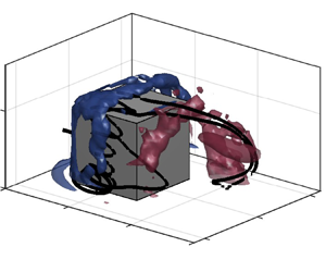
Figure 7. Isosurfaces of  $\lambda _2 D^2/U_\infty ^2=-0.05$ coloured by the streamwise vorticity $\omega _x D/U_\infty$ for the flow reconstructed with the first antisymmetric mode pair at four instants indicated by the circles at the top of the figure. Here (a) $\delta /D=0.2$ and (b) $\delta /D=0.8$; $T_1^A$ denotes the period corresponding to the dominant frequency identified for the first antisymmetric mode.
Figure 7 shows that all the major mean flow structures around the cube – the horseshoe vortex, the arch vortex and the dipole structures – are affected by the dominant shedding mode. The wake is composed of the alternate shedding of mostly streamwise structures, akin to the streamwise strands of the half-loops characteristic of taller surface-mounted finite-height square prisms which are responsible for the appearance of the time-averaged dipole. Instant  $t_1$ shows, for both boundary layers, the shedding of a structure S1 that features a strong clockwise (CW) (blue) streamwise vorticity component. This instant features a longer horseshoe vortex leg on the $-y$ side of the wake, also characterized by CW (blue) streamwise vorticity. As S1 travels downstream at instant $t_2$, it also extends outward in the $-y$ direction, contrary to the preceding structure S0, which contains anticlockwise (ACW) (orange) streamwise vorticity. The arch vortex is staggered, in agreement with Shah & Ferziger (Reference Shah and Ferziger1997), with its $+y$ side located farther from the cube at this instant. At $t_3$, S1 is released and a new structure S2, with a strong ACW (orange) streamwise vorticity component, starts being formed from the $+y$ side of the arch vortex. The horseshoe vortex leg on the $-y$ side of the wake retracts, after shedding part of it with S1. The structure S2 continues its development at $t_4$, at the same time that the horseshoe vortex leg on the $+y$ side extends and the arch vortex leg on the $-y$ side starts to advance.
Regarding the nature of the shed structures, half-loops are formed only for the thin boundary layer case and at the beginning of the shedding process – for example, structure S1 at  $t_1$ in figure 7(a). As the structures travel downstream, they lose their small vertical core and become mostly streamwise structures. With the thick boundary layer, no vertical core is formed in agreement with da Silva et al. (Reference da Silva, Sumner and Bergstrom2022b). The arch and streamwise vortices are overall weaker for the thick boundary layer, as is the case for the flow around taller prisms with turbulent boundary layers (Mohammadi et al. Reference Mohammadi, Morton and Martinuzzi2022), and the streamwise structures are initially composed of two combined strands: one central and one external, as shown for S1 at $t_1$ in figure 7(b). These two strands are also apparent for the thin boundary layer, but the separation between them is much less pronounced. Despite these differences, both boundary layers share a similar formation mechanism of the streamwise structures. A closer view of the near wake at instant $t_1$ is presented in figure 8. The velocity streamlines further show that S1 emerges from within the arch vortex, suggesting that these structures are formed from the reorientation of the arch vortex's vorticity.

Figure 8. Close-up of instant  $t_1$ in figure 7, with three-dimensional streamlines of the velocity field seeded in the vicinity of structure S1. Here (a) $\delta /D=0.2$ and (b) $\delta /D=0.8$.
To further investigate this hypothesis, the transport of the resolved streamwise vorticity component was considered for the SPOD reconstruction. A similar analysis was carried out by Tu et al. (Reference Tu, Wang, Gao, She, Wang, Wang and Wei2023) for a surface-mounted hemisphere and Crane et al. (Reference Crane, Popinhak, Martinuzzi and Morton2022) for a surface-mounted cylinder, where the authors identified that contributions from the stretching and tilting terms were dominant to the mean flow field and could be considered the main mechanism of vorticity transport. The same was verified in the present results, with mean stretching and tilting contributing 40 % and 39 % of the total streamwise vorticity transport over the sampled volume for the thin and thick boundary layers, respectively. Higher relative contributions are expected for the stretching and tilting of the reconstructed vorticity field due to the inclusion of the coherent fluctuations from vortex shedding.
The stretching and tilting terms for the streamwise vorticity are, respectively, defined as
 \begin{gather} S_x = \omega_x \frac{\partial u}{\partial x}, \end{gather}
 \begin{gather}T_x = \omega_y \frac{\partial u}{\partial y} + \omega_z \frac{\partial u}{\partial z}. \end{gather}
A positive value of the stretching and tilting terms denotes the generation of ACW streamwise vorticity, while a negative value corresponds to generation of CW streamwise vorticity. Figure 9 presents the vorticity components in the near wake of the cube with the laminar boundary layer with  $\delta /D=0.2$, at instant $t_1$ of figure 7, as well as the stretching and tilting terms of the streamwise vorticity. Semitransparent isosurfaces of $\lambda _2$ are included for reference.

Figure 9. Isosurfaces of vorticity components and vorticity transport terms for the reconstructed flow field at instant  $t_1$ of figure 7, for $\delta /D=0.2$. (a–c) Streamwise ( $\omega _x D/U_\infty$), transverse ( $\omega _y D/U_\infty$) and vertical ( $\omega _z D/U_\infty$) vorticity components; (d,e) streamwise stretching ( $S_x D^2/U_\infty ^2$) and tilting ( $T_x D^2/U_\infty ^2$) terms. Positive values of $S_x$ and $T_x$ denote the generation of positive (ACW) $\omega _x$, and negative values correspond to negative (CW) $\omega _x$. The semitransparent grey isosurfaces indicate $\lambda _2 D^2/U_\infty ^2=-0.05$, for reference.
As previously shown in figure 8, the streamwise structure S1 has a strong CW streamwise vorticity component  $\omega _x$, but smaller ACW vorticity regions are found near the ground, characterizing a ground plane vorticity (da Silva et al. Reference da Silva, Sumner and Bergstrom2024) that follows structure S0, and within the arch vortex. The arch vortex is characterized mainly by a strong transverse vorticity component $\omega _y$ near the top of the structure, and a vertical component $\omega _z$ near the arch vortex's legs. This distribution is a consequence of the rolling-up of the separated shear layers behind the cube. Asymmetries are observed in these vorticity components as well in the present antisymmetric reconstruction, with high-magnitude $\omega _y$ found at the beginning of S1. The region of positive $\omega _z$ is stretched along this structure, which shows its role in the formation of the vertical core of S1. On the other side, the negative $\omega _z$ region is not as long, but it is thicker closer to the cube due to the rolling-up of the shear layer on the $+y$ side – a prelude to the shedding of the next streamwise structure.
Regarding the streamwise stretching and tilting terms in figure 9,  $S_x$ shows a high negative component along S1, consistent with its extension downstream in the wake. The stretching of S1 is found mostly near the end of the recirculation region, where $\partial u/\partial x$ is positive. However, there is a concentration of positive $S_x$ wrapped around the region of negative $S_x$. The positive $S_x$ amplifies the small ACW streamwise vorticity in the arch vortex (to be developed into a new streamwise structure), reduces the generation of CW vorticity towards the $+y$ side of the wake and stretches the ACW vorticity associated with structure S0, near the ground.
The most significant generation of the streamwise vorticity is related to the tilting term,  $T_x$. Within the arch vortex, a net positive $T_x$ is achieved, which contributes to the eventual generation of the streamwise vorticity of structure S2 due to the tilting of both the strong $\omega _y$ and $\omega _z$ components. Right outside the arch vortex, a net negative $T_x$ is responsible for the CW $\omega _x$ of S1. The sign of $T_x$ alternates between positive and negative in the wake due to fluctuations in the strength of both $\omega _y {\partial u}/{\partial y}$ and $\omega _z {\partial u}/{\partial z}$. While both terms are significant to the net $T_x$, the $y$ contribution changes mainly due to variations in the distribution of $\partial u/\partial y$, while the $z$ contribution changes due to variations of $\omega _z$ throughout the shedding cycle. This behaviour is shown in the profiles of the components of $T_x$ at $x/D=2$ and $z/D=0.75$ in figure 10(a) for $t_1$ and $t_4$, which represent approximately opposite phases. At $t_1$, the negative $T_x$ is derived from the higher $\omega _z$ on the $+y$ side of the wake, due to the curling shear layer, and from the strong negative gradient $\partial u/ \partial y$ on the $-y$ side of the wake, which tilts the positive $\omega _y$. The dynamics are reversed at $t_4$, which results in a net positive $T_x$ in this region.

Figure 10. Profiles of  $\partial u/\partial y$, $\partial u/\partial z$, $\omega _y D/U_\infty$, $\omega _z D/U_\infty$ and $T_x D^2/U_\infty ^2$ in a line located at $x/D=2$ and $z/D=0.75$ for the reconstructed flow field at instants $t_1$ and $t_4$, for (a) $\delta /D=0.2$ and (b) $\delta /D=0.8$.
The formation of streamwise structures had been previously explained based on effects of the downwash (da Silva et al. Reference da Silva, Sumner and Bergstrom2022b) or Biot–Savart induction (Mohammadi et al. Reference Mohammadi, Morton and Martinuzzi2022). The present explanation based on vorticity stretching and tilting does not conflict with these approaches; instead, it contributes to the understanding of the formation process through an objective analysis of the dynamic flow field. This process is schematized in figure 11(a) for the thin boundary layer, for the formation of a structure such as S2, characterized by ACW streamwise vorticity. The streamwise structure is shown to branch off from the arch vortex, with the two tilting contributions highlighted in the figure. The streamwise tilting of  $\omega _z$ by $\partial u/ \partial z$ is more prominent in the larger (left-hand) leg of the arch vortex, with the positive $\omega _z$ and $\partial u/ \partial z$ yielding a positive streamwise vorticity at the instant depicted in figure 11. The positive $\omega _x$ of S2 is also a result of the tilting of $\omega _y$ by a strong and positive $\partial u/ \partial y$, at the right-hand side of the wake.

Figure 11. Schematic of the formation process of streamwise structures in the wake of a surface-mounted cube. Here (a)  $\delta /D=0.2$ and (b) $\delta /D=0.8$. The horseshoe vortex has been omitted for clarity.
A similar mechanism takes place for the flow around the cube with the turbulent boundary layer with  $\delta /D=0.8$, for which the vorticity and streamwise stretching and tilting are presented in figure 12. The streamwise vorticity and its stretching and tilting terms are, however, weaker than for the thin boundary layer. The CW streamwise vorticity of structure S1 is discernible, but the ACW vorticity of the budding structure S2 is not, based on the chosen values of $\omega _x D/U_\infty =\pm 1$. Likewise, the positive stretching term $S_x$ is seen only close to the ground plane, in contrast to its significant contribution to the enhancement of positive $\omega _x$ for the thin boundary layer case. The absence of significant positive $S_x$ around S1 may contribute to the reduced displacement of the streamwise structures outward in the wake with the thick boundary layer, in addition to the proximity of the horseshoe vortex, which confines the $\omega _z$ of the lateral shear layers into a narrower wake.

Figure 12. Isosurfaces of vorticity components and vorticity transport terms for the reconstructed flow field at instant  $t_1$ of figure 7, for $\delta /D=0.8$. (a–c) Streamwise ( $\omega _x D/U_\infty$), transverse ( $\omega _y D/U_\infty$) and vertical ( $\omega _z D/U_\infty$) vorticity components; (d,e) streamwise stretching ( $S_x D^2/U_\infty ^2$) and tilting ( $T_x D^2/U_\infty ^2$) terms. Positive values of $S_x$ and $T_x$ denote the generation of positive (ACW) $\omega _x$, and negative values correspond to negative (CW) $\omega _x$. The semitransparent grey isosurfaces indicate $\lambda _2 D^2/U_\infty ^2=-0.05$, for reference.
The  $\partial u/\partial y$ gradient, vertical vorticity component $\omega _z$ and tilting term $T_x$ are overall lower for the thick boundary layer, as shown in figures 10(b) and 12, but $\omega _y$ and $\partial u/\partial z$ have comparable magnitude with the thin boundary layer profiles. In addition, the overlap of the high-magnitude $\omega _y$ with the external strand of S1 in figure 12 suggests that this vorticity component contributes significantly to the formation of this strand, while the central one benefits from the tilting of both $\omega _y$ and $\omega _z$ into the streamwise vorticity characteristic of S1. Based on these features, figure 11(b) depicts the formation process of the streamwise structure S2 for the thick boundary layer, where the external and central strands can be distinguished. The headband vortex – to be further discussed below – is also included for completeness.
Figure 8(b) reveals that the arch vortex is less defined for the thick boundary layer case, as well as the presence of a side vortex on the  $-y$ side of the cube. These features are shown in greater detail in figure 13, where different values of $\lambda _2$ have been selected to highlight the arch vortex in the near wake and the headband vortex around the cube with the thick boundary layer.

Figure 13. Isosurfaces of  $\lambda _2 D^2/U_\infty ^2=-0.7$ (for $x/D\geq 0.5$) and $-$2.5 and streamlines of the velocity field reconstructed with the first antisymmetric mode pair at instant $t_1$ of figure 7. Here (a) $\delta /D=0.2$ and (b) $\delta /D=0.8$.
With the thin boundary layer (figure 13a), the three-dimensional velocity streamlines reveal a corner vortex near the upstream junction of the cube with the ground plane, despite the absence of an isosurface of  $\lambda _2 D^2/U_\infty ^2=-2.5$ near this region. The flow rolls up after the cube, leading to a large arch vortex leg on the $-y$ side of the wake. This arch vortex leg shows a higher intensity of $\lambda _2$ than the one on the $+y$ side of the wake (and in turn is larger in size – see figure 8a, for example), which indicates a stronger vortex core. This is not the case for the flow field with the thick boundary layer (figure 13b), for which the arch vortex leg on the $-y$ side is weaker. In this case, the corner vortex on the side of the cube develops into a side or headband vortex, due to the narrower wake and proximity of the high-momentum flow, which promotes flow attachment on the side and top of the cube. The proximity of the arch vortex leg to the side vortex on the $-y$ side of the wake contributes to its weakening, and may in turn explain the absence of a vertical core in the shed structures with the thick boundary layer, despite the presence of significant $\omega _z$ in the region.
The described flow dynamics of the dominant vortex shedding mode and the different configurations observed for the thin and thick boundary layer cases have implications on the near-wall flow field and pressure distribution on the cube's faces. To evaluate these effects, the flow decomposition into symmetric and antisymmetric components and the SPOD were applied to the pressure and near-wall velocity fields (i.e. the velocity field at the closest cells to the cube, distance 0.0006 $D$), sampled simultaneously with the three-dimensional flow field. Zero weights were applied to the pressure fields, to ensure that the energy of the decomposed modes physically corresponds to contributions to the TKE of the flow. Therefore, the pressure modes obtained from the near-wall fields represent the same physical phenomena, akin to the results of an extended POD (Maurel, Borée & Lumley Reference Maurel, Borée and Lumley2001) as performed in Zhang et al. (Reference Zhang, Zhou, Tse, Wang, Niu and Mak2023). For the thin boundary layer, the temporal coefficients of the main antisymmetric mode pair obtained from this dataset had the same dominant frequency and high correlation ( ${>}0.8$) with the temporal coefficients obtained from the three-dimensional flow field, but with a phase difference of almost one shedding cycle. For the thick boundary layer, the large-scale flow dynamics of the three-dimensional flow field was instead contained in both the first and second antisymmetric mode pairs, so both were included in the reconstruction. The reconstructed pressure coefficient and near-wall velocity fields at the same instant $t_1$ as in figure 7 are presented in figure 14, with the pressure coefficient defined as $C_p=p/(0.5 \rho U_\infty ^2)$. The fields on the front face of the cube are not shown, since it is mostly unaffected by the antisymmetric shedding mode. A few notable critical points are highlighted to facilitate the comparison between the two boundary layers.

Figure 14. Contours of  $C_p$ on the cube's rear, side and top faces and near-wall velocity streamlines for the flow field reconstructed with the (a) first or (b) first and second antisymmetric mode pair at instant $t_1$ of figure 7. Notable node (N, $\square$), focus (F, $\circ$) and saddle (S, $\lozenge$) points are highlighted. Here (a) $\delta /D=0.2$ and (b) $\delta /D=0.8$.
The main antisymmetric shedding mode causes the stagnation point on the rear of the cube, labelled N $_2$ in figure 14, to move side-to-side during the cycle. At $t_1$, the point is found towards the $-y$ direction due to the increased roll-up of the shear layer on the $+y$ side. The limiting streamlines are similar for both boundary layers, but the pressure coefficients show an overall higher magnitude for the thick boundary layer (figure 14b) due to flow attachment on the sides of the cube (Sakamoto Reference Sakamoto1985).
Note that flow attachment also takes place on the sides of the cube with the thin boundary layer, but it is of the backward flow that separates from the cube's rear edges (type B of da Silva et al. (Reference da Silva, Hahn, Sumner and Bergstrom2022a)). A C-shaped attachment line is formed on both sides of the cube in figure 14(a), containing the lateral saddle point  $S_{L}$. The backward near-wall flow then separates at either of the leading edges of the cube or at focus point $F_{c}$, associated with the corner vortex. This pattern is found on both sides of the cube with the thin boundary layer, but the pressure changes significantly: lower pressure coefficients are found on the $-y$ side, where the lateral shear layer is shorter. The same happens on the top face of the cube, regarding the pressure distribution. Type B attachment is found, with the saddle point $S_{t}$ located towards the $-y$ side as well, on the C-shaped attachment line.
For the thick boundary layer (figure 14b), the near-wall flow pattern on the sides of the cube is more complex due to the formation of the headband vortex. Type B attachment also takes place, with the presence of the lateral saddle point  $S_{L}$ over the main attachment line, but the trailing edge bubble is smaller on both sides of the cube in comparison with the thin boundary layer. The pressure shows greater spatial variation on the sides, with higher pressure near the attachment lines. The pressure is again overall lower on the $-y$ side, but with the lowest values close to the focus point $F_{c}$ instead. On the $-y$ side, a well-defined separation line that connects $F_{c}$ and the saddle of separation $S_{s}$ delimits the extent of the side vortex, and an additional attachment line with the node of attachment $N_{a}$ is formed near the leading edges, maintaining topological consistency. This flow distribution is similar to the one for the mean flow field presented in da Silva et al. (Reference da Silva, Sumner and Bergstrom2024), where an alternative visualization of the attachment–separation–attachment pattern in $x$–
$x$– $y$ planes can be found. On the $+y$ side, $S_{s}$ and $N_{a}$ are close to merging, approximating the flow pattern to the one observed for the thin boundary layer case. This behaviour indicates the weakening of the side vortex on this side, which is accompanied by a stronger arch vortex leg as shown in figure 13, in contrast to the strengthened side vortex on the $-y$ side.
The flow pattern on the free end of the cube with the thick boundary layer also shows type B attachment, indicated by the main attachment line that contains  $S_{t}$. Additional critical points are found, however, due to the formation of the headband vortex: the separation saddle point $S_{t2}$ delimits the region over which the top part of this vortex is found, and the node of attachment $N_{t}$ is found near the leading edge. While $S_{t}$ stays closer to $y/D=0$ than for the thin boundary layer, asymmetries are observed in the pressure field. The headband vortex is characterised by a lower pressure region, biased at instant $t_1$ towards the $-y$ side, where the shear layer is shorter and the vertical part of the headband vortex (the side vortex) is stronger.
The described features show that the near-wall flow field is significantly affected by the dynamics of vortex shedding, not only on the sides of the cube, for which the pressure variations lead to the fluctuations in the lift force coefficient (Sakamoto & Oiwake Reference Sakamoto and Oiwake1984), but also on the free end of the cube.
3.3. Symmetric drift mode
The flow field was reconstructed using only the first symmetric mode pair, identified in § 3.1 as the drift or shift mode, to emphasize this mode's effects on the wake of the cube with the thin and thick boundary layers. Similar to (2.10), the flow reconstruction at a time  $t_j$ may be expressed as
 \begin{equation} \boldsymbol{u}(\boldsymbol{x},t_j) = \bar{\boldsymbol{u}}(\boldsymbol{x}) + a_1^S(t_j) \boldsymbol{\phi}_1^S(\boldsymbol{x}) + a_2^S(t_j)\boldsymbol{\phi}_2^S(\boldsymbol{x}). \end{equation}
Two instants  $t_1$ and $t_2$ that correspond to a maximum and a minimum of the temporal coefficient of the first symmetric mode, $a_1^S$, were chosen for the reconstruction. The flow field in the $x$–
$x$– $z$ symmetry plane is shown in figure 15, highlighting the effects of the drift mode for the two boundary layer cases. Note that, given the ambiguity of the signs of each SPOD temporal coefficient vector and its corresponding spatial mode, the temporal coefficients $a_1^S$ for the thick boundary layer have been multiplied by $-1$ in figure 15(b) to simplify the comparison.

Figure 15. Contours of  $w/U_\infty$ and streamlines of the in-plane velocity field for the flow reconstructed with the first symmetric mode pair at two instants indicated by the circles at the top of the figure. Here (a) $\delta /D=0.2$ and (b) $\delta /D=0.8$. The red contour indicates $u/U_\infty =0$ and the insets show a close-up of the flow over the free end of the cube with the thin boundary layer. Here $T_1^S$ denotes the period corresponding to the dominant frequency identified for the first symmetric mode.
The most noticeable effect of the drift mode in figure 15 is the periodic lengthening and shortening of the near wake, in agreement with Bourgeois et al. (Reference Bourgeois, Noack and Martinuzzi2013). For the thin boundary layer (figure 15a), the size of the trailing edge bubble on the free end of the cube also changes following the near-wake dynamics, with a larger bubble when the wake is longer at instant  $t_1$. In addition, the intensity of the downwash is also affected, with a stronger downward velocity component $w/U_\infty$ at instant $t_2$, when the wake is shorter. These effects are not as significant with the thick boundary layer (figure 15b), in which case the trailing edge bubble could not be resolved and the downwash showed similar intensity between $t_1$ and $t_2$. However, the horseshoe vortex in front of the cube became slightly larger at $t_2$, when the near wake was shorter.
By affecting the vortex formation length and the downwash intensity, the drift mode also affects the strength of the streamwise structures shed in the wake. Figure 16 presents the flow reconstructed using both the first antisymmetric and symmetric modes, at a similar phase of the antisymmetric shedding mode, but at instants of opposing effects of the symmetric drift mode, i.e. long and short wake periods as in figure 15. During periods of the long wake, the lateral shear layers are also longer and the shed streamwise structures are weaker, as indicated by the smaller volumes encased by the isosurfaces of  $\lambda _2$ for both boundary layers. The streamwise structures are stronger during short wake periods, especially for the thin boundary layer, in which case these flow structures stay coherent at least as far as at $x/D=10$.

Figure 16. Semitransparent isosurfaces of  $\lambda _2 D^2/U_\infty ^2=-0.05$ coloured by the streamwise vorticity $\omega _x D/U_\infty$, overlapped with streamlines of the velocity field in the $x$–
$x$– $y$ plane at $z/D=0.5$, for the flow reconstructed with the first antisymmetric and symmetric mode pairs at a similar shedding phase but long and short wake periods. Here (a) $\delta /D=0.2$ and (b) $\delta /D=0.8$.
The drift mode is, therefore, responsible for a cycle-to-cycle variation in the strength of the streamwise structures shed in the wake, a relationship characterized by an approximately parabolic shape of the phase portrait of the drift mode coefficients versus the coefficients of the main vortex shedding modes (Bourgeois et al. Reference Bourgeois, Noack and Martinuzzi2013; Mohammadi et al. Reference Mohammadi, Morton and Martinuzzi2023). This behaviour is illustrated for  $a_1^S$ versus $a_1^A$ in figure 17. For the thin boundary layer (figure 17a), instances of high-amplitude values of $a_1^A$ are found for negative values of $a_1^S$, which correspond to short wake periods. The opposite occurs for positive values of $a_1^S$, when long wake periods are predominant. For the thick boundary layer (figure 17b), similar behaviour is observed but in a less pronounced way. Note that the $a_1^S$ coefficients are not multiplied by $-1$ here, which is why the parabola is flipped horizontally. More importantly, the correlation between short (positive $a_1^S$) and long (negative $a_1^S$) wakes and the amplitude of $a_1^A$ is not as strong for the thick boundary layer, likely due to the higher turbulence in the flow and the interference of minor modes.

Figure 17. Phase portraits of  $a_1^S/\sqrt {\lambda _1^S}$ versus $a_1^A/\sqrt {\lambda _1^A}$. Here (a) $\delta /D=0.2$ and (b) $\delta /D=0.8$.
Figure 18 presents the near-wall flow field and pressure coefficient distribution on the cube faces, obtained as described in § 3.2, but reconstructed with the first symmetric SPOD mode pair at instants  $t_1$ (long wake) and $t_2$ (short wake) of figure 15. The reconstructed near-wall flow field can also be seen plotted together with three-dimensional isosurfaces of $u/U_\infty =0$ in supplementary movie 3 for the thin boundary layer and supplementary movie 4 for the thick boundary layer. While the front face of the cube is unaffected by the drift mode for the thin boundary layer, for the thick one (figure 18b) the pressure decreases closer to the ground plane and the front stagnation point N $_1$ moves upward when the wake is shorter, following the larger horseshoe vortex. On the other hand, the pressure on the rear of the cube changes in different ways for the boundary layer cases. An overall decrease and increase of the pressure is found for the thin and thick boundary layers, respectively, at $t_2$ when the wake is shorter.

Figure 18. Contours of  $C_p$ on the cube's front, rear, side and top faces and near-wall velocity streamlines for the flow field reconstructed with the first symmetric mode pair at instants $t_1$ and $t_2$ of figure 15. Notable node (N, $\square$), focus (F, $\circ$) and saddle (S, $\lozenge$) points are highlighted. Here (a) $\delta /D=0.2$ and (b) $\delta /D=0.8$.
The same behaviour occurs on the side and top faces of the cube for the thin boundary layer (figure 18a). When the wake is shorter, in addition to an overall decrease in the pressure coefficient magnitude, the trailing edge bubbles associated with backward flow reattachment also become smaller, as previously indicated in figure 15(a). For the thick boundary layer (figure 18b), the same behaviour regarding the size of the trailing edge bubbles is found, despite it not being visible in figure 15(b). The pressure field on the side and top faces goes from more homogeneous when the wake is longer ( $t_1$), to showing increased pressure recovery near the trailing edges due to flow attachment, and a lower pressure near the focus point $F_{c}$ when the wake is shorter ( $t_2$). On the top of the cube, $S_{t2}$ and $N_{t}$ merge and the pressure increases when the wake is longer ( $t_1$), suggesting a weaker headband vortex.
Sattari et al. (Reference Sattari, Bourgeois and Martinuzzi2012) observed the existence of different flow regimes in the wake of a surface-mounted prism with  $AR=4$, with regime A related to von Kármán shedding and high-amplitude pressure fluctuations on the side faces, and regime B featuring a coexisting pair of counter-rotating vortices in the near wake and found only during low-amplitude fluctuations. A low-frequency instability was proposed to be part of the triggering mechanism between regimes A and B, which has been identified as the drift mode by Peng et al. (Reference Peng, Wang, Zeng and He2019). In the present results, the prevalence of regime B can be verified in figure 16 for both boundary layers due to the small $AR$, and it explains the early descriptions of symmetric shedding for a surface-mounted cube. Even though periods of high- or low-amplitude pressure fluctuations could not be distinguished at this aspect ratio, the shedding of stronger structures during short wake periods, especially for the thin boundary layer, resembles the occurrence of regime A for taller prisms, suggesting that the drift mode has a similar yet contained effect for smaller $AR$.
$AR$.
Given its effects on the overall pressure magnitude on the front, rear and top faces of the cube, the drift mode may also be correlated with the fluctuating drag and normal force coefficients. To investigate this relationship, figure 19 presents the time history of the drag force coefficient fluctuation  $C_D'$ and the normal force coefficient fluctuation $C_N'$, overlapped with the temporal coefficient of the first symmetric mode $a_1^S$ for the two boundary layers. The temporal coefficients are again multiplied by $-1$ when convenient, to facilitate the comparison between the variables.

Figure 19. Time history of the drag ( $C_D'$) and normal ( $C_N'$) force coefficient fluctuations and temporal coefficient of the first symmetric mode $a_1^S$, and cross-correlations of the aforementioned force coefficients with the temporal coefficient. Here (a–c) $\delta /D=0.2$ and (d–f) $\delta /D=0.8$.
The relationship between the drift mode and the fluctuating drag force coefficient is confirmed by visual inspection of figure 19(a,d) for the thin and thick boundary layers, respectively. Even though the maximum correlation coefficient between the variables is relatively low, of  $-0.53$ for the thin boundary layer (figure 19c) and $-0.45$ for the thick boundary layer (figure 19f), the low-frequency signature of $a_1^S$ is present in the time history of $C_D'$. The negative correlation found for both cases is not significant, given the sign ambiguity of the temporal SPOD coefficient. However, during short wake periods, the drag force on the cube is higher for the thin boundary layer, but lower for the thick boundary layer. This different behaviour had been suggested in the pressure coefficient distributions of figure 18, especially on the rear of the cube. It can be explained by the occurrence of flow reattachment and the formation of the headband vortex around the cube with the thick boundary layer, which leads to increased pressure recovery during short wake periods, whereas the suction behind the cube is enhanced when the wake is shorter for the thin boundary layer.
The drift mode also relates to low-frequency variations in the fluctuating normal force coefficient  $C_N'$, as shown in figure 19(b,e). This effect is especially strong for the thin boundary layer case, which shows a correlation coefficient of $-0.79$ between $a_1^S$ and $C_N'$ (figure 19c). Lower normal force coefficients are found during long wake periods, due to the overall higher-pressure distribution on the cube. The same happens for the thick boundary layer case, but due to the turbulence in the incoming flow, $C_N'$ shows stronger high-frequency components, which lead to a low correlation coefficient of 0.33 (figure 19f). Still, the low-frequency modulation related to the drift mode remains visible in the time history of $C_N'$.
4. Conclusion
The large-scale flow dynamics around a surface-mounted cube have been investigated in terms of the dominant antisymmetric vortex shedding mode and the symmetric drift mode, obtained from a SPOD of the flow field. The results were based on the LES of the flow at  $\textit {Re}=1\times 10^4$ and for two contrasting boundary layers: a thin and laminar boundary layer with $\delta /D=0.2$ and a thick and turbulent boundary layer with $\delta /D=0.8$.
The dominant antisymmetric vortex shedding mode revealed the alternate shedding of unique streamwise structures from the cube for both boundary layers. Half-loops were formed only for  $\delta /D=0.2$ and only at the beginning of the shedding process. The structures lost their vertical core in the wake, suggesting the transition of half-loops to purely streamwise strands for surface-mounted finite-height square prisms of small $AR$, with the process accelerated for thicker boundary layers. The formation mechanism of these structures and their streamwise vorticity involves the tilting of the strong transverse and vertical vorticity components of the arch vortex into the characteristic streamwise vorticity. The net tilting term is controlled mainly by the alternating vertical vorticity of the lateral shear layers and the velocity gradient in the transverse ( $\kern 1.5pt y$) direction.
The three-dimensional flow dynamics in the wake were connected to the near-wall flow field and pressure distribution on the cube. For  $\delta /D=0.8$, the pressure variations on the sides of the cube, caused by the antisymmetric vortex shedding mode, led to the strengthening of the headband vortex at the side with the shorter lateral shear layer. This phenomenon decreased the strength of the arch vortex leg on the same side, contributing to the absence of vertical cores in the shed structures.
The low-frequency symmetric drift mode was characterized by changes in the extent of vortex formation length and, for  $\delta /D=0.2$, the intensity of the downwash behind the cube. For the first time, the connection of the drift mode with the fluctuating drag and normal force coefficients has been demonstrated, in addition to its effects on the strength of vortex shedding in the three-dimensional wake. These effects were more pronounced for the thinner boundary layer case, but the large-scale flow dynamics were in general very similar for the two contrasting boundary layers. Minor effects of the boundary layer on the dynamic wake include, for $\delta /D=0.8$ in comparison with $\delta /D=0.2$: overall weaker flow structures; the development of two (central and external) streamwise strands; the influence of the drift mode on the horseshoe vortex; a more heterogeneous pressure variation on the sides of the cube and an opposite response of the drag coefficient to the drift mode, due to flow attachment and the formation of the headband vortex. Further investigation is required, however, to clarify the mechanism behind the development of the low-frequency instabilities described by the drift mode, as well as the influence of the boundary layer on such mechanism as suggested by previous studies (Kindree et al. Reference Kindree, Shahroodi and Martinuzzi2018).
Supplementary movies
Supplementary movies are available at https://doi.org/10.1017/jfm.2024.551.
Acknowledgements
Computational resources on the Plato cluster from Research Computing at the University of Saskatchewan and from the Digital Research Alliance of Canada are gratefully acknowledged.
Funding
Financial support from the National Sciences and Engineering Research Council of Canada (Discovery Grants Program numbers RGPIN 2022-04981 and 2018-03760) and the University of Saskatchewan's Dean's Scholarship program are gratefully acknowledged.
Declaration of interests
The authors report no conflict of interest.
Data availability
The data that support the findings of this study are available from the corresponding author, B.L.d.S., upon reasonable request.
Appendix. Parametric analysis of the filter width
In the SPOD, the choice of an appropriate value of the filter width  $N_f$ is required to ensure a balance between spectral resolution and energetic convergence. The effects of $N_f$ were systematically studied using, as a basis for the present assessment, the four main flow modes identified by Mohammadi et al. (Reference Mohammadi, Morton and Martinuzzi2023) in the wake of a surface-mounted finite-height square prism with $AR=4$: the dominant antisymmetric vortex shedding mode, the antisymmetric accompanying frequencies mode, the symmetric low-frequency drift mode and the symmetric second harmonic of the vortex shedding mode.
Values of  $N_f$ corresponding to 2, 4, 6, 8 and 10 vortex shedding periods $T_1^A$ were considered, with the vortex shedding period derived from the dominant frequency of the PSD (figure 5). Also included are results obtained with no filtering ( $0T_1^A$), equivalent to the traditional POD. The performance of the SPOD for each case can be examined through the spectrum of the modes’ temporal coefficients and the energetic content of the mode pairs, both presented in figure 20 for the thin boundary layer and in figure 21 for the thick boundary layer. The spectrum of only one of the modes of a pair (identified based on their harmonic correlation) is presented, for clarity. Note that the ranks of the second harmonic mode (figures 20d and 21d) changed depending on $N_f$.

Figure 20. Power spectral density of the temporal coefficients of the (a) antisymmetric vortex shedding mode, (b) antisymmetric accompanying mode, (c) symmetric drift mode and (d) symmetric second harmonic of the vortex shedding mode, for different values of  $N_f$ corresponding to 0, 2, 4, 6, 8 and 10 vortex shedding periods ( $T_1^A$), for $\delta /D=0.2$. The energy contribution of each corresponding mode pair is presented in the lower left-hand corner.

Figure 21. Power spectral density of the temporal coefficients of the (a) antisymmetric vortex shedding mode, (b) antisymmetric accompanying mode, (c) symmetric drift mode and (d) symmetric second harmonic of the vortex shedding mode, for different values of  $N_f$ corresponding to 0, 2, 4, 6, 8 and 10 vortex shedding periods ( $T_1^A$), for $\delta /D=0.8$. The energy contribution of each corresponding mode pair is presented in the lower left-hand corner.
Considering the thin boundary layer (figure 20), the dominant vortex shedding peak appears even for the traditional POD, in which no filter is applied to the correlation matrix. There is, however, considerable energetic content at higher frequencies. The peak becomes sharper as the filter width is increased, but there is a trade-off with the contribution of the mode pair to the total TKE. The same is observed in figure 20(d), while the symmetric drift mode (figure 20c) was less sensitive to the filter width. Still, it had significant spectral separation from  $0T_1^A$ to $2T_1^A$, with a sharper fall-off of the spectrum as the filter width increased. The use of a SPOD versus a POD also improved the harmonic correlation of the drift mode pair by approximately 15 %. As for the accompanying mode (figure 20b), it showed an increase in the energy contribution for a wider filter. An important result is that the POD ( $0T_1^A$) was unable to resolve the accompanying frequencies mode; the illustrated antisymmetric modes $3+4$ showed peaks at $f\,D/U_\infty \approx 0.050$ and 0.170 instead, and had a weak harmonic correlation.
For the thick boundary layer (figure 21), similar trends are observed regarding the effects of the filter width. Once again, the accompanying frequencies require a filter to be resolved, and the antisymmetric modes  $3+4$ have a broadband energy centred around $f\,D/U_\infty =0.125$. Note that the second harmonic of the dominant vortex shedding mode (figure 21d) is not resolved either by any modes of the POD (the paired modes $2+3$ with $f\,D/U_\infty =0.108$ are presented in the figure instead), and the characteristic frequency peak only showed adequate spectral separation for filter widths corresponding to $6T_1^A$ and greater. For this reason, and to avoid further decreasing the contribution of the modes to the total TKE, a SPOD with a filter width equivalent to six vortex shedding periods was chosen to perform the analyses in this study.


 Open access