


1. Introduction
Separating flow is significant not only for countless environmental and engineering applications, but also for academic understanding of fundamental mechanisms of turbulence. One of the outstanding challenges to a complete understanding of separating flow and its control is the low-frequency flapping motion (FM). To the best knowledge of the authors, the first data that supported a large-scale unsteadiness in flow separation date back nearly half a century ago, and are credited to Fricke (Reference Fricke1971), who performed wall-pressure measurement downstream of a surface-mounted fence. This large-scale unsteadiness was later observed in a wide range of configurations of flow separations, including those induced by a backward-facing step (Eaton & Johnston Reference Eaton and Johnston1982; Driver et al. Reference Driver, Seegmiller and Marvin1987), forward-facing step (Largeau & Moriniere Reference Largeau and Moriniere2007), fence (Hudy et al. Reference Hudy, Naguib and Humphreys2003), Ahmed body (Thacker et al. Reference Thacker, Aubrun, Leroy and Devinant2013), adverse pressure gradient (Mohammed-Taifour & Weiss Reference Mohammed-Taifour and Weiss2016), ramp (Chiatto et al. Reference Chiatto, de Luca, Hlevca and Grasso2021) and rectangular plate (Kiya & Sasaki Reference Kiya and Sasaki1983; Cherry, Hillier & Latour Reference Cherry, Hillier and Latour1984; Tafti & Vanka Reference Tafti and Vanka1991; Cimarelli et al. Reference Cimarelli, Leonforte and De Angeli2018; Fang, Tachie & Dow Reference Fang, Tachie and Dow2022). As summarized in table 1, in spite of the differences in flow configurations and Reynolds numbers, the frequency  $f$ of such a large-scale unsteadiness is, surprisingly, consistent with $f\in [0.08,0.20]\,U_\infty /L_r$ (where $U_\infty$ and $L_r$ are the incoming velocity and mean reattachment length, respectively). The structural manifestation of FM, on the other hand, has been investigated using a discrete-vortex model (Kiya, Sasaki & Arie Reference Kiya, Sasaki and Arie1982), a pressure–velocity correlation (Kiya & Sasaki Reference Kiya and Sasaki1983; Cherry et al. Reference Cherry, Hillier and Latour1984; Tafti & Vanka Reference Tafti and Vanka1991), smoke (or dye) visualization (Cherry et al. Reference Cherry, Hillier and Latour1984; Passaggia, Leweke & Ehrenstein Reference Passaggia, Leweke and Ehrenstein2012), or a proper orthogonal decomposition (POD) mode (Thacker et al. Reference Thacker, Aubrun, Leroy and Devinant2013; Mohammed-Taifour & Weiss Reference Mohammed-Taifour and Weiss2016; Chiatto et al. Reference Chiatto, de Luca, Hlevca and Grasso2021), etc. It is generally accepted that this large-scale unsteadiness features a flapping motion (hence the name) of the shear layer near the separating point, a quasi-periodic sequence of enlargement and shrinkage of the separation bubble, and a ‘large vortex’ shedding.
Table 1. Strouhal numbers ( $St_{Lr}\equiv f\kern0.5pt L_r / U_\infty$) of FM reported in the literature.

Over the past four decades, several explanations have been proposed for the fundamental mechanism of FM. Eaton & Johnston (Reference Eaton and Johnston1982) attributed FM to the unstable balance of mass entrained and released in the separation bubble. Kiya & Sasaki (Reference Kiya and Sasaki1983) conjectured that FM reflects the accumulation and emission of vorticity in the separation bubble due to the irregularity of vortex shedding in the separated shear layer, i.e. the ‘large vortex’. Driver et al. (Reference Driver, Seegmiller and Marvin1987) suspected that FM is caused by the collapse of the separation bubble due to a momentary deficit of engulfment of forward momentum by an irregular vortex shedding, while Tafti & Vanka (Reference Tafti and Vanka1991) explained FM as a gradual build-up and collapse of pressure in the separation bubble. For the turbulent separation induced by a rectangular bluff body of aspect ratio 5, Cimarelli et al. (Reference Cimarelli, Leonforte and De Angeli2018) proposed a self-sustained cycle that involves the FM and small-scale vortex shedding on both sides of the body. This, however, cannot explain the FM observed by Fang et al. (Reference Fang, Tachie and Dow2022) beneath a semi-submerged rectangular bluff body, where the shear layer was one-sided. The aforementioned mechanisms of FM all relied on (or were limited to) the dynamics of separated shear layers in a two-dimensional (2-D) plane. Yet Tafti & Vanka (Reference Tafti and Vanka1990, Reference Tafti and Vanka1991), based on their 2-D and three-dimensional (3-D) simulations of the same separating flow, demonstrated that FM does not occur in 2-D simulation.
The FM is overwhelmed when subjected to excessive incoming turbulence (e.g. Pearson, Goulart & Ganapathisubramani Reference Pearson, Goulart and Ganapathisubramani2013; Fang & Tachie Reference Fang and Tachie2020; Fang et al. Reference Fang, Tachie, Bergstrom, Yang and Wang2021), and is an intrinsic characteristic exclusively for transitional separating flows. It is common in the literature to approximate the transition mechanism of separating flows using the instability originated from the one-dimensional (1-D) reverse-flow profile (see the classical review by Dovgal, Kozlov & Michalke Reference Dovgal, Kozlov and Michalke1994). This simplified instability analysis successively predicts the Kelvin–Helmholtz (KH) instability with sufficient reverse flow (Alam & Sandham Reference Alam and Sandham2000; Wee et al. Reference Wee, Yi, Annaswamy and Ghoniem2004) and the receptivity to weak (typically less than 1 % of free-stream velocity) incoming perturbation (Dovgal et al. Reference Dovgal, Kozlov and Michalke1994), but demonstrated limited success to describe FM (Yang & Voke Reference Yang and Voke2001; Wee et al. Reference Wee, Yi, Annaswamy and Ghoniem2004). The linear instability analyses for 2-D laminar separating base flows, on the other hand, pronounced the absolutely unstable mode in the form of streamwise elongated streaky structures, instead of the KH instability (Stüer, Gyr & Kinzelbach Reference Stüer, Gyr and Kinzelbach1999; Wilhelm, Härtel & Kleiser Reference Wilhelm, Härtel and Kleiser2003; Lanzerstorfer & Kuhlmann Reference Lanzerstorfer and Kuhlmann2012a,Reference Lanzerstorfer and Kuhlmannb). Lanzerstorfer & Kuhlmann (Reference Lanzerstorfer and Kuhlmann2012a,Reference Lanzerstorfer and Kuhlmannb) attributed the absolute instability (or self-sustained) nature of the streaky structures to a combined effect of the lift-up mechanism (Ellingsen & Palm Reference Ellingsen and Palm1975; Landahl Reference Landahl1980; Waleffe Reference Waleffe1997; Hwang Reference Hwang2015), feedback influence and flow deceleration (which is measured along the local mean streamlines).
The objective of the present study is to elucidate the kinematic, structural and instability mechanisms underlying FM. To this end, direct numerical simulations are performed for flow separation induced by an infinitely long rectangular plate with a symmetric boundary condition at its centreline. This numerical set-up mimics the experimental condition of Fang et al. (Reference Fang, Tachie and Dow2022), and avoids any potential smearing by the unsteadiness originated from the wake flow or shear layer on the opposite side of the plate.
2. Numerical set-up
The momentum conservation for an incompressible Newtonian fluid is governed by
 \begin{equation} \frac{\partial u_i}{\partial t}+u_j\,\frac{\partial u_i}{\partial x_j}=-\frac{1}{\rho}\,\frac{\partial p}{\partial x_i} +\nu\,\frac{\partial^2 u_i}{\partial x_j\,\partial x_j}+F_i, \end{equation}
subjected to the constraint  $\partial u_i/\partial x_i=0$. Here, $t$,
$t$,  $p$,
$p$,  $\rho$ and $\nu$, respectively, represent time, pressure, density and kinematic viscosity. Velocities in the $x_1$, $x_2$ and $x_3$ (equivalently, $x$,
$x$,  $y$ and $z$) directions are denoted by $u_1$, $u_2$ and $u_3$ (equivalently, $u$,
$u$,  $v$ and $w$), respectively, while $F_i$ represents generalized forcing in the $x_i$ axis. The spectral element Fourier method by ‘Semtex’ (Blackburn et al. Reference Blackburn, Lee, Albrecht and Singh2019) was used to conduct the present numerical study.
Figure 1 shows the test geometry and employed coordinate system. A sharp-edged bluff body is  $20h$, $h$ and $20h$ in the streamwise ( $x$), vertical ( $\kern0.7pt y$) and spanwise ( $z$) directions, respectively. The leading edge, where the origin of the coordinate system is set, is away from the upstream and top bounds of the computational domain by $25h$ and $20h$, respectively.

Figure 1. Schematic of the test geometry (not to scale) and employed coordinate system.
A uniform velocity  $(u,v,w)=(U_\infty,0,0)$ was imposed at the inlet, and the resultant Reynolds number $Re_h\equiv U_\infty h/\nu$ was 2000. The bottom and top planes following the inlet were set to symmetric and free-slip boundary conditions, respectively. The frontal and top surfaces of the bluff body were of the zero-velocity boundary condition. Periodic boundary conditions were applied in the spanwise direction. A narrow ( $x/h\in [19.7,20.0]$) sponge zone was set to use gradually increased forcing ( $F_i$ in (2.1)) to bring the velocity to $(u,v,w)=(1.05U_\infty,0,0)$ (where 1.05 was to balance the mass flux of inlet) at the outlet for numerical stability. The zero-stress boundary condition was applied at the outlet.
Rectangular spectral elements were used to mesh the  $x$–
$x$– $y$ plane and clustered over the plate. The smallest side length of the elements (at the leading edge) was 0.036 $h$, while the height and width of the elements were 0.088 $h$ and 0.217 $h$ at $y/h =2.0$ and $x/h=20.0$, respectively. In both directions of each element, seventh-order Gauss–Lobatto–Legendre nodes were used. In the spanwise direction, 1024 uniformly distributed grids were used, resulting in a total of $2.2\times 10^8$ independent grids. The grid spacing in all three directions was less than six times the local Kolmogorov length scale. The time step was 0.0008 $h/U_\infty$, and the Courant–Friedrichs–Lewy number was less than 0.55.
The simulation was initialized using the 2-D laminar solution with random perturbation (Gaussian-distributed white noise) and ran for 250 $h/U_\infty$ (with several additional rounds of random perturbation over the first 50 $h/U_\infty$) before reaching statistical equilibrium. After that, the simulation was continued for another 200 $h/U_\infty$, and 500 samples were collected at a time interval $0.4h/U_\infty$. The above procedure was repeated six times, but with different random perturbations in the process, so as to generate six independent realizations of the same turbulent flow. Approximately three millions core hours were consumed for this study.
3. Results and discussion
As seen in figure 2(a), an area of mean flow reversal (see the dashed isopleths) initiates at the leading edge ( $x/h=0$) and terminates at $x/h=9.05$, which defines the mean reattachment length ( $L_r$). This value of $L_r$ is in good agreement with that ( $9.2h$) reported by the experimental study of Fang et al. (Reference Fang, Tachie and Dow2022) at a much higher Reynolds number, 14 400. The separation bubble is encompassed by a separated shear layer emanating from the leading edge. This shear layer is visualized conveniently as a cluster of contour levels of $U$ in the figure, and is obviously accompanied with strong magnitudes of $\partial U/\partial y$.

Figure 2. Contours of (a) streamwise mean velocity  $U$ and (b) velocity gradient $\partial U/\partial x$ superimposed with the separating streamline and the isopleths of $U=0$ and $\partial U/\partial x=0$. The separating streamline and isopleths of $U=0$ and $\partial U/\partial x =0$ are employed for reference in the subsequent plots.
On the other hand, the mean velocity gradient  $\partial U/\partial x$ shown in figure 2(b) is less obvious than $\partial U/\partial y$ and often overlooked. Strong negatively valued $\partial U/\partial x$ is concentrated along the separated shear layer until the crest of separating streamline. This emphasizes that, other than the mean shear reflected by $\partial U/\partial y$, the separated shear layer also induces significant mean flow deceleration as quantified by $\partial U/\partial x$. This deceleration effect is attributed to the convex curvature of the shear layer, since velocity deficit below the shear layer contributes not only to the shear in the vertical direction, but also to the deceleration in the horizontal direction. It is also interesting to see in figure 2(b) that within the separation bubble, the value of $\partial U/\partial x$ switches signs from edges passing through the peak locations of maximum flow reversal. In particular, a local minimum of $\partial U/\partial x$ appears at $x/h\approx 4.0$ near the wall, and is separated from the positively valued $\partial U/\partial x$ at the further downstream location by an inclined edge. This inclined edge well separates the area of flow reversal into two parts, which are termed ‘first half’ and ‘second half’ of the separation bubble hereinafter. Since $\partial V/\partial y =- \partial U/\partial x$ holds because of mass conservation and spanwise homogeneity, the distribution of $\partial V/\partial y$ can be deduced easily from figure 2(b). For instance, $\partial V/\partial y$ possesses a positive local peak around $x/h=4.0$ in the first half of the separation bubble.
Figure 3 characterizes a snapshot of low-pass filtered streamwise fluctuating velocity  $\widetilde {u'}$ across the separation bubble. For this, a simple spectral filter is employed such that only the frequencies $St_h\equiv f\kern0.5pt h/U_\infty \leq 0.015$ (the rationale of choosing this threshold will become evident later) are preserved. The maximum root mean square value of streamwise fluctuating velocity ( $u'_{rms}$) is $0.35U_\infty$ (which is also similar to that reported by Fang et al. (Reference Fang, Tachie and Dow2022) at a much higher Reynolds number), thus the magnitudes of $\widetilde {u'}$ shown in figure 3 are certainly not weak. In fact, the levels of $\widetilde {u'}$ at $x/h=1.5$ can become higher than 80 % of the local maximum $u'_{rms}$ in the narrow area flanked by the separating streamline and isopleth of $U=0$. Furthermore, in the $z$–
$z$– $y$ planes at $x/h=1.5$ and 3.5 (both of which are in the first half of the separation bubble), spanwise elongated positive and negative patches of $\widetilde {u'}$ alternate in the spanwise direction, and $\widetilde {u'}$ switches sign abruptly across the separating streamline in the vertical direction. On the contrary, in the $z$–
$z$– $y$ planes at $x/h=5.5$, 7.5 and 9.5, which are in the second half of the separation bubble, neither the spanwise elongation nor the abrupt sign switching in the vertical direction is discernible. Instead, as shown in figures 3(b,c), $\widetilde {u'}$ features streamwise elongated streaky structures downstream of $x/h=4.0$ (i.e. in the second half of the separation bubble). On the other hand, the spanwise vortex shedding triggered by the KH instability (see Cimarelli et al. (Reference Cimarelli, Leonforte and De Angeli2018) for an example snapshot) does not manifest at low frequencies. With the above discussion of figure 3, it is now evident that the low-frequency turbulent motion embedded in the flow separation is fundamentally different from the conventional understanding that spanwise vortices originated from the separated shear layer are dominant.

Figure 3. A typical snapshot of the low-pass filtered (retaining only the frequencies  $St_h\equiv f\kern0.5pt h/U_\infty \leq 0.015$) streamwise fluctuating velocity field $\widetilde {u'}$: (a) the $z$–
$z$– $y$ planes at different streamwise locations; (b,c) the $z$–
$z$– $x$ planes at $y/h = 0.3$ and 1.0, respectively. The spanwise dash-dot-dotted and dashed lines in (a) mark the elevations of the mean separating streamline and isopleth of $U=0$, respectively.
To quantitatively investigate the associated time scales, figure 4 examines the pre-multiplied energy spectrum  $\phi _{tke}(\,f)\equiv \overline {\widehat {u_i}(\,f)\,\widehat {u_i}^*(\,f)}$ (where $\overline {({\cdot })}$, $\widehat {(\cdot )}$ and $(\cdot )^*$ denote the ensemble average, Fourier coefficient and complex conjugate, respectively) across the separation bubble. Two branches of frequencies are evident in figure 4(a). The high-frequency branch (see the dash-dotted vertical lines) manifests in the shear layer at $x/h\approx 1.5$ with dominant frequency $St_h=0.70$, and gradually migrates to its subharmonic ( $St_h=0.34$) at $x/h=5.5$. These observations are attributed to the KH instability and subsequent vortex pairing mechanism in the separated shear layer (Fang et al. Reference Fang, Tachie and Dow2022). The presently observed KH frequency ( $St_h=0.70$) is drastically different from values ( $St_h \approx 3$) reported by previous experimental studies at higher Reynolds number (Kiya & Sasaki Reference Kiya and Sasaki1983; Fang et al. Reference Fang, Tachie and Dow2022). The gradual migration of KH frequency to its subharmonic also differs from the discrete migration to multiple subharmonics observed in Fang et al. (Reference Fang, Tachie and Dow2022). The above discussion underscores the sensitivity of high-frequency vortical structures to Reynolds number, which is also consistent with the scaling properties of KH frequencies with respect to Reynolds number concluded by Lander et al. (Reference Lander, Letchford, Amitay and Kopp2016) and Moore, Letchford & Amitay (Reference Moore, Letchford and Amitay2019).

Figure 4. (a) Contours of the pre-multiplied energy spectrum  $f\phi _{tke}$ at different streamwise locations. The vertical dashed and dash-dotted lines mark two branches of frequencies. The peaks in the high-frequency branch for $x/h>5.5$ are indiscernible, and therefore not marked. The dash-dot-dotted and dashed lines along the $St_h$ axis mark the elevations of separating streamline and isopleth of $U=0$, respectively. The top bound of the plotted $y$ coordinate is $y/h=2.0$. (b) The $St_h$– $y$ plane at $x/h=0.2$, but with the contour levels amplified by additional three orders of magnitude. (c) The contour of $f\phi _{tke}$ for the frequency $f=0.015U_\infty /h$ over the entire separation bubble. The same colour bars are used in all plots.
On the other hand, the low-frequency branch in figure 4(a) (see the dashed vertical lines) is persistent throughout the entire separation bubble, and its dominant frequency is  $St_h=0.015$, corresponding to $St_{Lr}\equiv f\kern0.5pt L_r /U_\infty =0.136$. This value of $St_{Lr}$ is well within $St_{Lr}\in [0.08, 0.2]$ reported for FM in various separated flows/shear layers, regardless of the differences in geometry and Reynolds number (see table 1). As seen in figure 4(b), this low-frequency FM is also active in regions away from the separation bubble. It is thus deduced that FM reflects an absolute instability, since its imprint propagates upstream of its origin (Alam & Sandham Reference Alam and Sandham2000; Wee et al. Reference Wee, Yi, Annaswamy and Ghoniem2004). This deduction and the streaky structures shown in figure 3 are reminiscent of the absolute unstable mode in the form of streaky structures observed by Lanzerstorfer & Kuhlmann (Reference Lanzerstorfer and Kuhlmann2012a,Reference Lanzerstorfer and Kuhlmannb). Additionally, it is important to note in figure 4(c) that the peak energies for the low-frequency branch ( $St_h=0.015$) are concentrated in a narrow area slightly below the crest of the separating streamline.
To isolate the kinematics at different frequencies, the transport equation of the energy spectrum is evaluated, which is derived similarly to Baj & Buxton (Reference Baj and Buxton2017) and expressed as
 \begin{align} 0&=\underbrace{-U_j\,\frac{\partial \phi_{tke}(\,f)}{\partial x_j}}_{C(\,f)} \underbrace{{}-\frac{1}{\rho}\,\frac{\partial \mathcal{C}[\hat{p}(\,f),\widehat{u_j}(\,f)]}{\partial x_j}}_{D_p(\,f)} \underbrace{{}+\nu\,\frac{\partial^2 \phi_{tke}(\,f)}{\partial x_j\,\partial x_j}}_{D_v(\,f)} \underbrace{{}-\nu \mathcal{C}\left[\frac{\partial \widehat{u_i}(\,f)}{\partial x_j}, \frac{\partial \widehat{u_i}(\,f)}{\partial x_j}\right]}_{\varepsilon(\,f)} \nonumber\\ &\quad \underbrace{{}-\frac{1}{2}\,\frac{\partial \mathcal{C}[\widehat{u_iu_j}(\,f), \widehat{u_i}(\,f)]}{\partial x_j}}_{D_t(\,f)}\underbrace{{}+\frac{1}{2}\,\mathcal{C} \left[\widehat{u_iu_j}(\,f),\frac{\partial \widehat{u_i}(\,f)}{\partial x_j}\right] -\frac{1}{2}\,\mathcal{C}\left[\widehat{u_j\,\frac{\partial u_i}{\partial x_j}}(\,f),\widehat{u_i}(\,f)\right]}_{Tr(\,f)} \nonumber\\ &\quad \underbrace{{}-\mathcal{C}[\widehat{u_i}(\,f), \widehat{u_j}(\,f)]\,\frac{\partial U_i}{\partial x_j}}_{Pr(\,f)}. \end{align}
Here, function  $\mathcal{C}[\hat {\xi }(\,f), \widehat {\varphi }(\,f)]\equiv \overline {\hat {\xi }(\,f)\, \widehat {\varphi }^*(\,f)} + \overline {\hat {\xi }^*(\,f)\,\widehat {\varphi }(\,f)}$ defines the co-spectrum of two arbitrary variables $\xi$ and $\varphi$ (as such, $\int _{-\infty }^{\infty }\mathcal{C}[\hat {\xi }(\,f), \widehat {\varphi }(\,f)]\,{\rm d}f = \overline {\xi \varphi }$ holds). The terms $C$,
$C$,  $D_p$, $D_v$, $\varepsilon$ and $D_t$ quantify the convection, pressure diffusion, viscous diffusion, dissipation and turbulent diffusion, respectively. The Fourier coefficients of nonlinear terms are evaluated as the summation over all combinations of $f_1$ and $f_2$ such that $f_1 +f_2 = f$, e.g. $\widehat {u_iu_j}(\,f)=\sum _{f_1+f_2=f} \widehat {u_i}(\,f_1)\, \widehat {u_j}(\,f_2)$. The term $Tr$ measures the energy gain/loss by the nonlinear interaction with other pairs of frequencies (namely ‘the triadic interaction’ as exemplified in Biswas, Cicolin & Buxton Reference Biswas, Cicolin and Buxton2022), and does not contribute directly to the spatial transport of turbulent kinetic energy ( $\frac {1}{2}\,\overline {u_i'u_i'}$) since $\int _{-\infty }^{\infty } Tr(\,f)\,{\rm d} f \equiv 0$ in theory. The production term ( $Pr$) accounts for the energy extraction from mean flow, and, due to the spanwise homogeneity, possesses four non-zero components as follows:
 \begin{align} Pr(\,f)=\underbrace{-\mathcal{C}[\hat{u}(\,f), \hat{u}(\,f)]\,\frac{\partial U}{\partial x}}_{Pr_{11-n}(\,f)} \underbrace{{}-\mathcal{C}[\hat{u}(\,f), \hat{v}(\,f)]\,\frac{\partial U}{\partial y}}_{Pr_{11-s}(\,f)} \underbrace{{}-\mathcal{C}[\hat{u}(\,f), \hat{v}(\,f)]\,\frac{\partial V}{\partial x}}_{Pr_{22-s}(\,f)} \underbrace{{}-\mathcal{C}[\hat{v}(\,f), \hat{v}(\,f)]\,\frac{\partial V}{\partial y}}_{Pr_{22-n}(\,f)}. \end{align}
Evidently,  $Pr_{11-s}$ is dominant for (quasi-)unidirectional shear flows like a zero-pressure- gradient turbulent boundary layer, whereas $Pr_{11-n}$ (by extension $Pr_{22-n}$, since they are always of opposite signs) is active only in conjunction with significant mean flow acceleration/deceleration.
To pinpoint the generation mechanism of FM, figure 5 examines the budget terms for  $\phi _{tke}(\,f=0.015U_\infty /h)$. As seen in the inset of figure 5(a), for the remnants of FM outside the separation bubble (as identified in figure 4b), pressure diffusion ( $D_p$) is the sole constructive mechanism, counterbalanced by the convection ( $C$) and a negative production term $Pr_{11-n}$. In the reverse flow area for $x/h\leq 1.5$ (see the areas below the horizontal dashed lines in figures 5a,b), convection ( $C$) is the dominant mechanism to energy gain for FM. In contrast, at $x/h = 3.5$ (see figure 5c), there exists substantial energy production by $Pr_{11-n}$ for $y/h\in (0.0,0.4)$. This production is attributed to the interaction between FM and the mean flow deceleration $\partial U/\partial x$ (see figure 2b) near the wall. It is thus concluded that in the first half of the separation bubble, FM receives energy from the mean flow near $x/h\approx 4.0$ by its streamwise velocity component, then releases energy to the more upstream locations due to the convection by mean flow reversal. In the shear layer of the first half of the separation bubble (near the horizontal dash-dot-dotted lines in figures 5a–c), the dominance of $Pr_{11-n}$ is persistent, signifying a constructive effect of the mean deceleration (i.e. $\partial U/\partial x<0$) induced by the separated shear layer (see figure 2b) on FM. In the second half of the separation bubble (see figure 5d), $Pr_{11-s}$ and $Tr$ are the dominant energy source and sink for FM, respectively. This suggests that FM acquires energy from mean flow by the shear $\partial U/\partial y$ of the separated shear layer, before cascading energy towards the high-frequency branch in figure 4. In spite of the drastically different mechanisms of FM in the first and second halves of the separation bubble, it becomes clear now that FM is energized by its interaction with the mean flow (both shear $\partial U/\partial y$ and deceleration $\partial U/\partial x$ shown in figure 2), while its nonlinear interaction with other frequencies is mostly one-way, i.e. damping. Thus the sensitivity of high frequencies to Reynolds number (as commented for figure 4) does not affect FM as much.

Figure 5. Vertical profiles of budget terms for  $\phi _{tke}(\,f=0.015U_\infty /h)$ at (a) $x/h=0.2$, (b) $1.5$, (c) $3.5$ and (d) $5.5$. The horizontal dash-dot-dotted and dashed lines mark the elevations of separating streamline and isopleth of $U=0$, respectively. The insets in (a,b) magnify the regions above and below the shear layer, respectively.
To further investigate the structural characteristics of FM, POD is used to decompose the velocity field at frequency  $f=0.015U_\infty /h$ as
 \begin{equation} \hat{\boldsymbol{u}}(x, y,z, f) = \sum_{k=1}^M a_f^{(k)}(z)\,\boldsymbol{\varPhi}_f^{(k)}(x, y). \end{equation}
Here,  $\overline {|a_f^{(k)}|^2}$ measures the energy held by the $k$th mode at frequency $f$, while $\boldsymbol {u}_f^{(k)}(x, y, t) \equiv \boldsymbol {\varPhi }_f^{(k)}(x,y) \exp (\text {i}2{\rm \pi} f t)+{\rm c.c.}$ (where $\text {i}\equiv \sqrt {-1}$, and ${\rm c.c.}$ is the complex conjugate counterpart) represents the associated temporally periodic coherent structure, and the associated phase angle is defined as $\alpha \equiv 2{\rm \pi} f t$. More details of the spectral POD are available in Towne, Schmidt & Colonius (Reference Towne, Schmidt and Colonius2018) and Fang et al. (Reference Fang, Tachie and Dow2022).
Figure 6 shows the first two POD modes at  $St_h=0.015$ (which, respectively, carry 49 % and 13 % of the energy at this frequency). The out-of-plane velocity is zero in the first POD mode, while the in-plane velocities are zero in the second POD modes, reflecting the zero co-spectra between these components (e.g. $\mathcal{C}[\hat {u}(\,f), \hat {w}(\,f)]$) due to spanwise homogeneity. The first POD mode features periodic switching between two extreme states of positive and negative streamwise velocity covering the entire separation bubble. The switching between these two states initiates as an abrupt sign switching of streamwise velocity at the crest of the separating streamline, and is followed by a shedding event of a large vortex away from the separation bubble. Both the abrupt sign switching of $u'$ near the crest of separating streamline and the ‘large vortex’ shedding at the FM frequency have been observed by Kiya & Sasaki (Reference Kiya and Sasaki1983) and Tafti & Vanka (Reference Tafti and Vanka1991) for Reynolds numbers $Re_h=13\,000$ and 500, respectively. The periodic evolution of the first POD mode presented in figure 6(a) is the same as that observed by Fang et al. (Reference Fang, Tachie and Dow2022) at $Re_h=14\,400$. With these, it is concluded that FM and its manifestation in the streamwise-vertical plane (by extension, its mechanism) are insensitive to Reynolds number.

Figure 6. The (a) first and (b) second POD modes at  $St_h=0.015$ at an arbitrary phase. In (a), the contour of streamwise mode velocity is superimposed with the vectors of in-plane mode velocities. In (b), the contour is for the spanwise mode velocity. Blue and red are for negative and positive values, respectively. Animated versions are also provided as supplementary movies 1 and 2 available at https://doi.org/10.1017/jfm.2024.280.
As seen in figure 6(b), the spanwise mode velocity goes in and out of the plane in transient areas, and the boundaries where it switches signs can be interpreted as vortex filaments passing the plane. In the first half of the separation bubble, two vortex filaments (see the white bands at  $x/h\approx 3$ and 4 in the figure) occasionally emerge and are both nearly in the vertical direction. As time evolves, the upstream vortex moves towards the leading edge quickly, whereas the downstream one is ‘reluctant’ to leave $x/h\approx 4$ before eventually being displaced. Indeed, the positive $\partial V/\partial y$ (as deduced from figure 2b) stretches, and consequently amplifies, the vertical vortex in the first half of the separation bubble near the wall. Further, the aforementioned vortex initiating at $x/h=4$ on the wall abruptly changes orientation from vertical to horizontal at the highest point of the separating streamline. This is attributed to the generation of streamwise vorticity by tilting the vertical vorticity through shear, i.e. $\omega '_2\,\partial U/\partial y$, where $\omega '_2\equiv (\partial u'/\partial z-\partial w'/\partial x)$ is the vertical vorticity. It is also noted in figure 6(b) (and its animation) that the vortices in the second half of the separation bubble exhibit a strong tendency of aligning in the streamwise direction. This signifies the vortex stretching by mean flow acceleration (see the positive $\partial U/\partial x$ in figure 2(b) in the area).
The topological characteristics of the 3-D structure associated with FM can be determined using the correlation function  $\hat {\boldsymbol {u}}_{FM} \equiv \overline {\hat {\boldsymbol {u}}(x, y, z_{ref}+\Delta z,f)\,a_f^{(1)}(z_{ref})}$, where $f$ is set to $0.015U_\infty /h$, and $z_{ref}$ denotes a chosen reference $z$ plane, in the spirit of linear stochastic estimation (Adrian & Moin Reference Adrian and Moin1988). Figure 7 characterizes the evolving features of FM in 3-D space using $u_{FM}\equiv \hat {u}_{FM}\exp (\text {i}\alpha )+{\rm c.c}$. From figures 7(a,c,e), the streamwise elongated streaky structures are persistent especially downstream of $x/h=4$, similar to the low-pass filtered velocity shown in figure 3. The low- and high-velocity streaky structures alternate in the spanwise direction and vary with phase (time). The low-velocity streak in figure 7(a) in the region $x/h>4$ possesses spanwise width $7h$, and separates from the spanwise adjacent high-velocity streak by a vertical vortex near $x/h = 4$. This low-velocity streak, as shown in figure 7(b), covers almost the entire separation bubble over its spanwise width. As the phase ( $\alpha$) evolves to that in figures 7(c,d), this low-velocity streak becomes narrower in the spanwise direction, and opposite-signed smaller vertical vortices, flanking a small spot of positive $u'$, emerge at its spanwise centre in the immediate vicinity of $x/h=4$. Meanwhile, further downstream of $x/h=4$, the values of $u'$ in the centre of the low-velocity streak increase over its entire vertical thickness. Subsequently, as shown in figures 7(e,f), the low-velocity streak gradually shrinks in size, and its remnant before complete disappearance is noticeable upstream of $x/h=4$ while maintaining its spanwise width ( ${\approx }3.2h$). Downstream of $x/h=4$, on the other hand, a new low-velocity streak manifests and is offset from the spanwise centre of the previous low-velocity streak by $4.8h$. This spanwise offset is the same as that for the high-velocity streak observed in figure 7(a). This implies that the isosurface of $u_{FM}=-0.15\,|\hat {u}_{FM}|_{max}$ in figure 7(f) is similar to the isosurface of $u_{FM}=0.15\,|\hat {u}_{FM}|_{max}$ (note the sign) in figure 7(b). Therefore, the above evolution process and the counterpart opposite-signed version form the cycle of 3-D structures associated with FM. This 3-D nature of FM is in direct contrast to the previously conjectured generation mechanisms of FM without resorting structures in 3-D space (Eaton & Johnston Reference Eaton and Johnston1982; Kiya & Sasaki Reference Kiya and Sasaki1983; Driver et al. Reference Driver, Seegmiller and Marvin1987; Cimarelli et al. Reference Cimarelli, Leonforte and De Angeli2018), and also explains why FM does not occur in the 2-D simulation of Tafti & Vanka (Reference Tafti and Vanka1990) but did occur in the counterpart 3-D simulation of Tafti & Vanka (Reference Tafti and Vanka1991).

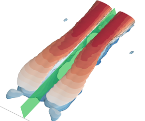
Figure 7. (a,c,e) Contours of  $u_{FM}$ superimposed with the associated in-plane velocity vectors at $y/h=0.5$. (b,d,f) The isosurfaces of $u_{FM}=-0.15\,|\hat {u}_{FM}|_{max}$ for the phase angles (a,b) $\alpha =-{\rm \pi} /6$, (c,d) $\alpha =0$ and (e,f) $\alpha ={\rm \pi} /9$, coloured by the vertical elevation ( $\kern0.7pt y/h$). An animated version of (a,c,e) is also provided as supplementary movie 3.
A conceptual vortex model evolving in 3-D space is proposed in figure 8 to incorporate all aforementioned kinematic and structural characteristics of FM, as well as those gleaned from the literature. When the low-velocity streak covers the separation bubble (as in figures 7a,b), the separated shear layer is elevated and flow reattachment is delayed. This accounts for the state of an enlarged separation bubble at a low frequency reported in the literature (e.g. Eaton & Johnston Reference Eaton and Johnston1982; Kiya & Sasaki Reference Kiya and Sasaki1983; Fang et al. Reference Fang, Tachie and Dow2022). This enlarged separation bubble in the  $x$–
$x$– $y$ plane, as shown in figures 8(a,b), is flanked by vertical (marked as VA) and streamwise (marked as SA) vortices in the first and second halves of the separation bubble, respectively, from a 3-D perspective. (Note that the mirrored versions of the vortices, such as VA $'$, are not explicitly commented on hereinafter for conciseness in the text.) The dominance of vertical vortices in the first half of the separation bubble has been shown in figure 6(b). The vertical vorticity ( $\omega '_2$) generated by $\partial u'/\partial z$ near the boundaries segregating the low- and high-velocity streaks in the spanwise direction is prone to stretching by positive $\partial V/\partial y$ (especially in the near-wall region around $x/h=4.0$; see figure 2b), and is therefore sustained in the first half of the separation bubble. The streamwise vortices in the second half of the separation, on the other hand, are stretched and sustained by the mean flow acceleration $\partial U/\partial x$ (see figure 2b), and their origin of generation is explained as follows.

Figure 8. A conceptual vortex model (not to scale) viewed from the (a,c,e) upstream and (b,d,f) side locations for the same phase angles as in figure 7. Notations VA , VB, SA, SB $'$ and so on are used to denote pertinent vortices. Here, the first letter (V or S) distinguishes the vertical and streamwise vortices, and the second letter (A or B) is for enumeration, whereas the superscript prime denotes a mirrored version. Note in (d) that vortex SA is further back into the viewing plane than vortices VB and SB, and vortex VA behind VB is omitted for clarity.
As the phase evolution continuous to that in figures 8(c,d) (or equivalently, figures 7c,d), the vortices VA and SA induce two interconnected pairs of opposite-signed vortices (marked as VB and SB). The vertical vortex VB is centred in the vicinity of  $x/h=4$ to be amplified by the local vertical stretching. The streamwise vortex SA, on the other hand, is near the crest of the separating streamline. The interconnection of the vertical vortex VB and streamwise vortex SB in figure 8(d) reflects a mutual induction mechanism and an absolute instability mechanism.
Let us elaborate this mutual induction mechanism first. Near the crest of the separating streamline, the mean shear  $\partial U/\partial y$ tilts streamwise vorticity to form vertical vorticity, and vice versa. This tilting effect is abrupt and creates a strong curvature at the crest of the separating streamline. The point where the vortices switch orientation is termed a ‘kink’, following Zhou et al. (Reference Zhou, Adrian, Balachandar and Kendall1999). Based on the discussion of the Biot–Savart law for hairpin structures by Zhou et al. (Reference Zhou, Adrian, Balachandar and Kendall1999), the strong curvature near the kink significantly enhances the velocity induction in the space flanked by counter-rotating vortices. Indeed, in the corner of VB and SB, the spanwise velocity $w'$ induced by SB can also drive VB, and vice versa, i.e. mutual induction. This mutual induction, along with the stretching by $\partial V/\partial y$ and $\partial U/\partial x$, strengthens VB and SB in the first and second halves of the separation bubble, respectively. Because of this process, the sweep event initiates near the crest of the separating streamline, and then spills over the entire separation bubble. Meanwhile, the low-velocity streak in the region above the separating streamline is altered only mildly. This, together with the sweep event underneath the separating streamline, weakens the instantaneous shear layer, while generating a ‘large vortex’. This ‘large vortex’ gradually deviates from its original position while decaying, and, in the process, introduces (albeit weak) disturbance outside the separation bubble. This ‘large vortex’ has been reported as a feature of FM (see also figure 6(a) here), and conjectured to be some irregularity of vortex shedding in the separated shear layer in the literature (e.g. Kiya & Sasaki Reference Kiya and Sasaki1983; Tafti & Vanka Reference Tafti and Vanka1991; Yang & Voke Reference Yang and Voke2001). With the above discussion, it is now clear that in fact this ‘large vortex’ is not due to the irregularity of vortex shedding, but is a consequence of abrupt switching between low- and high-velocity streaky structures due to the evolution of vortices initiated at the crest of the separating streamline.
Let us now comment on the instability mechanism sustaining FM. To this end, a negative  $v'$ near the crest of the separating streamline, as that induced by SB in figures 8(c,d), is considered. Since $V\approx 0$ for obvious reasons, an infinitesimal $u'$ is governed approximately by
 \begin{equation} \frac{\partial u'}{\partial t} + v'\,\frac{\partial U}{\partial y} + u'\, \frac{\partial U}{\partial x} +U\,\frac{\partial u'}{\partial x} \approx 0 . \end{equation}
Similar to the framework of Prandtl's mixing length hypothesis, the negative  $v'$ in the separated shear layer generates positive $u'$ (i.e. a sweep event, as marked in figure 8d), thus the second term of (3.4) is negative. With the negative $\partial U/\partial x$ near the crest of the separating streamline (see figure 2b), the third term of (3.4) is also negative. Because of the streamwise orientation of SB, $\partial u'/\partial x\approx 0$ holds, especially at the location of maximum $u'$, so that the fourth term of (3.4) is relatively negligible. It is therefore concluded that for the sweep event induced by SB near the crest of separating streamline, $\partial u'/\partial t$ is positive to further amplify the already-positive $u'$, i.e. instability. This instability is similar to the lift-up mechanism, which is described by (3.4) without the third and fourth terms as in Ellingsen & Palm (Reference Ellingsen and Palm1975). The third term of (3.4), due to the mean flow deceleration ( $\partial U/\partial x<0$) near the crest of separating streamline, provides an additional boost to the lift-up mechanism. This ‘boosted’ lift-up mechanism explains the elevated productions due to shear ( $Pr_{11,s}$) and deceleration ( $Pr_{11,n}$) for FM at the crest of the separating streamline (see figure 5c). This is also why the elevated levels of energy of FM (figure 4c) and the abrupt appearance of a sweep (or ejection) event (see the animation for figure 6a) are both near the crest of the separating streamline. This boosted lift-up mechanism is reminiscent of the absolute instability of streaky structures observed by Lanzerstorfer & Kuhlmann (Reference Lanzerstorfer and Kuhlmann2012a,Reference Lanzerstorfer and Kuhlmannb). This boosted lift-up mechanism cannot be captured by the instability analyses based on 1-D reverse-flow profiles (i.e. omitting the streamwise variation of base flow), which have demonstrated limited success in describing FM (e.g. Yang & Voke Reference Yang and Voke2001).
As the vortices VB and SB in figures 8(c,d) evolve to those in figures 8(e,f), the sweep event gradually covers the entire separation bubble, resulting in a high-velocity streak in the original location of the low-velocity streak. During this process, the vortex cores of VB and SB gradually deviate from the separated shear layer, so that the mutual induction becomes inactive. This breaks the connection between VB and SB to be as in figures 8(e,f). Subsequently, VB and SB in figures 8(e,f) act as opposite-signed versions of vortices VA and SA in figures 8(a,b), and this cycle repeats.
4. Conclusions
The fundamental mechanism of low-frequency flapping motion (FM) in flow separation is investigated using direct numerical simulation. In the mean flow reversal area, streamwise deceleration and acceleration (together with positive and negative  $\partial V/\partial y$, respectively) manifest in the first and second halves of the separation bubble, respectively. The separated shear layer, on the other hand, features not only the vertical shear (i.e. positive $\partial U/\partial y$) but also streamwise deceleration (i.e. negative $\partial U/\partial x$). Near the crest of the separating streamline, the lift-up mechanism due to shear is boosted by deceleration, and triggers the instability underlying FM. In the meantime, the shear abruptly tilts the streamwise vorticity to vertical vorticity (and vice versa), creating a strong curvature in the vortex filament. For this vortex filament, the vertical part is stretched by the positive $\partial V/\partial y$ in the first half of the separation bubble, and the streamwise part is stretched by the positive $\partial U/\partial x$ in the second half of the separation bubble. The vertical and streamwise parts of the vortex filament can also self-sustain by a mutual induction mechanism, and collaboratively create low-velocity (or high-velocity) streaky structures encompassing the entire separation bubble, so as to flap the separated shear layer up and down periodically. A ‘large vortex’ shedding manifests at the interface between the low- and high-velocity streaks during the sign switching, and introduces perturbation outside the separation bubble. This ‘large vortex’ is not the previously conjectured irregularity of vortex shedding residing in the separated shear layer in the literature. Overall, FM is unstable, self-sustained, and manifests outside the separation bubble, and therefore represents an absolute (global) instability.
The frequency  $f$ of FM, when scaled by the mean reattachment length $L_r$ and free-stream velocity $U_\infty$, is well known to be within a narrow band $St_{Lr}\equiv f\kern0.5pt L_r/U_\infty \in [0.08,0.20]$, regardless of geometry, pressure gradient or Reynolds number. This hints at the universality of FM. As has been elucidated, FM is triggered by a boosted lift-up mechanism at the crest of the separating streamline, which relies on the co-existence of shear (positive $\partial U/\partial y$) and deceleration (negative $\partial U/\partial x$). This co-existence of shear and deceleration is expected to be universal for separated shear layers since they are always convex. The evolution of FM also involves the positive $\partial V/\partial y$ (equivalently, negative $\partial U/\partial x$) and positive $\partial U/\partial x$ in the first and second halves of the separation bubble, respectively. The negative and positive values of $\partial U/\partial x$ are separated naturally in space by the maximum reverse flow at the centre of any separation bubbles. The topological distribution of these mean (or base) flow properties supporting FM is thus universal, and the mean reattachment length $L_r$ is indeed an appropriate length scale for FM. Therefore, the universality of FM is suggested.
Supplementary movies
Supplementary movies are available at https://doi.org/10.1017/jfm.2024.280.
Acknowledgements
X.F. is indebted to Professor M.F. Tachie for the countless stimulating discussions on flapping motion over the years. The inspiring suggestions provided by anonymous reviewers are also gratefully acknowledged.
Funding
This work was supported by the National Key R&D Program of China (2021YFA0719200) and the National Natural Science Foundation of China (12325207).
Declaration of interests
The authors report no conflict of interest.


