


1. Introduction
The term cavitation refers to the rapid phase change of liquid when the pressure is decreased below a critical level. It has been of interest in great part because of the noise that it generates as well as the destructive effect that it has on the performance and life of turbomachines and hydraulic structures (Arndt Reference Arndt1981; Brennen Reference Brennen2014). Hydrodynamic cavitation can appear as attached cavitation on curved surfaces (Arakeri & Acosta Reference Arakeri and Acosta1973; De Chizelle, Ceccio & Brennen Reference De Chizelle, Ceccio and Brennen1995) or in the core vortices within e.g. jets, separated flows and wakes (Arndt Reference Arndt2002). Cavitation is often parameterized using the cavitation index,  $\sigma = 2(P - {P_v})/\rho {U^2}$, where P is a reference pressure, Pv the vapor pressure of water, ρ the water density and U a reference velocity. The index corresponding to the pressure at cavitation inception is referred to as σi. Prediction of cavitation inception in turbulent flows has remained a challenge since the process involves interactions of the unsteady pressure fields with nucleation sites, both of which are stochastic in nature. Hence, while there have been many attempts to develop semi-empirical relations for cavitation inception in vortices, e.g. by McCormick (Reference McCormick1962) for tip vortices, subsequent studies have shown substantial differences from measured data (Arndt & Keller Reference Arndt and Keller1992; Shen, Gowing & Jessup Reference Shen, Gowing and Jessup2009). In general, the cavitation inception index in turbulent flows varies with the geometry involved, Reynolds numbers, turbulence level, dissolved gas content and free-stream nuclei distribution. In some cases, σi is sensitive to subtle changes to the flow structure. For example, in the near field of jets σi generally increases with scale (Ooi Reference Ooi1985; Gopalan, Katz & Knio Reference Gopalan, Katz and Knio1999), but tripping of the boundary layer upstream in the nozzle lowers σi significantly as the preferred sites of cavitation inception changes from secondary vortices to the primary vortex rings. In shear layers, compilation of data from several measurements shows that the cavitation inception index increases with Reynolds numbers (Katz & O'Hern Reference Katz and O'Hern1986; O'Hern Reference O'Hern1990). The reasons for this trend have not been explained, and are in contrast with scaling of flow structures associated with Kelvin–Helmholtz instabilities (Brown & Roshko Reference Brown and Roshko2012). For tip vortices, the observed Reynolds number effects on σi appear to become more pronounced with decreasing non-condensable dissolved gas content, therefore Arndt, Arakeri & Higuchi (Reference Arndt, Arakeri and Higuchi1991) attribute it to effects of nuclei, whose characteristics do not scale with the velocity squared.
In the near field of a turbulent shear layer, cavities appear first in the core of quasi-streamwise vortices (QSVs) developing between the primary spanwise structures with their lengths being over five times larger than their diameters (Katz & O'Hern Reference Katz and O'Hern1986). Numerous studies have described the formation and strength of these quasi-streamwise structures (e.g. Jimenez Reference Jimenez1983; Bernal & Roshko Reference Bernal and Roshko1986; Lasheras & Choi Reference Lasheras and Choi1988; Bell & Mehta Reference Bell and Mehta1992). They are intermittent, often occurring as counter-rotating pairs, and have a strength that is 10 %–40 % of those of the primary spanwise vortices. However, there is no information about the pressure in their cores and their relation to the primary flow parameters, which is essential for understanding cavitation inception. In various settings, cavitation in secondary vortices appear as elongated strings, with their lengths being over five times larger than their diameters (Katz & O'Hern Reference Katz and O'Hern1986; Gopalan et al. Reference Gopalan, Katz and Knio1999; Moisy, Voth & Bodenschatz Reference Moisy, Voth and Bodenschatz2000; Chang et al. Reference Chang, Choi, Yakushiji and Ceccio2012; Barbaca et al. Reference Barbaca, Venning, Russell, Russell, Pearce and Brandner2020). It has been argued (Gopalan et al. Reference Gopalan, Katz and Knio1999; Chang et al. Reference Chang, Choi, Yakushiji and Ceccio2012) that the low pressure inside the secondary vortices develops owing to their stretching by the primary structures. In the near field of jets, Gopalan et al. (Reference Gopalan, Katz and Knio1999) show that the estimate rates of cavitation events based on the measured nuclei distribution and statistics of straining of vortices are consistent with the observed rates, i.e. they have the same order of magnitude. However, their calculated trends with cavitation number differ from the observed ones. For a pair of parallel tip vortices with different strength, Chang et al. (Reference Chang, Choi, Yakushiji and Ceccio2012) estimate the pressure minima in the vortex core based on the measured nuclei sizes, cavitation inception indices, initial cross-sectional velocity distribution and estimated straining history. They conclude that reduction in the vortex core diameter owing to axial straining alone is not sufficient for explaining the measured cavitation inception indices, and attribute the discrepancy to the axial velocity and acceleration in the vortex core. They also argue that observed asymmetry in the growth rate of the cavity along the vortex core is indicative of axial variations in velocity and acceleration.
Several studies have discussed the axial variations along cavitating tip vortices (e.g. Arndt et al. Reference Arndt, Arakeri and Higuchi1991; Green & Acosta Reference Green and Acosta1991). Arndt et al. (Reference Arndt, Arakeri and Higuchi1991) state that the inherent axial pressure gradients in tip vortices (Batchelor Reference Batchelor1964) results in localized inception of cavitation in the vortex core. Barbaca et al. (Reference Barbaca, Venning, Russell, Russell, Pearce and Brandner2020) note that, as the cavitating strings collapse, they leave behind several remnants along the vortex axis. Moisy et al. (Reference Moisy, Voth and Bodenschatz2000) observe that cavitation inception in vortex filaments located in a turbulent flow between two counter-rotating disks can occur in multiple discrete points along the vortex axis. They refer to this phenomenon as ‘necklace’ cavitation. With further decrease in pressure, as the cavitating structures become continuous long strings, they develop helical undulations, which have been studied in the context of tip vortices e.g. by Crow (Reference Crow1970) and Widnall (Reference Widnall1975). Based on numerical simulations (Lundgren & Ashurst Reference Lundgren and Ashurst1989; Melander & Hussain Reference Melander and Hussain1994; Verzicco, Jiménez & Orlandi Reference Verzicco, Jiménez and Orlandi1995), these undulations have been attributed to the dynamics of axially strained vortices. The resulting axial pressure gradients generate waves along the vortex axis, a topic discussed extensively in the literature starting with the inviscid analysis by Kelvin (Reference Kelvin1880). Based on the direct numerical simulations (DNS) by Verzicco et al. (Reference Verzicco, Jiménez and Orlandi1995), the time evolution of the vortex structure and its stability depend on the strain rate, viscosity (Reynolds number) and vortex strength. Depending on their relative contributions, the axial waves can stabilize the vortex, homogenizing its core size, or sustain the core radius oscillations, or promote the vortex diffusion owing to viscous effects. Hence, the stability of the vortex depends on the Reynolds number. For time-dependent strain fields, Verzicco & Jimenez (Reference Verzicco and Jimenez1999) show that if the period of oscillatory straining is smaller than the time required for the vortex to balance the axial strain by pressure gradients, the strength of this vortex decays. For longer periods, the vortex may maintain its strength for a long time. To the best of our knowledge, experimental data on axial pressure gradients in stretched vortices are not available from any source.
Cavitation inception occurs when nuclei, mostly microbubbles, are exposed to a pressure falling below a bubble size-dependent critical level. The pressure gradient field also affects the entrainment of bubbles into vortices (Sene, Hunt & Thomas Reference Sene, Hunt and Thomas1994; Sridhar & Katz Reference Sridhar and Katz1995; Spelt & Biesheuvel Reference Spelt and Biesheuvel1997). Nuclei availability, dynamics and effects on cavitation inception have been investigated extensively (e.g. Billet Reference Billet1985; Arndt & Keller Reference Arndt and Keller1992; Khoo et al. Reference Khoo, Venning, Pearce, Takahashi, Mori and Brandner2020). Most water tunnels and environmental water contain microbubbles typically ranging in size from microns to millimetres. The nuclei content depends on the tunnel operating conditions, including dissolved gas content, pressure time history and circulation time (Liu, Sato & Brennen Reference Liu, Sato and Brennen1993). Studies of cavitation inception require control and characterization of the nuclei content, as recent studies have begun to achieve (Khoo et al. Reference Khoo, Venning, Pearce, Takahashi, Mori and Brandner2020). Since this task is often quite difficult, many prior studies have used instead means of assessing the susceptibility of the water to cavitation inception (Oldenziel Reference Oldenziel1982; d'Agostino & Acosta Reference d'Agostino and Acosta1991). Once cavitation starts, remnants of collapsing cavities become nucleation sites for new cavitation events (Barbaca et al. Reference Barbaca, Venning, Russell, Russell, Pearce and Brandner2020; Ram, Agarwal & Katz Reference Ram, Agarwal and Katz2020), increasing their frequency. The lifetime of cavitating structures is typically a few milliseconds, i.e. comparable to the time scales of the larger flow structures like that of the disk motion for Moisy et al. (Reference Moisy, Voth and Bodenschatz2000) or of the vortex motion in a shear layer in Barbaca et al. (Reference Barbaca, Venning, Russell, Russell, Pearce and Brandner2020). This lifetime is substantially longer than the duration of the initial explosive growth or the final collapse, which typically take place in less than a millisecond (Ran & Katz Reference Ran and Katz1994; Choi et al. Reference Choi, Hsiao, Chahine and Ceccio2009).
Inherently, the number, spatial distribution and duration of pressure minima in turbulent flows affect the likelihood or rate of cavitation inception events. While considerable effort has already been invested in attempts to characterize the interactions of nuclei with the pressure field (Brennen Reference Brennen2014), until recently, the research community have not had the means of determining the pressure field in turbulent flows away from boundaries. Hence, numerical simulations have been the primary source of information on the pressure in the core of eddies, although limited in Reynolds numbers. Recent studies aimed at understanding inception using Lagrangian pressure statistics following fluid elements or micro-bubbles have been performed for isotropic turbulence based on DNS data (Bappy, Carrica & Buscaglia Reference Bappy, Carrica and Buscaglia2019; Bappy et al. Reference Bappy, Carrica, Vela-Martín, Freire and Buscaglia2020). They show that pressure minima appear more frequently and have increasing durations with increasing Reynolds number. Furthermore, Bappy et al. (Reference Bappy, Carrica, Vela-Martín, Freire and Buscaglia2020) also show that the trapping of bubbles by vortices, hence exposure to low pressure events, increases with nucleus size. Their pressure probability density functions (PDFs) have significant negative tails, that increase with Reynolds number. This is not always the case for turbulent shear layers. Wall pressure fluctuation measurements by Lee & Sung (Reference Lee and Sung2001) behind a backward-facing step exhibit a nearly Gaussian behaviour, in agreement with recent results of large eddy simulations by Brandao & Mahesh (Reference Brandao and Mahesh2022), at least for non-cavitating flows. However, negative tails appear once cavitation starts.
Turbulent pressure fluctuations away from boundaries have been challenging to measure. Experiments involving transducers inserted in the flow field have a broad frequency range but have a limited spatial resolution and are inherently intrusive (George, Beuther & Arndt Reference George, Beuther and Arndt1984; Tsuji & Ishihara Reference Tsuji and Ishihara2003). To alleviate the issue of intrusion, Ooi & Acosta (Reference Ooi and Acosta1984) introduce the use of microbubbles as pressure sensors. Following calibrations tests (Ran & Katz Reference Ran and Katz1991), Ran & Katz (Reference Ran and Katz1994) have used this method the characterize the pressure in the near field of a jet. Since then, there have been significant advances in calculating the pressure from time-resolved particle image velocimetry (PIV) data, too many to summarize in a short introduction. To obtain the pressure, most applications either use integration of material acceleration (Liu & Katz Reference Liu and Katz2006, Reference Liu and Katz2013; Dabiri et al. Reference Dabiri, Bose, Gemmell, Colin and Costello2014; Wang, Zhang & Katz Reference Wang, Zhang and Katz2019) or solve the pressure Poisson equation (van Oudheusden et al. Reference van Oudheusden, Scarano, Roosenboom, Casimiri and Souverein2007; Ghaemi, Ragni & Scarano Reference Ghaemi, Ragni and Scarano2012; Villegas & Diez Reference Villegas and Diez2014), as summarized in several recent comparative papers (Charonko et al. Reference Charonko, King, Smith and Vlachos2010; van Gent et al. Reference van Gent, Michaelis, van Oudheusden, Weiss, de Kat, Laskari and Schrijer2017; Liu & Moreto Reference Liu and Moreto2020). Early applications have been based on planar data assuming two-dimensional (2-D) flows, but in recent years, with the introduction of 3-D tomographic PIV (Elsinga et al. Reference Elsinga, Scarano, Wieneke and Van Oudheusden2006; Schanz, Gesemann & Schröder Reference Schanz, Gesemann and Schröder2016), the measurements are based on 3-D integrations. Several techniques have been developed to improve the uncertainty in pressure. For example, uniformly distributed omni-directional integration of pressure gradients has been introduced to minimize the adverse effects of error propagation (Liu & Katz Reference Liu and Katz2006; Wang et al. Reference Wang, Zhang and Katz2019; Liu & Moreto Reference Liu and Moreto2020). Data assimilation techniques that utilize known physics to augment the measured data have also been developed. Among them, the vortex-in-cell method, minimizes the difference between the measured velocity and material acceleration from predictions based on the vorticity transport equation (Schneiders & Scarano Reference Schneiders and Scarano2016). Another approach involves a constraint cost minimization procedure that forces the velocity field to be divergence free and the material acceleration curl free (Agarwal et al. Reference Agarwal, Ram, Wang, Lu and Katz2021). Effects of other contributors, e.g. viscous diffusion especially near boundaries, data resolution and experimental errors, have also been evaluated (Azijli et al. 2016; Jeon et al. 2018; Agarwal et al. Reference Agarwal, Ram, Wang, Lu and Katz2021). These techniques have recently been implemented to measure the pressure in a variety of turbulent flows, such as a boundary layer by Ghaemi & Scarano (2013), boundary layer over compliant surface by Zhang et al. (2017) and flow over a serrated trailing edge by Lima Pereira et al. (Reference Lima Pereira, Ragni, Avallone and Scarano2020). In the present paper, we use these techniques for understanding the impact of the pressure field on the cavitation inception in a turbulent shear layer developing behind a backward-facing step.
The flow and turbulence behind a downstream-facing step has been studied extensively, starting from the experimental work by Eaton & Johnston (Reference Eaton and Johnston1982) and the DNS by Le, Moin & Kim (Reference Le, Moin and Kim1997). In addition to the free shear layer, this flow includes a recirculation region under the shear layer and a reattachment zone where the shear layer attaches to the wall. Fluctuations in the size of the separated bubble cause low-frequency flapping of the shear layer and location of the reattachment point (Driver, Seegmiller & Marvin Reference Driver, Seegmiller and Marvin1987; Wee et al. Reference Wee, Yi, Annaswamy and Ghoniem2004). Most of the pressure measurements for the flow behind a backward-facing step have been performed using sensors attached to the wall, e.g. Lee & Sung (Reference Lee and Sung2001). Considering that cavitation inception occurs in the secondary structures away from the boundary, these measurements have limited relevance to cavitation inception. Yet, they show that the wall pressure fluctuations rise rapidly at 50 % of flow reattachment length, owing to the influence of the primary spanwise vortices. These vortices are convected at two different velocities, the first larger than 60 % of the free-stream velocity (U) and the second ranging between 0.2U and 0.4U. The former speed corresponds to a ‘shear layer’ mode, where the vortices grow as they are advected downstream, and the latter to a ‘wake’ mode, where the shear layer and vortices expand suddenly while lingering, and then accelerate. The presence of these modes has been deduced based on wall pressure measurement for non-cavitating flows by Hudy, Naguib & Humphreys (Reference Hudy, Naguib and Humphreys2007) as well as for developed cavitating flows by Maurice et al. (Reference Maurice, Machicoane, Barre and Djeridi2021). For the latter case, transition to the wake mode is favoured. The structure of developed cavitation and compressible flow phenomena are investigated based on wall pressure measurements and X-ray densitometry by Bhatt, Ganesh & Ceccio (Reference Bhatt, Ganesh and Ceccio2021).
Understanding the causes for trends with Reynolds numbers as well as appearance of inception requires characterization of both the pressure field generated by the secondary QSVs, and the entrainment of nuclei into them. To determine the effects of strain field on the pressure, simultaneous 3-D flow and pressure measurements as well as statistical analyses in Eulerian and Lagrangian reference frame are necessary. These analyses elucidate the mechanisms affecting the time evolution of pressure and the observed occurrence of multiple cavitation inception events along the same QSV. Trends are explained in the context of a stretched vortex dynamics. The effect of nuclei on cavitation inception is studied based on the trajectories, spatial distribution and concentration of bubbles within and outside of the shear layer under controlled and ‘natural’ nuclei seeding. The set-up and techniques are described in the next section. They are followed by the results, statistical analysis and discussion in § 3, and by conclusions in § 4.
2. Methods
2.1. Experimental set-up
Facility: the experiments have been performed in a small water tunnel powered by two centrifugal pumps located 5 m below the test section, as described in Gopalan & Katz (Reference Gopalan and Katz2000) and Ling et al. (Reference Ling, Srinivasan, Golovin, Mckinley, Tuteja and Katz2016). This tunnel is equipped with a 1000 litre buffer tank located between the pumps and the test section in order to remove free-stream bubbles, followed by a settling chamber containing a honeycomb and meshes and a smooth 9:1 area contraction leading to the test section. The 405 × 63 × 51 mm3 test section is fitted with a backward-facing step to generate a free shear layer, as illustrated in figure 1(a). The step height h is 10 mm, resulting in an expansion ratio, namely height of the test section after the step relative to that before the step, of 1.19. The shape of the curved surface upstream of the step is a fifth-order polynomial to ensure that the curvature is nearly zero at both ends to prevent undesirable pressure gradients there. The curved surface is followed by a 25 mm long flat horizontal section that terminates at the step. To trip the boundary layer, V-shaped grooves are machined in the bottom wall near the entrance to the test section, 159 mm upstream of the step (figure 1b). These grooves are similar to those described in Ling et al. (Reference Ling, Katz, Fu and Hultmark2017), where it is shown that the mean velocity profile 230 mm downstream of the grooves is consistent with that of a fully developed turbulent boundary layers, with viscous, buffer, log and outer layers. Taps located at the inlet to the test section are used for measurements of the reference pressure and dissolved gas content, and for injection of controlled free-stream nuclei. The pressure is measured using a Setra model 230 differential pressure transducer, and the dissolved oxygen content is measured using an optical fibre sensor, FireStingO2 manufactured by PyroScience. The mean pressure above the step, used to calculate the cavitation indices, is inferred from the measured pressure using Bernoulli's equation.

Figure 1. The experimental set-up: (a) a spanwise view of the test section with a backward-facing step. The two fields of view (FOVs) of the two-dimensional PIV measurements are marked in green (solid and dot-dash); the FOV for backlit cavitation imaging is marked in blue; and the tomographic PIV and holographic cavitation imaging areas are marked in red. (b) A magnified view of the inlet to the test-section with a tap for bubble injection and the V-shaped tripping grooves. (c) The bubble injector showing a couple of 60 μm diameter bubbles. A magnified view of a train of injected microbubbles along the bottom wall can also be seen in (a).
Measuring the mean flow profiles: several experiments have been performed to characterize the non-cavitating flow as well as the conditions for cavitation inception within the fields of views marked in figure 1(a). Two-dimensional PIV has been used for characterizing the mean flow and Reynolds stresses for mean free-stream velocities above the step of U = 1.45, 5.3, 10.5 and 16 m s−1 in an area extending from the separating boundary layer all the way to the reattachment region. To cover this area while maintaining an acceptable resolution, the 2-D PIV images are recorded in a pair of slightly overlapping 36.3 × 24.2 mm (x × y) sample areas using a 6600 × 4400 pixel interline transfer CCD camera, Imperx Model BB640. The thin light sheet that illuminates the spanwise-centred plane is generated using a Quantel Evergreen Nd:YAG laser, and the flow is seeded with 2 μm silver-coated glass particles (Conduct-o-Fil SG02S40, specific gravity of 3.5). The time delay between image pairs is adjusted to maintain a 90 μm displacement between exposures in the free stream. Cross-correlation analysis is performed using the LaVision DaVis® 10 software package. Using multi-pass correlations with the final interrogation area being 32 × 32 pixels, and 75 % overlap between windows, the resulting velocity vectors spacing is 43 μm. Approximately 2000 realizations are used to obtain the mean flow and the Reynolds stress statistics for each speed. The typical uncertainty in instantaneous velocity, corresponding to 0.1–0.2 pixels, is 1 %. Ensemble averaging should reduce this uncertainty by more than an order of magnitude.
Locating cavitation inception: in experiments without seeding of the flow with bubbles (and particles), which are referred to as ‘natural’ nuclei, the appearance including the size, location and durations of the cavitation events have been characterized at U = 10.5 and 16 m s−1 using two synchronized orthogonal views. For the range of pressures that could be maintained steadily in the tunnel, we cannot examine cavitation below 7 m s−1. The side and top views are recorded for 2.55 s at 3932 Hz at the resolution of 30 μm with PCO.dimax S4 high speed digital cameras. The 52 × 21 mm field of view is marked in figure 1(a) in blue. Two halogen lamps are used for back lighting the test section, enabling an exposure time of 4 μs. During image acquisition, the pressure in the tunnel is maintained at a constant level corresponding to σ varying between 0.45 and 0.55. The water is de-aerated by running the facility at a low pressure before the experiment. The pressure is then raised to well above the desired conditions, and then lowered just before the experiment to minimize the concentration of free-stream bubbles. In this way, the dissolved oxygen content in the water is kept close to 70 % of the saturation level based on the pressure at the inlet to the test section. The concentration and size distribution of free-stream bubbles are monitored throughout the experiments using the procedures described below.
Generation of bubbles: the entrainment of nuclei and their effects on cavitation inception are studied under controlled injection of microbubbles. In this case, the water is de-aerated to less than 50 % of the saturation levels of dissolved oxygen at an inlet pressure of 1.1 bar. The flow is then seeded with a train of 60 μm diameter bubbles using a bubble generator designed based on the procedures described by Toshiyuki Matsumi et al. (Reference Toshiyuki Matsumi, José da Silva, Kurt Schneider, Miguel Maia, Morales and Araújo Filho2018) and shown in figure 1(c). It consists of a 3D printed T-junction with an ORIGIO MIC-SLM-30 micropipette with an exit diameter of 4.3–4.9 μm connected to a compressed source of nitrogen. The injected air is sheared by a parallel stream of water introduced through the second inlet to generate a monodisperse bubble train with size and injection frequency that vary with the pressures of the two fluids. The 60 μm diameter bubble train is generated using gas pressure varying between 2 and 3 bar and water pressure of 1.2 bar. Pressure controllers and transducers with accuracy of 0.001 bar are installed to maintain the pressure in the incoming water and air streams. The gas pressure is adjusted to maintain a distance of 0.3–0.4 mm between bubbles as they are introduced into the water tunnel, namely the separation between bubbles is approximately 5 to 7 times the diameter. Hence, the bubble generation rate increases with velocity. As a reference, the rate is 3000 Hz at U = 1 m s−1. This procedure has resulted in bubble concentration of about 0.06 mm−3 in the free stream above the shear layer for all speeds, as described in § 3.4. The speed of the liquid jet injected into the tunnel is 0.35 m s−1, and the site of injection from the wall is located near the inlet, just upstream of the tripping elements (figure 1b). Given this low speed of injection and its location upstream of the trips, we presume that the injection has little effect on the flow. Furthermore, owing to the small bubble size, and consistent with images recorded at the exit from the injector, the bubbles do not deform noticeably. Finally, the buoyant rise velocity of these bubbles assuming Stokes flow, 1.8 mm s−1 (Clift, Grace & Weber Reference Clift, Grace and Weber2005), is three orders of magnitude lower than the free stream. Assuming that the bubbles are advected at the free-stream velocity, the buoyant rise of these bubbles between the injection point and the step is 0.2 mm at 1.45 m s−1, and even lower at the higher speeds. Between different experiments, the tunnel is pressurized for a few minutes to minimize the concentration of bubbles not originating from the injection system in the free stream, the shear layer and the recirculation zone. Yet, reference data for the free-stream bubble distribution away from the shear layer are also quantified.
Detecting cavitation inception: focusing on regions of high cavitation, microscopic cinematic inline holography (Sheng, Malkiel & Katz Reference Sheng, Malkiel and Katz2006; Katz & Sheng Reference Katz and Sheng2010) has been used to capture the growth and collapse of cavitation events. This method can be used for determining the size, shape and 3-D location of bubbles, albeit at a coarser resolution in the axial direction of the illuminating laser beam. To resolve the bubble growth during cavitation inception, the camera should have an acquisition rate exceeding 100 000 frames per second. Hence, a Kirana model 5M camera, with image size of 924 × 768 pixels and maximum frame rate of 5 × 10⁶ s−1 is used for recording spanwise-aligned holograms. However, since this camera can only record 180 frames, it must be triggered by a fast event detector. We opt to use the image of the perpendicular top-view camera, a Phantom model v2640 CMOS camera, which operates at 50 kHz, for triggering the Kirana. This triggering is based on detection of intensity changes in a selected part (200 × 100 pixels) of the hologram captured by the Phantom camera. The Kirana's resolution is 7 μm pixel−1, and the images are recorded at 200–300 kHz, while the Phantom camera operates at a magnification of 12.5 μm per pixel. As illustrated in figure 2(b), the perpendicular holography systems use the same light source, a collimated beam generated by a pulsed Katana-05-HP green (532 nm) laser manufactured by NKT Photonics that has a pulse duration of 0.8 ns and generates 4 μJ pulse−1. This laser operates continuously at 1 MHz, and both cameras use their internal electronic shutter system to acquire single exposures in each frame. For the experiments, the pressure in the tunnel is lowered until an event is detected by the Phantom camera. This also triggers recording of the tunnel inlet pressure, which results in σ ranging from 0.45 to 0.55.

Figure 2. Optical set-up: (a) top view of the tomographic PIV system consisting of four cameras with lenses aligned perpendicularly to acrylic prisms. The sample area illuminated by a thick laser sheet is shown in green. (b) A downstream view showing the two-view holography set-up.
Tracking of bubbles: the perpendicular hologram set-up has also been used to record the bubble population over the entire shear layer span and in the free stream above the shear layer under non-cavitating conditions. In this case, the holograms are acquired at nearly the same resolution of 12.5 μm per pixel, which allows characterization of bubble size and concentration when their size exceeds 50 μm. For tracking of bubbles, both cameras acquire images at 8, 50 and 62 kHz for free-stream velocities of 1.45, 10.5 and 16 m s−1, respectively. Data have been acquired while keeping the facility at a constant pressure of 1.1 bar, which results in σ of 106, 1.75 and 0.6 at 1.45, 10.5 and 16 m s−1, respectively.
Three-dimensional velocity and pressure measurements: time-resolved tomographic PIV (figure 2a) measurements have been performed to study the structure of secondary vortices (QSVs) and the pressure within them. Unfortunately, our tomographic PIV system can acquire data at a maximum framerate of 15 kHz, hence the 3-D time-resolved measurements needed for pressure calculations could only be performed at U = 1.45 and 5.3 m s−1. At 15 kHz, the displacement between exposures at 10.5 and 16 m s−1 are 0.7 and 1.07 mm, respectively, too large for resolving secondary vortices with characteristic size of ~1 mm. Therefore, at 5.3 m s−1 the data are recorded at 14 925 Hz with an image size of 624 × 380 pixels (maximum possible), resulting in a displacement of 355 μm between exposures. At 1.45 m s−1, the 1008 × 596 pixel images are recorded at 7407 Hz, giving a displacement of 196 μm. Thus, the normalized temporal resolution is almost twice at the lower speed, being 0.02h/U at 1.45 m s−1 and 0.035h/U at 5.3 m s−1. In both frame rates, the image sizes correspond to the maximum capabilities of the cameras. The 12.5 × 7.5 × 4.5 mm3 field of view extends horizontally from x = 0.5xr to 0.7xr, from y = −0.6h to 0.1h and from z = −0.2h to 0.2h (z = 0 is the spanwise centreline). The optical set-up involves four PCO.dimax S4 CMOS cameras with Nikon 105 mm lens arranged in the same plane (figure 2a), that is they are rotated only along the wall-normal axis at angles of ±15° and ±40° with the spanwise direction. Acrylic prisms are placed in front of each lens to reduce the effect of mis-matched refractive index at the walls and Scheimpflug adapters are used to rotate the cameras relative to the lens to keep the sample volume in focus. The light source is Photonics DM60-527 Nd:YLF laser whose beam is allowed to expand and then masked to generate a 4.5 mm wide slab in the sample area. The flow is seeded with 13 μm diameter silver-coated hollow glass spheres (Conduct-o-Fil SH400S20) that have a specific gravity of 1.6, leading to a characteristic time for the particles of 14 μs. The entire recording time is 2 s, i.e. 300h/U for 1.45 m s−1 and 1020h/U for 5.3 m s−1, during which the pressure at the entrance to the test section is held constant. The raw data that have been analysed consist of 28 000 and 15 000 realizations at 5.3 and 1.45 m s−1, respectively. This large database allows for evaluating the time evolution of different flow quantities, such as pressure, vorticity, etc.
2.2. Data analysis
Analysis of cavitation images and nuclei distribution: the data recorded using ‘natural’ seeding have been used for determining the location of cavitation inception, the void fraction, as well as the spatial and size distribution of bubbles in various locations within and outside of the shear layer during the early phase of cavitation. Cavitation events are defined by first segmenting the images using Otsu's method, which allows for adaptive thresholds (Otsu Reference Otsu1979). The resulting structures are described using an ellipse that has the same second central moments. Then, the diameter of the structure is the minor axis length of the ellipse and the length is the major axis length. Structures with eccentricity over 0.866, that is length over twice the diameter, and equivalent diameter (geometric mean of length and diameter) over 0.3 mm, whose centroid move with speeds between 10 % and 90 % of the free-stream velocity are selected as cavitation events. The thresholds for size and aspect ratio have been selected based on visual inspection. Selecting a fraction of the data, the analysis has been performed using eccentricity thresholds 0.866, 0.85, which is close to the chosen level, and 0.916, which is far from it. The results show that the F1 scores, which are the harmonic mean of the precision and recall of a classifier (Van Rijsbergen Reference Van Rijsbergen1979), are 0.89, 0.9 and 0.71 for thresholds of 0.85, 0.866 and 0.91, respectively. Restricting the speed range helps in cavity tracking, and reduces the likelihood of identifying noise as cavities. The analysis is performed using a single side view over the entire shear layer over nearly the entire span. The void fraction at each pixel is calculated based on the sum of diameters of the structures at the time when cavitation is detected normalized by the depth of the volume and the time of recording. The results have subsequently been used for selecting the location of pressure measurements. Using both side and top views, orientation of the cavities in x–y and x–z planes are detected. The orientation is the direction of the eigenvector associated with the largest eigenvalue of the second central moments. Then, the 3-D orientation of the cavity is calculated by matching the two projections. The distributions of smaller bubbles in the cavitating shear layer, free stream and recirculation region are also determined using the data recorded in the two perpendicular directions. For each, the sample volume size is 2 × 2 × 20 mm3, and their locations are marked in figure 28(a). These bubbles are also constrained to have an eccentricity of less than 0.86 and equivalent diameters between 0.1 and 1.3 mm to eliminate detection of cavitating structures. The analysis is based on the side view, and the top view is used for determining the spanwise locations of nuclei. Only bubbles detected by both cameras are counted.
Holograms with controlled seeding of microbubbles are recorded at fine spatial and temporal resolution, thus allowing for characterizing the size and growth rate of cavitation inception events as well as the distances between neighbouring events. For this analysis, 95 sets of 1200 time-resolved top-view holograms are reconstructed in planes separated by 150 μm in depth (Katz & Sheng Reference Katz and Sheng2010). The reconstructed planes are then added together to obtain a ‘compressed’ image of all the objects in the sample volume. The location of the cavities and their size are determined by thresholding this image, and finding contiguous objects using the MATLAB® functions bwconncomp and regionprops. Structures with a minimum size of 0.15 mm are selected as cavitation events but only if they are detected in several frames, and the velocity of their centroid is lower than the free-stream velocity. The location of these structures in the y direction is determined from the original reconstructed holograms by finding the focus depth using the minimum intensity and edge sharpness based on Tenengrad maps, following Gao et al. (Reference Gao, Guildenbecher, Reu and Chen2013). Based on manual evaluation of samples, using the perpendicular-view data, the depth uncertainty is approximately 180 μm. This procedure provides the 3-D location of the centroids of the cavities, their size (cross-section) and the rate at which this size changes in time. For both speeds, around 5200 cavities are tracked in time. To determine the orientation of vortices in which the cavities are located, especially when the cavities are nearly spherical, we rely on the fact that multiple cavities form along the same vortex. To define the vortex orientation, the detected cavities are expanded in all directions by 0.25 mm while retaining their shape. Linked blobs are considered to be parts of the same vortex if they are aligned in the same direction (within 15°). For original cavities with spherical shape, the vortex alignment is defined by linking it to its nearest blob and finding the orientation of the joined blob.
The concentrations and evolution of nuclei in the case of bubble injection are also quantified in the shear layer and in the free stream. The free-stream data are obtained by analysing the holograms recorded by Phantom camera, focusing on a volume extending from 2 to 20 mm above the step. The shear layer nuclei distributions are obtained by analysing the holograms recorded by the Kirana camera, focusing on an 18 mm deep sample volume located offset 3 mm from the spanwise centre of the test section (−0.6 < z/h < 1.2). First the holograms are spatially band-pass filtered in the frequency domain at wavenumbers corresponding to wavelengths of 30 μm (2.5 pixels) and 400 μm to remove undesired noise. The filtered holograms are reconstructed in planes separated by 25 μm in depth. The depth of the nuclei, that is the location along the wall-normal direction, is calculated based on the procedure involving Tenengrad maps described above and in Gao et al. (Reference Gao, Guildenbecher, Reu and Chen2013). The minimum intensities over slabs with 0.75 mm depth are then compressed to planar images, reducing the 3-D data to 12 slabs. The location and size of bubbles in each slab are determined using a random forest algorithm (Ho Reference Ho1995). The pixel classification module in ilastik, an interactive machine learning software (Berg et al. Reference Berg2019), is used to train a model that distinguishes between in focus bubbles and background. Lu et al. (Reference Lu, Ram, Jose, Agarwal and Katz2021) describe a similar procedure to find size distributions of free-stream bubbles in a water tunnel. Since some of the images still give false positives (noise detected as bubbles), the probability maps subsequently are compressed over the entire depth to a single plane, and sequences of 20 successive time steps are used for training a second model. This model detects bubbles that appear in more than a single frame and move in at least some of the images, i.e. they are not stationary. The resulting probability maps are then binarized and tracks are built based on displacements of the resulting sparse bubbles in successive frames. To validate the measurements and assure that perpendicular views give compatible results, a set of 40 top-view holograms are processed at depths corresponding to the shear layer. Results are then compared with those observed in the perpendicular view, showing that 92 % of the detected bubbles appear in both views, and that their sizes differ by 0.5 %, representing our uncertainty in bubble size. Data derived from over 3000 holograms in the free stream and 2700 in the shear layer, resulting in 40 000–90 000 nuclei for U = 1.45, 10.5 and 16 m s−1 each, are presented in this paper.
Velocity and pressure calculations: the shake-the-box method available in DaVis® 10 is used for processing the tomographic PIV data to obtain the unstructured velocity and material acceleration (Schanz et al. Reference Schanz, Gesemann and Schröder2016). The images are pre-processed by removing the sliding minimum intensity, normalizing the intensity distribution to that of the first frame and applying a Gaussian sharpening filter. Coarse calibration images are obtained by sliding a target in the depth direction in steps of 1 mm, followed by refinement using self-calibration. A total of 3500–5000 tracks are resolved in each instantaneous realization, with a typical distance between particles of 275 μm. The unstructured velocity and material acceleration data are interpolated using a constrained cost minimization (CCM) technique developed in our laboratory (Agarwal et al. Reference Agarwal, Ram, Wang, Lu and Katz2021) to obtain structured data on velocity, material acceleration and their spatial gradients, at a grid resolution of 200 μm. This method forces the structured velocity distribution to be divergence free and the material acceleration curl free. A detailed description of the procedures and uncertainties involved for several flow fields are provided in Agarwal et al. (Reference Agarwal, Ram, Wang, Lu and Katz2021). The corresponding pressure distribution is obtained by spatially integrating the material acceleration using the 3-D parallel line omni-directional method described in Wang et al. (Reference Wang, Zhang and Katz2019) using codes developed in our laboratory. The integration provides the variations of the instantaneous pressure from the spatially averaged value, which is arbitrarily set to zero. For the present dataset, the viscous terms calculated based on the velocity gradients from CCM are four orders of magnitude smaller than material acceleration, and the divergence of sub-grid scale stresses calculated by spatial filtering using a 5 × 5 × 5 grid point box filter are two orders of magnitude smaller than the material acceleration. Therefore, these terms are neglected in both forcing the curl-free conditions and the calculations of pressure. The self-calibration of the tomographic images results in disparities of 0.01 pixel mean and 0.3 pixel standard deviation, when the mean displacement between exposures is 8 pixel and maximum displacement is 20 pixels. The average particle spacing of 275 μm normalized by the size of the secondary vortices is ~20 %. The results for synthetic unsteady 2-D vortices have shown that the minimum resolution required for determining the core pressure with an uncertainty of 10 % is five acceleration vectors per diameter, that is, the present resolution. Uncertainty analysis of an axially stretched, noisy synthetic Burgers vortices, with characteristics of the present experiments including diameter (0.1h), grid spacing (0.02h), strength (0.2Uh) and axial strain rate (U/h) has been performed. The resulting instantaneous error in velocity and pressure due to the limited spatial resolution and noise are 3 % and 7 %, respectively. The methods used for detecting and tracking of QSVs are described after presenting the relevant data in § 3.
3. Results
3.1. Mean velocities and turbulence
The 2-D PIV measurements are used to characterize the ensemble averaged and root mean square (r.m.s.) values of the axial and vertical velocity components in the shear layer. Figure 3 summarizes the mean flow structure, including profiles of the boundary layer just upstream of the step (figure 3a), contours of ensemble-averaged streamwise velocity  $\overline {{u_x}} $ (figure 3b) and profiles in selected locations (figure 3c). The boundary layer profiles, which resolve the log layer but not the viscous sublayer, confirm that the incoming boundary layer is turbulent. The wall shear velocity ${u_\tau }$ ( $\sqrt {{\tau _w}/\rho } $, where τw is the wall shear stress) is estimated by least square fitting to the log layer profile (Smits, McKeon & Marusic Reference Smits, McKeon and Marusic2011) and the boundary layer height $\delta $ is determined based on the elevation of 99 % of the peak velocity. As summarized in table 1, the boundary layer thickness does not change significantly with velocity, in contrast to typical naturally developing boundary layers, presumably owing to the effect of tripping and acceleration of the flow upstream of the step. The tripping causes an increase in $\delta $ with increasing velocity (Ling et al. Reference Ling, Katz, Fu and Hultmark2017), and the corresponding decrease in acceleration parameter ( $\nu /{U^2}\,\textrm{d}U/\textrm{d}x$) is expected to decrease it. The resulting shear Reynolds numbers, $R{e_\tau } = {u_\tau }\delta /\nu $, where ν is the viscosity of water, are 305, 807, 1504 and 2345 for free-stream velocities of 1.45, 5.3, 10.5 and 16 m s−1, respectively. The reattachment length ${x_r}$ is determined based on the streamwise location where the averaged zero velocity line reaches the bottom wall. Its magnitude varies between 5.3 and 6.2 times the step height, consistent with previously published values, e.g. 6h in Jovic & Driver (Reference Jovic and Driver1995) and 6.5h in Spazzini et al. (Reference Spazzini, Iuso, Onorato, Zurlo and Di Cicca2001). As is evident from figure 3(c), the mean velocity profiles in the shear layer nearly collapse after normalizing the horizontal axis by xr, the vertical axis by h and the velocity by U, with the results at 1.45 m s−1 slightly deviating from the others.

Figure 3. Mean flow structure: (a) a scaled velocity profile of the turbulent boundary layer upstream of the step, showing the log and outer layers. (b) Contours of the ensemble-average streamwise velocity at U = 16 m s−1. (c) Wall-normal profiles of ensemble average streamwise velocity at three streamwise locations at the indicated different speeds and corresponding Reτ.
Table 1. The reattachment length of the shear layer and the properties of the separating boundary layer for the indicated speeds.

Figure 4 presents ensemble-averaged statistics of velocity fluctuations (ui) in the shear layer, including contour plots for U = 16 m s−1 (figure 4a–c) and profiles for all velocities in selected location (figure 4d). For the most part, the normalized profiles collapse in the shear layer and in the recirculation zone under it, but there is some deviation at 1.45 m s−1 in the free stream. The peaks in the normalized Reynolds stress components shift downwards and increase in magnitude as the shear layer expands, with the streamwise component being the highest. In each plane, the highest turbulence level is measured slightly below the elevation of maximum velocity gradients. The maximum streamwise turbulence intensity is measured around x/xr = 0.94 and y/h = −0.5, with values reaching 20 % of the free-stream velocity, and then starts decaying further downstream. In the free-stream velocity fluctuations (both components) fall in the 1 %–2 % of the free-stream velocity, and the Reynolds shear stress vanishes. In general, the Reynolds stress profiles and magnitudes are consistent with previously published data (Kostas, Soria & Chong Reference Kostas, Soria and Chong2002; Nadge & Govardhan Reference Nadge and Govardhan2014). The scaling of the ensembled flow quantities with free-stream velocity is also consistent with the seminal experiments by Eaton (Reference Eaton1980).

Figure 4. Reynolds stress statistics in the shear layer. Contours of: (a)  $\sqrt {{u_x}{u_x}} /U$, (b) $\sqrt {{u_y}{u_y}} /U$ and (c) $\sqrt { - {u_x}{u_y}} /U$ at U = 16 m s−1. (d) Wall-normal profiles at the indicated streamwise locations, and at four different speeds.
3.2. Early cavitation events
The cavitation events appear as one or more elongated structures aligned along curved lines that are largely oriented perpendicularly to the spanwise direction (figure 5a). These observations suggest, consistent with prior observations (Katz & O'Hern Reference Katz and O'Hern1986), that cavitation inception occurs preferentially inside the QSVs. The initial growth from a nucleus of size less than 100 μm to a few mm long structure is shorter than 0.25 ms and the sequence lasts for 1–2 ms until desinence. Figure 5(b) shows the spatial distribution of the void fraction of cavitation events, as defined based on the size and shape thresholding criteria, for the two higher speeds, ‘natural’ seeding and cavitation indices ranging between 0.45 and 0.55, i.e. when cavitation is still intermittent. The most likely site is scattered between 0.5 and 0.7xr, but the peak seems to move slightly upstream with increasing velocity. Furthermore, the cavitation activity increases with decreasing σ (as expected), and for the same σ, with increasing velocity. The latter trend is consistent with the previous observations by Barbaca et al. (Reference Barbaca, Venning, Russell, Russell, Pearce and Brandner2020) as well as the increase in inception index with Reynolds number (Katz & O'Hern Reference Katz and O'Hern1986). As σ decreases from 0.55 to 0.45 at U = 10.5 m s−1, there is a sevenfold increase in the void fraction of cavitation events. As the velocity is increased from 10.5 to 16 m s−1, at the same σ, the peak void fraction jumps up over four times. Incidentally, accounting for the non-cavitating bubbles, which includes nuclei and remnants of previous cavitation events, would increase the peak void fractions by 201 % and 16 % at 10.5 m s−1 and 16 m s−1, respectively, both for σ = 0.5. The cavitation void fraction increase is not due to differences in size of cavities alone. The count of cavities detected are 1680, 383, 165 at 10.5 m s−1 with increasing σ and 9393, 2840 and 716 at 16 m s−1. Statistics on the length, diameter and aspect ratios of cavitation events are provided in figure 5(c). In general, the dimensions of cavities do not change substantially with U and σ, with the most likely diameters being approximately 0.5 mm, and lengths, 1.5 mm. The aspect ratios, that is, the length relative to the diameter, of the structure peak at around 3 for all cases. However, at 16 m s−1, there are significantly more cavities with aspect ratios exceeding 6 compared with those observed at 10.5 m s−1.

Figure 5. (a) Sample perpendicular images for U = 10.5 m s−1 showing the evolution of a cavitation event starting from the nucleus marked by the dashed circle at t = 0 ms. (b) The spatial distributions of ensemble-averaged void fraction for the indicated speed and cavitation indices. (c) The PDFs of length, diameter and aspect ratio of the cavities.
Cavitation inception often occurs at multiple points along a QSV with different events not necessarily occurring at the same time. Figure 6 is a partial series of sample top-view images recorded at 50 kHz for U = 16 m s−1 and σ = 0.452, demonstrating this phenomenon. The entire process consists of multiple growth and collapse events occurring in multiple places and at different times. In some cases, as they grow, the cavities merge forming larger ones. For example, cavity 2 starts growing after cavity 1. They nearly merge at 0.1 ms, and then cavity 1 collapses, while no. 2 lingers. Additional cavities, numbers 5 and 7, originate from fragments of no. 2. However, the nucleus of numbers 3, 6 and 8 does not seem to originate from residual bubbles of no. 2. Note that we are not showing all the images, only selected samples. Each rapid growth or collapse event occurs in approximately 100 μs, while the whole sequence lasts for 1–2 ms. While events may occur along the same tilted vortex, e.g. up to approximately 0.8 ms, at other times they occur in multiple structures, e.g. at t > 0.9 ms.

Figure 6. Sample snapshot top views of cavitation inception at U = 16 m s−1 at the indicated times. Data are recorded at 50 kHz. The flow is from left to right.
Figure 7(a) provides the joint PDFs of cavity length and diameter at 10.5 and 16 m s−1. In the following discussion we divide the cavities to three groups, similar to those discussed in Barbaca et al. (Reference Barbaca, Venning, Russell, Russell, Pearce and Brandner2020). The first contains ‘small spherical’ cavities referring to those smaller than 0.5 mm with aspect ratio lower than 2.0; the second group includes ‘large spherical’ bubbles, i.e. larger than 0.5 mm and aspect ratio of less than 2.0; and the third has ‘elongated structures’, corresponding to cavities with a larger aspect ratio. For convenience, figure 7(a) also shows two lines representing aspect ratios of 2 and 5. For both speeds, the most likely cavities are nearly spherical with diameter of 0.2 mm, which mostly correspond to early phases of growth. With increasing size, the most likely aspect ratio deviates slightly from 1 at 10.5 m s−1, and exceeds 2 at 16 m s−1 with a substantial fraction falling around and even exceeding 5. The next discussion focuses on the growth rate of bubbles. Figure 7(b) shows several samples of the evolution of the cavity length at 16 m s−1. As is demonstrated, the typical initial growth lasts less than 0.1 ms and, after growing at a slower pace for another 0.1–0.2 ms, the cavities either collapse or plateau in size, followed by a second growth and collapse. Figure 7(c) presents PDFs of the normalized collapse and growth rates along the cavity major axis for both speeds, focusing on events with normalized growth rates |dL/dt|>0.2U, i.e. not including cases where the size does not change significantly. For small spherical bubbles, the normalized growth rates at both speeds are faster than the collapse rates. This trend is reversed for the elongated cavities. There is a difference between speeds in the collapse rates for large spherical bubbles, with those at 16 m s−1 being significantly faster. The elongated structures are also more likely to grow at intermediate rates at 10.5 m s−1 compared with those at 16 m s−1 or the spherical structures at the same speed. However, in general, for each of the three groups, once normalized by U the growth (and collapse) rates at the same σ (~0.5) do not seem to vary substantially with velocity. This trend is consistent with that predicted based on an energy balance for nearly spherical bubbles located in a tip vortex by Arndt & Maines (Reference Arndt and Maines2000). They conclude that the axial growth (or collapse) rate of the cavity is proportional to  ${(2({p_C} - {p_V})/\rho )^{0.5}}$, where pC is the pressure in the vortex core. Their experimentally determined proportionality factor is approximately 2. For a steady tip vortex Choi & Ceccio (Reference Choi and Ceccio2007) show proportionality ratios ranging from zero to 1.5, with the values generally increasing with the aspect ratio at the same cavitation index. As will be shown in the next section, where we show and discuss the PDFs the pressure, the characteristic pressure in the QSVs generally scales with U2. Hence, for the same σ and aspect ratio the normalized growth rate should not be dependent on the free-stream velocity, consistent with the present findings.

Figure 7. (a) Joint PDFs of cavity diameters and length at U = 10.5 and 16 m s−1 presented using a logarithmic scale. The black and red lines mark aspect ratios (AR = length/diameter) of 2 and 5, respectively. (b) Sample evolution of cavity lengths with time along with their images at selected instances. (c) The PDFs of the axial collapse and growth rates of cavities for the indicated lengths and aspect ratios.
3.3. Pressure fluctuations
To focus the pressure statistics obtained from the time-resolved tomographic measurements on the QSVs, the structures must be detected and tracked. We have tried various forms of conditional sampling, e.g. thresholding based on λ 2 (the second eigen value of the sum of squares of the symmetric and anti-symmetric parts of the velocity gradient tensor (Jeong & Hussain Reference Jeong and Hussain1995)), with unsatisfactory level of success. Consequently, a multi-dimensional detection method using k-means clustering (Lloyd Reference Lloyd1982) has been adopted. The clustering is based on quantities derived from the velocity gradients experienced by 95 000 synthetic particles placed in the measured flow field and advected in five consecutive time steps. This pseudo-Lagrangian method has been chosen to insure the spatial and temporal continuity of the detected structures. The particle motions are tracked using a fourth-order Runge–Kutta method, with cubic interpolations for the spatial distribution of velocity. The 3-D velocity gradients, obtained via CCM, are used for calculating the vorticity  $\omega$i, λ 2 and vortex stretching terms ( $\omega$i∂iuj). The QSV axis n is identified as being perpendicular to the direction of spatial gradients of the vector sum of $\omega$x and $\omega$y. The 3-D position and the following six variables are recorded for each particle at all five times: (i) spanwise vorticity $\omega$z, (ii) vorticity perpendicular to spanwise-direction, $\omega$xy, (iii) λ 2, (iv) projection of the vortex stretching term along the QSV axis (Φ = $\omega$i∂iujnj), (v) projection of the strain rate tensor on the axis of the vortex (ni∂iujnj) and (vi) the strain state parameter s* (Lund & Rogers Reference Lund and Rogers1994), defined as $s^\ast = {-} 3\sqrt 6 {s_1}{s_2}{s_3}/{({s_1}^2 + {s_2}^2 + {s_3}^2)^{3/2}}$, where si are the eigenvalues of the strain rate. Here, s 1 > s 2 > s 3 (note that s 1 + s 2 + s 3 = 0), i.e. s 1 is the most extensive component, s 2 the intermediate one and s 3 the most compressive strain rate eigenvalue. Both forward and backward time steps (±2dt) are used, with dt corresponding to the delay between exposures. For particles that are advected out of the volume, about 10 % of the total, only unidirectional time steps of 4dt are considered. The resulting 45-dimensional dataset (9 variables at 5 times) is divided into 10 clusters using the correlations-based k-means method. This number of clusters has been selected based on silhouette analysis of the data, which minimizes the in-class variance while maximizing the separation between clusters (Rousseeuw Reference Rousseeuw1987). This selection results in clusters with centres that are well separated from each other, and therefore are not sensitive to the selected threshold levels. Before clustering, the mean of each variable is removed and the quantities are normalized by their variance. The clusters with centres that have λ 2 lower than the mean, as well as $\omega$xy and vortex stretching magnitude higher than the mean at all 5 times are chosen as QSV candidates. The detected QSV field is projected back to the grid using cubic interpolation. The grid points that have fewer than half of their neighbours classified as QSVs are re-labelled as not being part of a QSV.
To visualize a sample high-dimensional dataset, t-distributed stochastic neighbour embedding (t-SNE) is employed (van der Maaten & Hinton Reference van der Maaten and Hinton2008). This procedure reduces the distribution of data to two dimensions while preserving the probability of inter-particle similarity in the 45-dimensional space. Sample distributions corresponding to one instance (along with ±2dt) are presented in figure 8(a). They show maps of all the same points colour coded by  $\omega$xy, λ 2, pressure and the points denoted as QSVs (1-QSV, and 0-non QSV) based on the criteria listed above. As can be noted, the regions selected as QSVs are organized in clusters that typically have high $\omega$xy, low λ 2 and low pressure. To assess the validity of the detection procedures, results have been compared with identification based on threshold values of λ 2 and $\omega$xy. Figure 8(b) compares PDFs of the correlations of the pressure with λ 2 and $\omega$xy for the detected QSVs with those obtained by conditional sampling involving two conditions, namely that ${\lambda _2} < - 1.7{(U/h)^2}$ and ${\omega _{xy}} > 3.5U/h$, which correspond to the highest 20 % of the measured values. Conditional correlations between variables f and g for conditions F and G are defined as
 \begin{equation}R(f,g) = \langle (f{|_F} - \langle\, f{|_F}\rangle )(g{|_G} - \langle g{|_g}\rangle )\rangle /{\varsigma _{f{|_F}}}{\varsigma _{g{|_G}}},\end{equation}
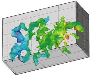
where  $\langle \,\rangle $ denote spatial averaging for Eulerian statistics and averaging over instances of particles for Lagrangian statistics and ς denote standard deviations. For both correlations, the results of k-means-based detection have higher tails, implying that more events with high correlations are captured. Furthermore, examination of time series of structures (e.g. figure 9) indicates that results of the k-means-based detection appear to be more continuous in time and space as well as better correlated. For example, the correlations of λ 2 with pressure are 72 % correlated in successive time steps for clustering-based results, compared with 67 % for the conditionally sampled data. Figure 9 shows three samples of the evolution of detected QSVs colour coded by their pressure (upper row) and streamwise vorticity (lower row). As expected, the QSVs mostly appear as inclined structures that have a negative pressure, i.e. lower than the spatially averaged value in each realization (zero). Some of the structures have positive and others negative streamwise vorticity, that is, they form counterrotating vortices, consistent with the description by Bernal & Roshko (Reference Bernal and Roshko1986).

Figure 8. (a–c) Several t-SNE 2-D representations of the 45-dimensional matrix used for detecting QSVs. The colours indicate the mean-centred and variance-normalized values of the specified quantities ( $\omega$xy, λ 2 and pressure). (d) The corresponding locations selected as QSV indicated as 1.0, and non-QSV as 0.0. (e) A comparison of correlations of negative pressure with λ 2 and $\omega$xy inside QSVs detected by the k means clustering and conditional sampling based on the magnitudes of λ 2 and $\omega$xy.

Figure 9. A sample sequence showing the evolution of detected QSVs at the indicated times colour coded by their pressure (a–c) and their streamwise vorticity (d–f).
Since the measurement resolution is limited to 200 μm, the Kolmogorov length scales are estimated based on the dissipation rate ε calculated from fitting a −5/3 slope to the inertial range of the measured temporal spectra of u 2 (Liu, Meneveau & Katz Reference Liu, Meneveau and Katz1994; Pope Reference Pope2000). Figure 10 provides samples of these spectra for the two speeds averaged over points located in the middle of the shear layer and across the span. The estimated Kolmogorov scales ( $\eta = {({\nu ^3}/\varepsilon )^{1/4}}$) are found to be 62 μm for 1.45 m s−1 and 17 μm for 5.3 m s−1, at least an order of magnitude smaller than the characteristic size of the cavities, and two orders of magnitudes smaller than the vertical extent of the shear layer. The Taylor microscales, estimated as $\sqrt {15\nu (u_i^2)/3\varepsilon } $ (Pope Reference Pope2000), are 2.1 mm at 1.45 m s−1 and 0.6 mm at 5.3 m s−1. Statistics on the size, strength and orientation of the QSVs are presented in figures 11 and 12. To calculate these geometric scales, one must separate structures that are connected by ‘weak’ links, defined as cases with relatively large cumulative distances from nearby non-zero voxels in all directions. Using a Matlab-based watershed transformation (Meyer Reference Meyer1994), the structures are ‘broken’ at the ridge lines, where the distributions of distance have local maxima. The length of vortices is determined based on the largest eigenvalue of the $\omega$xy-weighted second central moments of the volume, namely the tensor ${M_{ij}} = \iint {{({x_i} - {{\bar{x}}_i})}^2} {{({x_j} - {{\bar{x}}_j})}^2}{\omega _{xy}}({x_i},{x_j})\,\textrm{d}{x_i}\,\textrm{d}{x_j} /\iint {{\omega _{xy}}({x_i},{x_j})\,\textrm{d}{x_i}\,\textrm{d}{x_j}}$. The other two eigenvalues define the cross-section and an equivalent diameter is obtained from their norm. The characteristic strength is estimated by multiplying the spatially averaged $\omega$xy within the vortex with the cross-sectional area. The lengths and diameters of the contiguous regions of low pressures inside the QSVs are also determined by retaining regions where the pressure p falls below specified thresholds, namely Cp = p/0.5 $\rho$U 2 < 0, Cp < −0.1, and Cp < −0.2 and recalculating the eigenvalues of the second central moment of this volume. The 3-D orientations of the structures are based on the eigenvectors associated with the largest eigenvalues.

Figure 10. Frequency (f) spectral density of the streamwise velocity fluctuations at y/h = −0.17, averaged over the entire span and axial extent of the tomographic PIV sample volume. Dashed line is a −5/3 slope fit used for estimating η.

Figure 11. Joint probability densities in a logarithmic scale of the QSV length and diameter at 1.45 m s−1 (a–c), and 5.3 m s−1 (d–f) for: (a,d) QSVs, (b,e) negative pressure (Cp < 0) regions within the QSVs and (c,f) low pressure (Cp < −0.1) regions within the QSVs. Black and red lines indicate aspect ratios of 2 and 5, respectively. (g,h) Conditional PDFs, at the velocities indicated in the legend, of the: (g) diameters, and (h) aspect ratios of the QSVs, low pressure regions in them and the cavities.

Figure 12: Comparisons between PDFs of the separation between two adjacent low pressure regions, conditioned on Cp < −0.1, at U = 1.45 and 5.3 m s−1, and the distance between two cavitation events along the same QSV at U = 10.5 and 16 m s−1.
The most likely diameter of the  $\omega$xy weighted QSV is 1.25 mm and its length is 2 mm for both speeds (figure 11a,d). However, a significant fraction of the data has aspect ratio falling between 2 and 5, with diameters extending to 4 mm, albeit with low probability. With increasing speed, the fraction of structures with diameters exceeding 2 mm and lengths over 10 mm increases. As expected, the regions with Cp < 0 (figure 11b,e) and Cp < −0.1 inside the QSVs (figure 11c,f) are smaller than the entire QSVs. For both thresholds, the most probable low pressure zones have a diameter of approximately 0.2 mm, and an aspect ratio of around 2, but values extend to 5 at both speeds. However, at the higher speed there are more QSVs with diameters exceeding 2 mm and aspect ratios larger than 2 (figure 11a,d) as well as structures of the same size with negative pressures (figure 11c,f). These trends are consistent with those shown by the cavities in figure 7(a). Also like the cavities, the largest aspect ratio (~5) occurs for structures with diameters up to about half of the maximum. However, the different trends with velocity vanish in the Cp < −0.1 plots (figure 11c,f). The PDFs comparing the diameters and aspect ratios of cavities with those of the QSVs and the low pressure regions within them are presented in figures 11(g) and 11(h), respectively. The cavity diameters are smaller than those of the QSVs, as one would expect, consistent with trends observed previously for tip vortices (Choi & Ceccio Reference Choi and Ceccio2007; Pennings, Westerweel & van Terwisga Reference Pennings, Westerweel and van Terwisga2015). As the pressure thresholds are lowered, the most probable diameters of low pressure zones shift from 1.2 mm, the characteristic size of the entire QSVs, to 0.2 mm, matching the characteristic diameters of the cavities at both velocities. The low-probability largest diameters also approach those of the cavities with decreasing pressure threshold, matching them for Cp = −0.2. The most probable aspect ratios of the cavities are smaller than those of the QSVs (figure 11g) owing to the presence of the ‘small spherical’ cavities during the initial growth phase. On the high end, the aspect ratios of the cavities are larger than those of the QSVs. However, as the pressure threshold is lowered, the aspect ratios of the low pressure regions extend to higher values, nearly matching those of the cavities at 16 m s−1, and exceeding those at 10.5 m s−1. Furthermore, statistics of the distance between pressure minima along the QSV, conditioned on Cp < −0.1, are compared with the distance between cavitation events along the vortex in figure 12. The most likely separation between events is around 0.2h of either the pressure minima or the cavities, consistent with the sample visualizations in figures 6 and 9, although the pressure-based modes are slightly smaller. The peaks are broad, and a significant fraction of the data extend to 0.6h, where both PDFs increase with velocity. In summary, the dimensions of the cavities and the distance between them match those of the low pressure regions within the QSVs. These agreements provide strong evidence that the spatial distribution of the early cavitation events is influenced significantly by the pressure field.
Figure 13(a) presents the normalized strength of the vortices. The most probable structures have a strength of 0.06Uh at both speeds. While most of the PDFs for the two speeds collapse, they diverge at strengths exceeding 0.4Uh, where the probability increases with velocity. The characteristic strength of spanwise vortices can be estimated as Uδw, where δw is the vorticity thickness (Brown & Roshko Reference Brown and Roshko1974), defined as  $U/{(\partial u/\partial y)_{max}}$. Based on the mean velocity distributions, at the present site δw = 0.65h and 0.7h for U = 1.45 and 5.3 m s−1, respectively. Hence, the most probable strength of the QSVs is approximately 10 % of those of the spanwise vortices, consistent with previously reported levels (Bell & Mehta Reference Bell and Mehta1992). However, the extreme values, representing e.g. less than 0.1 % of the structures, have strengths (0.65Uh at 1.45 and 0.74Uh at 5.3 m s−1) that are comparable to those of the spanwise structures. As noted above, this is the range where the probabilities are velocity dependent (figure 13a). Statistics on the orientation of the QSVs with aspect ratios over 2 are presented in figure 13(b) as the angle with the laboratory coordinate system. Results for the two velocities appear to be remarkably similar. The angles with respect to the x directions are preferentially small and most likely to be 15°–30°. The structures are likely to be perpendicular to the spanwise directions, and to a lesser extent to wall-normal directions as well. Applying pressure thresholds does not change the trends and are, therefore, not presented. The corresponding statistics of the orientation of the cavities in the region of tomographic PIV data are presented in figure 13(c). Their preferred orientations include small angles to the streamwise directions with a peak around 30°. Like the QSVs, close to perpendicular directions to the spanwise are preferred. However, the cavities have with almost zero probability of being vertical or <30° with preference for angles of 60–70°, remaining significant up to 90°.

Figure 13. The PDFs of the QSV: (a) strength, and (b) angles (in degrees) with the x, y and z directions at U = 1.45 and 5.3 m s−1; and (c) PDFs of the corresponding angles of the cavities.
The statistics of pressure in the shear layer are provided in figure 14. Figure 14(a) compares the PDFs of pressure inside and outside the QSVs, with the latter representing about 83 % of the entire data. All the PDFs are nearly symmetric, with the tails being more intense than Gaussian distributions with same mean and standard deviation (also shown). These trends are consistent with previously published data on pressure fluctuations in turbulent shear flows (Brandao & Mahesh Reference Brandao and Mahesh2022). In contrast, for isotropic turbulence, the PDFs are non-symmetric with longer negative tails, which increase with Reynolds number (Bappy et al. Reference Bappy, Carrica and Buscaglia2019). The pressures are lower inside the QSVs, with similar shifts for both velocities, generally scaling with U 2. Consequently, a pressure coefficient of −0.2 is over 7 times more likely to appear inside the QSV than outside of this vortex. The tails of the pressure fluctuations both inside and outside of the QSVs are larger at 1.45 m s−1 than those at 5.3 m s−1. Based on the trends of inception indices in shear layers reported in Katz & O'Hern (Reference Katz and O'Hern1986), the inception indices at the current Reynolds numbers of velocity measurements are expected to fall in the 0.2 to 0.4 range, in agreement with the magnitudes of the present pressure minima. Recall that the present cavitation inception tests with indices in the 0.5 to 0.6 range are performed at higher Reynolds numbers. These values are also in agreement with the trends reported in Katz & O'Hern (Reference Katz and O'Hern1986). Moreover, the magnitudes of pressure minima are consistent with those of Rankine vortices with the same size and strength as those of the QSVs. For example, a Rankine vortex consisting of a solid body rotation core with diameter D of 1.2 mm and strength  $\varGamma$ = 0.06Uh surrounded by an irrotational flow, has a core pressure coefficient (pressure $\textrm{drop} = \rho {(\varGamma /{\rm \pi} D)^2}$) of −0.17. Furthermore, using Cp = −0.3 to represents the pressure minimum in the core of QSVs at 5.3 m s−1, following Choi & Ceccio (Reference Choi and Ceccio2007), the expected growth rate of cavities along the QSV axis should be 1.65U. This value agrees with the presently measured rates at 10.5 and 16 m s−1 (figure 7c). Figure 14(b) provides the temporal pressure spectra at y/h = −0.17, averaged over the streamwise and spanwise directions. At both speeds, the spectra peak at Strouhal numbers of 0.2–0.3, as discussed in several previous studies, including Driver et al. (Reference Driver, Seegmiller and Marvin1987), which relate it to flapping of the shear layer. In the inertial region beyond this peak, the spectral decay has a slope of −1.6, consistent with that of a turbulent boundary layer (Tsuji et al. Reference Tsuji, Fransson, Alfredsson and Johansson2007). Additionally, at 5.3 m s−1, there are a few low-frequency peaks, which Rockwell & Naudascher (Reference Rockwell and Naudascher1979) have attributed to intermittent switching of oscillatory modes based on kinetic energy spectra.

Figure 14. (a) The PDFs of the pressure inside and outside the QSVs. Black curves are Gaussian distributions with the same mean and standard deviation as those of the pressure at U = 5.3 m s−1. (b) Pressure spectra averaged over the spanwise and streamwise directions at y/h = −0.17.
To evaluate the effect of vortex stretching on the pressure, the statistics of the stretching term along the vortex axis are presented in figure 15. Vortex stretching has been associated with the energy cascade and intermittent formation of regions with high velocity gradients (Taylor Reference Taylor1938; Buaria, Bodenschatz & Pumir Reference Buaria, Bodenschatz and Pumir2020) and formation of pressure minima in vortices (Chang et al. Reference Chang, Choi, Yakushiji and Ceccio2012). Figure 15(a) presents PDFs of  $\varPhi$ inside and outside of the QSVs. Stretching (and contraction) inside the QSVs are much higher compared with those in the surrounding at both speeds, and once scaled with ${(U/h)^2}$, results collapse. Stretching events ( $\varPhi$ > 0) are more frequent than contractions everywhere, a typical feature of turbulent flows owing to buckling of vortices during contraction (Rogers & Moin Reference Rogers and Moin1987). Nonetheless, the QSV contains regions of both significant compression and stretching, consistent with Verzicco & Jimenez (Reference Verzicco and Jimenez1999). Figure 15(b) presents PDFs of the correlations between pressure and the stretching term at the same time and location, with the pressure conditioned on being negative and the stretching on being positive (stretching). Clearly, the PDFs corresponding to the interior of the QSVs are substantially broader than those of the surrounding flow, indicating that in some cases, pressure minima co-occur with high stretching, as one would expect, yet in other cases, they are not. These findings have led to a detailed analysis of the evolution of pressure and stretching inside the QSVs and the relations between them based on Lagrangian statistics. Figure 15(c) shows PDFs of the axial strain rate magnitude inside the QSVs. Similar to other ensemble-averaged turbulence statistics, the vortex axial straining magnitudes scale with U/h, with the most probable values fall in the U/h to 2U/h range. These magnitudes are consistent with the shear strain along the periphery of spanwise vortices with strength of 0.65Uh, and radius of 0.32h, hence core azimuthal velocity of 0.32U and strain rate of U/h.

Figure 15. (a,b) The PDFs of the: (a) vortex stretching term, and (b) correlations between negative pressure and positive stretching; (c) PDFs of the axial strain rate in the QSVs.
Statistics on the instantaneous alignment of the vorticity relative to the principal strain rate directions are presented in figure 16(a,b). As shown in previous studies (Ashurst et al. Reference Ashurst, Kerstein, Kerr and Gibson1987; Tsinober, Kit & Dracos Reference Tsinober, Kit and Dracos1992), the vorticity is preferentially aligned with the intermediate strain rate. This phenomenon is slightly more pronounced inside the QSVs, consistent with the previously observed increase in alignment with the intermediate strain, as the vorticity magnitude increases (Huang Reference Huang1996; Buaria et al. Reference Buaria, Bodenschatz and Pumir2020). There is no significant alignment preference with the most extensive strain, and the vorticity is preferentially perpendicular to the most compressive eigendirection with a slight increase inside the QSVs. Next, we examine the alignment of the QSV structure relative to the principal strain rate directions (figure 16c) and the vorticity (figure 16d). Since the QSV structure is often curved, its alignment is defined based on the direction of the largest eigenvector of Mij introduced previously. Figure 16(c) shows that the QSVs are more likely to be aligned with the most extensive strain rates eigenvector and less likely to be aligned with the intermediate strain direction in comparison with the trends of the vorticity (figure 16a,b). Yet, overall, the QSVs are still preferentially aligned with the vorticity (figure 16d), with the distribution being quite broad. In terms of structure, the PDFs of the strain state parameter (figure 17) confirm the previously published preference for axisymmetric extension (Lund & Rogers Reference Lund and Rogers1994), i.e. a pancake shape. However, this preference is lower inside the QSVs, implying that they contain more axisymmetric contraction events, as one would expect for stretched vortices. All the alignment and configuration trends at the two velocities are remarkably similar. The evolution of s* with time in the same vortex is discussed later based on Lagrangian statistics.

Figure 16. The PDFs of the cosines of the angles between the: (a) vorticity and the principal strain rates outside, and (b) inside the QSVs; (c) the QSV axes and the local principal strain rates, and (d) the QSV axes and the local vorticity. Here, s 1, s 2 and s 3 are the most extensive, intermediate and most compressive strain rate eigenvectors, respectively.

Figure 17. The PDFs of the strain state parameter (Lund & Rogers Reference Lund and Rogers1994). As illustrated, 1 indicates a ‘pancake’ structure, and −1, a stretched vortex.
Next, we examine the impact of viscous diffusion in a direction perpendicular to the vortex axis on the evolution of the QSVs. The ratio of viscous diffusion  $(\nu {\nabla ^2}\omega )$ to axial vortex stretching terms, which are presented in figure 18(a), is typically smaller than one. For the majority of the cases, as long as one does not consider the temporal variations in the strain field (discussion follows), the impact of viscous diffusion is significantly smaller than that of the vortex stretching, especially at 5.3 m s−1. However, in a few cases, the two terms become comparable, much more so at 1.45 m s−1. Furthermore, the present structures are very rarely stretched to the viscous diffusion limit, referring to a situation where the viscous diffusion is equal to the stretching, hence the vortex core cannot shrink owing to stretching. For an axisymmetric vortex, such situation occurs when $4\nu U/hD_\mu ^2 = \varPhi$, where Dμ is the minimum diameter. Figure 18(b) provides the PDF of the instantaneous ratio of Dμ to the actual vortex diameter for the entire QSV data. As is evident, the stretching limit is rarely reached. Note, however, that the relative significance of viscous effects increases with decreasing Reynolds number.

Figure 18. The PDFs of the ratio of the: (a) radial viscous vorticity diffusion in the QSVs to the axial stretching, and (b) the diameter at the axial stretching limit to the measured QSV diameter.
Lagrangian statistics: the analysis in a Lagrangian framework examines the durations and sequence of events underlying the development of pressure minima. With this aim, 105 synthetic, neutrally buoyant, initially randomly distributed particles are tracked in time for the entire 2 s duration of data acquisition. Their trajectories are determined by using a fourth-order Runge–Kutta integration of the local velocity. Particles that leave the field of view are re-seeded at the upstream boundary of the sample volume, while ensuring there is no bias in their spatial distributions by diluting regions with increased concentration of particles. To investigate how long the low pressure events last, figure 19 shows the fraction of time all the particles experience pressures below the specified threshold levels plotted versus their dimensionless durations. This procedure is similar to the analysis reported in Bappy et al. (Reference Bappy, Carrica and Buscaglia2019) based on DNS data of isotropic turbulence. The experimental durations are truncated by the residence time of particles being translated through the sample area at the free-stream velocity, namely 1.2h/U. In figure 19(a) the results inside and outside of the QSVs for the higher velocity are compared, and figure 19(b) shows the effect of velocity for the interior of QSVs. The dotted vertical lines mark the measured initial cavitation growth time, ~0.2h/U, samples of which are presented in figure 7(b). As expected, the time fractions decrease with decreasing pressure threshold. For the same speed, the low pressure events inside the QSVs last significantly longer than those outside of them (figure 19a). Some of the durations are longer than the initial growth time, but most of them (~80 %) are not. Trends in the effect of velocity appear to depend on the threshold level. For a mild pressure threshold (−0.05 and −0.1), the time fractions are higher at 5.3 m s−1 than those at 1.45 m s−1. However, as the threshold is reduced to –0.15 the difference between them diminishes. For all thresholds, the slopes are persistently milder at the higher velocity, implying that the long duration events are more likely to occur at 5.3 m s−1. Bappy et al. (Reference Bappy, Carrica and Buscaglia2019) also show that trends of the frequency of low pressure events with Reynolds number reverse with increasing duration for isotropic turbulence. They decrease with Re for short durations, consistent with the present findings, but they increase for long durations. Unfortunately, we cannot increase the present range of durations without increasing the field of view, hence compromising spatial resolution.

Figure 19. The time fraction of the indicated low pressure events and their durations: (a) inside and outside of the QSVs at 5.3 m s−1, and (b) inside the QSVs for the two speeds. The dotted vertical lines indicate the scaled initial growth times of the cavities.
The Lagrangian correlation of pressure at time t with various quantities at time t + Δt for both speeds, inside and outside of QSVs, are provided in figures 20 and 21. Figure 20(a) shows that the unconditioned pressure–pressure correlations remain above 0.4 for 1.45 m s−1 and 0.5 for 5.3 m s−1, for durations up to 0.8h/U. However, the slopes of all the correlations indicate a more rapid decay for durations of less than 0.2h/U. At longer times, the correlations inside and outside the QSVs start to deviate, with those outside of the QSVs decreasing at a faster rate compared with those inside. Figure 20(b) provides the pressure–pressure correlations conditioned on Cp < −0.05 at both times. These correlations decay at faster rates than the unconditioned results, and the differences between the interior and exterior of the QSVs start at Δt = 0. These trends are consistent with the longer durations of low pressure events inside the QSVs (figure 19a). Here again, the decay rates of the correlations become distinctly slower at Δt > 0.2h/U. For the most part, the correlations increase with velocity, especially at short times. At Δt<0.2h/U, the differences are significant, but they diminish at Δt > 0.8h/U. The differences inside the QSVs are smaller in the conditional statistics (figure 20b), also consistent with the trends depicted in figure 19(b). In summary, the pressure–pressure correlations decrease at a faster rate for short durations, during which the correlation increase with velocity. The variations with velocity diminish for longer times.

Figure 20. Lagrangian pressure–pressure correlations inside and outside the QSVs at the indicated speeds for: (a) the entire data, and (b) conditioned on Cp < −0.05.

Figure 21. Lagrangian correlations of pressure at time t (conditioned on Cp < −0.05 and  $\omega$xy > 5U/h) with the following quantities at time t + Δt: (a) $\omega$xy (b) axial vorticity stretching and (c) contraction inside and outside of QSVs. (d) The average strain state parameter at time t + Δt.
Figure 21(a) provides the pressure– $\omega$xy correlations conditioned on Cp < −0.05 and $\omega$xy > 5U/h for positive and negative Δt. The correlation magnitudes are generally low (<0.2), but are higher inside the QSVs. As expected, they peak at Δt = 0, indicating that low pressure events preferentially co-occur with elevated $\omega$xy only inside the QSVs. While the peak value at 5.3 m s−1 is lower than that at 1.45 m s−1, the correlations at 5.3 m s−1 remain elevated for a longer duration, implying that the pressure minimum and (presumably associated) vorticity maximum last for a longer time. The correlations of low pressures with axial vorticity stretching and contraction events are shown in figures 21(b) and 21(c), respectively. Outside the QSVs, the correlations remain low irrespective of time. However, inside the QSVs the correlations with contraction peak at Δt = 0.2h/U and those with stretching between −0.2h/U and −0.8h/U. These trends suggest that low pressure events in the QSVs preferentially involve a dynamic process consisting of a period of stretching with duration of about 0.6h/U, followed by a period of low pressure, ending with a contraction event. Conditional sampling based on the evolution of straining (not shown) confirms that the pressure decreases during the period of peak straining, reaching minimum when as the straining diminishes.
The Lagrangian evolution of average (over all particles) strain state parameter when the pressure coefficient at time t is lower than −0.05 are presented in figure 21(d). As shown earlier, the QSVs have lower values of s* compared with the surrounding flow, corresponding to a reduced tendency for axisymmetric extension. Starting from Δt ~ −0.6h/U, around the time where the vortex stretching starts (figure 21b), s* decreases, reaching a minimum at Δt ~ 0.2h/U, at the time of peak contraction. These observations suggest causal relationships between vortex stretching and increased tendency towards axisymmetric contraction inside the QSVs. The same trends, but with persistent higher s*, are observed in the surrounding flow. Before concluding this section, one should note that in contrast to the pressure–pressure correlation, all the Lagrangian correlations presented in figure 21(a–c) are more prominent at 1.45 m s−1 compared with those at 5.3 m s−1. The primary cause involves local fluctuations in the magnitudes of vorticity and stretching, which are larger at the high velocity, presumably owing to the higher turbulence level. When the vorticity and stretching term are spatially filtered using e.g. a 3-D Gaussian filter with standard deviation of 0.2 mm, the correlation magnitudes increase, and the differences in correlation between the two speeds diminish, as illustrated in figure 22. The time delay of the peaks in the stretching–pressure and contraction–pressure correlations are longer at 5.3 m s−1, consistent with the longer durations of the vorticity–pressure correlations (figure 22b).

Figure 22. Lagrangian correlations of pressure at time t (conditioned on Cp < −0.05 and  $\omega$xy > 5U/h) within the QSVs with the following spatially filtered quantities at time t + Δt: (a) axial vorticity stretching, (b) $\omega$xy and (c) axial contraction. The spatial filter involves a 3-D Gaussian filter with standard deviation of 0.2 mm.
The time scales of minimum pressure and associated stretching and peak vorticity events are examined next. Figure 23 provides the changes to the magnitude of the average pressure over time, ΔCp = Cp(t + Δt) − Cp(t), as well as the corresponding average stretching term  $\varPhi$ (positive or negative) and vorticity $\omega$xy for the same particle group within the QSV. Errors estimated based on bootstrapping by dividing the data into 5 sets are also presented. Similar to the correlations, the data are provided for when a pressure minimum for each particle trajectory occurs at Δt = 0. Only cases where minimum pressure coefficient is below −0.05 and instantaneous $\omega$xy exceeds 5U/h are considered. The average pressure minimum at 1.45 m s−1 is deeper compared with that at 5.3 m s−1, but this minimum develops and decays at a significantly faster rate. The time scale of the exponential decay rate is 0.11h/U at 1.45 m s−1 vs. 0.28h/U at 5.3 m s−1. These trends with velocity, and the magnitudes of time scales, are consistent with those of the initial decrease in pressure–pressure Lagrangian correlations (figure 20b), i.e. 0.2h/U. While the pressure-conditioned average stretching is always positive, it peaks at Δt ~ −0.5h/U, and then decreases monotonically until Δt ~ +0.3h/U, the timing of peak conditional contraction. The duration of transition is clearly longer than that of the change in pressure. Another result of note is the time delay between two stretching peaks, ~1.5h/U (figure 23b), which appears also in the Lagrangian pressure–stretching and pressure--contraction correlations (figure 22a,c, respectively). The average vorticity peaks when the pressure is minimum and the trends of vorticity are nearly identical for the two speeds. In summary, it appears that the dynamic changes to the vortex pressure and strain fields involve two time scales, a shorter time over which the pressure decays, and a longer time consistent with the stretching–contraction cycle. While the latter is independent of the Reynolds number (figure 23b), the shorter time scales of pressure decay increase with velocity.

Figure 23. Lagrangian evolution of: (a) pressure change, (b) stretching and (c) vorticity when Cp is minimal at Δt = 0 (conditioned on Cp < −0.05 and  $\omega$xy > 5U/h) at U = 1.45 and 5.3 m s−1. The error is determined from a bootstrap analysis involving 5 different subsets.
The next discussion describes our attempt to understand the flow mechanisms affecting the spatio-temporal evolution of pressure and straining in the QSVs. The following analysis, therefore, describes the length scale of events along the QSV axis. To find the QSV axis, after applying the watershed transformation as described before, the vortex is skeletonized (Lee, Kashyap & Chu Reference Lee, Kashyap and Chu1994), i.e. reduced to a line or line segments defining its centre, which is not necessarily the centre of vorticity. This step is only used for identifying the ends of the vortex segment, and for determining whether the vortex contains multiple branches. Then, starting from the detected ends in the case of multiple branches or the centroid in the case of a single branch, the ‘vortex axis’ is built by marching by a distance of 100 μm along the local (total) vorticity vector until a boundary of the structure is reached. This process is repeated for each vortex segment. This axis is evolved in time by displacing synthetic particles located less than 50 μm away from the axis according to the local velocity to determine its next location. The result is compared with the location of the detected QSV axis in the next frame. Due to limitations in spatial resolution, the displaced axis based on particle motion and that determined based on the vorticity distribution could be different by up to the grid size of 200 μm. Only particles located less than 100 μm from the detected axis in the next frame (overwhelming majority of them) are used for defining the location of the QSV in the next time step. In cases of discontinuities, the vortex axis in the next frame is used for filling missing segments. Vortex axis locations that do not correspond to segments detected in previous times are treated as new structures, which are then allowed to evolve in time. Figure 24 shows several sample QSV along with their detected centres. The pressure, strain rate, axial velocity, vorticity and vorticity stretching terms along the axes are recorded. Approximately one half of the approximately 60 000 detected QSVs for each velocity are rotating along the flow direction, i.e. ωx is positive, and the other half are opposite to it.

Figure 24. Samples of QSV segments as determined by the k-means clustering (in red) along with their detected axes.
Figure 25 shows the conditionally averaged evolution of pressure and vortex stretching along the same QSV axis at five time steps around a pressure minimum detected at dt = 0. For each time (two with dt < 0 and two with dt > 0, and for dt = 0), we provide the distribution of average pressure and stretching along the axis of the same (displaced) vortex. That means that for all the curves dl defines the distance from the same segment along the vortex axis where the pressure minimum is located at dt = 0. Hence, the displacement of the entire curve represents e.g. propagation of a pressure wave along the vortex axis. The data are conditioned on pressure minima with Cp < −0.05 as well as  $\omega$xy > 5U/h at dt = 0 and ds = 0. Results for the two velocities are presented separately and, owing to the differences in dimensionless time resolutions of data acquisition, the time steps, i.e. values of dtU/h, are different. Both clearly show evidence of a standing wave of vortex stretching. The evolutions of the stretching terms (figure 25b,d) indicate higher than the conditionally average values at dt < 0 (the average is 2.2U 2/h 2 at 1.45 m s−1 and 2U 2/h 2 at 5.3 m s−1), and lower values at dt > 0. These trends are consistent with the results of Lagrangian correlations in figures 21 and 22, which show that the pressure minimum is preceded by a stretching event and followed by a contraction. Based on figure 25, the characteristic wavelength λ of the stretched vortex segment is approximately 2.4 mm at both speeds, approximately twice the most probable diameters of the QSVs (figure 11). Recall that the typical aspect ratio of the QSVs is also approximately 2 (figure 11) In comparison, the Taylor microscales at 1.45 and 5.3 m s−1 are 2.1 and 0.6 mm, respectively. Therefore, the size of the stretched vortex sections is closer to the dissipation scales at 1.45 m s−1. This observation introduces the possibility that differences in viscous effects influence the time scales of low pressure events, as elaborated upon in the discussion that follows. The time variations of pressure decay are the same as observed in figure 23(a).

Figure 25. (a,c) The pressure and (b,d) axial vortex stretching along the QSV axis at the indicated successive times, when the pressure is minimal at dt = 0 and dl = 0 (conditioned on Cp < −0.05 and  $\omega$xy > 5U/h). (a,b) U = 1.45 m s−1 and (c,d) U = 5.3 m s−1.
Elucidating scale effects in QSV dynamics based on the data: in an attempt to elucidate the mechanisms affecting the observed time evolution of low pressure events within the QSVs, we rely on previously published data on the dynamics of deformed vortices (Verzicco & Jimenez Reference Verzicco and Jimenez1999; Pradeep & Hussain Reference Pradeep and Hussain2001; Abid et al. 2002; Moet et al. 2005). Conceptual schematic descriptions of the processes occurring when a segment of a vortex undergoes local stretching are illustrated in figure 26. When the core size and pressure decrease locally (figure 26b), a part of the initially axial vorticity realigns in the azimuthal direction (Abid et al. 2002). In a cylindrical coordinate system depicted in figure 26, this realignment corresponds to the  $\partial {\omega _\theta }/\partial t = {\omega _z}\partial {v_\theta }/\partial z$ term in the vorticity transport equation. This process in effect generates two vortical rings on both sides of the stretched area, or what has been referred to as coiling of vortex lines. Flow induced by the azimuthal rings opposes the initial stretching, eventually causing a contraction (figure 26c). In extreme cases, collision between these opposite sign vortex rings can cause vortex bursting (Verzicco & Jimenez Reference Verzicco and Jimenez1999). Once contracted, a new set of rings forms, which reverses the axial contraction, resulting in an oscillatory motion of stretching and contraction, hence periodic formation of low pressure regions. According to simulations by Abid et al. (2002), the older rings do not decay, but new successive ones with alternating signs form inward of the previous rings. Therefore, the new rings have a stronger effect on the stretching or compression of the axial vortex than the previous generations. Multiple sites of local stretching–contraction cycles could presumably create intermittent islands of low pressure along the vortex, a scenario consistent with the multi-point cavitation events shown in figure 6. The vortex also diffuses, and consequently both the amplitude of its oscillations and its overall strength decay under the influence of viscosity, with the rate of diffusion decreasing with increasing Reynolds number (Verzicco & Jimenez Reference Verzicco and Jimenez1999; Abid et al., 2002). Abid et al. (2002) also show that the vortex response to axial straining is primarily an inertial process, with the frequency of oscillations f, being dependent only on the initial vortex radius R 0, vorticity $\omega$0 and the wavelength of the stretching events λ, namely f = 2.4 $\omega$0R 0/λ. For the present conditions, using a vortex radius of 0.06h (figure 11g) to represent the vortex prior to local stretching, a strength of 0.06Uh (figure 13a), and length of stretching event of λ = 0.24h (figure 25), the predicted frequency is 3.7U/h, i.e. a period of 1.7h/U. This value is consistent with the presently measured period of stretching–contraction events presented in figure 23(b), suggesting that the observed processes are indeed a result of oscillatory vortex reaction to local stretching events.

Figure 26. A schematic showing the evolution of a vortex segment subjected to local stretching: (a) prior to stretching, (b) formation of secondary azimuthal rings that oppose the stretching and cause contraction and (c) formation of rings that oppose the contraction and cause extension.
The next discussion attempts to estimate the changes to the vortex radius as the pressure evolves around the time of minimum pressure. Unfortunately, the present spatial resolution, 0.2 mm, is not sufficient for resolving the time evolution of the vortex radius R during the stretching-contraction events. However, the evolution can be deduced from the pressure measurements. For example, in a Rankine vortex consisting of a rotational core with radius R and a uniform vorticity, the pressure in the centre is  $p = {p_\infty } - 5\rho {\varGamma ^2}/8{{\rm \pi} ^2}{R^2}$. Hence,
 \begin{equation}\varDelta {C_p}/{C_{p0}} + {C_{p\,min}}/{C_{p0}} = {({R_0}/R)^2},\end{equation}
where Cp 0 is the conditionally averaged pressure coefficient before the stretching starts, R 0 is the corresponding initial radius, assumed to be 0.6 mm for the two speeds,  ${C_{p\,min}}$ is the minimum conditionally averaged pressure coefficient and values of ΔCp are provided in figure 23(a). The present values are: Cp 0 = −0.04 and −0.02, and ${C_{p\,min}} ={-} 0.16$ and −0.11 at 1.45 and 5.3 m s−1, respectively. Equation (3.2) allows us to estimate the time evolution of R/R 0 using the measured pressure. The results for both velocities, assuming that stretching begins at Δt = −1.3h/U, are presented in figure 27. It shows that the core radius is almost halved during stretching, decreasing to a size consistent with the core diameter during low pressure events (0.4 mm, see figure 11g). The evolution of the radius can also be evaluated for a vortex subjected to straining and viscous diffusion. The viscosity-induced time evolution of circulation in a Lamb–Oseen vortex is $\varGamma = {\varGamma _0}(1 - {\textrm{e}^{ - {r^2}/4\nu t}})$, where $\varGamma$0 is the vortex strength far from the core (Batchelor Reference Batchelor1967). For this vortex, the radius of maximum tangential velocity is $R(t) = 2.24\sqrt {\nu t} $, i.e. ${R^2}(\varDelta t + 1.3h/U) = R_0^2 + 5.02\nu (\varDelta t + 1.3h/U)$. The viscous terms are significant, e.g. the viscous growth during a period of h/U is 31 % and 16 % of R 0 for 1.45 and 5.3 m s−1, respectively. In addition to the viscous effects, the radius also changes due to vortex stretching and contraction. For a cylindrical vortex element with a constant volume of ${\rm \pi} {R^2}\lambda $, $\textrm{d}R/\textrm{d}t ={-} sR/2$, where $s = 1/\lambda \,\textrm{d}\lambda /\textrm{d}t$ is the axial strain rate. Thus, the axial strain causes an exponential rise or decay of the vortex core radius. Accounting for both straining and viscous diffusion, an approximation for the growth rate of the radius is
 \begin{equation}\textrm{d}R/\textrm{d}t ={-} sR/2 + 2.5\nu /R,\end{equation}
which, for a fixed s over time would yield,
 \begin{equation}{(R/{R_0})^2} = (1 - 5.02\nu /sR_0^2)\,{\textrm{e}^{ - s(\varDelta t + 1.3h/U)}} + 5.02\nu /sR_0^2.\end{equation}
The time evolutions of R/R 0 for characteristic stretching with a strain rate of s = U/h (figure 15c) for a duration of 1.3h/U at both speeds, followed by contraction with the same magnitude and duration, are also plotted in figure 27. As time increases, the changes to the radius at the two speeds diverge owing to differences in viscous effects. The viscosity slows down the reduction in radius during stretching, and enhances its growth rate during contraction. The magnitude and trends with velocity of the pressure-based estimates, and those calculated for the strained viscous vortex, are similar. Differences can be attributed e.g. to our use of a fixed strain rate magnitude throughout the vortex evolution, as opposed to the time-varying s, uncertainty in R 0 and pressure and much higher complexity in the actual system. Results obtained when the viscous term in (3.4) is removed, i.e. for  ${(R/{R_0})^2} = {\textrm{e}^{ - s\varDelta t}}$, also shown in figure 27, are identical for the two speeds. As expected, the inviscid vortex has a smaller radius than the viscous ones. Note that the modelled trends of the QSV radius with Reynolds number are consistent with those of the measured values (figure 11g). While the unconditioned diameters at the two speeds are similar, those of low pressure events decrease with increasing velocity. In summary, this analysis suggests that, despite the nearly identical (scaled) straining and initial QSV diameter, viscous diffusion causes significant differences in the evolution of vortex radius at the two speeds. To understand this trend, note that while the overall Reynolds number of the current shear layer is high, at the scales of the QSVs, the Reynolds numbers are significantly lower, e.g. $\varGamma$/ν is 870 and 3180 at 1.45 and 5.3 m s−1, respectively.

The minimum pressure in the modelled stretched vortex decreases with increasing Reynolds number. For example, for the same initial pressure coefficient of −0.03 (mode of the PDF in figure 14a), the modelled minimum pressure coefficient for s = U/h for a duration of 1.3h/U is −0.09 and −0.1 at 1.45 and 5.3 m s−1, respectively. Since the turbulence, strength of vortices and strain rate scale with U (figures 4, 13a and 15c), it is reasonable to assume that the same trends hold for higher speeds. Accordingly, the characteristic minimum pressure coefficient in the stretched vortices is −0.121 and −0.122 at 10.5 and 16 m s−1, respectively, i.e. the Reynolds number effects diminish under these conditions. To reach the state of early cavitation events at 10.5 and 16 m s−1, e.g. σ = 0.5 (figure 5b), which would require  ${C_{p\,min}} \le - 0.5$, a vortex with the same size and initial pressure has to be subjected to a stretching strain rate of s = 2.2U/h. Based on figure 15(c), such straining is ubiquitous, hence stretching to the cavitation inception levels is consistent with the present data. The modelled time scales associated with low pressure events can also be estimated by relating the radius to Cp (3.2), and using (3.4) for calculating the time required for the (negative) core pressure coefficient to increase from its minimum value to half that minimum during contraction. For the conditions presented in figure 27, this time is 0.34h/U and 0.52h/U at 1.45 and 5.3 m s−1, respectively. These values are of the same order of magnitude but larger than the corresponding experimental ones, 0.12h/U and 0.3h/U, based on the data in figure 23(a). Furthermore, the predicted and measured time scales are consistent with the conditional statistics of durations presented in figure 19. For a threshold Cp of −0.05, similar to the data in figure 23(a), for the same fraction of time (e.g. 2 × 10⁻⁴), the duration at 5.3 m s−1, 0.52h/U, is longer than that at 1.45 m s−1, 0.34h/U (figure 19b). The longer durations with increasing Re are also a likely contributor to the higher Lagrangian pressure–pressure correlations at 5.3 m s−1 (figure 20). Finally, extrapolating the modelled trends to the cavitation speeds, the time scales of low pressure events at 10.5 and 16 m s−1 are 0.56h/U and 0.58h/U, respectively, i.e. they are much closer than those of the pressure measurements. If we extrapolate the experimental durations instead, but still maintain the logarithmic trend predicted by the model, the gap would be significantly bigger, 0.48h/U and 0.62h/U, respectively. In both cases, these time scales are longer than those of the duration of cavitation events, ~0.2h/U (figure 19). With increasing durations of low pressure events, one would expect an increase in the likelihood of cavitation events (figure 5b), and once they occur, longer cavities, consistent with figure 11(h).
3.4 Nuclei dynamics
This section examines how the nuclei spatial distributions with respect to the low pressure regions affect cavitation inception. Figure 28(b–d) provides the number density of bubbles for ‘natural’ seeding for the locations indicated in figure 28(a) at various cavitation indices. The free-stream distributions are quite similar at all speeds and σ, except one case, for U = 16 m s−1 and σ = 0.45, which has a similar distribution, but slightly higher concentrations. These size distributions are also similar in magnitude and slope (−4) to those compiled from prior laboratory and oceanic observations (e.g. Khoo et al. Reference Khoo, Venning, Pearce, Takahashi, Mori and Brandner2020). There are many possible reasons for the slight increase in the highest speed and lowest cavitation index, such as some minor cavitation elsewhere in the test facility. In the recirculation zone, for each velocity, the number density increases with decreasing σ, and the slopes are steeper, indicating higher fractions of small bubbles compared with large ones. Most notable, the concentrations at 10.5 m s−1 are significantly higher than those at 16 m s−1 for all σ, in contrast to the trends of void fractions in the shear layer, which are ~4 times higher at 16 m s−1. This trend is likely related to differences in the absolute mean pressure in the facility, keeping in mind that for the same σ, e.g. σ = 0.5, the pressure at 10.5 m s−1 is 0.46 bar, and that at 16 m s−1 is 1.04 bar. Consequently, while the dissolved oxygen level is nearly the same in both cases (5.5 ppm), the saturation levels of non-condensable gases are different, 130 % at 10.5 m s−1, and 75 % at 16 m s−1. Hence, the water in the test section is supersaturated at 10.5 m s−1 and undersaturated at 16 m s−1. As a result, in the relatively quiescent region in the recirculating zone (0.1U), mass diffusion is expected to increase the number density of detected bubbles at 10.5 m s−1 and decrease it at 16 m s−1. Since some of these bubbles are likely to be entrained into the shear layer, becoming nucleation sites there, one should not be surprised to find higher concentration of small nuclei (<200 μm) at the lower velocity in the shear layer as well. Conversely, the concentration of large bubble at 16 m s−1 exceeds that at 10.5 m s−1, presumably owing to differences in generation by local cavitation events (figure 5b). Indeed, at the high end, the size of these bubbles is comparable to that of the cavities. The slopes of the number density distributions also increase from −5 to −2 with decreasing cavitation index. In summary, the small nuclei concentration in the shear layer is higher at 10.5 m s−1 than that at 16 m s−1, in clear contrast to the void fraction of cavitation events. Hence, availability of nuclei is not the reason for the increase in the number of cavitation events with increasing velocity. These observations support the arguments made in the previous section that the spatial distribution of cavitation events is dominated by the structure of the pressure field, namely the size, shape, location and duration of low pressure events inside the QSVs.

Figure 28. (a) The location of ‘natural’ bubble distribution measurements shown on the spatial distribution of cavities at 16 m s−1 and σ = 0.55. (b–d) The nuclei number densities for the indicated velocities and cavitation indices, all slightly below cavitation inception levels, in the: (b) free stream, (c) recirculation region under the shear layer and (d) shear layer. Dotted lines show the indicated slopes.
To determine how the nuclei distributions are affected by entrainment of free-stream bubbles into the low pressure regions of the shear layer, we compare the spatial and size distributions of bubbles under controlled seeding at a pressure high enough to prevent cavitation behind the step. We intentionally perform experiments at the same pressure to minimize bias caused by mass diffusion, as discussed above. The nuclei number densities at three different speeds (1.45, 10.5 and 16 m s−1) are shown in figure 29(a). Here, the free-stream and shear layer data are presented in the same plot to allow direct comparisons. Note that the size range is quite limited and does not differ significantly from the injection diameter of 60 μm. In general, there are small difference in the free-stream (FS) size distributions with the bubbles at 10.5 m s−1 being slightly larger than those of the other speeds, yet the overall concentrations differ by less than 11 %. The free-stream concentrations do not vary significantly with axial and spanwise location (not shown). Within the shear layer there is minimal difference between the number densities at 10.5 and 16 m s−1, but the concentration at 1.45 m s−1 is smaller in the 50–70 μm size range, presumably owing to weaker entrainment into low pressure regions within eddies.

Figure 29. Data for controlled bubble injection at a mean tunnel pressure of 1.1 bar: (a) nuclei number densities in the free stream, denoted as FS, and in the shear layer (SL) for the indicated velocities. The sample areas are marked in the inset. (b) The corresponding vertical profiles of microbubble concentration.
Vertical profiles of bubble concentrations in the shear layer and the free stream are provided in figure 29(b), this time using a linear scale to highlight differences. The error bars are based on a bootstrap analysis of 5 subsamples. In all cases, the profiles have two maxima, with the larger one located at approximately y/h = 1.2, well above the shear layer. The free-stream concentration is consistent with the bubble injection rate, and by design, the magnitude and location of the bubble concentration peak show minimal effects of velocity. It appears that significant fractions of the injected bubbles end up in the free stream, and do not play any role in cavitation inception. The combined effects of buoyant rise (1.8 mm s−1 for a 60 μm bubble) and vertical pressure gradients, which oppose each other, are not significant to be observed in the free-stream profile. The second and slightly lower peak is located inside the shear layer, in the region of high mean velocity gradients (figure 3), peak Reynolds shear stresses (figure 4) and the same area where cavitation inception is most prevalent. All the concentrations are lower in the shear layer, 35 % of the free-stream values at 1.45 m s−1 and 75 % at the higher speeds, but the characteristic sizes of bubbles are slightly larger. Identification of possible reasons for this trend, e.g. selective entrainment of large bubbles, turbulence-induced rectified diffusion and even residence time in the recirculating region below the shear layer, is beyond the present scope. Note that, for a flow field with similar characteristics, i.e. the same scaled velocity and pressure fields, the actual pressure gradients induced by the shear layer eddies and, therefore, the associated entrainment rates, increase with velocity. At the higher velocities, the maximum concentrations do not differ significantly from each other, and they are both approximately 75 % of the free-stream values. Hence, they do not exhibit trends that would explain the differences in the number of cavitation events. Between the two peaks, especially in the upper edge of the shear layer at this axial location, 0.0 < y/h < 0.5 (figure 4d), the bubble concentration is very low, suggesting that they might have been depleted by entrainment into the middle of the shear layer. It should be noted that Allan et al. (Reference Allan, Barbaca, Russell, Venning, Pearce and Brandner2022) also report an inward entrainment of bubbles, which are injected into the boundary layer upstream of a downstream-facing step, at x/h > 3. They also observe that the nuclei concentration, above a certain threshold, does not seem to have a major effect on the rate of cavitation events.
Other effects can be inferred from the statistics of nuclei distributions and motions, as summarized in figure 30. First, figure 30(a) shows several sample bubble trajectories at 16 m s−1. Close to the free stream, at the upper edge of the shear layer, the bubble trajectories are more likely to be nearly straight. In contrast, deeper in the shear layer, the bubble trajectories become complex, and they appear to slow down and linger for a brief period of approximately 0.1h/U before accelerating again. The trajectory segments where the bubbles are ‘trapped’, i.e. where their speed is lower than 0.06U, are marked in red. This selected threshold is approximately 50 % of the r.m.s. of the liquid vertical velocity fluctuations, 0.12U, based on the 2-D PIV data in figure 4. As is evident, the trapped segments frequently have small radii of curvature, a phenomenon that can be attributed to interactions with the shear layer vortices. Such trapping has been seen at all velocities for approximately 10 % of the nuclei. Characteristic kinked trajectories have also been observed for bubbles entrained by vortex rings (Sridhar & Katz Reference Sridhar and Katz1999). The vertical profiles on the mean bubble streamwise velocity are compared with the liquid velocity in the shear layer in figure 30(b). In the middle of the shear layer, i.e. at −0.5 < y/h < −0.1, where the bubble concentrations and the Reynolds stresses peak, the bubbles are slower than the mean flow at all speeds. Above and below this region, the differences from the mean liquid velocity diminish. The shape and location of the bubble trajectories suggest that the observed trapping is at least one of the mechanisms for the reduced bubble speed. Trends with velocity are difficult to decipher, and do not deviate beyond the uncertainty determined based on bootstrapping. In summary, the sample results in figures 29 and 30 suggest that interactions between bubbles and vortices affect the bubble dynamics to a level that cannot be ignored in assessing the conditions for cavitation inception. There is a considerable increase in entrainment of bubbles into the shear layer as the velocity increases from 1.45 to 10.5 or 16 m s−1. Yet, the concentrations, as well as spatial and size distributions at 10.5 and 16 m s−1 are quite similar. Hence, they do not point at nuclei-related dynamics that affects the observed rates of cavitation events.

Figure 30. (a) Sample trajectories at U = 16 m s−1 containing ‘trapped’ bubbles highlighted in red; and (b) a comparison of the vertical profiles of bubble mean streamwise velocity with that of the liquid. Error bars indicate the standard deviation.
4. Conclusions
This experimental study characterizes the location of cavitation inception and the associated pressure fluctuation statistics in the near field of a shear layer behind a backward-facing step. Results at free-stream velocities of 10.5 and 16 m s−1 confirm that cavitation inception preferentially occurs in the core of quasi-streamwise secondary vortices located at 0.45 < x/xr < 0.75, i.e. upstream of the peaks in turbulence level. Unlike the profiles of mean velocity and Reynolds stress components, which collapse when scaled using the free-stream velocity and reattachment length, the cavitation-induced void fractions and the aspect ratio of cavities at the same cavitation index increase with increasing speeds. The visualizations indicate that cavitation inception takes place intermittently at multiple points along quasi-streamwise vortices, with different events not necessarily occurring at the same time. To understand these phenomena and trends with Reynolds number, this paper examines the interaction of low pressure events in the QSVs with the strain field in the shear layer in Eulerian and Lagrangian reference frames. Constrained by the available equipment (maximum 15 kHz), the 3-D time-resolved velocity measurements are performed at 1.45 and 5.3 m s−1 using tomographic particle tracking, and the pressure distribution is calculated by integrating the material acceleration. Data analysis examines the scaling trends of the size, shape, evolution and durations of low pressure events, and compares them with the configuration of cavities. The QSVs are detected using k-means clustering based on quantities derived from velocity gradients. In addition, we examine the spatial distributions of ‘natural’ and seeded nuclei in and around the shear layer to determine whether they play a significant role in the scaling trends.
Statistical analysis shows that the pressure is lower, and its minima last longer within the QSVs compared with the surrounding flow. The low pressure regions in the QSVs are similar in diameters, aspect ratios and orientations to the cavities. Conditional statistics based on pressure magnitude indicate that with decreasing pressure threshold, the PDFs of the dimensions of low pressure events match those of the cavitation. Like most turbulent flows, the vorticity is preferentially aligned with the intermediate eigenvector of the strain rate tensor. However, this preferred alignment is less pronounced within the QSVs, where there is an increased probability of alignment with the most extensive eigenvector. Compared with the surrounding flow, the QSVs are subjected to both higher axial stretching and higher axial contraction. Occurrence of pressure minima inside the QSVs (but not outside of them) preferentially involves a dynamic process consisting of a period of stretching with duration of approximately 0.6h/U, followed by a low pressure event that lasts approximately 0.2h/U, and ending with a contraction that starts shortly after the pressure minimum. This sequence of events is explained in terms of the response of a vortex segment to local stretching, a topic that has been investigated before in simpler settings. These studies (e.g. Abid et al. 2002; Moet et al. 2005) show that local stretching initiates periodic stretching–contraction oscillations induced by formation of auxiliary vortex rings, which originate from realignment of vortex lines. Consequently, the regions of low pressure are localized and intermittent, and they might occur at multiple points along the vortex at the same or different times. The previously published time period of a vortex undergoing a stretching–contraction cycle matches the presently observed time scales of the straining cycles of the QSVs.
Lagrangian conditional statistics indicate that the decay of pressure minima and pressure–pressure correlations within the QSVs occurs at a slower pace with increasing velocity. In contrast, the time history of straining is independent of the Reynolds number. To explain these trends, it is argued that that, owing to their small size, viscous diffusion, hence the Reynolds number, plays a significant role in the response of the vortex to axial straining and contraction. Specifically, viscous diffusion of the vortex core, which increases its size, hence opposes the effect of axial stretching, decreases with increasing Reynolds number. Consequently, for the same axial straining, the QSV diameter and pressure minimum in its core decrease as the Reynolds number increases. A simple model of the vortex evolution under the combined effects of stretching/contraction and viscous diffusion agrees with the observed growth/decay rate of the pressure minima within the QSVs. Extrapolating the model predictions suggests that the Reynolds number effects on the pressure minima extends to the speeds of the cavitation tests as well, providing a plausible explanation for the Reynolds number scaling trends of cavitation inception.
The potential impact of availability of nuclei in the shear layer has also been studied under ‘natural’ and controlled seeding. Under ‘natural’ seeding and cavitation indices corresponding to inception or low levels of cavitation, the concentrations of nuclei contradict the increase in the rate of cavitation events with the Reynolds number. In fact, owing to the differences in the absolute pressure for the same cavitation index, the water within the shear layer and in the separated region under it is supersaturated with non-condensable gas at the lower speed and undersaturated at the higher speed. Consequently, the concentration of micro-bubbles is much higher at the lower speed, in contrast to the number cavitation events and concentration of large bubbles resulting from the cavitation. Controlled injection of microbubbles into the free stream at pressure well above cavitation inception level results in partial entrainment into the shear layer. Tracking of the microbubbles reveals several other phenomena, such as trapping by vortices, which causes a reduction in the mean velocity of the bubbles compared with the surrounding flow. Increasing velocity from 1.45 to 10.5 m s−1 results in a three times increase in the concentration of entrained bubbles, but the change between 10.5 and 16 m s−1 is small. Hence, availability of nuclei does not seem to be the cause for the observed differences in cavitation inception rates. In conclusion, the observed scaling trends, which are consistent with other studies of cavitation inception in shear layers, are more likely associated with differences in the unsteady pressure field. The present measurements and statistical analysis suggest that they are caused by effect of Reynolds number, or more specifically, viscous diffusion, on the evolution of secondary vortices subjected to axial straining. Future research that would further improve our understanding of the processes involved should follow the time evolution of the pressure and strain fields at the relevant velocities and in a spatio-temporal resolution that captures the vortex core dynamics.
Acknowledgements
K.-H. Kim and Y.-Y. Young are the program officers for the ONR MURI program entitled ‘Predicting Turbulent Multi-Phase Flows with High-Fidelity: a Physics-Based Approach’. The authors would also like to express their appreciation for and remember Y. Ronzhes, who helped with the design and operation of the experimental set-up and whom we lost recently.
Funding
This study has been funded in part by the Office of Naval Research (ONR) under grant number N00014-18-1-2635, and in part by the ONR MURI program entitled ‘Predicting Turbulent Multi-Phase Flows with High-Fidelity: a Physics-Based Approach’.
Declaration of interests
The authors report no conflict of interest.


