


1. Introduction
In many different types of thermal convection, the nature of the force driving fluid motion and the direction of the prevailing temperature gradient can have a paramount importance in determining the properties of the flow. As an example, the different outcome in terms of convective structures and related hierarchy of bifurcations when the cases of a temperature difference parallel or perpendicular to gravity are examined is one of the main reasons for the existence of a fundamental dichotomy in the literature, i.e. the distinction between Rayleigh–Bénard (RB) convection (see, e.g. Clever & Busse Reference Clever and Busse1994; Li & Khayat Reference Li and Khayat2005; Lappa & Boaro Reference Lappa and Boaro2020) and the equivalent buoyancy flow in laterally heated systems (the so-called Hadley problem, Kaddeche, Henry & Ben Hadid (Reference Kaddeche, Henry and Ben Hadid2003), Lappa (Reference Lappa2005a,Reference Lappab), Melnikov & Shevtsova (Reference Melnikov and Shevtsova2005), Gelfgat (Reference Gelfgat2020) and references therein). A similar concept holds if variations of density are replaced with gradients of surface tension: the different orientation of the imposed temperature difference with respect to the free interface (temperature gradient perpendicular or parallel to it) gives rise to two different variants of surface-tension-driven convection, generally known as Marangoni–Bénard (MB) (Nepomnyashchy & Simanovskii Reference Nepomnyashchy and Simanovskii1995; Ueno, Kurosawa & Kawamura Reference Ueno, Kurosawa and Kawamura2002; Lyubimova, Lyubimov & Parshakova Reference Lyubimova, Lyubimov and Parshakova2015; Lyubimov et al. Reference Lyubimov, Lyubimova, Lobov and Alexander2018) and thermocapillary (or simply Marangoni) flow (Shevtsova, Nepomnyashchy & Legros Reference Shevtsova, Nepomnyashchy and Legros2003; Shevtsova, Melnikov & Nepomnyashchy Reference Shevtsova, Melnikov and Nepomnyashchy2009; Kuhlmann et al. Reference Kuhlmann, Lappa, Melnikov, Mukin, Muldoon, Pushkin, Shevtsova and Ueno2014; Lappa Reference Lappa2016, Reference Lappa2018; Gaponenko et al. Reference Gaponenko, Yasnou, Mialdun, Nepomnyashchy and Shevtsova2021), respectively.
These well-established paradigms have instigated much research leading to a significant amount of knowledge. Most of this success has come from the remarkable simplicity of the related kinematic and thermal boundary conditions (smooth surfaces and uniform temperature distributions) and the associated possibility to conduct experiments in well-controlled conditions. At the moment, the results are spread in myriad papers and those who wish to get in touch with the field may consider some relevant books where such knowledge has been collected in a structured way (Koschmieder Reference Koschmieder1993; Getling Reference Getling1998; Colinet, Legros & Velarde Reference Colinet, Legros and Velarde2001; Lappa Reference Lappa2009, Reference Lappa2012). We wish to remark, however, that, although studies on these fundamental modes of convection and the related hierarchy of bifurcations are not showing any obvious sign of reaching a limit yet (relevant investigations being still produced at a constant rate), the need to place part of these efforts in a more practical context has stimulated the development of ‘alternate’ lines of inquiry.
This endeavour, which has not yet been fully explored, has been produced essentially by the ambition (and/or concrete need) to increase the translational applicability of this type of research to technological problems where fluid motion can be brought about by many mechanisms working ‘in parallel’ (i.e. coexisting). This typically happens in circumstances where point-like, spot-like or finite-size (extended in the three-dimensional space) sources of energy are present, and result in a complex distribution of differently oriented gradients of temperature.
Along these lines, box-shaped roughness elements have received appreciable attention in recent years by virtue of their ability to increase the heat transfer in problems of (pure) thermal convection. Relevant applications are connected with the design of electronic boards (where natural convection is generally regarded as a cheap and convenient cooling strategy because it does not require auxiliary electromechanical equipment) and can be found in other areas where buoyant flow is dominant such as solar energy collectors, nuclear reactors, energy storage systems and furnaces or crucibles (Lappa Reference Lappa2017; Lappa & Ferialdi Reference Lappa and Ferialdi2017; Nadjib et al. Reference Nadjib, Adel, Djamel and Abderrahmane2018; Arkhazloo et al. Reference Arkhazloo, Bouissa, Bazdidi-Tehrani, Jadidi, Morin and Jahazi2019; Lappa & Inam Reference Lappa and Inam2020).
For these reasons, the fundamental problem represented by a set of heated elements located on a horizontal adiabatic wall interacting with air or other fluids has been investigated for a variety of circumstances, including (but not limited to) different enclosure aspect ratios, variable horizontal and vertical size of the blocks (with the case of flush-mounted discrete heat sources considered as a limiting condition), different thermal behaviours along the boundary of the enclosure (e.g. cavities with cold top and lateral walls, or with the cooling role played by the sidewalls only, or with asymmetric cooling arrangements, etc.) Related studies conducted under the constraint of two-dimensionality have produced interesting and valuable results in terms of trends and general dependences (e.g. Ichimiya & Saiki (Reference Ichimiya and Saiki2005), Bazylak, Djilali & Sinton (Reference Bazylak, Djilali and Sinton2006), Cheikh, Beya & Lili (Reference Cheikh, Beya and Lili2007), Paroncini & Corvaro, (Reference Paroncini and Corvaro2009), Mukhopadhyay (Reference Mukhopadhyay2010), Naffouti et al. (Reference Naffouti, Zinoubi, Che Sidik and Maad2016), Soni & Gavara (Reference Soni and Gavara2016), Biswas et al. (Reference Biswas, Mahapatra, Manna and Roy2016) just to cite some recent efforts). In comparison, results for three-dimensional (3-D) configurations are more rare and sparse (see, e.g. the experiments by Polentini, Ramadhyani & Incropera (Reference Polentini, Ramadhyani and Incropera1993) and Tso et al. (Reference Tso, Jin, Tou and Zhang2004) and the numerical simulations by Sezai Reference Sezai2000).
As evidenced by all these efforts, for the specific case of mixed forced–buoyant or pure buoyant convection, our knowledge of these phenomena has reached a sort of maturity in the sense that numerical and experimental techniques have successfully led to valuable and relevant information. Unexpectedly, however, this short review of the literature also clearly shows that equivalent findings for the situation in which the flow is significantly affected (or dominated) by surface-tension effects are de facto still missing.
A vast and long-lasting line of inquiry dedicated to surface-tension-driven flows and related instabilities only exists for the case in which the fluid is uniformly heated along one of the boundaries delimiting the fluid domain and this boundary is flat (for the canonical MB convection, in particular, heating is applied from below, Bénard Reference Bénard1900, Reference Bénard1901; Pearson Reference Pearson1958; Cloot & Lebon Reference Cloot and Lebon1984; Bragard & Lebon Reference Bragard and Lebon1993). To the best of our knowledge, only a single relevant analysis has been produced till date where periodically patterned plates have been considered as bottom (hot) wall. Ismagilov et al. (Reference Ismagilov, Rosmarin, Gracias, Stroock and Whitesides2001) conducted a series of interesting experiments along these lines using infrared imaging to observe the emerging planform for different morphologies of the imposed topography (bulges having triangular, square or hexagonal shape or being one-dimensional, i.e. configured as a set of corrugations developing continuously along a fixed direction). These authors revealed that when the convective cells typical of this type of convection form under the same conditions that would produce ‘standard’ MB convection, but over a periodically corrugated or shaped wall, their structure and size essentially depend on two factors, namely, the thickness of the topography and the related symmetry and frequency (i.e. the shape of the bulges and their number per unit length).
The overarching aim of the present study is to continue such inquiry with an eye on the lines of research (illustrated before) where ‘cubic’ items were considered as the elements ‘perturbing’ the flow. Put simply, our objective is to analyse convection driven by gravitational and surface-tension effects in a layer of liquid with a free top interface in the presence of 3-D blocks (rods) of square cross-section (parallelepipedic shapes) regularly arranged at its bottom along two perpendicular horizontal directions (thereby resembling the squares of a checkerboard or the elements of a structured grid).
Obviously, in addition to the purely theoretical implications represented by the inclusion of a new driving force in this specific line of research, the present work also aims to build new information potentially supporting the introduction of new technologies or the advancement of already existing ones. Indeed, micro-patterned surfaces delimiting a liquid in contact with an external gas are critical to the development of moulds or scaffolding for forming ordered microstructures. They can be used as model substrates for a variety of applications in surface science and are at the root of several lab-on-chip devices (Schäffer et al. Reference Schäffer, Harkema, Roerdink, Blossey and Steiner2003; McLeod, Liu & Troian Reference McLeod, Liu and Troian2011; Mayer et al. Reference Mayer, Dhima, Wang, Steinberg, Papenheim and Scheer2015). Another relevant example is represented by the preparation of porous polymer membranes for innovative processes where the biggest challenge is represented by the need to control both the size distribution and the relative positions of the pores (Widawski, Rawiso & François Reference Widawski, Rawiso and François1994; Khan et al. Reference Khan, Wang, Yuan, ul Haq, Wu, Usman, Song, Han and Liu2017). They also find application in controlled release of drugs or other bioactive species (Zhao, Moore & Beebe Reference Zhao, Moore and Beebe2001) and enhanced cell culturing (Wang et al. Reference Wang, Zongkai Yu, Mei and Xue2017). Last but not least, engineered surfaces with topographies that scale favourably at small length scales can be used for the production of nanocrystals (Maillard, Motte & Pileni Reference Maillard, Motte and Pileni2001) or to assemble microscopic particles (Ismagilov et al. Reference Ismagilov, Rosmarin, Gracias, Stroock and Whitesides2001; Balvin et al. Reference Balvin, Sohn, Iracki, Drazer and Frechette2009) or droplets (Widawski et al. Reference Widawski, Rawiso and François1994) into regular lattices; in these applications, the ability to control the fluid-dynamic conditions is the key to obtain desired deposition conditions or to generate lattices with well-defined properties.
2. Mathematical model
2.1. The geometry
As anticipated in the introduction, the hallmark of the present study is the consideration of a ‘patterned’ surface delimiting the considered liquid from below, where the attribute ‘patterned’ is used to describe both the physical morphology of the boundary and its thermal features. Put simply, this fixed imposed topography consists of wall-mounted hot rods with square cross-section (having side length  ${\ell _{horiz}}$) and thickness ${\ell _{vert}}$. Successions of such box-shaped blocks, evenly distributed in space, are implemented along both the x and z (horizontal) directions. As shown in figure 1, this results in a horizontal wall displaying a regular distribution of N×M elements protruding vertically (along the y axis) into the liquid. Depending on the specific perspective taken by the observer, this distribution might also be seen as a set of staggered solids, arranged in N distinct ‘rows’ or M ‘columns’, respectively (a kind of wall ‘roughness’ with well-defined geometrical properties).

Figure 1. Three-dimensional view of the fluid layer hosting an array of square bars resting on the bottom wall (hot blocks), uniformly spaced along the x and z (horizontal) directions (spacing, width and height can be systematically varied).
For the sake of completeness, we consider the two disjoint situations in which the floor (the portions of flat bottom boundary between adjoining elements) is either adiabatic or set at the same temperature Thot as the blocks (hot floor case). This actually enriches the problem with an additional degree of freedom (with respect to those enabled by the possibility to change the spacing among the rods, their number and size).
Not to increase excessively the overall problem complexity, however, the free interface separating the liquid from the overlying gas is assumed to be flat and undeformable. This simplification holds under the assumption that the Galileo and capillary numbers take relatively small values (the related rationale can be found, e.g. in Lappa (Reference Lappa2019b,Reference Lappac) and references therein). These can be defined as  $G{a_c} = \mu {V_r}/\Delta \rho g{d^2}$ and $Ca = \mu {V_r}/\sigma$, respectively, where μ is the liquid dynamic viscosity, g is the gravity acceleration, d is the characteristic depth of the fluid layer, Δρ ≅ ρ is the difference between the density of the liquid ρ and that of the overlying gas, σ is the surface tension and Vr is a characteristic flow velocity, which can be expressed as ${V_g} = \rho g{\beta _T}\Delta T{d^2}/\mu$ or ${V_{Ma}} = {\sigma _T}\Delta T/\mu$ depending on whether buoyancy or Marangoni effects are dominant (βT and σT being the thermal expansion coefficient and the surface-tension derivative with respect to temperature, respectively; ΔT being a characteristic temperature difference). For Gac < 1 or Ca < 1, the non-dimensional deformation δ experienced by a free surface under the action of viscous forces can be estimated in terms of order of magnitude as $\delta = O(G{a_c})$ or $\delta = O(Ca)$, respectively. Following a common practice in the literature, δ can therefore be neglected provided $G{a_c} \ll 1$ and/or $Ca \ll 1$ (see again Lappa (Reference Lappa2019b,Reference Lappac) and references therein).
2.2. The governing equations
In line with earlier studies on the classical MB and RB systems, we rely on the self-consistent framework of continuum mechanics where vital information on thermal convection in liquids (and the related hierarchy of instabilities) is obtained through solution of the balance equations for mass, momentum and energy properly constrained by the assumption of incompressible flow and the related Boussinesq approximation. Moreover, more efficient exploration of the space of parameters is obtained by putting such equations in non-dimensional form, that is, length, time and the primitive variables (velocity  $\boldsymbol{V}$, pressure p and temperature T) are scaled here by relevant reference quantities. In particular, the following compact form:
 \begin{gather}\boldsymbol{\nabla }\boldsymbol{\cdot }\boldsymbol{V} = 0,\end{gather}
 \begin{gather}\frac{\partial \boldsymbol{V}}{\partial t} ={-} \boldsymbol{\nabla }p - \boldsymbol{\nabla }\boldsymbol{\cdot }{[}\boldsymbol{VV}{]} + Pr{\nabla ^2}\boldsymbol{V} - Pr\,RaT\hat{\boldsymbol{n}},\end{gather}
 \begin{gather}\frac{{\partial T}}{{\partial t}} + \boldsymbol{\nabla }\boldsymbol{\cdot }[\boldsymbol{V}T] = {\nabla ^2}T,\end{gather}
corresponds to the following choices: Cartesian coordinates (x,y,z), time (t), velocity (V), pressure (p) scaled by the reference quantities d, d 2/α, α/d and ρα 2/d 2, respectively (where α is the liquid thermal diffusivity). Moreover the temperature (T) is scaled by ΔT, that is, the difference between the temperature of the hot solid elements and the ambient temperature Tref (temperature of the external gas).
Obviously, Pr is the well-known Prandtl number (defined as ratio of the fluid kinematic viscosity ν = μ/ρ and the aforementioned thermal diffusivity α), and  $Ra = g{\beta _T}\Delta T{d^3}/\nu \alpha$ is the standard Rayleigh number. By setting Ra to 0, obviously, excluded are any processes that depend on buoyancy effects. In the present circumstances, fluid convection is also produced by gradients of surface tension, that is, thermocapillary effects. The related driving force can be accounted for through a dedicated equation, which expresses separately the balance of shear stresses at the free surface of the layer. Neglecting the shear stress in the external gas, such a relationship in non-dimensional form simply reads
 \begin{equation}\frac{{\partial {\boldsymbol{V}_S}}}{{\partial n}} ={-} Ma{\boldsymbol{\nabla} _S}T,\end{equation}
where n is the direction perpendicular to the free interface (planar in our case),  ${\boldsymbol{\nabla} _S}$ is the derivative tangential to the interface and Vs is the surface velocity vector. Moreover, Ma is the Marangoni number defined as $Ma = {\sigma _T}\Delta Td/\mu \alpha$. A related number, measuring the relative importance of buoyancy and Marangoni effects, is the so-called dynamic Bond number, namely, $B{o_{dyn}} = Ra/Ma$.
An adequate characterization of the overall problem also requires the introduction of proper non-dimensional geometrical parameters to be used to account for the spatial distribution of the cubic elements and their aspect ratio. These are
 \begin{gather}{\delta _x} = \frac{{{\ell _{horiz}}}}{d},\quad {\delta _y} = \frac{{{\ell _{vert}}}}{d},\quad {\delta _z} = \frac{{{\ell _{horiz}}}}{d},\end{gather}
 \begin{gather}{A_{xbar}} = \frac{{{\delta _y}}}{{{\delta _x}}},\quad {A_{zbar}} = \frac{{{\delta _y}}}{{{\delta _z}}}.\end{gather}
Similarly, the aspect ratios of the entire fluid domain are defined as
 \begin{equation}{A_x} = \frac{{{L_x}}}{d},\quad {A_z} = \frac{{{L_z}}}{d},\end{equation}
where Lx and Lz are the related (dimensional) horizontal extensions. Indicating by N the number of elements along z and by M the corresponding number along x, the non-dimensional distance between adjoining elements can therefore be expressed as
 \begin{equation}{\xi _x} = \frac{{{L_{\textit{x}}} - M{\ell _{horiz}}}}{{Md}} = \frac{{{A_x}}}{M} - {\delta _x},\quad {\xi _z} = \frac{{{L_z} - N{\ell _z}}}{{Nd}} = \frac{{{A_{horiz}}}}{N} - {\delta _z}.\end{equation}
Accordingly, each element indexed as (i,k) can be mathematically represented in the physical (non-dimensional) space as
 \begin{gather} \left. \begin{gathered} (i - 1){\delta_x} + \left( {i - \dfrac{1}{2}} \right){\xi_x} \le x \le (i){\delta_x} + \left( {i - \dfrac{1}{2}} \right){\xi_x}\quad \textrm{for}\;1 \le i \le M\\ 0 \le y \le {\delta_y}\\ (k - 1){\delta_z} + \left( {k - \dfrac{1}{2}} \right){\xi_z} \le z \le (k){\delta_z} + \left( {k - \dfrac{1}{2}} \right){\xi_z}\quad \textrm{for}\;1 \le k \le N \end{gathered}\right\},\end{gather}
and on its boundary with the fluid, we assume
 \begin{equation}\boldsymbol{V} = 0\,\textrm{(no}\;\textrm{slip}\;\textrm{conditions)}\;\textrm{and}\;T = 1.\end{equation}
Along the portions of floor (at y = 0) separating adjoining elements, as anticipated in § 2.1, adiabatic or constant temperature conditions are set, i.e.
 \begin{equation}\frac{{\partial T}}{{\partial y}} = 0,\end{equation}
or
 \begin{equation}T = 1.\end{equation}
Heat exchange of the liquid with the external gaseous environment at the free surface is modelled through the classical Biot number (defined as hd/λ where h and λ are the convective heat exchange coefficient and the liquid thermal conductivity, respectively), i.e.
 \begin{equation}\frac{{\partial T}}{{\partial y}} ={-} BiT.\end{equation}
The lateral boundaries of the fluid domain are considered no slip and adiabatic or periodic boundary conditions (PBC) are assumed there. At the initial time t = 0, the flow is quiescent and at the same temperature as the ambient, i.e. T = 0. As time increases its temperature rises as a result of the heat being exchanged with the heated elements until equilibrium conditions are reached.
In the present work, such heat exchange is quantified through the ‘ad hoc’ introduction of different versions of the Nusselt numbers tailored to account separately for the thermal behaviour of the lateral, top or total surface of each heated element, i.e.
 \begin{align} Nu_{barlateralsurface}^{ik} & = \dfrac{1}{(2{\delta _x}{\delta _y} + 2{\delta _z}{\delta _y})}\left[ \int_0^{{\delta_y}} \int_{{x_i}}^{{x_i} + {\delta_x}} \dfrac{{\partial T}}{{\partial z}} \big|_{z = {z_k}}\,\textrm{d}x\,\textrm{d}y - \int_0^{{\delta_y}} \int_{x_i}^{{x_i} + {\delta_x}} \dfrac{{\partial T}}{{\partial z}}\big|_{z = {z_k} + {\delta_z}}\,\textrm{d}x\,\textrm{d}y\right.\nonumber\\ &\left.\quad + \int_0^{{\delta_y}} \int_{z_k}^{{z_k} + {\delta_z}}\left. \dfrac{{\partial T}}{{\partial x}}\right|_{x = {x_i}}\,\textrm{d}z\,\textrm{d}y- \int_0^{\delta_y} \int_{{z_k}}^{{z_k} + {\delta_z}} \dfrac{{\partial T}}{{\partial x}} \big|_{x = {x_i} + {\delta_x}}\,\textrm{d}z\,\textrm{d}y\right], \end{align}
 \begin{equation}Nu_{bartop}^{ik} ={-} \frac{1}{{{\delta _x}{\delta _z}}}\int_{{z_k}}^{{z_k} + {\delta _z}} {\int_{{x_i}}^{{x_i} + {\delta _x}} {{{\left. {\frac{{\partial T}}{{\partial y}}} \right|}_{y = {\delta _y}}}\,\textrm{d}x\,\textrm{d}z} } ,\end{equation}
 \begin{equation}Nu_{bar}^{ik} = \frac{{Nu_{barlateralsurface}^{ik}(2{\delta _x}{\delta _y} + 2{\delta _z}{\delta _y}) + Nu_{bartop}^{ik}{\delta _x}{\delta _z}}}{{(2{\delta _x}{\delta _y} + 2{\delta _z}{\delta _y}) + {\delta _x}{\delta _z}}},\end{equation}
where
 \begin{equation}{x_i} = (i - 1){\delta _x} + \left( {i - \frac{1}{2}} \right){\xi _x}\quad \textrm{and}\quad {z_k} = (k - 1){\delta _z} + \left( {k - \frac{1}{2}} \right){\xi _z}.\end{equation}
Accordingly, space averaged values are introduced as
 \begin{gather}Nu_{side}^{average} = \frac{1}{{NM}}\sum\limits_{k = 1}^N {\sum\limits_{i = 1}^M {Nu_{barlateralsurface}^{ik}} } ,\end{gather}
 \begin{gather}Nu_{top}^{average} = \frac{1}{{NM}}\sum\limits_{k = 1}^N {\sum\limits_{i = 1}^M {Nu_{bartop}^{ik}} } ,\end{gather}
 \begin{gather}Nu_{bar}^{average} = \frac{1}{{NM}}\sum\limits_{k = 1}^N {\sum\limits_{i = 1}^M {Nu_{bar}^{ik}} } .\end{gather}
3. Numerical method
3.1. The projection method
The set of (2.1)–(2.3) with the related boundary conditions ((2.4) and (2.8)–(2.11)) have been solved numerically using an explicit in time primitive-variable technique pertaining to the general category of ‘projection’ or ‘fractional-step’ methods. An extended description of this class of algorithms can be found in Lappa (Reference Lappa2019a) and/or Lappa & Boaro (Reference Lappa and Boaro2020).
In the present work, convective terms have been treated using the quadratic upstream interpolation for convective kinematics (QUICK) scheme while standard central differences have been used to discretize the diffusive terms. Given the delicate role played by the coupling between pressure and velocity (see, e.g. Choi, Nam & Cho Reference Choi, Nam and Cho1994a,Reference Choi, Nam and Chob) a staggered arrangement has been used for the primitive variables, that is, while pressure occupies the centre of each computational cell, the components of velocity are located at the centre of the cell face perpendicular to the x, y and z axes, respectively (see, e.g. Lappa Reference Lappa1997).
A structured uniform mesh, covering the fluid and all the blocks, has been used; however, no calculations have been performed inside the blocks where the temperature is constant and the velocity is zero (from a purely algorithmic standpoint, this has been implemented by using computational cycles able to distinguish blocks from the fluid on the basis of (2.8)).
3.2. Validation
The validation has been articulated into distinct stages of verification. More precisely, the coherence of the model has been verified through comparison with existing linear stability analyses (LSAs) and earlier nonlinear calculations conducted by other authors. Given the nature of the specific subject being addressed, both the classical problems of MB and buoyancy convection have been considered.
The outcomes of the validation exercise based on the comparison with the LSA for the classical MB problem are summarized in figure 2. In particular, figure 2(a) shows the evolution in time of the maximum velocity of the fluid for different values of the Marangoni number, while the corresponding ‘growth rate’ (determined as the logarithm of the slope of the branch of the velocity profile with constant inclination) is reported in figure 2(b). The latter also includes the value of the critical Marangoni number (for the onset of convection from the initially thermally diffusive and quiescent state) determined through extrapolation to zero of the disturbance growth rate. As the reader will easily realize, this value matches with a reasonable approximation (less than 1.5 %) that obtained with the LSA approach (Pearson Reference Pearson1958; Colinet et al. Reference Colinet, Legros and Velarde2001). The 3-D pattern emerging for a value of the Marangoni number slightly larger than the critical one is shown in figure 3 (presenting the classical honeycomb structure of MB convection).

Figure 2. Profile of maximum velocity as a function of time (a) and related growth rate (b) as a function of the Marangoni number (Pr = 10, layer uniformly heated from below with aspect ratio A = 11.5, Bi = 1, mesh 150 × 25).

Figure 3. Case Pr = 10, layer aspect ratio Ax = Az = 11.5, Ma = 125, Bi = 1, mesh 150 × 25 × 150, PBC: (a) temperature and velocity pattern on the free surface; (b) spectrum of the surface temperature distribution.
For the sake of precision, it should be noted that the definition of the Marangoni number we have used for comparison with the LSA is slightly different with respect to that introduced in § 2.2. While in the present work the ΔT appearing in the expression of Ma is the difference between the temperature of the hot walls and that of the ‘ambient’ (the gas located at a certain distance from the liquid surface, assumed not be disturbed and maintain a constant temperature in time), the LSA considers the effective temperature difference which would be established in the absence of convective effects between the top and bottom geometrical boundaries of the liquid layer, i.e. the uniformly heated bottom wall and the free interface. Therefore, the Marangoni number shown in figure 2 is related to that defined in § 2 through a scaling factor, which in the current theoretical framework is (Thot − Tsurface)/(Thot − Tref), i.e. in non-dimensional form Bi/(Bi + 1) (Eckert, Bestehorn & Thess Reference Eckert, Bestehorn and Thess1998).
These simulations confirm that (as expected) the only effect of a Bi ≠ 0 is to shift the critical Marangoni number (MaLSA ≅ 80 for Bi = 0) and change the growth rates of unstable modes, while the hexagonal planform (figure 3a) is still a stable attractor for the nonlinear governing equations. The related wavenumber determined through analysis of the surface temperature distribution (figure 3b) k ≅ 2.2 is in very good agreement with the prediction by Pearson (Reference Pearson1958) and Colinet et al. (Reference Colinet, Legros and Velarde2001) (the additional wavenumbers visible in the spectrum represent higher-order harmonics with negligible amplitude, which are excited because the considered Ma is slightly larger than the critical value).
As a second step of code verification, we have examined pure buoyancy convection originating from a heated element with rectangular shape encapsulated in (located on the bottom of) a square cavity with adiabatic bottom boundary and cold (isothermal) top and lateral walls. Assuming the same conditions originally investigated by Biswas et al. (Reference Biswas, Mahapatra, Manna and Roy2016), we have tackled four representative conditions corresponding to distinct aspect ratios of the heater and different values of the Rayleigh number (see figure 4 and table 1). As witnessed by these data, a very good agreement holds in terms of Nusselt number.

Figure 4. Temperature and streamlines in a square cavity with heater located on adiabatic bottom and other (lateral and top) walls at constant (cold) temperature (Pr = 25.83, different values of Ra and the heated element aspect ratio); (a) δhoriz = 0.33, Abar = 1.0, Ra = 105 (grid 100 × 100); (b) δhoriz = 0.64, Abar = 0.3, Ra = 104 (grid 70 × 70);
Table 1. Comparison with the results by Biswas et al. (Reference Biswas, Mahapatra, Manna and Roy2016) (see figure 7 in their work), square cavity with heater located on adiabatic bottom and other (lateral and top) walls at constant (cold) temperature (Pr = 25.83, different values of Ra and the heated element aspect ratio).

As a concluding remark for this section, we wish to recall that the computational kernels underpinning the present algorithm have already been used extensively in earlier studies of the present authors (concerned with various realizations of buoyancy and surface-tension-driven convection, see, e.g. Lappa Reference Lappa2019b,Reference Lappac). Accordingly, they were also validated through comparison with other relevant benchmarks and test cases (this information is not duplicated here for the sake of brevity).
3.3. Mesh refinement and related criteria
In order to ensure the judicious use of the available computational resources and, at the same time, produce results which can be trusted, it is known that good practice consists of conducting a thorough and extensive analysis of the sensitivity of the emerging solutions to the used mesh.
Towards the end to reduce the computational cost of the grid independence study itself, in particular, here such a parametric assessment has been initially conducted considering the equivalent 2-D configuration (assumed to have infinite extension along the third direction z) for the same parameters investigated in § 4. Such a strategy rests on the realization that since the 3-D geometry illustrated in figure 1 consists of periodically positioned items along both the x and z directions (i.e. a rotation by 90° would not change the physics of the problem), a 2-D framework should be regarded as a relevant approach for a preliminary estimation of the needed numerical resolution. As sensitive parameters for such investigation, in particular, we have considered both kinematic and thermal quantities, namely, the maximum of the velocity components along x and y, and the spatially averaged (over the considered set of blocks) Nusselt number defined through (2.16) and (2.17). The outcomes of such a parametric investigation for a set of representative cases (Pr = 10, N = 3, 5 and 7, Ma = 5000, Ra = 10 000, Bi = 1.0, δhoriz = 1.0, δvert = 0.3) are summarized in table 2.
Table 2. Grid independence study (2-D configuration, aspect ratio = horizontal length/depth = 10, Pr = 10, N = 3, 5 and 7, Ma = 5000, Ra = 10 000, Bi = 1.0).
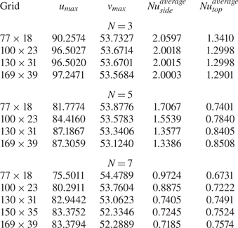
As a fleeting glimpse into a such a table would confirm, although the rate of convergence tends to be slowed down as N is increased, a resolution with ≅30 points along the vertical direction and 130 points along the horizontal one can be considered enough for all these cases (all the percentage variations falling below ≅2 % for a further increase in the mesh density).
To double check that such a resolution can also capture properly the small-scale details of the emerging 3-D pattern (potentially affected by ‘high-wavenumber excitations’ for the considered value of the Marangoni number, Thess & Orszag Reference Thess and Orszag1995), dedicated simulations have been performed for resolution exceeding 130 computational nodes along both the x and z directions. Given the complex nature of the convective structures produced in this case, a quantitative assessment of the results (on increasing the number of points) has been conducted in terms of (spatial) spectrum of the surface temperature distribution.
The related outcomes shown in figure 5 for N = 7, confirm that all the spectra align almost perfectly. Most importantly, the extension of the spectrum does not change on increasing the density of the mesh, neither in terms of amplitude distribution (vertical coordinate), nor in terms of horizontal extension (i.e. the minimum and the maximum values of k). These observations gives us confidence that the used resolution is also sufficient to avoid unresolved regions in the 3-D fluid domain, i.e. it is enough to capture the small-scale behaviour of surface-tension-driven convection for the considered value of the Marangoni number (a denser mesh does not result in the realization of smaller-scale kinematic or thermal features).

Figure 5. Spectrum of the surface temperature distribution for increasing number of grid points in the horizontal direction (Pr = 10, Ma = 5 × 10³, Ra = 104, Ax = Az = 10, Bi = 1.0, N = 7, 3-D numerical simulations, solid lateral walls, spectrum for a temperature profile at x = 2).
We wish to remark that a similar check has also been conducted for N = 5 (the spectrum in this case, not shown, is simpler), leading to the same conclusions, i.e. a grid with ≅130 points is sufficient to obtain convergence in terms of spectrum behaviour. Accordingly, all the simulations presented in the next section have been conducted using 130 × 31 points (corresponding to a total of ≅5 × 10⁵ nodes). As the reader will realize by inspecting the related results, among other things, such resolution guarantees that in all cases the ratio between the number of points in the horizontal direction and the number of convective-cell wavelengths is on average always greater than or ≅20).
4. Results
Without loss of generality we restrict our analysis to Pr = 10 (a value representative of a vast category of high Prandtl number fluids) and unit Biot number (Bi = 1). Moreover, a square layer with relatively large aspect ratio (horizontal extension/depth) is considered, i.e.  ${A_x} = {A_z} = {A_{horiz}} = 10$; accordingly we set δx = δz (hereafter simply referred to as δhoriz, because the heated solid elements have a square basis) and N = M (i.e. the number of elements along x reflects the corresponding distribution of elements along the z direction, and vice versa).
As a key to unlocking the puzzle about the relationship between the emerging pattern and the imposed boundary conditions, we vary parametrically the number of square rods present in the regular array (N × N from 3 × 3 to 7 × 7 passing through intermediate states 5 × 5). Not to increase excessively the dimensionality of the space of parameters, the vertical extension of the rods is fixed to δy = 0.3 (hereafter simply referred to as δvert, corresponding to 30 % of the overall depth of the liquid layer), while three distinct values are selected for δhoriz (namely, 0.1, 0.55 and 1.0). This allows us to change the spacing among the elements while retaining the same overall number N × N. As anticipated in § 2, as an additional degree of freedom, the portions of flat surface (at the bottom) separating adjoining elements are considered adiabatic (thermally insulated) or isothermal (at the same temperature as the heated elements). Moreover, no-slip conditions (finite-size horizontal extension) or PBC (to mimic an infinite layer) are imposed at the lateral boundaries.
Since in the absence of observational information to properly constrain the model parameters, considering asymptotic conditions in which a new problem reduces to already known paradigms is beneficial, we also examine a few cases with uniform heating or a single heat source (heated bar) located in the geometric centre of the physical domain (these two models being obviously opposite extremes with respect to the situations mathematically described by (2.8)). Moreover, towards the end to assess the separate influence of buoyancy and Marangoni effects, the simulations are conducted by setting Ma and Ra to their intended values and ‘switching off’ alternately one of them (the complementary situations with Ma = 0 or Ra = 0 being obviously instrumental in discerning the pure gravitational or surface-tension-driven phenomena). To limit the otherwise prohibitive scale of the problem thus defined, the ratio of the Rayleigh and Marangoni numbers (Bodyn) is fixed to 2, i.e. Ra = 104 and Ma = 5 × 10³ (assuming a realistic Pr = 10 oil with kinematic viscosity ν = 6.5 × 10⁻⁷ m2 s−1, thermal diffusivity α = 6.5 × 10⁻⁶ m2 s−1, density ρ ≅ 0.97 × 10³ kg m−3, thermal expansion coefficient βT = 10−3 K−1, surface-tension derivative σT = 6 × 10⁻⁵ N m−1 K−1, this would correspond to a layer with depth d ≅ 3.5 mm and a ΔT ≅ 1 K).
We wish to remark once again that, in the present work, ΔT accounts for the temperature difference between the bottom plate and the ‘ambient’ (gas) temperature. Using the same definition of the Marangoni number traditionally adopted in the frame of LSA and similar studies on MB convection, the MaLSA corresponding to the present value 5000 would be 2500, which is very close to the case that Thess & Orszag (Reference Thess and Orszag1994, Reference Thess and Orszag1995) examined in the limit as  $Pr \to \infty$ (we will come back to this interesting observation later).
All the simulations have been run for a time sufficiently long to allow the Nusselt number to reach asymptotic (time-independent) values for the cases where the flow is stationary (generally a period corresponding to 4 times the thermally diffusive time based on the depth of the layer, i.e.  ${t_\alpha } = {d^2}/\alpha$). The equations have been integrated with a non-dimensional time step 2.5 × 10⁻⁶ (therefore requiring more than one million of steps for each case). For time-dependent solutions, the simulations have been extended to a non-dimensional time t = 10 (we will come back to the implications of this apparently innocuous remark later). Given the density of the mesh (5 × 10⁵ grid points), three continuous months of calculations have been required using an 8-core workstation to produce all the results reported in the following subsections.
4.1. The purely buoyant case
Following the approach outlined above, a first sub-set of numerical findings for the purely gravitational situation (no surface-tension effects being considered) are presented in figures 6–8. These refer to the situation with adiabatic floor. In particular, figure 6 relates to the simplest possible case, i.e. the configuration with a single block located at the centre.

Figure 6. Temperature and velocity fields for pure buoyancy convection (Ra = 104, Ma = 0, Bi = 1) and single block with δhoriz = 1 (otherwise adiabatic floor): temperature and streamlines distribution at the free interface (a); and isosurfaces of temperature (blue = 0.11, green = 0.22, red = 0.41) shown in combination with two representative bundles of streamlines (b). The bowl shape of the temperature isosurfaces reflects the toroidal structure of the single annular roll established in the cavity; hot fluid is transported from the centre towards the lateral walls at the interface, while relatively cold fluid moves in the opposite direction along the bottom wall. Here,  $N{u_{side}} \cong 6.32$, $N{u_{top}} \cong 5.12$ and $N{u_{bar}} \cong 5.78$.

Figure 7. Survey of patterns (surface temperature distribution) obtained by varying N in the range between 3 and 7 for δhoriz = 1, 0.55 and 0.1 (pure buoyancy convection, adiabatic floor).
Figure 8. Nusselt number as a function of N for the configurations with adiabatic floor and adiabatic lateral solid walls (pure buoyancy convection, the splines are used to guide the eye): (a) δhoriz = 1; (b) δhoriz = 0.55; (c) δhoriz = 0.1.
In agreement with the observations reported in earlier works (see, e.g. the numerical investigation by Sezai Reference Sezai2000), the reader will recognize in this figure the classical convective structure with hot fluid rising just above the top surface of the heated block, reaching the top of the boundary (the free surface exchanging heat with the external gas in our case, as opposed to the solid cold wall considered by Sezai Reference Sezai2000), then spreading radially outward towards the sidewalls where it finally turns downward and moves back in the radial direction towards the source where it was generated.
Following up on the previous point, figure 7 provides a first glimpse of all the considered geometrical configurations and the related (surface temperature) patterns after transients have decayed away when the number of blocks is increased from one to larger numbers. As a property common to many different cases, it can be noticed that for a relatively ‘dilute’ distribution of blocks (i.e. a not too high value of N), each of them contributes to the emergence of a well-defined plume similar to that obtained for N = 1. This is witnessed by the visible presence of a ‘set’ of distinguishable approximately circular spots on the free surface. Each of these warm areas corresponds to the localized region where a current of rising hot fluid meets the liquid/gas interface (where heat exchange with the external environment takes place).
The significance of these figures primarily resides in their ability to make evident that for relatively large spacing of the heated elements, the plumes are independent, i.e. they do not interact and do not coalescence. However, they also reveal that if the spacing is reduced (by increasing N), at a certain stage, non-trivial planforms are produced, i.e. patterns with well-defined properties which do not simply reflect the (a priori-set) order of the underlying grid of hot blocks.
While for δhoriz = 1, i.e. unit horizontal extension of the element side (first row of figure 7), a perfect 1 : 1 correspondence can be established between sources and plumes for both N = 3 and N = 5, for N = 7, as a result of plume interaction the number of recognizable hot spots at the free surface decreases. More precisely, as opposed to situations with smaller N, for which the location of rising currents is simply consistent with the related distribution of heat sources, an external observer looking at the free surface of the configuration with N = 7 would naturally be induced to map the set of plumes into an array with lower dimensions, i.e. a 5 × 5 matrix.
Following up on these observations, very interesting aspects concern the symmetries, which are broken or retained. In such a context it is worth recalling briefly that the considered square configuration with a free surface has the symmetries of the dihedral group D 4, that is, the group of symmetries of a regular polygon with 4 vertices. These include the reflections S 0, S 1, S 2 and S 3 (where the generic Sk is the reflection about the line through the centre of the square making an angle of πk/4 with one of its sides, e.g. the x axis in our case). The chosen disposition of the blocks allows keeping these symmetries, whereas the up–down symmetry is not valid because of the free upper surface and the presence of blocks.
It is interesting to see that all the buoyant cases (figure 7) keep all the symmetries of the D 4 group. The related patterns are also all steady. This suggests that no bifurcation occurs in this case when the size of the blocks is increased and that there is a continuous evolution between the cases with different sizes of blocks, even when the correspondence between the blocks and the surface distribution of hot spots is lost, namely for the 7 × 7 case when δhoriz is changed from 0.55 to 1.
Having completed a description of the emerging patterns in terms of spatial features, we turn now to characterizing these solutions in terms of heat exchange (for which we use the parameters introduced ‘ad hoc’ in § 2). These are reported in an ordered way as a function of N in figures 8(a)–8(c) for δhoriz = 1.0, 0.55 and 0.1, respectively.
As a fleeting glimpse into these figures would confirm, although the trends are all similar, swaps are possible in the relative importance of  $Nu_{side}^{average}$ and $Nu_{top}^{average}$, which require some proper explanations or interpretations. In this regard it is convenient to start from the simple remark that the decreasing behaviour of the different curves (being perfectly monotonic for all cases) should be regarded as a consequence of a thermal saturation effect, i.e. the obvious tendency of the fluid to acquire (on average) an increasingly larger temperature as the number of heating elements (‘heaters’) grows (figure 9). Such an increase obviously tends to weaken the temperature gradients between the elements and the fluid, thereby causing a general decrease in the magnitude of the Nusselt number.

Figure 9. Lateral view (plane xy) for δhoriz = 1 and different values of N (pure buoyancy convection, adiabatic floor and adiabatic lateral solid walls): (a) N = 5; (b) N = 7.
This mechanism is also responsible for the inversion in the relative importance of  $Nu_{side}^{average}$ and $Nu_{top}^{average}$ for δhoriz = 1.0 as N exceeds a given threshold (in figure 8(a), $Nu_{top}^{average} < Nu_{side}^{average}$ or $Nu_{side}^{average} < Nu_{top}^{average}$ for N ≤ 5 or N > 5, respectively). The simplest way to elaborate a relevant interpretation is to consider the emergence of ‘heat islands’, which for δhoriz = 1 tend to be formed in the thin (interstitial) regions located between adjoining elements as N is increased. As an example, see figure 9(b), for N = 7 the temperature in these regions becomes almost identical to that of the elements. In other words, for these specific conditions, the entire set of rods (though physically disjoint) formally behave as they were a single uniformly heated block (having constant thickness and the same horizontal extension of the entire liquid domain). Accordingly, $Nu_{side}^{average}$ drops to a value that is almost negligible.
Although the condition with unit horizontal extension of the elements (δhoriz = 1) is the only one for which  $Nu_{side}^{average}$ becomes almost zero for N = 7 (figure 8a), a similar justification can be invoked for the inversion in the relative importance of $Nu_{top}^{average}$ and $Nu_{side}^{average}$ in the range N ≤ 5 when δhoriz is decreased ( $Nu_{top}^{average} < Nu_{side}^{average}$ or $Nu_{side}^{average} < Nu_{top}^{average}$ for δhoriz ≥ 0.55 or δhoriz < 0.55, respectively). A rationale for this trend can directly be rooted in the realization that while for δhoriz ≥ 0.55 large thermal plumes originate from the top of the heated elements giving rise to vertically extended regions of fluids (figure 10a,b) where the temperature is relatively uniform and close to that of the heat sources (causing a significant weakening of $Nu_{top}^{average}$ with respect to $Nu_{side}^{average}$), for δhoriz = 0.1, such ‘heat islands’ are weaker and, accordingly, the gradient between the top surface of the elements and the overlying fluid is higher.

Figure 10. Lateral view (plane xy) for N = 7 and different values of δhoriz (pure buoyancy convection, adiabatic floor and adiabatic lateral solid walls): (a) δhoriz = 1; (b) δhoriz = 0.55.
Obviously, the aforementioned thermal saturation effect is enhanced if the portions of adiabatic floor located among adjoining elements are replaced with equivalent portions of isothermal (hot) wall. Such a swap in the thermal boundary condition at the bottom causes an appreciable decrease in the block Nusselt number (this being quantitatively substantiated by the data summarized in table 3, where the values of Nu can be compared for different thermal behaviours of the floor and equivalent geometrical conditions, i.e. same values of N and δhoriz for some representative cases).
Table 3. Comparison between the Nusselt number obtained for configurations with adiabatic and hot bottom wall (Ra = 104, Ma = 0).

Notably, the differences are not limited to a variation in the magnitude of the heat exchange taking place between the elements and the fluid. The changes can be substantial and affect the entire structure of the flow, especially if one considers configurations with small δhoriz. This conclusion is supported by cross-comparison of the patterns in figure 11. Moving on from the case with adiabatic floor to that with hot floor, it can be seen that, although some localized plumes originating from the hot blocks still manifest as independent flow features, in the latter case the overall pattern tends to take a configuration very similar to that with three main plumes along each wall, which is obtained when the equivalent (classical) RB configuration is considered (this being shown in figure 12). Although the shape of the plumes in figure 11(a) is less regular (their border is relatively jagged), they occupy the same positions shown in figure 12(d).

Figure 11. Isosurfaces of vertical velocity component (green = −3,5, red = 3.5, pure buoyancy convection, adiabatic lateral solid walls): (a) N = 7, δhoriz = 0.1, hot floor, (b) N = 7, δhoriz = 0.1, adiabatic floor.

Figure 12. Classical RB convection (Ra = 104, Ma = 0, Bi = 1, adiabatic lateral solid walls, no blocks along the bottom): (a) combined view of surface temperature and velocity distribution; (b) surface distribution of velocity component along x; (c) isosurfaces of vertical velocity (green = −3,5, red = 3.5), (d) sketch showing the location of the main plumes, to be compared with Figure 11(a).
4.2. Mixed convection with Marangoni effects
The present section continues the previous investigation by probing the additional role played by surface tension and related gradients induced by temperature effects at the liquid/gas interface (i.e. cases with Ra ≠ 0 and Ma ≠ 0 are examined).
Figure 13 makes evident the differences with respect to the equivalent RB convection (we return to the situation with adiabatic bottom wall and an increasing number of evenly spaced heated elements). In this regard, we follow the same deductive approach already undertaken in § 4.1 allowing both N and δhoriz to span relatively wide ranges.

Figure 13. Survey of patterns (surface temperature distribution) obtained by varying N in the range between 3 and 7 for δhoriz = 1, 0.55 and 0.1 (mixed convection with Bodyn fixed to 2, adiabatic floor).
The case with N = 1 is not discussed given its analogy with the convective structure already described for pure buoyancy flow. The reader specifically interested in the mixed Marangoni-buoyancy flow generated by a single source may consider some relevant works in the literature (e.g. Bratukhin, Makarov & Mizyov Reference Bratukhin, Makarov and Mizyov2000). Here, we limit ourselves to reporting the values for  $Nu_{side}^{}$, $Nu_{top}^{}$ and $Nu_{bar}^{}$ which for N = 1 read 7.38, 7.31 and 7.35, respectively (as expected, these values are slightly larger than those reported in the caption of figure 6).
The results for N ≠ 1 are collected in the aforementioned figure 13 (the analogue of figure 7). By inspecting this figure, one may say (in a broad outline) that the observable trend is formally similar to that already seen for pure buoyant convection (from a spatial point of view). Put simply, for relatively small values of N, the flow still manifests itself in the form of separate convective cells at the free surface. However, some non-negligible distinguishing marks can be identified. Although these cells resemble those obtained in the pure buoyant case, their shape becomes ‘square’ (as opposed to the more rounded morphology visible in figure 7).
Notably, for relatively small N these patterns are steady just like those found for pure buoyancy; nevertheless, on decreasing the space between the elements, at a certain stage, more complex spatio-temporal phenomena are enabled. These emerge as fascinating ordered flows, where, in analogy with the purely buoyant situation, a direct connection between the heat sources at the bottom and the planform visible at the top can no longer be recognized. At the same time, however, these convective structures also display appreciable time dependence.
Interestingly, the D 4 symmetries, i.e. the mirror reflections with respect to the middle and diagonal vertical planes can still be recognized for a relatively small number of blocks (for all the situations with 3 × 3 and 5 × 5 blocks and even for N = 7 and δhoriz = 0.1 and 0.55), and these cases are steady. For N = 7 and δhoriz = 1, the underlying block pattern is no longer visible, but, unlike the equivalent buoyant case, this flow has also lost the D 4 symmetries and it is oscillatory, which imply that a Hopf bifurcation has occurred.
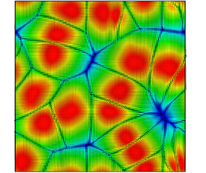
The above description implies that, once again, the relationship between the pattern and the multiplicity of heated elements sensitively depends on the horizontal extension of the elements (δhoriz) as further illustrated in the following. In particular, as shown in figure 14 for δhoriz = 1.0, the steady and very ordered distribution of small surface square cells for N = 5 (simply reflecting the underlying 5 × 5 matrix of elements periodically positioned on the bottom, figure 14a), is taken over for N = 7 (figure 14b) by an aesthetically appealing convective configuration with many ‘spokes’ (loci of points where the surface velocity undergoes a kind of ‘discontinuity’) and four large approximately square cells located in the corners of the domain; a complex internal circulation structure can be also seen where the surface fluid is driven towards a central sink (this being witnessed by the distribution of the surface velocity component along x in figure 14d).

Figure 14. Surface vector plot (a,b) and distribution of velocity component along x (c,d) for δhoriz = 1 and different values of N (mixed convection, adiabatic floor and adiabatic lateral solid walls): (a,c) N = 5 (steady flow); (b,d) N = 7 (unsteady flow).
This special point (knot) with fourfold topology corresponds to a kind of ‘singular’ vertex where the fluid (reaching it along different horizontal directions) is finally pushed towards the bottom of the layer. As yet visible in figure 14(b,d), all the other knots have a smaller topological order p = 3. The corresponding surface temperature distribution (reported in the third panel of the first row of figure 13) essentially consists of a single thermal loop formed by many plumes surrounding a central colder region that culminates in a central peak where the surface temperature attains its smallest possible value (this point occupies the same position of the aforementioned knot with topological order 4).
This flow is weakly time dependent. In particular, flow unsteadiness essentially stems from localized effects, which consist of a ‘flickering’ (back and forth) motion of the spokes along directions approximately perpendicular to them; more precisely, the overall time-dependent behaviour is characterized by two apparently disjoint temporal scales, one related to the just-mentioned localized oscillation of the spokes and another due to a more general process by which some cells undergo a slow adjustment in time. The latter results in minor changes in cell position and shape (we will come back to this aspect later; the reader being referred to the extended discussion reported in § 5).
These results obviously further support the realization that once a certain value of N is exceeded, these systems contain their own capacity for transformation, which can promote the emergence of planforms with well-defined (non-trivial) features.
Notably, when the system has entered the specific regime where the surface pattern is no longer a trivial (1 : 1) manifestation of the underlying topography, a switch in the thermal boundary condition at the bottom (from adiabatic to isothermal) has a weak impact. These observations are quantitatively substantiated by figure 15 (N = 7 and δhoriz = 1); apart from some minor modification (compare figure 15 with figure 14b,d), the flow has the same structure and topology (remarkably, we found the same pattern also by running a simulation with N = 9 and adiabatic floor, not shown).

Figure 15. Isosurfaces of vertical velocity component ((a), green = −3,2, red = 11.3) and surface vector plot (b) for the hot floor case (mixed convection, adiabatic lateral solid walls), N = 7 and δhoriz = 1 (unsteady flow,  $Nu_{side}^{average} \cong 0.329$, $Nu_{top}^{average} \cong 1.154$, $Nu_{bar}^{average} \cong 0.704$).
Vice versa, the variation is dramatic if the swap in the thermal boundary condition is implemented for systems which have not entered yet the self-organization regime, see figure 16 (N = 7 and δhoriz = 0.1). As implicitly revealed by this figure, in place of the trivial array of perfectly aligned spots which would be obtained for N = 7 with the adiabatic floor condition (figure 13, third row, third panel), a planform with well-defined properties is produced. Notably, it possesses all of the symmetries pertaining to the aforementioned D 4 group, i.e. the mirror reflections with respect to the vertical planes  $x = {A_{horiz}}/2$, $z = {A_{horiz}}/2$, x = z and $z = {A_{horiz}} - x$ and related combinations.

Figure 16. Isosurfaces of vertical velocity (green = −3,2, red = 11.3) component (a), surface vector plot (b) and temperature distribution in the xy midplane (c) for the hot floor case (mixed convection, adiabatic lateral solid walls), N = 7 and δhoriz = 0.1 (steady flow,  $Nu_{side}^{average} \cong 1.398$, $Nu_{top}^{average} \cong 8.525$, $Nu_{bar}^{average} \cong 1.947$).
In a quite unexpected way, in this case the topological order of the central knot is even increased with respect to the preceding cases (pmax = 8), while other knots do not exist at all. Figures 16(a) and 16(b) are naturally complemented by figure 16(c), where evidence is provided that the perfect symmetry of the flow (and the ensuing increase in the topological order of the central knot) is supported by a kind of synchronization between specific heated blocks and the location of the dominant thermal plumes. Apparently, specific blocks play the role of ‘catalysts’ in generating rising currents, thereby stabilizing the flow, which becomes essentially steady.
A further understanding of all these modes of convection can be gained by considering the related behaviour in terms of heat exchange between the hot elements and the fluid. Following the same approach implemented in § 4.1, we content ourselves with developing this subject solely for the situations with adiabatic floor and solid sidewalls for which the majority of the present results have been obtained (figure 17).

Figure 17. Nusselt number as a function of N for the configurations with adiabatic floor and adiabatic lateral solid walls (mixed convection, the splines are used to guide the eye): (a) δhoriz = 1; (b) δhoriz = 0.55; (c) δhoriz = 0.1.
Correlation of figures 17(a) and 8(a) (δhoriz = 1.0 cases) is instrumental in revealing that (as expected) the presence of an additional mechanism of convection located at the free surface causes an appreciable rise in the values of  $Nu_{top}^{average}$. Vice versa, no significant variations can be seen in $Nu_{side}^{average}$ both in terms of magnitude and trend (compare again figures 8a and 17a).
The increase in  $Nu_{top}^{average}$is still appreciable for smaller values of δhoriz. For δhoriz = 0.55 (figure 17b), $Nu_{top}^{average}$ is now located above the corresponding $Nu_{side}^{average}$ line as opposed to the situation seen in figure 8(b). For δhoriz = 0.1 (figure 17c) a big gap separates $Nu_{top}^{average}$ and $Nu_{side}^{average}$. Like the equivalent situation with only buoyancy flow (figure 8c), the reason for the proximity of $Nu_{bar}^{average}$ to $Nu_{side}^{average}$ resides in the fact that the top area of each element is very small with respect to its total lateral area (which, as made evident by (2.14) contributes to make $Nu_{bar}^{average} \cong Nu_{side}^{average}$).
4.3. Microgravity conditions
A separate discussion is needed for the Ra = 0 circumstances, the surface expression of which in the classical situation with uniform heating (and no topography) would be the canonical MB convection. It is worth recalling that, strictly speaking, this kind of flow can be obtained only in microgravity conditions (where the influence of buoyancy forces can be completely filtered out). In normal gravity, situations approaching those for which pure MB convection is obtained can be mimicked by reducing the ratio Ra/Ma as much as possible (typically by decreasing the depth of the considered layer), i.e. if Bodyn ≅ 0. The results presented in this section could therefore be applied in principle to experiment performed on an orbiting platform (such as the International Space Station) or on Earth in ‘microscale’ conditions (layer depth significantly smaller than 1 mm). This subject has received significant attention over the years (though not being comparable to that attracted by the companion problem represented by RB convection). Other studies worthy of mention in addition to those reported in the introduction and the book by Colinet et al. (Reference Colinet, Legros and Velarde2001) are those by Thess & Bestehron (Reference Thess and Bestehorn1995) and Bestehorn (Reference Bestehorn1996), who concentrated on the evolution of the emerging planforms, showing that the well-known hexagonal symmetry of the cells (underpinned by a threefold organization of the vertices, i.e. p = 3) is spontaneously taken over for larger values of Ma by a fourfold vertex topology (p = 4) resulting in square-shaped convective cells. Given the amount of literature available on this specific subject, these references are obviously selective samples of existing valuable investigations. However, studies concerned with the regime where this form of convection becomes disordered in both time and space are relatively rare (Thess & Orszag Reference Thess and Orszag1994, Reference Thess and Orszag1995; Thess, Spirn & Jiittner Reference Thess, Spirn and Jiittner1995, Reference Thess, Spirn and Jiittner1996); we will use them for some conclusive arguments elaborated in § 5. In the present section, we limit ourselves to describing the dynamics found in the present conditions by setting Ra = 0.
As shown by figure 18, in terms of symmetries, considerations very similar to those already developed in § 4.2 could be given. For the sake of brevity, we limit ourselves to re-emphasizing that the loss of symmetry with respect to the aforementioned D 4 group still manifest itself in conjunction with transition to time-dependent convection, which indicates that this should be seen as a bifurcation of the flow.

Figure 18. Combined view of surface temperature and velocity distribution for δhoriz = 1 and different values of N (microgravity conditions, adiabatic floor and adiabatic lateral solid walls): (a) N = 5 (steady flow); (b) N = 7 (unsteady flow).
Consideration of a representative hot floor case is also instructive (figure 19). Without buoyancy, the ability of the heated protuberances with small transverse extension (δhoriz) to exert an influence on the emerging pattern and its spatio-temporal behaviour is relatively limited. In place of the perfect (and steady) arrangement of cells observed in figure 16 for N = 7, δhoriz = 0.1 and Bodyn = 2, an unsteady pattern with four large thermal spots is obtained when Bodyn = 0 (figure 19).
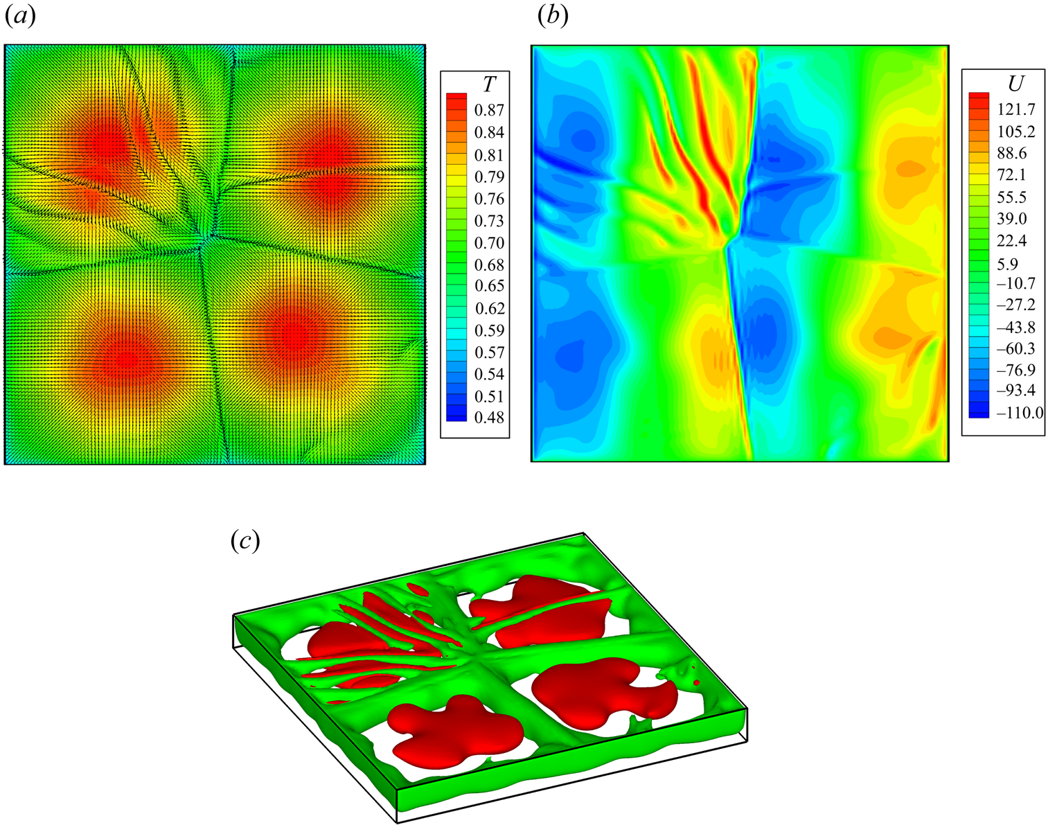
Figure 19. Combined view of surface temperature and velocity distribution (a); surface distribution of velocity component along x (b); isosurfaces of vertical velocity (green = −3,2, red = 9.2) component (c) for N = 7 and δhoriz = 0.1 (pure surface-tension-driven convection, hot floor and adiabatic lateral solid walls, unsteady flow with a localized oscillon,  $Nu_{side}^{average} \cong 1.578$, $Nu_{top}^{average} \cong 10.517$, $Nu_{bar}^{average} \cong 2.265$).
Continuing with a focused review of the literature on classical MB convection, we wish to remark that oscillatory behaviours relatively similar to that shown in figure 19 have also been observed in other studies dealing with classical MB convection. As an example, while investigating the possible existence of multiple solutions (states which depend on the initial conditions) for slightly supercritical conditions, Kvarving, Bjøntegaard & Rønquist (Reference Kvarving, Bjøntegaard and Rønquist2012) found that the final state of MB convection may be dominated by a steady convection pattern with a fixed number of cells, or the same system may occasionally end up in a steady pattern involving a slightly different number of cells, or it may display a peculiar convective configuration where most of the cells are stationary, while one or more cells undergo a localized oscillatory process (a cell being continuously destroyed and re-formed as time passes).
This is what can also be seen in figure 19, where the oscillations display a strongly confined nature. The affected cell does not disappear. Rather it apparently undergoes a localized instability, which results in a series of ripples originating from the central segment where the two cells aligned along the NorthWest–SouthEast (NW–SE) diagonal meet. All these spokes are embedded inside a single cell, while the rest of the pattern is seemingly not affected by them.
We also take these observations as a cue to recall another related concept, that is, the notion of the ‘oscillon’, already used in previous works. In Lappa & Ferialdi (Reference Lappa and Ferialdi2018), it was loosely defined as the spontaneous localization or confinement of oscillatory phenomena to a limited subregion of an otherwise stationary pattern in a translationally invariant system. Although the present system is no longer perfectly isotropic like the classical MB, the present results show that in the presence of a repetitive topography or thermal forcing, this definition or concept can still be considered relevant.
As a concluding remark for this section, in line with similar considerations elaborated for the companion circumstances with pure buoyancy or mixed buoyancy–Marangoni convection, we focus on the heat exchange behaviour. Along these lines, for the purpose of quantifying the variation undergone by such effects, figure 20 and table 4 show the related Nusselt number for various cases. The major outcome of figure 20 (through critical comparison with the equivalent figures 8a and 17a) resides in the indirect confirmation that most of the increase of  $Nu_{top}^{average}$ for δhoriz = 1 (adiabatic floor case) and relatively small values of N when surface-tension effects are added to buoyancy (by which $Nu_{top}^{average}$ becomes almost equal to $Nu_{side}^{average}$), essentially stems from the Marangoni effect itself.

Figure 20. Nusselt number as a function of N for the configurations with pure surface-tension-driven convection, δhoriz = 1, adiabatic floor and adiabatic lateral solid walls (the splines are used to guide the eye).
Table 4. Comparison between the Nusselt number obtained for configurations with hot bottom wall in different circumstances (N = 7, δhoriz = 0.1).

5. Discussion
5.1. The strongly nonlinear regime of MB flow
A critical discussion of earlier studies in companion fields (and related theoretical outcomes) is used in this section to elaborate some additional arguments for the interpretation of the observed dynamics.
In particular, as a first level of this specific abstraction hierarchy, we consider the main outcomes of the existing literature where models were specifically introduced to characterize chaos in MB systems. More specifically we refer to the line of inquiry originating from the studies by Thess & Orszag (Reference Thess and Orszag1994, Reference Thess and Orszag1995), where the so-called ‘strongly nonlinear regime’ of MB flow was examined (enabled when the Marangoni number based on the temperature difference between the bottom wall and the free surface exceeds a value of 2000). These authors studied this problem under the assumption of infinite value of the Prandtl number (because it leads to convenient simplifications in the governing equations) and revealed that the dynamics typical of this regime has a ‘signature’ that makes it very peculiar even when it is compared with akin phenomena such as turbulence in buoyancy flow (i.e. notable differences also exist with regard to the ‘hard RB turbulence’ originally analysed by Castaing et al. Reference Castaing, Gunaratne, Heslot, Kadanoff, Libchaber, Thomae, Wu, Zaleski and Zanetti1989).
As assumed by this model, MB flows in high-Pr fluids are dominated by viscous effects, while the temperature isolines become strongly deformed. Moreover, it considers the thermal diffusivity everywhere negligible with the exception of thin thermal layers. Earlier simulations based on such approach have shown that the temperature field consists of parabolic regions separated by increasingly sharp transition layers at the cell boundary, where the temperature gradient experiences a discontinuity (as an example, Thess & Orszag (Reference Thess and Orszag1994, Reference Thess and Orszag1995) could reveal such discontinuities through evaluation of the second derivative of the surface temperature).
The existence of such discontinuities also led researchers to naturally identify an analogy with the slow dynamics of the Burgers equation; in this regard, we wish to recall that the specific mathematical properties of this equation are known to produce shock discontinuities (as shown by figures 14–16, 18 and 19, such discontinuities also manifest in the present results, where they appear in the form of spokes emanating from specific points).
Some variants have also been elaborated where in place of an infinite Prandtl number, investigators focused on the  $Ma \to \infty$ idealized asymptotic state. Also this condition was found to be advantageous because in this limit the thickness of the surface Marangoni layer tends to zero, thereby allowing for 2-D models to be developed. Notably, in such a theoretical/mathematical context, Thess et al. (Reference Thess, Spirn and Jiittner1995, Reference Thess, Spirn and Jiittner1996) and Colinet et al. (Reference Colinet, Legros and Velarde2001) could reduce the original 3-D problem to a 2-D nonlinear evolution equation involving only free surface quantities ‘under the perspective that any statistical quantity related to the three-dimensional velocity field could be considered a function of the two-dimensional surface temperature only’.
The most important outcome of all this focused theoretical effort resides in the connection that has been established between the formation of the discontinuities of the temperature gradient (that emerge in a random way causing the splitting of large convective cells into smaller ones) and the instability of the surface thermal boundary-layer.
The present results obtained through solution of the original equations in their complete form essentially demonstrate that these concepts are also applicable to situations where the Prandtl number takes a finite value. The discontinuities manifest as spokes in the velocity field, corresponding to the presence of ripples in the temperature distribution, which, in turn, are produced as a result of instability of the surface temperature boundary layer. The adherence of the present results to this interpretation is further witnessed by the peculiar scaling (in terms of wavenumbers) displayed by the surface temperature distribution, which in these cases (as we will show in § 5.3) follows the same universal spectrum  $E(k) \propto {k^{ - 3}}$ predicted by Thess et al. (Reference Thess, Spirn and Jiittner1995, Reference Thess, Spirn and Jiittner1996) and Colinet et al. (Reference Colinet, Legros and Velarde2001).
Notably, in our case the spatial surface spectrum of temperature aligns very well with that predicted by such models not only in the circumstances where flow is produced by surface tension alone, but also in the cases where buoyancy is significant (which leads to the conclusion that for Bodyn = 2 and Bodyn = 0, the (spatial) scaling properties of the surface turbulence are essentially the same).
5.2. Quantized states and buoyancy effects
Although comparison with other existing numerical simulations for high values of Ma conducted in the limit as the Prandtl number tends to infinite or assuming an infinite value of the Marangoni number (boundary-layer model) shows that the related dynamics is in good agreement with that depicted in §§ 4.2 and 4.3, however, it should not be forgotten that the present problem is different, in the sense that while in some circumstances ‘quantized’ states are produced (i.e. ‘typical’ solutions where the pattern becomes independent from the properties of the bottom), in other cases non-trivial states emerge which do depend on the underlying morphologically and thermally textured wall (i.e. the size and spacing of the blocks).
The present dynamics is made more complex or intriguing by the existence of what we have called the self-organization regime. Again comparison with the literature can help to shed some additional light on such a scenario. In this regard, it is certainly worth considering the earlier experimental investigation by Ismagilov et al. (Reference Ismagilov, Rosmarin, Gracias, Stroock and Whitesides2001).
As outlined in the introduction, by means of infrared imaging, Ismagilov et al. (Reference Ismagilov, Rosmarin, Gracias, Stroock and Whitesides2001) revealed that when the convective cells typical of MB convection form under the same conditions that would produce ‘standard’ MB convection, but over a periodically patterned surface (uniformly heated), a specific kind of complexity is produced that is not possible when the bottom wall is perfectly planar and with no corrugations. More precisely, they found a kind of competition between the ‘intrinsic spatial periodicity’ of the flow (i.e. the wavelength of the planform that would be produced in the absence of topography) and the geometrical properties of the considered wall. This was found to result in a non-smooth (jerky) behaviour consisting of a set of discrete states, i.e. the ability of the fluid system to undergo abrupt transitions between different planforms (commensurate with the imposed shape of the bottom boundary) as the ratio of the intrinsic (wavelength) and perturbing length scales (size and morphology of the bulges) was changed.
This trend is consistent with what we have observed in the present study (where the same pattern has been found for different conditions, figures 14b,d and 15). Here, however, the patterned nature of the bottom wall has not been limited to the presence of bulges (the cubic elements in our case). Some control on the flow has also been exerted through the related thermal properties (i.e. through thermal forcing). Assuming the portion of floor between adjoining elements to be adiabatic, we have observed that new types of planforms can be produced which reflect neither the ordered distribution of elements at the bottom (through a trivial 1 : 1 correspondence), nor states which would be typical of standard MB convection.
In this regard, comparison of mixed buoyancy/Marangoni (§ 4.2) and pure MB flow (§ 4.3) has proved effective in allowing discerning the role played by buoyancy in such processes. This adds new information to the study by Ismagilov et al. (Reference Ismagilov, Rosmarin, Gracias, Stroock and Whitesides2001) where, owing the small thickness of the layer (100 cSt silicone oil with depth ≅0.8 mm), buoyancy was almost negligible  $(B{o_{dyn}} = \rho g{\beta _T}{d^2}/{\sigma _T} \cong 0.1)$. Another important difference concerns the degree of supercriticality. In Ismagilov et al. (Reference Ismagilov, Rosmarin, Gracias, Stroock and Whitesides2001) circumstances were considered for which the emerging planform of standard MB convection would correspond to the classical pattern with the honeycomb symmetry. Here, conditions enabling the so-called ‘strongly nonlinear dynamics’, originally examined by Thess & Orszag (Reference Thess and Orszag1994, Reference Thess and Orszag1995), have been investigated.
As widely illustrated in §§ 4.1 and 4.2, for Ma = 5 × 10³ and Bodyn = 2, buoyancy enhances the role of thermal forcing through the generation of warm plumes that originate from the top surface of the heated elements. This effect can contribute to make the emerging solutions and related pattern more regular than the corresponding flow in the absence of buoyancy. As a result, buoyancy can also strengthen the system abilities to produce new patterns (e.g. the one shown in figure 16).
5.3. Temporal scaling laws and confinement effects
This final subsection is dedicated to an aspect that has been glossed over until now, namely, the influence of the lateral confinement (the sidewalls, which, as already shown in earlier valuable fundamental studies, can play a non-negligible role in the dynamics of Marangoni–Rayleigh–Bénard convection, see, e.g. Dauby & Lebon Reference Dauby and Lebon1996; Medale & Cerisier Reference Medale and Cerisier2002).
In order to implement such discussion and obtain some statistically meaningful data (i.e. insights which display a sufficiently high level of generality), we consider two representative cases, all pertaining to the sub-region of the space of parameters where non-trivial patterns emerge. These are the configuration with adiabatic boundary (N = 7, δhoriz = 1) and the one with isothermal floor (N = 7, δhoriz = 0.1). The analysis is developed considering the temporal evolution of the Nusselt numbers  $Nu_{side}^{average}$ and $Nu_{top}^{average}$ and velocity signals (velocity component along the horizontal direction u as a function of time) provided by numerical probes located above the heated blocks (at an intermediate position between the top of the block and the free surface of the layer). In particular, the Nusselt number is characterized in terms of frequency spectrum, that is, a further understanding of the observed phenomena is gained by considering a fine-grained micromechanical perspective able to provide information on the small spatial scales of the flow. We explicitly use such a strategy to uncover features that could not be revealed by the macrophysical approach (based only on the spatial properties of the patterns) developed in § 4.
Simulations conducted replacing the solid vertical boundaries with PBC have confirmed that the lateral confinement contributes significantly to the perfection of some of the stable and highly ordered structures reported in §§ 4.2 and 4.3.
As a first example of this influence, figure 21(a,b) (N = 7, δhoriz = 1, adiabatic floor, see also supplementary movie 1 available at https://doi.org/10.1017/jfm.2022.175) immediately reveals that, if the no-slip lateral walls are replaced by PBC, the pattern takes a relatively disordered spatio-temporal organization with respect to that obtained under confinement (reported for the convenience of the reader in figure 21c). The well-defined ring of hot spots (cell) surrounding a central knot with topological order p = 4 (clearly visible in figure 21c) can no longer be recognized in figure 21(a). In place of a structure dominated by p = 3 knots (and a single central p = 4 point), a much more complex network of spokes is produced, with cells having a number of sides ranging between 3 and 6 (from triangles to irregular hexagons) and knots with topological order much larger than that seen for the configuration with solid walls (increasing up to p = 9 as witnessed by the presence of one or more flower-like structures with many petals).

Figure 21. Mixed convection for N = 7, δhoriz = 1 and adiabatic floor: (a) combined view of surface temperature and velocity distribution for the case with periodic lateral boundary conditions (four snapshots equally spaced in time, Δτ = 1.0); (b) related surface temperature spectrum (line x = 3.55 at t ≅ 6); (c) combined view of surface temperature and velocity distribution for the case with solid sidewalls (snapshot at t = 5.25).
On a separate note, it is also worth highlighting the trend displayed by the related surface temperature (spatial) spectrum (figure 21b). It follows essentially the same k −3 scaling predicted by the models for highly supercritical MB convection discussed in § 5.1.
The next figure of the sequence (figure 22) refers to the aforementioned case where the floor is not adiabatic (hot bottom wall). As the reader will easily realize by inspecting it (see also supplementary movie 2), in such a situation, the changes induced by a swap in the lateral boundary conditions are even more dramatic. While the flow arising with solid sidewalls was essentially steady (figure 22c), when PBC are applied, this is taken over by completely different spatial and temporal convective mechanism. The p = 8 multiplicity of the central knot is lost (a central knot even does no longer exist or make sense). The cross-shaped network formed by cell boundaries (figure 22c) is replaced by a much more complex topology (figure 22a). An interesting (peculiar) behaviour can be seen where the fluid is pushed down (blue regions). These are characterized by the presence of some ripples.

Figure 22. Mixed convection for N = 7, δhoriz = 0.1 and hot floor: (a) combined view of surface temperature and velocity distribution for the case with periodic lateral boundary conditions (four snapshots equally spaced in time, Δτ = 1.0); (b) surface temperature spectrum (line x = 3.52 at t = 6); (c) combined view of surface temperature and velocity distribution for the case with solid sidewalls (snapshot at t = 3.44).
Notably, the surface temperature distribution (figure 22b) still obeys the k −3 scaling found for the other cases.
We wish to remark that, besides the spatial scaling law for the surface temperature spectrum (distribution of wavenumbers), all these cases with PBC also share another remarkable property, which needs to be pinpointed suitably here. Although, thermal ripples leading to localized splitting of cells are present in almost all cases (just like for the cases with solid sidewalls), the most significant contribution to time dependence now comes from the continuous modification in the size, shape and positions of the cells.
Unlike the discretely heated configurations under lateral confinement shown in figure 21(c), where time dependence occasionally manifests as defects that travel slowly in the pattern along the horizontal direction or localized ‘vibrating’ spokes that cause breaking of cells into two or more parts, with PBC, the temporal behaviour consists of cells that, ‘like boats drifting in open water’, continuously wander in an endless process. This peculiar motion, which closely resembles that found by Lappa & Ferialdi (Reference Lappa and Ferialdi2018) for slightly supercritical MB convection in viscoelastic fluids, affects the entire physical domain (figures 21a and 22a). The characteristic time with which cells move is smaller than the equivalent one corresponding to the slow re-adjustment process occurring in the presence of sidewalls. This observation is qualitatively and quantitatively substantiated by the velocity signals reported in figures 23(a) and 23(b) for the case N = 7, δhoriz = 1 and adiabatic floor.

Figure 23. Signals provided by probes located above the heated blocks (y = 0.65) for N = 7, δhoriz = 1.0 and adiabatic floor: (a) solid lateral walls (mixed convection); (b) PBC (mixed convection), (c) solid lateral walls in microgravity conditions (Ra = 0), (d) PBC in microgravity conditions (Ra = 0).
Following up on the previous point, these two panels immediately show that the simple (slow) adjustment of the cells on a relatively long time scale (figure 23a) for solid sidewalls is taken over for PBC by a faster process made visible by the increased number of valleys and mountains in the velocity signals (figure 23b). Localized (high- frequency) oscillations superimposed on an otherwise smaller-frequency signal are present in both cases. Obviously, these correspond to the flickering of spokes repeatedly discussed before, which exists independently of the motion of cells. Most remarkably, the vibrating spokes are the dominant source of unsteadiness when pure Marangoni flow limited by sidewalls is considered (the sinusoidal distortions visible in figure 23(c) have a very limited amplitude). The last figure of the sequence (figure 23d) naturally complements the earlier observations by making evident that, even in the absence of buoyancy, pure Marangoni flow with PBC can yet display a progressive cell repositioning mechanism. It is also worth noting that the amplitude of the oscillations related to the vibrating spokes increases as the solid walls are replaced with PBCs regardless of whether gravity is present or not.
To elucidate further the significance and implications of these findings, figure 24 finally reports the amplitudes of the different modes that contribute to the frequency spectrum of the element Nusselt numbers for the flows with both buoyancy and Marangoni effects. It can be seen that the continuous and relatively fast cell wandering allowed by the lack of sidewalls leads to a ω −3/2 dependence visible in the high-frequency range of the spectrum regardless of the thermal condition assumed for the bottom wall,  $\omega$ is the angular frequency.

Figure 24. Frequency spectrum for the Nusselt number (mixed convection, PBC at the lateral boundaries): (a) adiabatic floor, N = 7, δhoriz = 1; (b) hot floor, N = 7 and δhoriz = 0.1 [ $Nu_{side}^{average}$ (black line), $Nu_{top}^{average}$ (red line), related scaling law (blue line)].
6. Conclusions
We have investigated the peculiar dynamics that a morphological alteration (topography) of the bottom wall consisting of periodically positioned cubic (hot) blocks can induce in an overlying layer of a high-Pr liquid (Pr = 10) with an upper free surface.
In articulating this problem, our specific aim was to move beyond the idealized limitations of the classical RB and MB paradigms, which so much attention have attracted over several decades in terms of hierarchy of bifurcations and patterning behaviour (up to the onset of chaos). In order to identify the correspondence between the geometrical and thermal characteristics of the bottom wall and the emerging flow in terms of textural, temporal and heat exchange properties, a systematic effort has been provided to map the complexity of such conditions into a corresponding zoo of patterns.
Given the intrinsic nature of thermal convection induced by gravity, surface tension or both driving forces, fulfilling such objective has required a fully 3-D approach based on the integration of the nonlinear and time-dependent governing equations.
Taking advantage of this framework, we have observed that the connection between the flow structure and the underlying structure is not as straightforward as one would imagine since a variety of factors can contribute to determine the related nonlinear feedback or coupling mechanisms. The relationship between a patterned boundary (intended as repetition of sudden variations in its shape and related thermal attributes) and the flow field induced accordingly is just like the interrelation between two fundamental types of properties of any system in nature: characteristics that appear as a consequence of the interaction of the system with its environment (the larger system of which it is a part) through all its ‘boundaries’ and features that emerge as a result of mechanisms inherent within the system itself (its sensitivity to certain categories of fluid-dynamic disturbances).
Put together these aspects determine how the behaviour of the considered system arises from detailed structures and interdependencies on a smaller scale. In particular, three distinct regimes, have been identified for the situation considered in the present work: trivial modes of convection where the surface pattern simply reflects (through a 1 : 1 correspondence) the ordered distribution of the underlying hot elements, states that display a notable degree of analogy with the ‘parent’ convective mechanisms (classical RB and/or MB flow) and a third category of flows represented by possible solutions driven by intrinsic self-organization abilities of the considered system (enabled when a given threshold in terms of number or horizontal size of the elements is exceeded).
Although such a general classification has been found to hold for all the considered combinations of characteristic numbers (Ra ≠ 0, Ma = 0), (Ra = 0, Ma ≠ 0) and (Ra ≠ 0, Ma ≠ 0), significant differences have been observed depending on the involved driving forces. For pure buoyancy convection, transition from trivial patterns to more complex ones is essentially driven by thermal plume interaction mechanisms. Such processes result in shrinkage of the dimension of the matrix that can be used to map the distribution of surface spots in comparison with the size of the underlying grid of hot elements. For Ra = 104, only steady solutions exist. With the addition of surface-tension effects (Bodyn = 2), the complexity of the problem increases as unsteadiness enters the dynamics and points (vertices) with relatively high topological order pop up in the spatial network of surface spokes. These ‘knots’ behave as the centres of closed polygonal multi-cellular structures. Due to their existence, in general, the flow can be considered more ordered (both in time and space) than the corresponding convective state that would be obtained assuming a flat and isothermal floor (Marangoni–Rayleigh–Bénard flow).
Although surface-tension effects become dominant, buoyancy does still play a role in such phenomena. This has been revealed through direct comparison of microgravity and terrestrial conditions, leading to the realization that the hot blocks evenly spaced along the bottom can contribute to the regularity of the flow spatial organization through the creation of thermal pillars at fixed positions (still able to influence accordingly surface flow).
The involved driving forces, however, are not the only influential factor driving the outcomes of the fluid-bottom-wall interaction. This process is also mediated by apparently secondary details such as the thermal behaviour of the portion of floor between adjoining elements and (especially) the kinematic condition at the system side (its outer rim).
If the adiabatic bottom wall (on which the hot blocks are placed) is replaced with an isothermal floor (at the same temperature as the blocks) and the distribution of elements is dilute and/or their horizontal extension is small, the intrinsic mechanisms of the parent forms (MB, RB) of convection obviously tend to become dominant in determining the emerging planform. However, this is not a general rule, as in some cases the separated elements can still serve as ‘catalysts’ for the formation of well-defined and stable plumes.
Replacement of the solid lateral wall with PBC has even more significant consequences, especially in terms of temporal dynamics. The triadic relationship between the hierarchy of involved driving forces, the lateral confinement and the system temporal response can be summarized as follows. For pure Marangoni convection (microgravity conditions) and solid lateral walls, unsteadiness essentially manifests itself in the form of high-frequency oscillations physically corresponding to the existence of vibrating spokes in the pattern, which cause localized cell breaking or coalescence effects. If buoyancy is also present, these high-frequency modes are complemented by long-period disturbances corresponding to the slow propagation of defects through the pattern (a slow displacement of the cell centres occurring on time scale comparable to the thermal diffusion time). For PBC, this slow process is taken over by a different phenomenon by which cells undergo a faster relocation in time, accompanied by significant changes in their size and shape.
In order to interpret this kaleidoscope of possible variants, a concerted approach has been implemented using the tools of computational fluid dynamics in synergy with existing models on the evolution of MB convection for highly supercritical Ma. Interestingly, we have shown that the pattern of surface temperature is forced to follow the k −3 spatial scaling originally identified by other authors (Thess and co-workers) regardless of the amplitude of buoyancy flow for Bodyn up to 2.
The present study has been conducted under the optimistic hope that this theoretical framework and its combination with numerical simulations will open up the way for a new line of inquiry to rationally connect the properties of canonical forms of convection (well-established paradigms) to the more intricate situations represented by the many practical realizations one has to deal with in several fields (the reader being referred again to the extended descriptions provided in the introduction). Along these lines, we think that future studies shall be devoted to expanding the dimensionality of the space of parameters examined here, e.g. by considering larger values of the dynamic Bond number and eventually changing parametrically the vertical extension of the hot blocks.
Supplemental movies
Supplementary movies are available at https://doi.org/10.1017/jfm.2022.175.
Acknowledgements
The authors would like to thank A. Boaro for the calculation of the data reported in figures 21, 22 and 24.
Declaration of interests
The authors report no conflict of interest.


 Open access