


1. Introduction
The boundary conditions between a mushy layer (a reactive porous medium) and a liquid melt involve a complex interaction between thermodynamics and fluid flow (Beckermann & Wang Reference Beckermann, Wang and Tien1995; Schulze & Worster Reference Schulze and Worster1999, Reference Schulze and Worster2005). A mushy layer comprising dendritic crystals and residual melt often forms when a two-component mixture solidifies. Pressure gradients, buoyancy gradients, external shear and internal phase change can all drive fluid flows through the porous medium. Boundaries between a mushy and a liquid region are a vital part of any description of a mushy layer. For example, at the wall of a dissolution channel in a solidifying convecting mushy layer (Copley et al. Reference Copley, Giamei, Johnson and Hornbecker1970), there is an outflow into the channel, and appropriate boundary conditions are needed to determine the size of the channel. For this situation, motivated by the idea that a mushy layer grows to relieve supercooling of the liquid, Schulze & Worster (Reference Schulze and Worster1999, Reference Schulze and Worster2005) derived a condition of marginal equilibrium, which requires that streamlines are tangent to isotherms at the boundary.
In this paper, we investigate a potential inconsistency of marginal equilibrium associated with a slip in the tangential velocity at a mush–liquid interface (Beavers & Joseph Reference Beavers and Joseph1967). We use the idea of a transition region inside the mushy layer that has a width of a few pore lengths where we apply the Stokes equation for viscous flow, following Le Bars & Worster (Reference Le Bars and Worster2006). This allows us to investigate the effect of slip in the tangential velocity within a two-domain formulation of mushy-layer theory, while retaining a continuous velocity on the microscale, which is necessary for marginal equilibrium. We do not intend the transition region to constitute a complete description of the fluid flow near the interface. However, it is a self-consistent alternative to using the Darcy–Brinkman equation to describe the flow in both the mushy layer and the liquid region. These alternatives were shown by Le Bars & Worster (Reference Le Bars and Worster2006) to give comparable results for a transition region of prescribed dimensionless width
 $$\begin{eqnarray}{\it\delta}=c\mathscr{D}^{1/2},\quad \text{where}\;c=O(1),\,\mathscr{D}={\it\Pi}_{0}/H^{2},\end{eqnarray}$$
and the dimensionless Darcy number
 $\mathscr{D}$
is the ratio of a characteristic permeability
$\mathscr{D}$
is the ratio of a characteristic permeability
 ${\it\Pi}_{0}$
to the square of a length scale
${\it\Pi}_{0}$
to the square of a length scale
 $H$
characteristic of the width of the mushy layer.
$H$
characteristic of the width of the mushy layer.
In §§ 2 and 3 respectively we present interior equations and boundary conditions for an ideal mushy layer (Worster Reference Worster1997, Reference Worster, Batchelor, Moffatt and Worster2000; Schulze & Worster Reference Schulze and Worster2005). In § 4, we apply these equations to a simple ‘toy’ problem with a two-dimensional corner flow, using a configuration originally formulated by Conroy & Worster (Reference Conroy and Worster2006) and Le Bars & Worster (Reference Le Bars and Worster2006), because the marginal equilibrium condition at an outflow boundary is fundamentally two-dimensional. In § 5 we present semi-analytical results that explain the regions of parameter space in which there is a steady mush–liquid interface, and we discuss these results in § 6.
2. Mushy-layer and liquid-region equations
We work with the equations for an ideal mushy layer describing conservation of mass, heat, solute and momentum, as well as a liquidus relationship between temperature
 $T$
and interstitial (or liquid-region) concentration
$T$
and interstitial (or liquid-region) concentration
 $C$
,
$C$
,
 $$\begin{eqnarray}\displaystyle & \displaystyle \boldsymbol{{\rm\nabla}}\boldsymbol{\cdot }\boldsymbol{q}=0, & \displaystyle\end{eqnarray}$$
 $$\begin{eqnarray}\displaystyle & \displaystyle \frac{\text{D}T}{\text{D}t}={\it\kappa}{\rm\nabla}^{2}T+\frac{L}{c_{p}}\frac{\text{D}^{s}{\it\phi}}{\text{D}t}, & \displaystyle\end{eqnarray}$$
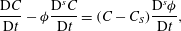 $$\begin{eqnarray}\displaystyle & \displaystyle \frac{\text{D}C}{\text{D}t}-{\it\phi}\frac{\text{D}^{s}C}{\text{D}t}=(C-C_{S})\frac{\text{D}^{s}{\it\phi}}{\text{D}t}, & \displaystyle\end{eqnarray}$$
 $$\begin{eqnarray}\displaystyle & \displaystyle {\it\mu}\boldsymbol{u}=-{\it\Pi}\boldsymbol{{\rm\nabla}}p, & \displaystyle\end{eqnarray}$$
 $$\begin{eqnarray}\displaystyle & \displaystyle T=T_{L}(C)\equiv T_{m}-m(C-C_{S}), & \displaystyle\end{eqnarray}$$
 ${\it\phi}$
is the volume fraction occupied by the solid phase. We use the material derivatives
${\it\phi}$
is the volume fraction occupied by the solid phase. We use the material derivatives
 $\text{D}^{s}/\text{D}t$
moving with the solid phase of velocity
$\text{D}^{s}/\text{D}t$
moving with the solid phase of velocity
 $\boldsymbol{v}$
, and
$\boldsymbol{v}$
, and
 $\text{D}/\text{D}t$
moving with the total flux
$\text{D}/\text{D}t$
moving with the total flux
 $\boldsymbol{q}=\boldsymbol{u}+\boldsymbol{v}$
, where
$\boldsymbol{q}=\boldsymbol{u}+\boldsymbol{v}$
, where
 $\boldsymbol{u}$
is the Darcy velocity. In the idealization, it is assumed that the phases have the same material and thermal properties (particularly latent heat of solidification
$\boldsymbol{u}$
is the Darcy velocity. In the idealization, it is assumed that the phases have the same material and thermal properties (particularly latent heat of solidification
 $L$
and heat capacity
$L$
and heat capacity
 $c_{p}$
) and that the liquidus is linear with gradient
$c_{p}$
) and that the liquidus is linear with gradient
 $-m$
. The concentration of the solid phase
$-m$
. The concentration of the solid phase
 $C_{S}=0$
and the melting temperature is
$C_{S}=0$
and the melting temperature is
 $T_{m}$
. The solute diffusivity, which is much less than the thermal diffusivity
$T_{m}$
. The solute diffusivity, which is much less than the thermal diffusivity
 ${\it\kappa}$
, is neglected. The permeability of the porous medium is
${\it\kappa}$
, is neglected. The permeability of the porous medium is
 ${\it\Pi}$
and the dynamic viscosity of the fluid is
${\it\Pi}$
and the dynamic viscosity of the fluid is
 ${\it\mu}$
. The flow is driven by the pressure gradient
${\it\mu}$
. The flow is driven by the pressure gradient
 $\boldsymbol{{\rm\nabla}}p$
and we neglect buoyancy-driven flow.
$\boldsymbol{{\rm\nabla}}p$
and we neglect buoyancy-driven flow.
Equations (2.1)–(2.3) hold in the liquid region where
 $\boldsymbol{q}$
is the fluid velocity and
$\boldsymbol{q}$
is the fluid velocity and
 ${\it\phi}=0$
. In the liquid region, fluid flow is governed by the Stokes equation
${\it\phi}=0$
. In the liquid region, fluid flow is governed by the Stokes equation
 $$\begin{eqnarray}{\it\mu}{\rm\nabla}^{2}\boldsymbol{q}=\boldsymbol{{\rm\nabla}}p.\end{eqnarray}$$
Neglect of solute diffusion in the liquid region implies that the concentration is constant along streamlines there, which is an important consideration in the development of the interfacial conditions between mush and liquid (Schulze & Worster Reference Schulze and Worster1999).
An important feature of the model is that there is a transition region between the mushy layer and the liquid region in which the solid fraction is non-zero and the thermodynamics is described by the mushy-layer equations while the flow is described by the Stokes equation.
3. Mushy-layer boundary conditions
At a mush–liquid interface, we apply continuity of temperature and heat flux,
 $$\begin{eqnarray}[T]_{l}^{m}=0,\quad VL{\it\phi}_{m}=c_{p}{\it\kappa}[\boldsymbol{n}\boldsymbol{\cdot }\boldsymbol{{\rm\nabla}}T]_{l}^{m},\end{eqnarray}$$
where
 $V$
is the velocity of the interface relative to the solid phase in the direction
$V$
is the velocity of the interface relative to the solid phase in the direction
 $\boldsymbol{n}$
, a unit vector normal to the interface (from mush to liquid) and the subscripts
$\boldsymbol{n}$
, a unit vector normal to the interface (from mush to liquid) and the subscripts
 $m$
and
$m$
and
 $l$
denote quantities evaluated on the mush and liquid sides of the interface respectively. Solute conservation across the interface implies that
$l$
denote quantities evaluated on the mush and liquid sides of the interface respectively. Solute conservation across the interface implies that
 $$\begin{eqnarray}-[C]_{l}^{m}U={\it\phi}_{m}(C_{m}-C_{S})V,\end{eqnarray}$$
where
 $U$
is the velocity of the liquid phase relative to the mush–liquid interface. Thus if, as in the case of outflow,
$U$
is the velocity of the liquid phase relative to the mush–liquid interface. Thus if, as in the case of outflow,
 $[C]_{l}^{m}=0$
(the concentration is continuous), then
$[C]_{l}^{m}=0$
(the concentration is continuous), then
 ${\it\phi}_{m}=0$
at the interface, and vice versa.
${\it\phi}_{m}=0$
at the interface, and vice versa.
Schulze & Worster (Reference Schulze and Worster1999, Reference Schulze and Worster2005) showed that the conditions of heat and salt conservation are insufficient to determine the location of the interface for a solidifying mushy layer,
 $V>0$
. Therefore, motivated by the fact that a mushy layer grows to alleviate constitutional supercooling, they derived a condition of marginal equilibrium. For inflow,
$V>0$
. Therefore, motivated by the fact that a mushy layer grows to alleviate constitutional supercooling, they derived a condition of marginal equilibrium. For inflow,
 $U<0$
, the marginal equilibrium condition extends the liquidus condition (2.5) into the liquid such that the temperature satisfies
$U<0$
, the marginal equilibrium condition extends the liquidus condition (2.5) into the liquid such that the temperature satisfies
 $\boldsymbol{n}\boldsymbol{\cdot }\boldsymbol{{\rm\nabla}}T_{l}=\boldsymbol{n}\boldsymbol{\cdot }\boldsymbol{{\rm\nabla}}T_{L}(C_{l})$
, as originally proposed by Worster (Reference Worster1986). For outflow,
$\boldsymbol{n}\boldsymbol{\cdot }\boldsymbol{{\rm\nabla}}T_{l}=\boldsymbol{n}\boldsymbol{\cdot }\boldsymbol{{\rm\nabla}}T_{L}(C_{l})$
, as originally proposed by Worster (Reference Worster1986). For outflow,
 $U>0$
, the marginal equilibrium condition requires that
$U>0$
, the marginal equilibrium condition requires that
 $$\begin{eqnarray}\frac{\text{D}T}{\text{D}t}=0.\end{eqnarray}$$
4. Solidification with a corner flow
4.1. Problem formulation
We consider a semi-infinite rectangular channel of width
 $H$
in a directional solidification configuration (with the pulling speed
$H$
in a directional solidification configuration (with the pulling speed
 $V$
in the negative
$V$
in the negative
 $z$
-direction, which is equivalent to a solidification rate
$z$
-direction, which is equivalent to a solidification rate
 $V$
). This configuration permits steady solutions in which the mush–liquid interface is fixed, the solid phase has velocity
$V$
). This configuration permits steady solutions in which the mush–liquid interface is fixed, the solid phase has velocity
 $\boldsymbol{v}=-V\hat{\boldsymbol{z}}$
, and corresponds to the experimental apparatus of Peppin et al. (Reference Peppin, Aussillous, Huppert and Worster2007). We impose boundary temperatures
$\boldsymbol{v}=-V\hat{\boldsymbol{z}}$
, and corresponds to the experimental apparatus of Peppin et al. (Reference Peppin, Aussillous, Huppert and Worster2007). We impose boundary temperatures
 $T=T_{m}-(k_{1,2}/H)x,0<x<\infty$
, on two permeable walls, where
$T=T_{m}-(k_{1,2}/H)x,0<x<\infty$
, on two permeable walls, where
 $x$
is the distance along the channel. We choose the constants
$x$
is the distance along the channel. We choose the constants
 $k_{1}$
and
$k_{1}$
and
 $k_{2}$
with
$k_{2}$
with
 $k_{1}>k_{2}$
such that the lower wall, which is adjacent to a mushy layer, is colder than the upper wall, which is adjacent to a liquid melt that occupies a fraction
$k_{1}>k_{2}$
such that the lower wall, which is adjacent to a mushy layer, is colder than the upper wall, which is adjacent to a liquid melt that occupies a fraction
 $1-{\it\eta}$
of the channel, as shown in figure 1(a). To control the flow, we impose the total normal flux
$1-{\it\eta}$
of the channel, as shown in figure 1(a). To control the flow, we impose the total normal flux
 $\boldsymbol{q}\boldsymbol{\cdot }\boldsymbol{e}_{z}=Q_{1,2}$
at the permeable walls, where
$\boldsymbol{q}\boldsymbol{\cdot }\boldsymbol{e}_{z}=Q_{1,2}$
at the permeable walls, where
 $\boldsymbol{e}_{z}$
is a unit vector in the
$\boldsymbol{e}_{z}$
is a unit vector in the
 $z$
direction. We also impose no slip
$z$
direction. We also impose no slip
 $\boldsymbol{u}\boldsymbol{\cdot }\boldsymbol{e}_{x}=0$
at the upper wall in the figure, where
$\boldsymbol{u}\boldsymbol{\cdot }\boldsymbol{e}_{x}=0$
at the upper wall in the figure, where
 $\boldsymbol{e}_{x}$
is a unit vector in the
$\boldsymbol{e}_{x}$
is a unit vector in the
 $x$
direction.
$x$
direction.


Figure 1(b) shows the dimensionless version of this problem. We non-dimensionalize lengths with respect to the dimensional channel width
 $H$
and velocities with respect to
$H$
and velocities with respect to
 $Q_{1}$
. Henceforth,
$Q_{1}$
. Henceforth,
 $x$
and
$x$
and
 $z$
denote dimensionless lengths. The ratio of imposed fluxes
$z$
denote dimensionless lengths. The ratio of imposed fluxes
 $r=Q_{2}/Q_{1}$
determines the direction of the flow, with
$r=Q_{2}/Q_{1}$
determines the direction of the flow, with
 $r<1$
corresponding to flow towards the positive
$r<1$
corresponding to flow towards the positive
 $x$
-direction. We restrict attention to the case
$x$
-direction. We restrict attention to the case
 $r>0$
to ensure outflow.
$r>0$
to ensure outflow.
We seek a self-similar solution in which the dimensionless temperature and interstitial concentration can be written in the form
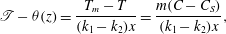 $$\begin{eqnarray}\mathscr{T}-{\it\theta}(z)=\frac{T_{m}-T}{(k_{1}-k_{2})x}=\frac{m(C-C_{S})}{(k_{1}-k_{2})x},\end{eqnarray}$$
where
 $\mathscr{T}=k_{2}/(k_{1}-k_{2})>{\it\theta}$
gives a measure of the ratio of horizontal to vertical temperature gradients at the upper boundary.
$\mathscr{T}=k_{2}/(k_{1}-k_{2})>{\it\theta}$
gives a measure of the ratio of horizontal to vertical temperature gradients at the upper boundary.
Motivated by the separable solution for Stokes flow in a corner (Batchelor Reference Batchelor1967), we seek a corresponding similarity solution for the dimensionless material flux in the form
 $$\begin{eqnarray}\boldsymbol{q}/Q_{1}=[-xf^{\prime }(z),f(z)],\end{eqnarray}$$
cf. Le Bars & Worster (Reference Le Bars and Worster2006). This mathematical framework allows for a two-dimensional flow to be analysed conveniently with one-dimensional equations in
 $z$
. We note that this similarity solution is consistent with symmetry boundary conditions on the flow at
$z$
. We note that this similarity solution is consistent with symmetry boundary conditions on the flow at
 $x=0$
, and
$x=0$
, and
 $T(0,z)=T_{m}$
.
$T(0,z)=T_{m}$
.
4.2. Dimensionless fluid flow
In the liquid and transition regions, the flow satisfies the dimensionless Stokes equation
 ${\rm\nabla}^{2}\boldsymbol{q}=\boldsymbol{{\rm\nabla}}p$
. Eliminating the pressure, we find that the Stokes equation becomes
${\rm\nabla}^{2}\boldsymbol{q}=\boldsymbol{{\rm\nabla}}p$
. Eliminating the pressure, we find that the Stokes equation becomes
 $f^{(4)}(z)=0$
. In the mushy layer, the flow satisfies Darcy’s law (2.4), which becomes
$f^{(4)}(z)=0$
. In the mushy layer, the flow satisfies Darcy’s law (2.4), which becomes
 $(\,f^{\prime }/{\it\Pi})^{\prime }=0$
. In the simplest case of uniform permeability
$(\,f^{\prime }/{\it\Pi})^{\prime }=0$
. In the simplest case of uniform permeability
 ${\it\Pi}={\it\Pi}_{0}$
, the solution that satisfies the boundary conditions at
${\it\Pi}={\it\Pi}_{0}$
, the solution that satisfies the boundary conditions at
 $z=0$
and
$z=0$
and
 $z=1$
is
$z=1$
is
 $$\begin{eqnarray}\displaystyle & f=C_{0}z+1,\quad 0\leqslant z\leqslant {\it\eta}-{\it\delta}, & \displaystyle\end{eqnarray}$$
 $$\begin{eqnarray}\displaystyle & f=B_{0}(1-z)^{3}+A_{0}(1-z)^{2}+r,\quad {\it\eta}-{\it\delta}\leqslant z\leqslant 1, & \displaystyle\end{eqnarray}$$
 $A_{0}$
,
$A_{0}$
,
 $B_{0}$
and
$B_{0}$
and
 $C_{0}$
are constants that can be derived from mass conservation, no slip and continuity of pressure at the boundary between Stokes and Darcy flow,
$C_{0}$
are constants that can be derived from mass conservation, no slip and continuity of pressure at the boundary between Stokes and Darcy flow,  $$\begin{eqnarray}[\,f]=0,\quad [\,f^{\prime }]=0,\quad \left.f^{\prime \prime \prime }\right|^{+}=-\left.f^{\prime }\right|^{-}/\mathscr{D}\qquad (z={\it\eta}-{\it\delta}),\end{eqnarray}$$
respectively. We find that
 $$\begin{eqnarray}A_{0}=-3B_{0}\left[\frac{{\it\gamma}}{2}+\frac{\mathscr{D}}{{\it\gamma}}\right],\quad B_{0}=\frac{2(r-1)}{{\it\gamma}^{3}+6\mathscr{D}(2-{\it\gamma})},\quad C_{0}=6\mathscr{D}B_{0},\end{eqnarray}$$
where
 ${\it\gamma}=1-{\it\eta}+{\it\delta}$
. Note that the streamfunction
${\it\gamma}=1-{\it\eta}+{\it\delta}$
. Note that the streamfunction
 $f$
is continuously differentiable (although its second derivative is not continuous and we use superscripts in (4.5c
) to denote the relevant side of the Stokes–Darcy boundary). Therefore, there are well defined streamlines at the mush–liquid interface, essential to both deriving and also imposing the marginal equilibrium condition (Schulze & Worster Reference Schulze and Worster2005). We now solve the thermodynamic part of the problem.
$f$
is continuously differentiable (although its second derivative is not continuous and we use superscripts in (4.5c
) to denote the relevant side of the Stokes–Darcy boundary). Therefore, there are well defined streamlines at the mush–liquid interface, essential to both deriving and also imposing the marginal equilibrium condition (Schulze & Worster Reference Schulze and Worster2005). We now solve the thermodynamic part of the problem.
4.3. Dimensionless interior equations
The ideal mushy-layer equations (2.2), (2.3) in the case of steady directional solidification give
 $$\begin{eqnarray}\displaystyle f{\it\theta}^{\prime }-f^{\prime }({\it\theta}-\mathscr{T})={\it\theta}^{\prime \prime }/Pe-\mathscr{S}\mathscr{V }{\it\phi}^{\prime }, & \ 0\leqslant z\leqslant {\it\eta}, & \displaystyle\end{eqnarray}$$
 $$\begin{eqnarray}\displaystyle f{\it\theta}^{\prime }-f^{\prime }({\it\theta}-\mathscr{T})=-\mathscr{V }[{\it\phi}({\it\theta}-\mathscr{T})]^{\prime }, & \ 0\leqslant z\leqslant {\it\eta}, & \displaystyle\end{eqnarray}$$
 $\mathscr{V }=V/Q_{1}$
represents the ratio of the solidification rate to the imposed flow and
$\mathscr{V }=V/Q_{1}$
represents the ratio of the solidification rate to the imposed flow and
 $Pe=Q_{1}H/{\it\kappa}$
is a Péclet number representing the ratio of advection by the imposed flow to diffusion of heat. The Stefan number
$Pe=Q_{1}H/{\it\kappa}$
is a Péclet number representing the ratio of advection by the imposed flow to diffusion of heat. The Stefan number
 $\mathscr{S}=L/(c_{p}(k_{1}-k_{2})x)$
, so we can neglect latent heat release at sufficiently large
$\mathscr{S}=L/(c_{p}(k_{1}-k_{2})x)$
, so we can neglect latent heat release at sufficiently large
 $x$
where
$x$
where
 $\mathscr{S}\ll 1$
.
$\mathscr{S}\ll 1$
.
Equation (4.7) with
 ${\it\phi}=0$
is also the heat equation for the liquid region
${\it\phi}=0$
is also the heat equation for the liquid region
 ${\it\eta}\leqslant z\leqslant 1$
. Salt conservation in the liquid region is governed by
${\it\eta}\leqslant z\leqslant 1$
. Salt conservation in the liquid region is governed by
 $\boldsymbol{q}\boldsymbol{\cdot }\boldsymbol{{\rm\nabla}}C=0$
, so
$\boldsymbol{q}\boldsymbol{\cdot }\boldsymbol{{\rm\nabla}}C=0$
, so
 $C\propto xf(z)$
.
$C\propto xf(z)$
.
4.4. Dimensionless boundary conditions
The dimensionless boundary conditions on temperature are
 $$\begin{eqnarray}{\it\theta}(0)=-1,\quad {\it\theta}(1)=0,\quad [{\it\theta}]_{l}^{m}=0,\quad [{\it\theta}^{\prime }]_{l}^{m}=0,\end{eqnarray}$$
provided
 $\mathscr{S}\ll 1$
so that latent heat release at the interface is insignificant.
$\mathscr{S}\ll 1$
so that latent heat release at the interface is insignificant.
For solidifying outflow (
 $V,U>0$
), conservation of solute (3.2) and marginal equilibrium (3.3) require that
$V,U>0$
), conservation of solute (3.2) and marginal equilibrium (3.3) require that
 $$\begin{eqnarray}\displaystyle & [C]_{m}^{l}=0\Rightarrow {\it\phi}_{m}=0, & \displaystyle\end{eqnarray}$$
 $$\begin{eqnarray}\displaystyle & \boldsymbol{q}\boldsymbol{\cdot }\boldsymbol{{\rm\nabla}}{\it\theta}=0\Rightarrow f{\it\theta}^{\prime }-f^{\prime }({\it\theta}-\mathscr{T})=0\quad (z={\it\eta}). & \displaystyle\end{eqnarray}$$
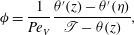
In general, we solve these equations numerically, iterating such that (4.11) is satisfied. We find the first integral of (4.8) analytically, using (4.7), to determine
 $$\begin{eqnarray}{\it\phi}=\frac{1}{Pe_{V}}\frac{{\it\theta}^{\prime }-{\it\theta}({\it\eta})}{\mathscr{T}-{\it\theta}},\qquad 0\leqslant z\leqslant {\it\eta},\end{eqnarray}$$
where
 $Pe_{V}=VH/{\it\kappa}=\mathscr{V }Pe$
is a Péclet number based on the solidification rate. Thus the solid fraction is inversely proportional to the solidification rate
$Pe_{V}=VH/{\it\kappa}=\mathscr{V }Pe$
is a Péclet number based on the solidification rate. Thus the solid fraction is inversely proportional to the solidification rate
 $V$
. Figure 2 shows a typical example of a solution. Note that marginal equilibrium is satisfied, so streamlines are tangential to isotherms at the mush–liquid interface.
$V$
. Figure 2 shows a typical example of a solution. Note that marginal equilibrium is satisfied, so streamlines are tangential to isotherms at the mush–liquid interface.
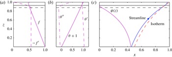
Figure 2. A typical solution for the dimensionless variables (magenta curves, labelled). The transition region between the dashed horizontal line and the solid horizontal line at the mush–liquid interface has width
 ${\it\delta}=0.05$
(
${\it\delta}=0.05$
(
 $c=0.5,\mathscr{D}=0.01$
). Other parameters are
$c=0.5,\mathscr{D}=0.01$
). Other parameters are
 $r=0.47,Pe=\mathscr{T}=1$
. (a) Flow function
$r=0.47,Pe=\mathscr{T}=1$
. (a) Flow function
 $f$
and the negative of its derivative, proportional to the vertical and horizontal velocities respectively. (b) Temperature
$f$
and the negative of its derivative, proportional to the vertical and horizontal velocities respectively. (b) Temperature
 ${\it\theta}$
and its derivatives. It should be noted that
${\it\theta}$
and its derivatives. It should be noted that
 ${\it\theta}^{\prime \prime }$
becomes increasingly negative in the mushy layer and only starts to increase in the transition region, and
${\it\theta}^{\prime \prime }$
becomes increasingly negative in the mushy layer and only starts to increase in the transition region, and
 ${\it\theta}^{\prime \prime }({\it\eta})=0$
. (c) The solid fraction
${\it\theta}^{\prime \prime }({\it\eta})=0$
. (c) The solid fraction
 ${\it\phi}$
, which increases away from the interface, and an illustration of the marginal equilibrium condition: a streamline (blue, direction of flow indicated by an arrow) and an isotherm (red, dashed) are tangential at the mush–liquid interface.
${\it\phi}$
, which increases away from the interface, and an illustration of the marginal equilibrium condition: a streamline (blue, direction of flow indicated by an arrow) and an isotherm (red, dashed) are tangential at the mush–liquid interface.
5. Results in the case of a solidifying mushy layer with outflow
Steady solutions only exist in a limited region of parameter space (figure 3) because of two crucial constraints. (I) If the outflow
 $Q_{2}$
becomes too strong relative to the inflow
$Q_{2}$
becomes too strong relative to the inflow
 $Q_{1}$
, the isotherms become convex, which is inconsistent with the twin requirements of marginal equilibrium and a positive solid fraction, as shown in sketch A in figure 3. Physically, the mushy layer is dissolved away as there is not enough advection from the cold lower boundary. An important implication of this first constraint is that there are no solutions without a transition region. (II) If
$Q_{1}$
, the isotherms become convex, which is inconsistent with the twin requirements of marginal equilibrium and a positive solid fraction, as shown in sketch A in figure 3. Physically, the mushy layer is dissolved away as there is not enough advection from the cold lower boundary. An important implication of this first constraint is that there are no solutions without a transition region. (II) If
 $Q_{2}$
is too weak, the direction of the temperature gradient at the upper wall reverses, which is inconsistent with marginal equilibrium, as shown in sketch C in figure 3. Physically, the mushy layer advances and the width of the liquid region goes to zero.
$Q_{2}$
is too weak, the direction of the temperature gradient at the upper wall reverses, which is inconsistent with marginal equilibrium, as shown in sketch C in figure 3. Physically, the mushy layer advances and the width of the liquid region goes to zero.
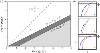
Figure 3. A regime diagram showing the dependence on the imposed flow. In region A, there are no steady solutions because the solid fraction is negative. This region is divided into two by the dashed line
 $r=1$
(
$r=1$
(
 $Q_{2}=Q_{1}$
), which separates flow to the left from flow to the right. In region B, there is a unique steady solution. The width of the liquid region decreases towards region C, in which there are no steady solutions because the mushy layer occupies the whole channel. The boundaries are labelled (I) and (II) and are discussed in §§ 5.1 and 5.2 respectively. Figure 3(b) shows sketched streamlines (blue, direction of flow indicated with an arrow) and isotherms (dashed, red) and a vertical arrow showing the retreat (A), steady state (B) or advance (C) of the mush–liquid interface. The regime diagram is in the physically meaningful limit of small Darcy number
$Q_{2}=Q_{1}$
), which separates flow to the left from flow to the right. In region B, there is a unique steady solution. The width of the liquid region decreases towards region C, in which there are no steady solutions because the mushy layer occupies the whole channel. The boundaries are labelled (I) and (II) and are discussed in §§ 5.1 and 5.2 respectively. Figure 3(b) shows sketched streamlines (blue, direction of flow indicated with an arrow) and isotherms (dashed, red) and a vertical arrow showing the retreat (A), steady state (B) or advance (C) of the mush–liquid interface. The regime diagram is in the physically meaningful limit of small Darcy number
 $\mathscr{D}\rightarrow 0$
,
$\mathscr{D}\rightarrow 0$
,
 $\mathscr{T}=1$
, and it is independent of
$\mathscr{T}=1$
, and it is independent of
 $c>0$
. Thus, the regime diagram does not depend on the absolute size of the transition region, provided it is non-zero.
$c>0$
. Thus, the regime diagram does not depend on the absolute size of the transition region, provided it is non-zero.
5.1. The concavity of isotherms (I)
We take the asymptotic limit Darcy number
 $\mathscr{D}\rightarrow 0$
, in which both the transition region and the liquid region are narrow (see § 5.3). Mathematically, it is required to prove that
$\mathscr{D}\rightarrow 0$
, in which both the transition region and the liquid region are narrow (see § 5.3). Mathematically, it is required to prove that
 ${\it\theta}^{\prime \prime }(z)<0$
in the mushy layer given that
${\it\theta}^{\prime \prime }(z)<0$
in the mushy layer given that
 ${\it\phi}>0$
. Informally, the argument is that (2.3) implies that
${\it\phi}>0$
. Informally, the argument is that (2.3) implies that
 $\text{D}C/\text{D}t>0$
, since all the terms on the right-hand side are positive, at least sufficiently close to the mush–liquid interface. Then, the liquidus condition (2.5) shows that
$\text{D}C/\text{D}t>0$
, since all the terms on the right-hand side are positive, at least sufficiently close to the mush–liquid interface. Then, the liquidus condition (2.5) shows that
 $\text{D}T/\text{D}t<0$
, whence
$\text{D}T/\text{D}t<0$
, whence
 ${\rm\nabla}^{2}T<0$
using (2.2), as required. More formally, we differentiate (4.7) with respect to
${\rm\nabla}^{2}T<0$
using (2.2), as required. More formally, we differentiate (4.7) with respect to
 $z$
to find
$z$
to find
 $$\begin{eqnarray}{\it\theta}^{\prime \prime \prime }/Pe=f{\it\theta}^{\prime \prime }-f^{\prime \prime }({\it\theta}-\mathscr{T}).\end{eqnarray}$$
In the mushy layer (excluding the narrow transition zone),
 $f^{\prime \prime }=0$
and
$f^{\prime \prime }=0$
and
 $f>0$
, so
$f>0$
, so
 ${\it\theta}^{\prime \prime }$
has a definite sign. However, in the transition zone,
${\it\theta}^{\prime \prime }$
has a definite sign. However, in the transition zone,
 $f^{\prime \prime }\neq 0$
and
$f^{\prime \prime }\neq 0$
and
 ${\it\theta}^{\prime \prime }$
changes rapidly (as
${\it\theta}^{\prime \prime }$
changes rapidly (as
 $\mathscr{D}^{-1/2}$
) to satisfy
$\mathscr{D}^{-1/2}$
) to satisfy
 ${\it\theta}^{\prime \prime }({\it\eta})=0$
(cf. figure 2
b). Given that
${\it\theta}^{\prime \prime }({\it\eta})=0$
(cf. figure 2
b). Given that
 ${\it\phi}({\it\eta})=0$
,
${\it\phi}({\it\eta})=0$
,
 ${\it\phi}$
must increase as
${\it\phi}$
must increase as
 $z$
decreases away from the interface
$z$
decreases away from the interface
 $z={\it\eta}$
. From (4.7), (4.8), this requires
$z={\it\eta}$
. From (4.7), (4.8), this requires
 ${\it\theta}^{\prime \prime }({\it\eta}^{-})<0$
, so
${\it\theta}^{\prime \prime }({\it\eta}^{-})<0$
, so
 ${\it\theta}^{\prime \prime }(z)<0$
, as claimed.
${\it\theta}^{\prime \prime }(z)<0$
, as claimed.
The physical reason why the transition region is crucial can also be inferred from (5.1). In the mushy layer, the horizontal velocity is uniform. However, in the transition region it decreases rapidly, cf. figures 2(a,c). This decrease allows horizontal and vertical advection of heat to balance at the mush–liquid interface, as required by the marginal equilibrium condition (4.11). (Note that only the horizontal velocity changes across the transition region to leading order as
 $\mathscr{D}\rightarrow 0$
.)
$\mathscr{D}\rightarrow 0$
.)
Furthermore, our asymptotic analysis shows that
 $f,f^{\prime },{\it\theta},{\it\theta}^{\prime }$
and
$f,f^{\prime },{\it\theta},{\it\theta}^{\prime }$
and
 ${\it\theta}^{\prime \prime }$
are all
${\it\theta}^{\prime \prime }$
are all
 $O(1)$
in the Darcy number, so the full solution for
$O(1)$
in the Darcy number, so the full solution for
 ${\it\theta}$
and
${\it\theta}$
and
 ${\it\theta}^{\prime }$
can be found to leading order in the Darcy number by solving (4.7) with the linear flow function
${\it\theta}^{\prime }$
can be found to leading order in the Darcy number by solving (4.7) with the linear flow function
 $f(z)=1+C_{0}z$
because the mush occupies almost all of the domain. Now,
$f(z)=1+C_{0}z$
because the mush occupies almost all of the domain. Now,
 $C_{0}\sim (r-1)$
from (4.6a−c
). For notational simplicity, we introduce a depth-dependent Péclet number
$C_{0}\sim (r-1)$
from (4.6a−c
). For notational simplicity, we introduce a depth-dependent Péclet number
 $P(z)=Pe[1-z(1-r)]$
and difference
$P(z)=Pe[1-z(1-r)]$
and difference
 ${\rm\Delta}P=Pe(1-r)$
. Then, we find the exact solution for the temperature field
${\rm\Delta}P=Pe(1-r)$
. Then, we find the exact solution for the temperature field
 $$\begin{eqnarray}{\it\theta}(z)=\mathscr{T}+K_{1}P+K_{2}\left[\sqrt{\frac{{\rm\pi}}{2{\rm\Delta}P}}P\,\text{erf}\left(\frac{P}{\sqrt{2{\rm\Delta}P}}\right)+\exp \left(\frac{-P^{2}}{2{\rm\Delta}P}\right)\right],\end{eqnarray}$$
where
 $K_{1}$
and
$K_{1}$
and
 $K_{2}$
are constants determined by the boundary conditions
$K_{2}$
are constants determined by the boundary conditions
 ${\it\theta}(0)=-1$
and
${\it\theta}(0)=-1$
and
 ${\it\theta}(1)=0$
. Thus, there is a unique solution that satisfies the boundary conditions, except in the singular one-dimensional case of
${\it\theta}(1)=0$
. Thus, there is a unique solution that satisfies the boundary conditions, except in the singular one-dimensional case of
 ${\rm\Delta}P=0$
. Note that (5.2) holds if
${\rm\Delta}P=0$
. Note that (5.2) holds if
 ${\rm\Delta}P<0$
, and gives real solutions.
${\rm\Delta}P<0$
, and gives real solutions.
We determine the boundary (I) in figure 3 by considering the marginal case
 ${\it\theta}^{\prime \prime }(z)=0$
, which occurs if and only if
${\it\theta}^{\prime \prime }(z)=0$
, which occurs if and only if
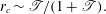
 $$\begin{eqnarray}r=\mathscr{T}/(1+\mathscr{T}).\end{eqnarray}$$
A consequence is that
 $r<1$
(greater inflow than outflow, meaning that flow is from left to right and so from fresher to saltier).
$r<1$
(greater inflow than outflow, meaning that flow is from left to right and so from fresher to saltier).
5.2. The heat flux from the upper heat exchanger is positive (II)
The marginal equilibrium condition (4.11) requires that the horizontal advection of warm fluid from the left is balanced by the vertical advection of cold fluid from below. Thus, there are no steady solutions unless
 ${\it\theta}^{\prime }(1)>0$
.
${\it\theta}^{\prime }(1)>0$
.
We determine the boundary (II) in figure 3 by considering the marginal case
 ${\it\theta}^{\prime }(1)=0$
. To fix ideas, we consider the natural special case of no flux through the upper wall,
${\it\theta}^{\prime }(1)=0$
. To fix ideas, we consider the natural special case of no flux through the upper wall,
 $r=0$
. There is a critical
$r=0$
. There is a critical
 $\mathscr{T}=\mathscr{T}_{C}$
, above which there are no solutions, where
$\mathscr{T}=\mathscr{T}_{C}$
, above which there are no solutions, where
 $$\begin{eqnarray}\mathscr{T}_{C}=[\sqrt{{\rm\pi}Pe/2}\;\text{erf}(\sqrt{Pe/2})+\exp (-Pe/2)-1]^{-1}.\end{eqnarray}$$
The inverse of this relationship gives a critical
 $Pe_{C}(\mathscr{T})$
(i.e. input flux
$Pe_{C}(\mathscr{T})$
(i.e. input flux
 $Q_{1}$
). Note that
$Q_{1}$
). Note that
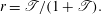
 $\mathscr{T}_{C}\sim 2/Pe$
as
$\mathscr{T}_{C}\sim 2/Pe$
as
 $Pe\rightarrow 0$
and
$Pe\rightarrow 0$
and
 $\mathscr{T}_{C}\sim \sqrt{2/{\rm\pi}Pe}$
as
$\mathscr{T}_{C}\sim \sqrt{2/{\rm\pi}Pe}$
as
 $Pe\rightarrow \infty$
, as shown in figure 4(a).
$Pe\rightarrow \infty$
, as shown in figure 4(a).
Figure 4. (a) The critical temperature gradient ratio
 $\mathscr{T}_{C}$
in the special case
$\mathscr{T}_{C}$
in the special case
 $r=0$
. The dashed lines give the asymptotic scalings described in the main text. (b) The critical ratio of outflow to inflow
$r=0$
. The dashed lines give the asymptotic scalings described in the main text. (b) The critical ratio of outflow to inflow
 $r_{c}$
, above which there are steady solutions, for three given values of
$r_{c}$
, above which there are steady solutions, for three given values of
 $\mathscr{T}$
. It should be noted that the
$\mathscr{T}$
. It should be noted that the
 $r_{c}=0$
intercept is the critical
$r_{c}=0$
intercept is the critical
 $Pe_{C}$
in (a). The solid black squares denote the asymptotic value
$Pe_{C}$
in (a). The solid black squares denote the asymptotic value
 $r_{c}\sim \mathscr{T}/(1+\mathscr{T})$
(5.6). Note that, for small
$r_{c}\sim \mathscr{T}/(1+\mathscr{T})$
(5.6). Note that, for small
 $\mathscr{T}$
, the ratio at
$\mathscr{T}$
, the ratio at
 $Pe=20$
is much less than the asymptotic value, indicating a wide region of solutions.
$Pe=20$
is much less than the asymptotic value, indicating a wide region of solutions.
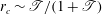
More generally, we find the boundary (II) – defined by, say,
 $r=r_{c}(Pe,\mathscr{T})$
– that satisfies a transcendental equation
$r=r_{c}(Pe,\mathscr{T})$
– that satisfies a transcendental equation
 $$\begin{eqnarray}\displaystyle & & \displaystyle (1+\mathscr{T})\exp \left(-\frac{r_{c}Pe^{2}}{2{\rm\Delta}P}\right)-\mathscr{T}\exp \left(-\frac{Pe^{2}}{2{\rm\Delta}P}\right)\nonumber\\ \displaystyle & & \displaystyle \quad =\mathscr{T}\sqrt{\frac{{\rm\pi}}{2{\rm\Delta}P}}Pe\left[\text{erf}\left(\frac{Pe}{\sqrt{2{\rm\Delta}P}}\right)-\text{erf}\left(\frac{r_{c}Pe}{\sqrt{2{\rm\Delta}P}}\right)\right].\end{eqnarray}$$
It is not difficult to show that this equation has a solution for all
 $Pe>Pe_{C}$
, which we plot in figure 4(b), and that, asymptotically for large
$Pe>Pe_{C}$
, which we plot in figure 4(b), and that, asymptotically for large
 $Pe$
,
$Pe$
,
 $$\begin{eqnarray}r_{c}\sim \mathscr{T}/(1+\mathscr{T}).\end{eqnarray}$$
This ratio also defines the top of region B. Thus, the region of parameter space where solutions exist becomes asymptotically narrow for large
 $Pe$
. However, if
$Pe$
. However, if
 $\mathscr{T}$
is small, there is a relatively wide region of solutions for a given
$\mathscr{T}$
is small, there is a relatively wide region of solutions for a given
 $Pe$
. Thus, if the horizontal temperature gradient is weak compared with the vertical gradient near the interface, marginal equilibrium is a much weaker constraint, because a smaller change in horizontal velocity is required to balance the horizontal and vertical transport of heat near the interface.
$Pe$
. Thus, if the horizontal temperature gradient is weak compared with the vertical gradient near the interface, marginal equilibrium is a much weaker constraint, because a smaller change in horizontal velocity is required to balance the horizontal and vertical transport of heat near the interface.
5.3. Liquid channel width and the necessity of a transition region
We now find a scaling for the liquid channel width in this configuration. Marginal equilibrium (4.11) gives
 $$\begin{eqnarray}-f^{\prime }({\it\eta})=f({\it\eta}){\it\theta}^{\prime }({\it\eta})/(\mathscr{T}-{\it\theta}({\it\eta}))\sim r{\it\theta}^{\prime }(1)/\mathscr{T}.\end{eqnarray}$$
Note that
 ${\it\theta}^{\prime }(1)$
is a function of
${\it\theta}^{\prime }(1)$
is a function of
 $(r,\mathscr{T},Pe)$
that can be determined from (5.2). Now, the conditions on the flow (4.5a−c
) give scalings
$(r,\mathscr{T},Pe)$
that can be determined from (5.2). Now, the conditions on the flow (4.5a−c
) give scalings
 $$\begin{eqnarray}f_{+}^{\prime \prime \prime }=f_{-}^{\prime }/\mathscr{D}\sim f_{+}^{\prime }/\mathscr{D}\quad (z={\it\eta}-{\it\delta}),\end{eqnarray}$$
where the subscript
 $+$
denotes the quantity on the transition zone side of the mush–transition zone interface and the subscript
$+$
denotes the quantity on the transition zone side of the mush–transition zone interface and the subscript
 $-$
the mush side. These scalings combine to give a liquid-region width
$-$
the mush side. These scalings combine to give a liquid-region width
 $$\begin{eqnarray}1-{\it\eta}\sim a_{0}\mathscr{D}^{1/2}.\end{eqnarray}$$
An alternative way to interpret this is to note that (5.1) implies that
 $f^{\prime \prime }({\it\eta})\sim {\it\delta}^{-1}\sim \mathscr{D}^{-1/2}$
, so the liquid-region width must scale with
$f^{\prime \prime }({\it\eta})\sim {\it\delta}^{-1}\sim \mathscr{D}^{-1/2}$
, so the liquid-region width must scale with
 $\mathscr{D}^{1/2}$
to balance viscous shear stresses. We determine the prefactor
$\mathscr{D}^{1/2}$
to balance viscous shear stresses. We determine the prefactor
 $a_{0}$
from the asymptotic solution for the flow
$a_{0}$
from the asymptotic solution for the flow
 $f(z)$
and (5.7). These yield the quadratic equation for
$f(z)$
and (5.7). These yield the quadratic equation for
 $a_{0}$
,
$a_{0}$
,
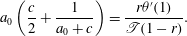 $$\begin{eqnarray}a_{0}\left(\frac{c}{2}+\frac{1}{a_{0}+c}\right)=\frac{r{\it\theta}^{\prime }(1)}{\mathscr{T}(1-r)}.\end{eqnarray}$$
For any finite
 $c>0$
, this equation has exactly one positive solution
$c>0$
, this equation has exactly one positive solution
 $a_{0}$
. However, for
$a_{0}$
. However, for
 $c=0$
there are no solutions (
$c=0$
there are no solutions (
 $c\rightarrow 0$
is a singular limit). Therefore, the transition region is crucial for the existence of steady solutions to the problem.
$c\rightarrow 0$
is a singular limit). Therefore, the transition region is crucial for the existence of steady solutions to the problem.
5.4. Solid fraction
Since
 ${\it\theta}^{\prime \prime }<0$
in the mushy layer,
${\it\theta}^{\prime \prime }<0$
in the mushy layer,
 ${\it\phi}>0$
. Furthermore, (4.12) shows that
${\it\phi}>0$
. Furthermore, (4.12) shows that
 $$\begin{eqnarray}{\it\phi}=\frac{1}{Pe_{V}}\frac{{\it\theta}^{\prime }(z)-{\it\theta}^{\prime }({\it\eta})}{\mathscr{T}-{\it\theta}(z)},\end{eqnarray}$$
so
 ${\it\phi}$
increases as
${\it\phi}$
increases as
 $z$
decreases away from the mush–liquid interface. The physical requirement that
$z$
decreases away from the mush–liquid interface. The physical requirement that
 ${\it\phi}\leqslant 1$
gives a critical
${\it\phi}\leqslant 1$
gives a critical
 $Pe_{V}$
(or solidification rate
$Pe_{V}$
(or solidification rate
 $V$
) above which solutions are physically meaningful. One important feature of the case of solidifying outflow is that both the size of the solid fraction in the mushy layer and also the concentration in the liquid region are determined everywhere by heat and salt conservation, and not by any imposed external boundary condition on
$V$
) above which solutions are physically meaningful. One important feature of the case of solidifying outflow is that both the size of the solid fraction in the mushy layer and also the concentration in the liquid region are determined everywhere by heat and salt conservation, and not by any imposed external boundary condition on
 ${\it\phi}$
. By contrast, in the case of a dissolving mushy layer, it is appropriate to impose
${\it\phi}$
. By contrast, in the case of a dissolving mushy layer, it is appropriate to impose
 ${\it\phi}$
at the lower heat exchanger.
${\it\phi}$
at the lower heat exchanger.
6. Discussion
The thermodynamic marginal equilibrium condition determines the position of the interface between a solidifying mushy layer and a purely liquid region when there is a fluid flow from the mush to the liquid. A potential difficulty with this condition arises in cases where a slip in the tangential velocity occurs at the interface. We have shown that extension of the Stokes equations into the mushy layer in a transition region whose width scales with
 $\mathscr{D}^{1/2}$
is a viable way to resolve this difficulty. This avoids relying on a single-domain approach with a fluid dynamical equation (such as Darcy–Brinkman) applying in both the liquid and the mushy layer, and shows that marginal equilibrium is a robust boundary condition.
$\mathscr{D}^{1/2}$
is a viable way to resolve this difficulty. This avoids relying on a single-domain approach with a fluid dynamical equation (such as Darcy–Brinkman) applying in both the liquid and the mushy layer, and shows that marginal equilibrium is a robust boundary condition.
By considering the simple ‘toy’ problem of solidification with a corner flow, we have understood several important features of flow in a mushy layer using simple physical and geometrical arguments, as well as asymptotic analysis. For our external boundary conditions on the flow, the transition region is strictly necessary for the existence of steady solutions. The need for a transition region is physically associated with the need for a rapid change in the component of the velocity tangential to the mush–liquid interface. Similarly, the vertical velocity increases rapidly in what we call the active region near a vertical chimney in a mushy layer with convection due to baroclinic torque (Rees Jones & Worster Reference Rees Jones and Worster2013). This is another way to explain why a finite active region near the chimney is needed to sustain mushy-layer convection. In our particular pressure-driven flow configuration, the widths of the liquid region and the transition region both scale with
 $\mathscr{D}^{1/2}$
(which dimensionally is a few pore lengths), which is somewhat problematic within the formal continuum limit. Nevertheless, the physical mechanisms that give rise to the regime diagram (figure 3) still apply at moderate values of
$\mathscr{D}^{1/2}$
(which dimensionally is a few pore lengths), which is somewhat problematic within the formal continuum limit. Nevertheless, the physical mechanisms that give rise to the regime diagram (figure 3) still apply at moderate values of
 $\mathscr{D}$
, and the diagram itself is independent of the prefactor
$\mathscr{D}$
, and the diagram itself is independent of the prefactor
 $c$
in the width of the transition region.
$c$
in the width of the transition region.
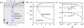
Figure 5. (a) Shear-driven flow with temperature gradient from cold to warm as
 $x$
and
$x$
and
 $z$
increase. (b) Typical isotherm (red dashed) and streamline (blue with arrows) for the same parameters as figure 2. Note the much wider liquid region. (c) Asymptotic scalings (dashed lines) for the width of the liquid region, verifying the first (squares) and second (circles) terms in equation (6.1) for
$z$
increase. (b) Typical isotherm (red dashed) and streamline (blue with arrows) for the same parameters as figure 2. Note the much wider liquid region. (c) Asymptotic scalings (dashed lines) for the width of the liquid region, verifying the first (squares) and second (circles) terms in equation (6.1) for
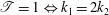 $\mathscr{T}=1\Leftrightarrow k_{1}=2k_{2}$
and
$\mathscr{T}=1\Leftrightarrow k_{1}=2k_{2}$
and
 $c=1$
.
$c=1$
.
Furthermore, there are other configurations in which the liquid region is asymptotically large compared with the transition region. By way of example, we briefly consider a shear-driven flow. If we reverse the overall temperature gradient and impose a viscous shear at the top of the liquid region that increases linearly with
 $x$
, the flow circulation that ensures positive solid fraction has the opposite configuration to the main pressure-driven flow part of this paper, as shown in figure 5. It should be noted that the equation of salt conservation cannot formally be treated in the similarity framework because far along the channel the local temperature would be above the liquidus. Using similar asymptotic techniques to § 5.1, we find that the liquid-region width is given by
$x$
, the flow circulation that ensures positive solid fraction has the opposite configuration to the main pressure-driven flow part of this paper, as shown in figure 5. It should be noted that the equation of salt conservation cannot formally be treated in the similarity framework because far along the channel the local temperature would be above the liquidus. Using similar asymptotic techniques to § 5.1, we find that the liquid-region width is given by
 $$\begin{eqnarray}1-{\it\eta}\sim (6\mathscr{D})^{1/3}-\left(\frac{c}{2}+\frac{1}{c}\frac{k_{1}}{k_{2}}\right)\mathscr{D}^{1/2}.\end{eqnarray}$$
Again, there are no solutions without a transition region (
 $c=0$
), because the overall temperature gradient and marginal equilibrium require that the horizontal velocity
$c=0$
), because the overall temperature gradient and marginal equilibrium require that the horizontal velocity
 $u>0$
at the interface, but
$u>0$
at the interface, but
 $u$
is a constant negative number in the mush. The shear in the liquid region drives the increase in
$u$
is a constant negative number in the mush. The shear in the liquid region drives the increase in
 $u$
. In this case, the width of the liquid region is set by marginal equilibrium, and the thermal properties only appear at higher order. The first- and second-order terms are both independent of the Péclet number, which should be defined in terms of the imposed shear. Finally, we note that the
$u$
. In this case, the width of the liquid region is set by marginal equilibrium, and the thermal properties only appear at higher order. The first- and second-order terms are both independent of the Péclet number, which should be defined in terms of the imposed shear. Finally, we note that the
 $\mathscr{D}^{1/3}$
scaling applies to chimneys in convecting mushy layers where shear is important (e.g. Rees Jones & Worster Reference Rees Jones and Worster2013).
$\mathscr{D}^{1/3}$
scaling applies to chimneys in convecting mushy layers where shear is important (e.g. Rees Jones & Worster Reference Rees Jones and Worster2013).
Acknowledgements
This research began as a project between D. Conroy and M.G.W. at the Geophysical Fluid Dynamics Program: Woods Hole Oceanographic Institution (2006). We gratefully acknowledge helpful discussions with T. Schulze.


