Hostname: page-component-7bb8b95d7b-l4ctd Total loading time: 0 Render date: 2024-09-27T01:41:15.702Z Has data issue: false hasContentIssue false

Optimal white-noise stochastic forcing for linear models of turbulent channel flow

Published online by Cambridge University Press:  24 April 2023

Jacob J. Holford*
Affiliation:
Department of Aeronautics, Imperial College London, London SW7 2AZ, UK
Myoungkyu Lee
Affiliation:
Department of Aerospace Engineering and Mechanics, The University of Alabama, Tuscaloosa, AL 35487, USA
Yongyun Hwang
Affiliation:
Department of Aeronautics, Imperial College London, London SW7 2AZ, UK
*
Email address for correspondence: jh5315@imperial.ac.uk

Abstract

In the present study an optimisation problem is formulated to determine the forcing of an eddy-viscosity-based linearised Navier–Stokes model in channel flow at $Re_\tau \approx 5200$ ($Re_\tau$ is the friction Reynolds number), where the forcing is white-in-time and spatially decorrelated. The objective functional is prescribed such that the forcing drives a response to best match a set of velocity spectra from direct numerical simulation (DNS), as well as remaining sufficiently smooth. Strong quantitative agreement is obtained between the velocity spectra from the linear model with optimal forcing and from DNS, but only qualitative agreement between the Reynolds shear stress co-spectra from the model and DNS. The forcing spectra exhibit a level of self-similarity, associated with the primary peak in the velocity spectra, but they also reveal a non-negligible amount of energy spent in phenomenologically mimicking the non-self-similar part of the velocity spectra associated with energy cascade. By exploiting linearity, the effect of the individual forcing components is assessed and the contributions from the Orr mechanism and the lift-up effect are also identified. Finally, the effect of the strength of the eddy viscosity on the optimisation performance is investigated. The inclusion of the eddy viscosity diffusion operator is shown to be essential in modelling of the near-wall features, while still allowing the forcing of the self-similar primary peak. In particular, reducing the strength of the eddy viscosity results in a considerable increase in the near-wall forcing of wall-parallel components.

Type
JFM Papers
Copyright
© The Author(s), 2023. Published by Cambridge University Press

1. Introduction

A central approach in understanding turbulent flow is through highly organised flow patterns, often referred to as coherent structures. These structures often carry a significant amount of turbulent kinetic energy of a given flow. From a modelling perspective, the idea is to incorporate the physics of these coherent structures into a theoretical description of the flow, exploiting their energy-containing nature in a low-dimensional and tractable manner. In wall-bounded turbulent shear flows, coherent structures emerge at multiple length scales, varying from viscous inner to inertial outer units. The attached eddy hypothesis of Townsend (Reference Townsend1976) offers a theoretical framework for a statistical description of wall-bounded turbulence by accounting for all these coherent structures at various scales (see also a recent review by Marusic & Monty (Reference Marusic and Monty2019)). The original formulation of Townsend (Reference Townsend1976) focused on the inertial logarithmic region. Two general assumptions underpin the attached eddy hypothesis: (i) the length scale of the energy-containing coherent structures is proportional to the distance from their centre to the wall and (ii) the second-order statistical moments of the coherent structures are self-similar, with non-zero wall-parallel velocity at the wall in the inviscid limit.

While the original work on the attached eddy hypothesis and its early extensions considered some idealised velocity structures as a candidate of the attached eddy for further predictions (e.g. Townsend Reference Townsend1976; Perry & Chong Reference Perry and Chong1982; Perry, Henbest & Chong Reference Perry, Henbest and Chong1986), the composition of the individual attached eddy has recently begun to be understood. Ubiquitous in wall-bounded shear flows are two types of coherent structures: an elongated streaky structure, attached to which are quasi-streamwise vortex packets. These coherent structures were first observed in flow visualisations of the near-wall region (Kline et al. Reference Kline, Reynolds, Schraub and Runstadler1967; Jeong et al. Reference Jeong, Hussain, Schoppa and Kim1997), with their dynamics and persistence in a turbulent flow eventually being entirely described by the near-wall self-sustaining process (Hamilton, Kim & Waleffe Reference Hamilton, Kim and Waleffe1995; Waleffe Reference Waleffe1997). With the two coherent structures cyclically interacting to fuel one another, the self-sustaining process is described by three substages: (i) the elongated streaky structures are amplified by the quasi-streamwise vortices through the transient ‘lift-up’ effect (Ellingsen & Palm Reference Ellingsen and Palm1975; Landahl Reference Landahl1980; Butler & Farrell Reference Butler and Farrell1993; del Álamo & Jiménez Reference del Álamo and Jiménez2006; Pujals et al. Reference Pujals, García-Villalba, Cossu and Depardon2009; Hwang & Cossu Reference Hwang and Cossu2010a; McKeon & Sharma Reference McKeon and Sharma2010; Brandt Reference Brandt2014), transferring energy from the mean shear; (ii) these streaks are amplified until the secondary instability and/or transient growth occur (Hamilton et al. Reference Hamilton, Kim and Waleffe1995; Schoppa & Hussain Reference Schoppa and Hussain2002; de Giovanetti, Sung & Hwang Reference de Giovanetti, Sung and Hwang2017; Lozano-Durán et al. Reference Lozano-Durán, Constantinou, Nikolaidis and Karp2021); and (iii) the streak instability results in regeneration of the quasi-streamwise vortices through nonlinear mechanisms (Hamilton et al. Reference Hamilton, Kim and Waleffe1995; Schoppa & Hussain Reference Schoppa and Hussain2002), in turn driving (i).

Through a series of numerical experiments (Hwang & Cossu Reference Hwang and Cossu2010bReference Hwang and Cossu2011; Hwang Reference Hwang2013Reference Hwang2015; Hwang & Bengana Reference Hwang and Bengana2016) the motions at a fixed spanwise length scale were isolated. These experiments revealed that the energy-containing motions across a range of spanwise length scales were also comprised of this pair of coherent structures. The pair of coherent structures were shown to dynamically persist through the self-sustaining process. Consistent with the attached eddy hypothesis, the resulting velocity spectra of this isolated motion are largely self-similar (Hwang Reference Hwang2015), with the active parts exhibiting self-similarity with respect to the spanwise length scale of the motion. The wall-parallel components were shown to remain attached to the wall, with an inactive footprint that breaks the self-similarity due to the no-slip boundary condition (Hwang Reference Hwang2016). With these results indicating that the pair of coherent structures are indeed the attached eddy, the scope of the present study is to assimilate the statistical structure into a modelling framework based on the linearised Navier–Stokes equations.

Linear models for wall-bounded turbulence are often constructed directly from the Navier–Stokes equations, linearising the equations about the turbulent mean velocity profile (Butler & Farrell Reference Butler and Farrell1993; del Álamo & Jiménez Reference del Álamo and Jiménez2006; Pujals et al. Reference Pujals, García-Villalba, Cossu and Depardon2009). For wall-bounded turbulent flows, the mean flow profile is linearly stable (Pujals et al. Reference Pujals, García-Villalba, Cossu and Depardon2009), necessitating the inclusion of a forcing term in models to generate non-trivial statistics. Such models borrow techniques introduced to study linear amplification mechanisms in laminar–turbulence transition (e.g. Farrell & Ioannou Reference Farrell and Ioannou1996a,Reference Farrell and Ioannoub; Schmid & Henningson Reference Schmid and Henningson2001; Schmid Reference Schmid2007), with the turbulent mean profile used in place of the laminar one (Hwang & Cossu Reference Hwang and Cossu2010a; McKeon & Sharma Reference McKeon and Sharma2010; Zare, Jovanović & Georgiou Reference Zare, Jovanović and Georgiou2017). The particular model used throughout this study is the inclusion of a stochastic forcing term to drive non-trivial statistics (Farrell & Ioannou Reference Farrell and Ioannou1992; Jovanovic & Bamieh Reference Jovanovic and Bamieh2005), as well as a further eddy viscosity diffusion term (Hwang & Cossu Reference Hwang and Cossu2010a), bearing in mind its performance-enhancing effects in a variety of studies (e.g. Hwang Reference Hwang2016; Illingworth, Monty & Marusic Reference Illingworth, Monty and Marusic2018; Morra et al. Reference Morra, Semeraro, Henningson and Cossu2019; Pickering et al. Reference Pickering, Rigas, Schmidt, Sipp and Colonius2021; Symon, Illingworth & Marusic Reference Symon, Illingworth and Marusic2021).

As the linearised Navier–Stokes model has been developed, more emphasis has been placed on the particular statistical structure of the forcing (see a recent review by Jovanović (Reference Jovanović2021)). Indeed, the significance of this forcing structure has been shown to be vital in recent modelling efforts. For example, if the forcing structure can be prescribed such that the Reynolds shear stress it generates is consistent with that of the mean flow, such a forcing can be used as a predictive tool in a quasi-linear approximation (Hwang & Eckhardt Reference Hwang and Eckhardt2020; Skouloudis & Hwang Reference Skouloudis and Hwang2021). The importance of a well-prescribed forcing to model the nonlinearity is also associated with the improved performance of state-space estimators (Hœpffner et al. Reference Hœpffner, Chevalier, Bewley and Henningson2005; Chevalier et al. Reference Chevalier, Hœpffner, Bewley and Henningson2006; Illingworth et al. Reference Illingworth, Monty and Marusic2018; Madhusudanan, Illingworth & Marusic Reference Madhusudanan, Illingworth and Marusic2019; Morra et al. Reference Morra, Semeraro, Henningson and Cossu2019; Gupta et al. Reference Gupta, Madhusudanan, Wan, Illingworth and Juniper2021). In such an estimation problem, statistics or instantaneous flow fields at a given wall-normal location are provided as inputs, and are used to predict the same or related statistics at another wall-normal location (e.g. Marusic, Mathis & Hutchins Reference Marusic, Mathis and Hutchins2010; Baars, Hutchins & Marusic Reference Baars, Hutchins and Marusic2016; Illingworth et al. Reference Illingworth, Monty and Marusic2018; Madhusudanan et al. Reference Madhusudanan, Illingworth and Marusic2019; Towne, Lozano-Durán & Yang Reference Towne, Lozano-Durán and Yang2019; Gupta et al. Reference Gupta, Madhusudanan, Wan, Illingworth and Juniper2021). The success of such estimators can physically be attributed to the attached wall-parallel velocity components. These attached features provide significant coherence over the wall-normal direction to the near-wall region (Hutchins & Marusic Reference Hutchins and Marusic2007; Marusic et al. Reference Marusic, Mathis and Hutchins2010; Baars et al. Reference Baars, Hutchins and Marusic2016; Deshpande, Monty & Marusic Reference Deshpande, Monty and Marusic2021). The performance of these estimators has also had varying degrees of success with the inputs being generated by the aforementioned linearised Navier–Stokes model (Illingworth et al. Reference Illingworth, Monty and Marusic2018; Madhusudanan et al. Reference Madhusudanan, Illingworth and Marusic2019; Morra et al. Reference Morra, Semeraro, Henningson and Cossu2019; Gupta et al. Reference Gupta, Madhusudanan, Wan, Illingworth and Juniper2021). Furthermore, Gupta et al. (Reference Gupta, Madhusudanan, Wan, Illingworth and Juniper2021) showed that the performance of such estimators generally follows how well the forcing and eddy viscosity terms model the nonlinearity.

The aim of this study is to determine such a forcing term which replicates features associated with the nonlinear term in the Navier–Stokes equation across all scales. The structure of the model forcing can therefore be inferred from the role and physics of the nonlinearity. Firstly, the form of the forcing is expected to be coherent and comparatively self-similar to the attached eddies following the significance of the nonlinearity in the self-sustaining process (Schoppa & Hussain Reference Schoppa and Hussain2002; de Giovanetti et al. Reference de Giovanetti, Sung and Hwang2017) and its self-similar dynamics (Hwang Reference Hwang2015). Secondly, the forcing should mimic the multi-scale nature of the nonlinearity. To this end, there are two main multi-scale features that the forcing should reproduce: (i) the wall-attached behaviour in the wall-parallel velocity components for energy-containing motions (e.g. Hutchins & Marusic Reference Hutchins and Marusic2007; Hwang Reference Hwang2015), consistent with the attached eddy hypothesis, and (ii) energy cascade features facilitated through triadic nonlinear interactions (Cho, Hwang & Choi Reference Cho, Hwang and Choi2018; Lee & Moser Reference Lee and Moser2019). These two multi-scale features further justify the use of an eddy viscosity term. The inclusion of the eddy viscosity term has been shown to yield the inner-scaling features of large-scale structures (Hwang Reference Hwang2016), as well as to mimic the role of the nonlinearity in transporting the energy to dissipative scales (Symon et al. Reference Symon, Illingworth and Marusic2021Reference Symon, Madhusudanan, Illingworth and Marusic2022).

One approach to determine a forcing was recently proposed by Zare et al. (Reference Zare, Jovanović and Georgiou2017), implementing a physics-informed data-driven framework to determine the forcing through a convex optimisation problem. In their study, the objective functional ensured a positive-definite velocity covariance matrix and incorporated the physics of the problem and direct numerical simulation (DNS) data into the constraints. The physics-based constraint was the velocity and forcing covariance satisfying a Lyapunov-like equation, relaxing the typical white-in-time assumption to a coloured-in-time forcing. The data-based constraint enforced the velocity covariance to match a partial set of two-point velocity statistics (power- and cross-spectral intensities) from DNS. This coloured-in-time feature of the forcing was shown to be a necessity, with the sign-definiteness of the forcing covariance matrix not able to reproduce the second-order statistics obtained from DNS.

Further studies in determining the forcing include approaches in resolvent-based analyses (Moarref et al. Reference Moarref, Sharma, Tropp and McKeon2013; Towne et al. Reference Towne, Lozano-Durán and Yang2019; McMullen, Rosenberg & McKeon Reference McMullen, Rosenberg and McKeon2020), exactly determining the forcing through DNS (Chevalier et al. Reference Chevalier, Hœpffner, Bewley and Henningson2006; Nogueira et al. Reference Nogueira, Morra, Martini, Cavalieri and Henningson2020; Morra et al. Reference Morra, Nogueira, Cavalieri and Henningson2021), projecting a given velocity covariance onto the set of velocity covariances achievable with the white-in-time model (Hœpffner Reference Hœpffner2005), modifying the forcing covariance and linear operator to match DNS Reynolds stress profiles (Jovanovic & Bamieh Reference Jovanovic and Bamieh2001) and resorting to physical arguments to model the nonlinear term (Gupta et al. Reference Gupta, Madhusudanan, Wan, Illingworth and Juniper2021). The eddy viscosity term was also shown to considerably improve the near-wall velocity statistics (Hwang Reference Hwang2016; Zare et al. Reference Zare, Jovanović and Georgiou2017) compensating for the lack of colour-in-time of the forcing. In particular, the eddy viscosity diffusion and two leading resolvent forcing modes at a given frequency appear to provide a good approximation for some plane Fourier modes associated with energy-containing motions (Morra et al. Reference Morra, Nogueira, Cavalieri and Henningson2021).

While these data-based approaches offer an interesting avenue to model the forcing term, there are some perspectives to be further considered. In Zare et al. (Reference Zare, Jovanović and Georgiou2017) where the covariance completion problem is formulated, it is not straightforward to physically interpret forcing, requiring a filter that modifies the original linear dynamics. The full formation of the resolvent-based approaches (Moarref et al. Reference Moarref, Sharma, Tropp and McKeon2013; Towne et al. Reference Towne, Lozano-Durán and Yang2019) would require the temporal correlation and spectra, which are not stored in typical DNS databases at high Reynolds numbers. Similarly, the approaches of Nogueira et al. (Reference Nogueira, Morra, Martini, Cavalieri and Henningson2020) and Morra et al. (Reference Morra, Nogueira, Cavalieri and Henningson2021) need the temporal statistics of the nonlinear term of the Navier–Stokes equations, and the computation of such temporal statistics for all plane Fourier modes is practically infeasible for subsequent modelling purposes, justifying the need of a modelling approach like that of Zare et al. (Reference Zare, Jovanović and Georgiou2017). On the other hand, the use of phenomenological arguments in improving the modelling of the nonlinear term is largely heuristic (Gupta et al. Reference Gupta, Madhusudanan, Wan, Illingworth and Juniper2021), and could be further refined with the aid of data-based methods.

Motivated by the self-similar features of attached eddies with respect to spanwise length scale, the present study aims to determine a forcing structure which generates reasonable velocity statistics at a given spanwise length scale. To achieve this, an optimisation problem is prescribed such that the forcing of the linearised Navier–Stokes equations generates a set of velocity spectra to best replicate a set of high-Reynolds-number DNS velocity spectra. Determination of such a forcing structure would have particular implications in two further areas of modelling: (i) the modelling of the entire nonlinearity for use in state-space estimation problems and (ii) the modelling of the nonlinearity which pertains to the driving of the self-similar features of attached eddies. With respect to (ii) and universality of the logarithmic layer, focus is placed on spanwise length scales associated with the logarithmic layer.

In this study, the nonlinear term is modelled with a white-in-time stochastic forcing. To account for the lack of colour-in-time, an eddy viscosity diffusion operator is included (e.g. Hwang & Cossu Reference Hwang and Cossu2010a; Morra et al. Reference Morra, Nogueira, Cavalieri and Henningson2021). The wall-normal profile of the eddy viscosity is chosen to be associated with the mean profile through a mixing length closure, with the underlying physical assumption that the fluctuating velocity component experiences the same background turbulence as the mean velocity. This leaves only the spatial structure of the stochastic forcing to be determined. It is shown that approximating the nonlinear term with white-in-time stochastic forcing and an eddy viscosity diffusion operator provides a reasonable way of modelling the full velocity spectra, consistent with Morra et al. (Reference Morra, Nogueira, Cavalieri and Henningson2021). In particular, by invoking self-similarity this approach with the eddy viscosity enables an approximate forcing structure across the entire range of wavenumbers.

The paper is organised as follows. In § 2, the linearised Navier–Stokes equations with the eddy viscosity and stochastic-forcing-based model for the nonlinearity are introduced. The velocity spectra generated by the linearised Navier–Stokes equations with this model for the nonlinearity are then detailed. From this, an optimisation problem is considered to determine a forcing structure which minimises the difference between the velocity spectra and Reynolds shear spectra between high-Reynolds-number DNS spectra and that generated by the linearised Navier–Stokes equations. Following the self-similarity of the attached eddies with respect to spanwise length scale, this optimisation is done for the two-dimensional velocity spectra for fixed spanwise length scale, i.e. in streamwise wavenumber and wall-normal coordinates for a given spanwise wavenumber. The self-similarity and self-similar breaking features in the objective DNS velocity spectra and Reynolds shear stress co-spectra are discussed in § 3. In § 4, the results of the optimisation problem are presented, first focusing on results at a single spanwise length scale and then comparing across multiple spanwise length scales and discussing with respect to spanwise length scales. For the purpose of employing a self-similar forcing spectra and considering linear superposition, the individual effects of each of the forcing components are assessed. The solenoidal part of the forcing spectra, which only contributes to the velocity and Reynolds shear stress spectra, is then determined in § 5 by post-processing the spatially decorrelated forcing spectra. For these solenoidal forcing spectra, the direct contribution of each of the components and the associated amplification mechanisms is detailed. In § 5.3, the eddy viscosity profile is varied by a scalar factor to demonstrate its use in modelling the nonlinearity. Finally some concluding remarks on the performance and limitations of the model are provided in § 6.

2. Problem formulation

2.1. Linearised incompressible turbulent channel flow

Incompressible, fully developed turbulent flow through an infinitely long and wide channel is considered. Here, the coordinates along the streamwise, wall-normal and spanwise directions are denoted by $x$, $y$ and $z$ respectively. The velocity vector is denoted $\boldsymbol u =(u,v,w)$, with components along the corresponding directions. The channel has height $2h$, with the lower and upper walls given by $y=0$ and $y=2h$ respectively. A standard Reynolds decomposition is applied to the velocity field, $\boldsymbol u = \boldsymbol U + \boldsymbol u'$, separating the velocity into the time-averaged mean velocity $\boldsymbol U = (U(y),0,0)$ and the fluctuating velocity field $\boldsymbol u' = (u',v',w')$. Substituting this decomposition into the Navier–Stokes equations results in the following evolutionary equation for the fluctuating velocity:

(2.1a) \begin{equation} \frac{\partial \boldsymbol u'}{\partial t} + (\boldsymbol U \boldsymbol{\cdot} \boldsymbol \nabla)\boldsymbol u' + (\boldsymbol u' \boldsymbol{\cdot} \boldsymbol \nabla)\boldsymbol U =-\frac{1}{\rho}\boldsymbol \nabla p' + \nu \nabla^2\boldsymbol u' + \mathcal{N}, \end{equation}

where

(2.1b)\begin{equation} \mathcal{N} =-\boldsymbol \nabla \boldsymbol{\cdot}\left(\boldsymbol u'\boldsymbol u' - \overline{\boldsymbol u' \boldsymbol u'}\right). \end{equation}

Here $t$ denotes time, $\rho$ the fluid density, $p'$ the fluctuating pressure and $\nu$ the kinematic viscosity, and an overbar denotes a time-averaged quantity. Throughout this study, the friction Reynolds number is set to $Re_\tau = 5200$, where $Re_\tau = u_\tau h/\nu$ (here $u_\tau = \sqrt {\tau _w/\rho }$ is the friction velocity, with time-averaged mean shear stress at the wall $\tau _w$).

To proceed with a tractable model, the nonlinearity $\mathcal {N}$ is further approximated by a linear term. As (2.1a) is linearly stable about the turbulent channel flow mean profile (Pujals et al. Reference Pujals, García-Villalba, Cossu and Depardon2009), a forcing term is essential to drive non-trivial solutions. Furthermore, to mimic the role of the nonlinear term in facilitating interscale energy transfer (see also Symon et al. Reference Symon, Illingworth and Marusic2021), an eddy viscosity diffusion term is included. Accordingly, $\mathcal {N}$ is replaced by the following expression:

(2.2a) \begin{equation} \mathcal{N}_{\nu_t,f} = \boldsymbol \nabla \boldsymbol{\cdot} \left(\nu_t (\boldsymbol \nabla \boldsymbol u'+\boldsymbol \nabla \boldsymbol u'^{\rm T})\right) + \boldsymbol f', \end{equation}

where $\boldsymbol f'$ is a stochastic forcing term and the Cess expression (Cess Reference Cess1958) is used for the eddy viscosity profile:

(2.2b) \begin{align} \nu_t\left(\eta\right) = \frac{\nu}{2}\left\{1 + \frac{\kappa^2Re_{\tau}^2}{9} (1-\eta^2)^2(1+2\eta^2)^2(1-\exp[(|\eta|-1) Re_{\tau}/A])^2\right\}^{{1}/{2}}-\frac{\nu}{2}. \end{align}

Here $\eta = (y-h)/h$ with parameters $\kappa = 0.426$ and $A = 25.4$ (del Álamo & Jiménez Reference del Álamo and Jiménez2006).

It should be noted that introduction of the eddy viscosity in (2.2a) is essentially ad hoc: the original formulation of this model followed from the triple decomposition (Reynolds & Hussain Reference Reynolds and Hussain1972), $\boldsymbol u = \bar {\boldsymbol U} + \tilde {\boldsymbol u} + \boldsymbol u'$, where $\tilde {\boldsymbol u}$ is an organised periodic wavy motion driven by a fixed frequency oscillator. The eddy viscosity was introduced as a closure to a constitutive relation between the organised-wavy-motion-induced Reynolds stresses and the strain rate of the organised wavy motions. This constitutive relation was derived under the assumptions of low-frequency, large-scale structures, with recent findings justifying this claim (Symon et al. Reference Symon, Illingworth and Marusic2021). The eddy viscosity for the turbulent fluctuations in (2.2a) was chosen to be the same as that for the mean velocity. This results in the organised motions experiencing the background turbulence in the same way as does the mean velocity. Whilst this assumption need not be the case, the key feature in a suitable eddy viscosity would be the linear growth with distance from the wall (Hwang Reference Hwang2016). Here, the eddy viscosity profile is fixed, leaving only the statistical structure of the forcing to be determined through ways discussed in § 2.3.

2.2. Response to stochastic forcing with arbitrary profile

To determine the statistical structure of the forcing in (2.2a), it is first useful to be able to determine the statistically steady-state response for the velocity fluctuation with an arbitrary forcing. For simplicity, here it is assumed that the functional form of the forcing in the optimisation procedure is white-in-time, i.e. a zero mean random variable, where the autocorrelation is delta-correlated in time. Additionally, the input forcing is restricted to be spatially decorrelated, with the only non-zero entries in the spatial correlation being the variance of the forcing components. This assumption implies that all the coloured nature of the nonlinear term $\mathcal {N}$ in time would be from the eddy viscosity model, while the white-in-time and spatially decorrelated forcing plays a simple role in providing non-trivial solutions for the given linear model. Note, that the covariance matrix of the nonlinear term in the Navier–Stokes equations constructed with the white-in-time assumption was recently shown to be not positive definite (see figure 6 in Zare et al. (Reference Zare, Jovanović and Georgiou2017)). The introduction of the eddy viscosity enables us to relax this difficulty, as the energy-removing nature of the eddy viscosity model can mimic nonlinear energy transport from the given energy-producing scale to small scale (Symon et al. Reference Symon, Illingworth and Marusic2021). It is also worth mentioning that the introduction of this form of the model for the nonlinear term $\mathcal {N}$ is not very far from the recent work by Morra et al. (Reference Morra, Nogueira, Cavalieri and Henningson2021), who showed that the eddy viscosity model and the leading resolvent forcing modes provide a fairly good proxy for the nonlinear term for a certain set of spatial wavenumbers and forcing frequency. However, later it is shown that this model is not able to produce fully accurate Reynolds shear stress, reminiscent of the early work by Jovanovic & Bamieh (Reference Jovanovic and Bamieh2001) who pointed out the importance of the spatial and componentwise correlation in the forcing by modifying the linear dynamical operator.

Since the flow configuration is homogeneous in the streamwise and spanwise directions, the Fourier transform of the forcing is taken, defined as

(2.3)\begin{equation} \hat{\boldsymbol f}(t,y;k_x,k_z) = \int_{-\infty}^{\infty} \int_{-\infty}^{\infty}\boldsymbol f'(t,x,y,z)\exp({-{\rm i}(k_xx + k_zz)})\,\mathrm{d}x\,\mathrm{d}z, \end{equation}

where $k_x$ and $k_z$ are the streamwise and spanwise wavenumbers respectively. In the following the dependence on $k_x$ and $k_z$ in the notation is dropped due to the independence of the evolution of Fourier modes in the linearised dynamics. The covariance operator of the forcing $\boldsymbol R_{\hat {\boldsymbol f}\hat {\boldsymbol f}}$ is defined as

(2.4)\begin{align} \mathrm{Cov}\left[\hat{\boldsymbol m}(y), \hat{\boldsymbol n}(y); \hat{\boldsymbol f}(y;t),\hat{\boldsymbol f}(y;t')\right] &= \mathbb{E}\left[\langle\,\hat{\boldsymbol f}(y;t),\hat{\boldsymbol m}(y)\rangle \langle \,\hat{\boldsymbol f}(y;t'),\hat{\boldsymbol n}(y)\rangle^*\right] \nonumber\\ &\equiv \langle\boldsymbol R_{\hat{\boldsymbol f}\hat{\boldsymbol f}}(t,t') \hat{\boldsymbol m}, \hat{\boldsymbol n} \rangle, \end{align}

where $\mathbb {E}[\cdot ]$ is the ensemble average of stochastic realisations, $\hat {\boldsymbol m}$ and $\hat {\boldsymbol n}$ are two arbitrary three-dimensional complex vector functions that may be used for bases of $\hat {\boldsymbol f}$, $(\cdot )^*$ is the complex conjugate and $\langle \cdot,\cdot \rangle$ is the standard inner product

(2.5)\begin{equation} \langle\hat{\boldsymbol m}(y),\hat{\boldsymbol n}(y)\rangle = \int_{0}^{2h}\hat{\boldsymbol n}^H(y)\hat{\boldsymbol m}(y)\,\mathrm{d}y, \end{equation}

where $(\cdot )^H$ denotes the complex conjugate transpose. From this spectral covariance operator, the spatial covariance statistics between realisations at times $t$ and $t'$ of the different components can be recovered from

(2.6)\begin{equation} \langle\boldsymbol R_{\hat{\boldsymbol f}\hat{\boldsymbol f}}(t,t')\delta(y-y') \hat{\boldsymbol e}_i,\delta(y-y'')\hat{\boldsymbol e}_j \rangle = \mathbb{E}\left[\hat{f}_i(y',t)\hat{f}^*_j(y'',t')\right], \end{equation}

where $\hat {\boldsymbol e}_i$ and $\hat {\boldsymbol e}_j$ ($i,j=1,2,3$) are unit vectors with the only non-zero entry being the $i$th and $j$th components respectively and $\hat {\boldsymbol f}=(\,\hat {f}_1,\hat {f}_2,\hat {f}_3) = (\,\hat {f}_u,\hat {f}_v,\hat {f}_w)$. For the white-in-time forcing, the forcing covariance operator is set with

(2.7)\begin{equation} \boldsymbol R_{\hat{\boldsymbol f}\hat{\boldsymbol f}}(t,t') \equiv \tilde{\boldsymbol R}_{\hat{\boldsymbol f}\hat{\boldsymbol f}}(y,y')\delta(t-t'). \end{equation}

Since the forcing is prescribed to be spatially decorrelated, the spatial correlation is also set with

(2.8)\begin{equation} \tilde{\boldsymbol R}_{\hat{\boldsymbol f}\hat{\boldsymbol f}}(y,y') = \boldsymbol \varOmega(y)\delta(y-y'), \end{equation}

where

(2.9)\begin{equation} \boldsymbol \varOmega(y) = \begin{bmatrix} W_u(y) & 0 & 0\\ 0 & W_v(y) & 0 \\ 0 & 0 & W_w(y) \end{bmatrix} \end{equation}

contains the spatial statistics of the forcing, i.e. the wall-normal variance profiles for each component.

This white-in-time and spatially decorrelated forcing does not match the functional form of the forcing when evaluated directly from DNS (Chevalier et al. Reference Chevalier, Hœpffner, Bewley and Henningson2006; Morra et al. Reference Morra, Nogueira, Cavalieri and Henningson2021). In particular, there is an absence of cross-correlation between the streamwise and wall-normal forcing components. However, the inclusion of the eddy viscosity diffusion term has been shown to improve the Reynolds stress statistics, with some effects of a coloured-in-time forcing term incorporated through this modified linear operator (Gupta et al. Reference Gupta, Madhusudanan, Wan, Illingworth and Juniper2021; Abootorabi & Zare Reference Abootorabi and Zare2022). Additionally, there is a small contribution from the spatial correlation of the solenoidal component of the forcing: while the forcing spectra ‘input’ is spatially decorrelated, only the solenoidal component of the forcing contributes to the linearised dynamics (Rosenberg & McKeon Reference Rosenberg and McKeon2019; Morra et al. Reference Morra, Nogueira, Cavalieri and Henningson2021). Therefore, assuming spatially decorrelated total forcing still results in a level of correlation of the solenoidal component of forcing. This in turn leads to direct forcing of the Reynolds shear stress component, dependent on enforcing the continuity of forcing at a given wavenumber pair (see § 5.1 for a further discussion).

The steady-state response to this forcing is considered in the wavenumber domain. By taking the Fourier transform of (2.1a) with (2.2a) and reformulating into the wall-normal velocity/vorticity state, the Orr–Sommerfeld and Squire system is obtained for state $\hat {\boldsymbol q} = (\hat {v},\ \hat {\omega }_y)^{\rm T}$, where $\omega _y$ is the wall-normal vorticity:

(2.10a)\begin{equation} \frac{\partial \hat{\boldsymbol q}}{\partial t} = \boldsymbol A \hat{\boldsymbol q} + \boldsymbol B \hat{\boldsymbol f}, \end{equation}

where

(2.10b)\begin{gather} \boldsymbol A = \begin{bmatrix} \varDelta^{-1}\mathcal{L}_{OS} & 0 \\ -{\rm i}k_z\mathcal{D}U & \mathcal{L}_{SQ} \end{bmatrix}, \end{gather}
(2.10c)\begin{gather} \boldsymbol B = \begin{bmatrix} -{\rm i}k_x\varDelta^{-1}\mathcal{D} & -k^2 & -{\rm i}k_z\varDelta^{-1}\mathcal{D}\\ {\rm i}k_z & 0 & -{\rm i}k_x\end{bmatrix}, \end{gather}

with the Orr–Sommerfeld and Squire operators

(2.10d)$$\begin{gather} \mathcal{L}_{OS} =-{\rm i}k_x\left(U\varDelta - \mathcal{D}^2U\right) + \nu_T\mathcal{D}^2 + 2\left(\mathcal{D}\nu_T\right)\varDelta\mathcal{D} + \left(\mathcal{D}^2\nu_T\right) \left(\mathcal{D}^2 + k^2\right), \end{gather}$$
(2.10e)$$\begin{gather}\mathcal{L}_{SQ} =-{\rm i}k_xU + \nu_T\varDelta + \left(\mathcal{D}\nu_T\right)\mathcal{D}, \end{gather}$$

and homogeneous boundary conditions $\hat {v} = \mathcal {D}\hat {v} = \hat {\omega }_y=0$ along the upper and lower walls. Here, $\nu _T = \nu + \nu _t$ is the ‘total’ effective viscosity, $\mathcal {D}$ is differentiation in the wall-normal direction and $\varDelta = \mathcal {D}^2 - k^2$ is the Laplacian operator in wavenumber space, where $k^2 = k_x^2 + k_z^2$. The state $\hat {\boldsymbol q}$ is related to the velocity state through

(2.10f)\begin{equation} \hat{\boldsymbol u} = \boldsymbol C \hat{\boldsymbol q}, \end{equation}

with

(2.10g)\begin{equation} \boldsymbol C = \frac{1}{k^2}\begin{bmatrix} {\rm i}k_x\mathcal{D} & -{\rm i}k_z \\ k^2 & 0 \\ {\rm i}k_z\mathcal{D} & {\rm i}k_x \end{bmatrix}. \end{equation}

The spectral covariance operator of the steady-state response is determined through the Lyapunov equation (Farrell & Ioannou Reference Farrell and Ioannou1992; Jovanovic & Bamieh Reference Jovanovic and Bamieh2005; Hwang & Cossu Reference Hwang and Cossu2010a; Zare, Georgiou & Jovanović Reference Zare, Georgiou and Jovanović2020; Jovanović Reference Jovanović2021):

(2.11a)\begin{equation} \boldsymbol A \boldsymbol R_{\hat{\boldsymbol q}\hat{\boldsymbol q}}^{\infty} + \boldsymbol R_{\hat{\boldsymbol q}\hat{\boldsymbol q}}^{\infty} \boldsymbol A^{{{\dagger}}} + \boldsymbol B \tilde{\boldsymbol R}_{\hat{\boldsymbol f}\hat{\boldsymbol f}} \boldsymbol B^{{{\dagger}}} = 0, \end{equation}

where the steady-state spectral covariance operator for $\hat {\boldsymbol q}$ is given as

(2.11b)\begin{equation} \langle\boldsymbol R_{\hat{\boldsymbol q}\hat{\boldsymbol q}}^{\infty} \hat{\boldsymbol g}, \hat{\boldsymbol h}\rangle_e = \lim_{t\to\infty}\mathbb{E}\left[\langle\hat{\boldsymbol q}(t), \hat{\boldsymbol g}\rangle_e \langle\hat{\boldsymbol q}(t), \hat{\boldsymbol h}\rangle_e^*\right] \end{equation}

for arbitrary two-dimensional complex vector functions $\hat {\boldsymbol g}$ and $\hat {\boldsymbol h}$. Here, the inner product used for two-dimensional complex vector functions is

(2.11c)\begin{equation} \langle\hat{\boldsymbol g}, \hat{\boldsymbol h}\rangle_e = \int_{0}^{2h} \hat{\boldsymbol h}^H\boldsymbol M \hat{\boldsymbol g}\,\mathrm{d}y, \end{equation}

with

(2.11d)\begin{equation} \boldsymbol M = \frac{1}{k^2}\begin{bmatrix} -\varDelta & 0 \\ 0 & 1 \end{bmatrix} \end{equation}

weighting the inner product such that the induced norm yields the Fourier mode contribution to the turbulent kinetic energy. Moreover, the adjoints, denoted by $(\cdot )^{{\dagger} }$, of the linear operators are defined with respect to the energy inner product depending on the domain/range of the operator (Jovanovic & Bamieh Reference Jovanovic and Bamieh2005), i.e. $\langle \boldsymbol C \hat {\boldsymbol g},\hat {\boldsymbol m}\rangle = \langle \hat {\boldsymbol g},\boldsymbol C^{{\dagger} }\hat {\boldsymbol m}\rangle _e$ and $\langle \boldsymbol B \hat {\boldsymbol m},\hat {\boldsymbol g}\rangle _e = \langle \hat {\boldsymbol m},\boldsymbol B^{{\dagger} }\hat {\boldsymbol g}\rangle$, which gives $\boldsymbol B^{{\dagger} } = \boldsymbol C$. In relation to this, note that there was a typographical error in (2.9c) of Hwang & Eckhardt (Reference Hwang and Eckhardt2020), where the energy weight is missing. Since the velocity and state are related through the linear relationship (2.10f), the steady-state spectral covariance operator for the fluctuating velocity can be recovered using $\boldsymbol R_{\hat {\boldsymbol q}\hat {\boldsymbol q}}^{\infty }$ with

(2.12a)\begin{equation} \boldsymbol R_{\hat{\boldsymbol u}\hat{\boldsymbol u}}^{\infty}=\boldsymbol C \boldsymbol R_{\hat{\boldsymbol q} \hat{\boldsymbol q}}^{\infty} \boldsymbol C^{{{\dagger}}}, \end{equation}

from which the covariance of the fluctuating velocity is given as

(2.12b)\begin{equation} \lim_{t\to\infty} \mathbb{E}\left[\hat{u}_i(y',t)\hat{u}^*_j(y'',t)\right]= \langle\boldsymbol R_{\hat{\boldsymbol u}\hat{\boldsymbol u}}^{\infty}\delta(y-y') \hat{\boldsymbol e}_i,\delta(y-y'')\hat{\boldsymbol e}_j \rangle, \end{equation}

where $(\hat {u}_1,\hat {u}_2,\hat {u}_3)=(\hat {u},\hat {v},\hat {w})$. Using (2.12b), the power- and cross-spectral density of the response to the given stochastic forcing, denoted by $\boldsymbol \varPhi _{\boldsymbol u \boldsymbol u}(y)$, is finally retrieved from

(2.13)\begin{equation} \boldsymbol \varPhi_{\boldsymbol u \boldsymbol u}(y)=\lim_{t\to\infty} \mathbb{E} \left[\hat{\boldsymbol u}(y,t)\hat{\boldsymbol u}^H(y,t)\right]. \end{equation}

The linearity of (2.11a) and (2.12a) can be exploited to efficiently determine $\boldsymbol \varPhi _{\boldsymbol u \boldsymbol u}$ for a given $\boldsymbol \varOmega$, using a predetermined set of velocity spectra. Considering (2.11a) has a linear relationship between $\boldsymbol \varOmega$ and $\boldsymbol R_{\hat {\boldsymbol q}\hat {\boldsymbol q}}^{\infty }$, i.e. for $\alpha _1,\alpha _2 \in \mathbb {C}$ and for $\boldsymbol \varOmega _1$, $\boldsymbol \varOmega _2$ with solutions $\boldsymbol R_{\hat {\boldsymbol q}\hat {\boldsymbol q},1}^{\infty }$, $\boldsymbol R_{\hat {\boldsymbol q}\hat {\boldsymbol q},2}^{\infty }$ respectively, the spectral covariance operator with forcing intensity profiles $\alpha _1\boldsymbol \varOmega _1 + \alpha _2\boldsymbol \varOmega _2$ is $\alpha _1 \boldsymbol R_{\hat {\boldsymbol q}\hat {\boldsymbol q},1}^{\infty } + \alpha _2 \boldsymbol R_{\hat {\boldsymbol q}\hat {\boldsymbol q},2}^{\infty }$. Subsequently, the forcing matrix $\boldsymbol \varOmega$ is decomposed componentwise:

(2.14)\begin{equation} \boldsymbol \varOmega = \boldsymbol \varOmega_u + \boldsymbol \varOmega_v + \boldsymbol \varOmega_w, \end{equation}

where $\boldsymbol \varOmega _r$ with $r = \{u, v, w\}$ is a matrix with the only non-zero entry being the corresponding diagonal term containing the forcing intensity profile $W_r(y;k_x,k_z)$. For example,

(2.15)\begin{equation} \boldsymbol \varOmega_w =\begin{bmatrix} 0 & 0 & 0 \\ 0 & 0 & 0 \\ 0 & 0 & W_w(y,k_x,k_z) \end{bmatrix}. \end{equation}

Without loss of generality, the forcing intensity profile is projected onto a set of sine polynomials:

(2.16)\begin{equation} W_r(y,k_x,k_z) = a_{r,0}\left(k_x,k_z\right) + \sum_{n=1}^{\infty}a_{r,n}\left(k_x,k_z\right)\sin\left(n{\rm \pi} y/h\right). \end{equation}

Denoting $\boldsymbol \varOmega _{r,n}$ as the matrix with the only non-zero term being the corresponding diagonal entry as $\sin (n{\rm \pi} y/h)$, $\boldsymbol \varOmega _{r,0}$ as the identity operator for the $r$ velocity component diagonal term and letting $\boldsymbol \varPhi _{\boldsymbol u\boldsymbol u,r,n}$ be the corresponding spectral velocity covariance operator determined from (2.11a) and (2.12a), then

(2.17a)\begin{equation} \boldsymbol \varOmega_r = \sum_{n=0}^{\infty}a_{r,n}(k_x,k_z)\boldsymbol \varOmega_{r,n}, \end{equation}

which has corresponding spectral velocity covariance statistics

(2.17b)\begin{equation} \boldsymbol \varPhi_{\boldsymbol u \boldsymbol u,r} = \sum_{n=0}^{\infty}a_{r,n}(k_x,k_z) \boldsymbol \varPhi_{\boldsymbol u\boldsymbol u, r,n}. \end{equation}

Finally, the total spectral covariance statistics with the forcing with spatial correlation $\boldsymbol \varOmega$ are given by

(2.18)\begin{equation} \boldsymbol \varPhi_{\boldsymbol u \boldsymbol u} = \boldsymbol \varPhi_{\boldsymbol u \boldsymbol u,u} + \boldsymbol \varPhi_{\boldsymbol u \boldsymbol u,v} + \boldsymbol \varPhi_{\boldsymbol u \boldsymbol u,w}. \end{equation}

Hence, for a prescribed set of expansions coefficients $a_{r,n}(k_x,k_z)$ and with a predetermined set of spectral covariance operators from the sine forcing polynomials, the spectral covariance for an arbitrarily structured $\boldsymbol \varOmega$ can be calculated, assuming the intensity profiles are suitably behaved such that (2.16) converges.

2.3. Determining the structure of the forcing

An optimisation problem is now formulated to model the two-dimensional spectra from DNS for a fixed spanwise wavenumber $k_z$ using the spectral covariance operator determination for an arbitrary forcing profile as in § 2.2. Note that the choice of optimising the forcing based on two-dimensional spectra for each $k_z$ is based on the observation of Hwang (Reference Hwang2015), which showed the self-similarity of the self-sustaining energy-containing motions with respect to $k_z$, i.e. the attached eddy hypothesis. In § 3, this feature is also partially observed in the two-dimensional spectra of DNS in the $y$$k_x$ plane. In addition to this, the linearised model itself also has self-similar responses and forcing profiles in the logarithmic region with respect to the spanwise length scale (Hwang & Cossu Reference Hwang and Cossu2010a; Karban et al. Reference Karban, Martini, Cavalieri, Lesshafft and Jordan2022). Combining these two observations, the forcing spectra should also be expected to yield a self-similar structure when it comes to mimicking of self-similar velocity spectra features.

Given the two-dimensional spectra of DNS for fixed $k_z$, denoted by $\boldsymbol \varPhi ^{DNS}_{\boldsymbol u \boldsymbol u}(k_x,y;k_z)$, the discretised forcing intensity matrix $\boldsymbol \varOmega (k_x,y;k_z)$ is determined such that it minimises the difference between the corresponding two-dimensional spectra from the linear model $\boldsymbol \varPhi _{\boldsymbol u \boldsymbol u}(k_x,y;k_z)$ and $\boldsymbol \varPhi ^{DNS}_{\boldsymbol u \boldsymbol u}(k_x,y;k_z)$ with respect to a prescribed norm. Care must be taken when determining the forcing, since solely focusing on minimising the norm between the two spectral densities may lead to unphysically irregular forcing in the $k_x$$y$ plane. To this end, a regularisation term is included that penalises non-smooth forcing intensities across streamwise wavenumbers and the wall-normal direction. This procedure also helps denoising the spectra from DNS, which contain some errors caused by sampling the data over a finite time interval in a finite domain. Note that the regularisation does not consider the spanwise direction. This is because once the spectra in the $k_x$$y$ plane are obtained from the given linear model for every $k_z$, a similar regularisation can be performed by adjusting the global amplitude of the spectra for each $k_z$. Lastly, the forcing spectra are required to be positive everywhere, considering that this term is the variance in forcing at a given wall-normal location. Following Lyapunov theory, this also ensures the positive definiteness of the velocity spectral covariance matrix (Zhou, Doyle & Glover Reference Zhou, Doyle and Glover1996; Zare et al. Reference Zare, Jovanović and Georgiou2017). For a given $k_z$, the following norm minimisation problem is considered in logarithmic coordinates:

(2.19a)\begin{equation} \min_{W_r}\sum_s\frac{\left|\left| \boldsymbol \varPhi^{DNS}_{s} - \boldsymbol \varPhi_{s}(W_r)\right|\right|_Q}{\left|\left| \boldsymbol \varPhi^{DNS}_{s}\right|\right|_Q} +\sum_{r}\gamma{J[W_r]}, \end{equation}

subject to

(2.19b)\begin{equation} W_{r}(k_x,y;k_z) \geq 0, \end{equation}

where $r = \{u, v, w\}$, $s = \{uu, vv, ww, uv\}$ and $\gamma$ is a parameter controlling the relative importance of the regularisation. Here, $J$ is a regularisation functional defined to promote smoothness of the forcing intensity profiles in logarithmic coordinates:

(2.19c)\begin{equation} J[W_r] = \left|\left| \left(\frac{\partial^2 W_r}{\partial \ln k_x^2}\right)\right|\right|_Q + 2\left|\left| \left(\frac{\partial^2 W_r}{\partial \ln k_x\partial \ln \chi}\right)\right|\right|_Q + \left|\left| \left(\frac{\partial^2 W_r}{\partial \ln \chi^2}\right)\right|\right|_Q, \end{equation}

where $\chi = 1 - |\eta |$ is the distance from the wall and $\left |\left | \cdot \right |\right |_Q$ is a norm defined as $\left |\left | \cdot \right |\right |_Q^2=\int _0^{2h}\int _{0}^{\infty }(\cdot )^2Q(y)\,\mathrm {d}k_x\,\mathrm {d}y$ with weight $Q(y) = \chi ^{-1}$ to place equal emphasis on points following logarithmic scaling with distance from the wall. Note that (2.19) considers the normed difference between all velocity and Reynolds shear stress spectra to be minimised simultaneously. This differs from the optimisation problem in Zare et al. (Reference Zare, Jovanović and Georgiou2017), where partial autocorrelations and componentwise cross-correlations from DNS were set as the constraints for the given linear model to be satisfied. This is because the white-in-time forcing assumption here may not necessarily provide a solution that satisfies such constraints, unlike the case in Zare et al. (Reference Zare, Jovanović and Georgiou2017) where the form of the forcing is almost completely relaxed. Alternatively, one could adapt the methodology of Hœpffner (Reference Hœpffner2005), and project the two-point correlation from DNS onto the set of velocity covariances achievable with white-in-time forcing of the eddy viscosity modified linear operator. However, this would require storage of the two-point correlation statistics for each wavenumber pair. Furthermore, here a global regularisation term is introduced, whereas the approach of Hœpffner (Reference Hœpffner2005) is local to a given wavenumber pair. Lastly, the integration in the $k_x$ direction for the $Q$-norm is performed using the premulitplied spectra in logarithmic coordinates. This is to fairly distribute the optimisation error across all wavenumbers, avoiding generating large errors for the non-energetic part of the velocity spectra associated with energy cascade.

Using the formulation in § 2.2, the optimisation problem (2.19a) can be discretised and rearranged into a standard convex optimisation form. Firstly, a set of responses of the linear model to the basis sine polynomial forcing for each velocity component is computed. For this purpose, the operators and forcing profiles are discretised in the wall-normal direction using the Chebyshev collocation method as in Hwang & Cossu (Reference Hwang and Cossu2010a), and the sine expansion of the forcing intensity profiles is truncated to $N_{s}$ polynomials. For each sine basis function given in (2.16) for $\boldsymbol \varOmega _{n,r}$ in (2.17a), the Lyapunov equation

(2.20)\begin{equation} \boldsymbol A \boldsymbol R_{\hat{\boldsymbol q}\hat{\boldsymbol q},n,r}^{\infty} + \boldsymbol R_{\hat{\boldsymbol q}\hat{\boldsymbol q},n,r}^{\infty} \boldsymbol A^{{{\dagger}}} + \boldsymbol B \boldsymbol \varOmega_{n,r} \boldsymbol B^{{{\dagger}}} = 0 \end{equation}

is solved using the MATLAB lyap function for the discretised form of $\boldsymbol R_{\hat {\boldsymbol q}\hat {\boldsymbol q},n,r}^{\infty }$. The discretised spectral covariance operator for the fluctuating velocity from the linear model ${\boldsymbol \varPhi _s}(W_r)$ is expressed in terms of the expansion coefficient of the sine polynomial $a_{r,n}(k_x,k_z)$ using (2.12a), (2.17b) and (2.18) for $n = 1,\ldots, N_{s}$ and $r = \{u,v,w\}$. The weighted norms in (2.19a) are also discretised to a suitable form. The integral with respect to the streamwise wavenumber is approximated with the trapezoidal rule in logarithmic streamwise wavenumber coordinates for $k_xh \in [0.25, 1279.75]$. A logarithmic wavenumber spacing was used such that $\tilde {\varDelta } (\ln k_x) \leq 0.05$, or otherwise to align with the DNS streamwise wavenumbers for the smaller values of $k_xh$, resulting in 132 streamwise Fourier modes being used throughout. The discretised form of (2.19) is finally formulated as a second-order cone optimisation problem (see Appendix A) and solved with the MOSEK solver (https://www.mosek.com), with suitable values of $\gamma$ determined from a trade-off curve between the regularisation term and the relative error (for further details on this issue, see Appendix B). The resulting optimisation problem is solved with $N_y=512$ of the wall-normal Chebyshev collocation points. The number of sine polynomials is set such that increasing $N_s$ yields no significant change in results, with $N_s = 70$ for $k_zh = 6, 14$, $N_s = 100$ for $k_zh = 30, 50$ and $N_s = 150$ for $k_zh = 126, 326$.

3. Two-dimensional spectra from DNS

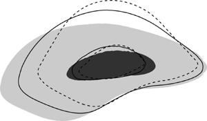
Before presenting the result of the optimisation formulated in § 2, it is useful to discuss some key features of the spectra from a high-Reynolds-number DNS (Lee & Moser Reference Lee and Moser2015), ${\boldsymbol \varPhi _{\boldsymbol uu}^{DNS}}(k_x,k_z,y)$. Figure 1 shows the normalised two-dimensional spectra for $k_zh = 14, 30, 50$ plotted in self-similar coordinates $(y/\lambda _z, \lambda _x/\lambda _z)$, where $\lambda _x=2{\rm \pi} /k_x$ and $\lambda _z=2{\rm \pi} /k_z$. The self-similarity in the spectra is clearest in the wall-normal velocity spectra and Reynolds shear stress co-spectra (figure 1b,d), with the latter defining the ‘active’ contributions of the energy-containing eddies (Townsend Reference Townsend1976; Hwang Reference Hwang2015; Deshpande et al. Reference Deshpande, Monty and Marusic2021). Both the streamwise and spanwise velocity spectra exhibit self-similarity for the high-level contours: the streamwise velocity spectra have the peak at $\lambda _x \approx 10 \lambda _z$ and $y \approx 0.1 \lambda _z$, representing streaks, while the spanwise velocity spectra show the energetic peak at $\lambda _x \approx 1-2 \lambda _z$ and $y \approx 0.1-0.2 \lambda _z$ representing the vortex packets involving streak instability (Hwang Reference Hwang2015; de Giovanetti et al. Reference de Giovanetti, Sung and Hwang2017). Consistent with Townsend's attached eddy hypothesis, the wall-reaching footprints of the energy-containing attached eddies are seen in the wall-parallel velocity spectra, especially for large $\lambda _x$ (see $y/\lambda _z\lesssim 0.05$ in figure 1a,c). These footprints are inactive in a sense that there is no contribution to the Reynolds shear stress (figure 1d) and they break the self-similarity in the near-wall vicinity (Hwang Reference Hwang2015Reference Hwang2016). In the self-similar coordinates, the relative contribution of this inactive footprint to the wall-parallel velocity spectra grows with the spanwise wavelength such that the eddies remain attached.

Figure 1. Premultiplied two-dimensional spectra for $k_zh = 14$ (shaded), 30 (solid), 50 (dashed) ($\lambda _z/h\approx 0.45, 0.21, 0.13$; $\lambda _z^+\approx 2300, 1100, 650$) of (a) streamwise, (b) wall-normal and (c) spanwise velocities and (d) Reynolds shear stress. Here the spectra are normalised and the selected contour levels are $0.20$ and $0.80$ of the maximum. The horizontal and vertical pairs of dashed lines in (ac) are for $y/\lambda _z = 0.1$, $\lambda _x/\lambda _z = 10$ and $y/\lambda _z = 0.5$, $\lambda _x/\lambda _z = 2$ respectively.

A second self-similar breaking feature is present in all the spectra for small streamwise wavelengths ($\lambda _x/\lambda _z\lesssim 1$) and is also prominent in the region relatively far away from the wall ($y/\lambda _z\gtrsim 0.5$). This region depicts small-scale detached eddies associated with energy cascade, transporting turbulent kinetic energy from the integral length scale down towards smaller length scales to be dissipated. In wall-bounded turbulence, the presence of the wall imposes the integral length scale to follow distance from the wall, with the relevant integral length scale following $\delta _\nu$ ($\equiv \nu /u_\tau$), $y$ and $h$ at the inner, logarithmic and outer regions respectively. The Kolmogorov length scale at which dissipation occurs is given by $\delta _\nu$, $(y\delta _\nu ^3)^{1/4}$ and $(h\delta _\nu ^3)^{1/4}$ in the inner, logarithmic and outer regions respectively. This leads to a large separation between the integral and dissipation length scales, following $Re_\tau ^{3/4}(y/h)^{3/4}$ in the logarithmic region (Lee & Moser Reference Lee and Moser2019). The streamwise wavelengths (or wavenumbers) between the two length scales are in the inertial subrange (Pope Reference Pope2000), and this is present approximately in the region of $\lambda _x/\lambda _z \lesssim 1$ (i.e. streamwise length scales smaller than the peak location in the spectra). As $k_z$ is decreased (or $\lambda _z$ is increased), the intensity of the spectra in the inertial subrange is expected to gradually increase, due to the increase in integral length scale $y$ from the self-similar peak scaling and large separation to the dissipation length scale. This is observed for $\lambda _x/\lambda _z\lesssim 1$ in figure 1. In particular, given that the small-scale motions related to the energy cascade are expected to be highly isotropic (Kolmogorov Reference Kolmogorov1991), this feature is more obvious in the velocity spectra (figure 1ac), which exhibit increasing energy for $\lambda _x/\lambda _z\lesssim 1$ with decreasing $k_z$ (or increasing $\lambda _z$). However, it is much less noticeable in the Reynolds shear stress co-spectra due to the increased isotropy at small length scales: the Reynolds shear stress co-spectra are expected to exhibit a relatively rapid decay following a $-7/3$ power law in comparison with the $-5/3$ power law for the velocity spectra (Lumley Reference Lumley1967). For a detailed discussion on the spectra of the energy cascade, the reader may also refer to Cho et al. (Reference Cho, Hwang and Choi2018), Lee & Moser (Reference Lee and Moser2019) and Hwang & Lee (Reference Hwang and Lee2020).

4. Results

4.1. Optimal forcing at a single spanwise length scale

The performance of the linearised model is first evaluated with the optimal white-noise forcing at spanwise wavenumber $k_zh=14$, primarily related to the logarithmic region (i.e. $\lambda _z \approx 0.45h$ or $\lambda _z^+ \approx 2333$). A similar qualitative trend is found across the spanwise wavenumbers, with difference across the spanwise wavenumbers discussed in § 4.3. A comparison of the premultiplied two-dimensional spectra between the DNS (solid contours) and linear model (shaded contours) is shown in figure 2. All of the qualitative features are reproduced by the linear model with relative errors $\epsilon _s$, defined as

(4.1)\begin{equation} \epsilon_s = \frac{\left|\left| \boldsymbol \varPhi^{DNS}_{s} - \boldsymbol \varPhi_{s}(W_r)\right|\right|_Q}{\left|\left| \boldsymbol \varPhi^{DNS}_{s}\right|\right|_Q}, \end{equation}

for $s = \{uu, vv, ww, uv\}$ being (0.20, 0.087, 0.081, 0.55) respectively. Note that these quantitative errors reflect the difference between the linear model's spectra and the relatively noisy two-dimensional DNS spectra. Therefore, an unknown level of the error can be attributed to denoising the DNS spectra, smoothing out the numerical/statistical noise from a finite sampling time interval.

Figure 2. Premultiplied two-dimensional spectra in self-similar coordinates for $k_z = 14/h$, $k_z^+ = 0.0027$ ($\lambda _z = 0.45h$, $\lambda _z^+ = 2333$) of (a) streamwise, (b) wall-normal and (c) spanwise velocities and (d) Reynolds stress. Here the shaded contours indicate DNS spectra and the solid contours are optimisation results from (2.19). The contour levels are separated by 0.20 times the maximum value for each spectrum.

The streamwise velocity spectra from the linear model (figure 2a) have a good qualitative agreement with those of DNS. The location of the primary peak associated with the energy-containing eddies approximately replicated aligns with the DNS peak. The linear model also well replicates the low-level contour region in the DNS spectra associated with the energy cascade ($\lambda _x/\lambda _z \lesssim 0.5$ and $y/\lambda _z \gtrsim 0.05$). In particular, the wall-normal and spanwise velocity spectra (figure 2b,c) show an almost exact qualitative and quantitative match, with a majority of the error presumably from the denoising of the DNS result. However, it is clear by comparison of the figures and in the relative error that the linear model performs relatively poorly in generating the correct Reynolds shear stress co-spectra. A significant region in the spectra away from the wall is not reproduced by the linear model. To further examine the relative error between the normalised spectra defined as

(4.2)\begin{equation} \tilde{\epsilon}_s = \left|\left| \frac{\varPhi_s}{\left|\left| \varPhi_{s}\right|\right|_Q} - \frac{\varPhi_s^{DNS}}{\left|\left| \varPhi_{s}^{DNS}\right|\right|_Q}\right|\right|_Q, \end{equation}

the ratio of the two norms

(4.3)\begin{equation} \rho_s = \frac{\left|\left| \varPhi_{s}\right|\right|_Q}{\left|\left| \varPhi_{s}^{DNS}\right|\right|_Q} \end{equation}

is evaluated for $s = \{uu, vv, ww, uv\}$. Here (4.3) is the ratio of the logarithmic weighted Reynolds stresses at the given $k_zh$. For the Reynolds shear stress co-spectra, $\tilde {\epsilon }_{uv} = 0.29$ and $\rho _{uv} = 0.49$. This indicates that the linear model can reproduce the structure of the Reynolds shear stress co-spectra reasonably well (compare this with $\epsilon _{uv} = 0.55$), but the difference in norms of the spectra suggests the linear model generates a relatively weak Reynolds shear stress. This is similarly argued by the ratio of the two peaks in the Reynolds shear stress spectra being 0.44. The reason for this large discrepancy in the amplitude is likely due to the functional approximation of the forcing, with the optimisation problem restricting the forcing input to be white-in-time and spatially decorrelated. The lack of significant cross-correlation between the streamwise and wall-normal forcing components, which would be present in the exact nonlinear term (Jovanovic & Bamieh Reference Jovanovic and Bamieh2001; Chevalier et al. Reference Chevalier, Hœpffner, Bewley and Henningson2006; Morra et al. Reference Morra, Nogueira, Cavalieri and Henningson2021), leads to these relatively low Reynolds shear stresses. It is likely that a more carefully chosen eddy viscosity term can improve this feature, i.e. further modification of the linear dynamical operator (for an early discussion, see also Jovanovic & Bamieh (Reference Jovanovic and Bamieh2001)) or, alternatively, relaxing the white-in-time assumption. This issue can be resolved by a data-driven approach such as that in Zare et al. (Reference Zare, Jovanović and Georgiou2017); however, such an approach required the $\boldsymbol B$ operator to be modified. This would change the way in which the nonlinear term drives the linearised dynamics, limiting the physical interpretability of the forcing. As discussed in § 2, the eddy viscosity here provides an explicit simple approach in modifying the nonlinear term across wavenumbers, helping to at least partially replicate the nonlinear term (Hwang Reference Hwang2016; Hwang & Eckhardt Reference Hwang and Eckhardt2020; Pickering et al. Reference Pickering, Rigas, Schmidt, Sipp and Colonius2021; Symon et al. Reference Symon, Illingworth and Marusic2021).

The forcing spectra which drive the corresponding response in figure 2 are shown in figure 3. All of the forcing spectra exhibit a smoothly varying structure with a primary peak which drives the energy-containing motions in the corresponding velocity spectra. It is interesting to note that the primary peak locations of all the spectra are around $\lambda _x/\lambda _z \approx 1$ and $y/\lambda _z \approx 0.2\unicode{x2013}0.7$. This behaviour is different from that in the velocity spectra. In particular, the streamwise velocity spectra contain the primary peak at a much longer streamwise wavelength in the region relatively close to the wall: $\lambda _x/\lambda _z \approx 10$ and $y/\lambda _z \approx 0.1$ (figure 2a). Outside of this primary peak location, in general, the forcing spectra tend to be much more intense at shorter streamwise wavelengths than the velocity spectra (compare figure 3 with figure 2). The velocity spectra contain very little energy for $\lambda _x/\lambda _z\lesssim 0.1$ (figure 3), while all the forcing spectra contain a considerable amount of energy (figure 2). This is because of the effect of the viscous diffusion operator in the linear model becoming increasingly stronger as $\lambda _x$ decreases. Overall, this results in a relatively energetic forcing input required to generate even a weak velocity spectrum. Similarly, the eddy viscosity in (2.2b) considered for the linear model grows linearly with the distance from the wall in the logarithmic region due to

(4.4)\begin{equation} -\frac{\overline{u'v'}}{u_\tau^2}=\nu_t \frac{{\rm d} U}{{\rm d}y}, \end{equation}

where $\overline {u'v'}$ is approximately constant (Townsend Reference Townsend1976; Pope Reference Pope2000), leading to $\nu _t \sim y$ from the logarithmic mean velocity. Therefore, the forcing spectra tend to be relatively more energetic than the velocity spectra away from the wall ($y/\lambda _z \gtrsim 0.5$). All these observations suggest that a significant portion of the energetic part of the forcing spectra plays a role of driving the velocity spectra associated with energy cascade and dissipation in DNS. These features are noticeable in all of the forcing components, the spectra of which contain more than half of the total energy for $\lambda _x/\lambda _z \lesssim 1$ or $y/\lambda _z \gtrsim 1$ (figure 3). This is in contrast to the velocity spectra in figure 2. The streamwise velocity spectra (figure 2a) and the Reynolds shear stress co-spectra (figure 2d) are seen to carry little energy for $\lambda _x/\lambda _z \lesssim 1$ or $y/\lambda _z \gtrsim 1$. The exact contribution of these forcing spectra to the velocity spectra response is discussed in componentwise terms in the following section (see also § 5.2).

Figure 3. Premultiplied two-dimensional spectra in self-similar coordinates for $k_zh = 14$, $k_z^+ = 0.0027$ ($\lambda _z = 0.45h$, $\lambda _z^+ = 2333$) of (a) streamwise, (b) wall-normal and (c) spanwise forcing components and (d) the total forcing spectra. The contour levels are separated by 0.1 times the maximum value for each spectrum. The horizontal dashed lines show $y/\lambda _z = 0.5$ and the vertical dashed lines show $\lambda _x/\lambda _z = 1$.

With the forcing spectra as shown in figure 3 and as described previously, caution is needed to understand what the forcing term would represent. In particular, for the model of the nonlinear term $\mathcal {N}$, an eddy viscosity diffusion term was included, i.e. $\mathcal {N}_{\nu _t,f}$ in (2.2a). Therefore, the forcing spectra are not directly comparable with the spectra of the nonlinear term $\mathcal {N}$. The eddy viscosity term modifies the linear dynamical operator, providing a mechanism to dissipate the energy at large scale by replacing a role of the nonlinear term $\mathcal {N}$ that transfers the energy from large to small scale (see Symon et al. (Reference Symon, Madhusudanan, Illingworth and Marusic2022) for a more detailed discussion). Furthermore, the forcing is also crudely assumed spatially decorrelated and white-in-time. Hence, the forcing spectra shown here would only phenomenologically mimic some partial roles of the nonlinearity. That being said, it is finally worth mentioning the recent work by Morra et al. (Reference Morra, Nogueira, Cavalieri and Henningson2021), who showed that a combination of the current eddy viscosity model with rank-1 approximation using the leading resolvent modes provides a fairly good proxy for the nonlinear term, at least for a certain set of spatial wavenumbers and frequencies that admit strong linear amplification. In this respect, the current model is expected to perform well, at least for such a set of spatial wavenumbers and frequencies, as the stochastic response would be dominated by the leading resolvent modes.

4.2. Componentwise breakdown of the stochastic forcing

To further assess the role of the forcing structure, the linear nature of the model can be exploited as in § 2.3, with the total response being the superposition of the spectra driven by each of the forcing components individually. It should be stressed that setting all but one of the forcing components to zero is non-physical (see § 5 for further details), as the covariance of the forcing which generates the velocity spectra has to be solenoidal (see § 5 for further details and Rosenberg & McKeon (Reference Rosenberg and McKeon2019) and Morra et al. (Reference Morra, Nogueira, Cavalieri and Henningson2021)). However, the subsequent analysis still holds significance for modelling strategies that may independently modify each of the forcing components. Indeed, it allows us to understand which part of the spectra is effectively modelled by the different forcing components under the linear amplification mechanisms and which part is only modelled phenomenologically with the nonlinear term model in (2.2a).

Figures 4(a), 4(d), 4(g) and 4(j) show the streamwise, wall-normal and spanwise velocity spectra and Reynolds shear stress co-spectra respectively with only the streamwise component of the forcing spectra active (figure 3a) and the remaining components set zero. The spectra are normalised by the maximum values of the spectra with all forcing components, indicating the relative contribution of each of the forcing components to the response shown in figure 2. Figure 4(a) shows the forcing in the streamwise component has a significant (${\approx }70\,\%$ of the total response maximum) contribution in driving the streamwise velocity spectra, with the peak located at $\lambda _x/\lambda _z \approx 3$ and $y/\lambda _z \approx 0.3$. Figure 4(a) also demonstrates that the forcing in the streamwise velocity component yields little to no contribution to the near-wall inactive part of the streamwise velocity spectra, except the short streamwise wavelength around $\lambda _x/\lambda _z \approx 2$, when compared with the total response (compare figure 4a with figure 2a). Aside from the driving of the primary peak, it is seen that the streamwise forcing component drives a response in the streamwise velocity associated with energy-cascade-related region of the DNS spectra ($\lambda _x/\lambda _z \lesssim 1$ in figure 4a), although this is not clear due to the presence of the strong primary peak (see also discussion below). The relative contribution of the streamwise forcing component to the other spectra is less significant than that to the streamwise velocity itself, providing a small contribution in close proximity to the primary peak of the other spectra (figure 4d,g,j). Additionally, the forcing in the streamwise velocity component drives relatively more significant contributions to those at small streamwise wavelengths associated with energy cascade in the wall-normal velocity spectra and Reynolds shear stress co-spectra ($\lambda _x/\lambda _z\lesssim 1$ and $y/\lambda _z \gtrsim 0.05$ in figure 4d,j). In particular, comparing figure 4(j) with figure 4(k,l) shows that the streamwise forcing component exclusively drives the small-scale response in the Reynolds shear stress co-spectra.

Figure 4. Premultiplied two-dimensional spectra in self-similar coordinates for $k_z = 14/h$, $k_z^+ = 0.0027$ ($\lambda _z = 0.45h$, $\lambda _z^+ = 2333$) of (ac) streamwise, (df) wall-normal and (gi) spanwise velocities and (jl) Reynolds stress with the forcing intensity (a,d,g,j) $\boldsymbol \varOmega _u$, (b,e,h,k) $\boldsymbol \varOmega _v$ and (c,f,i,l) $\boldsymbol \varOmega _w$. Here the contour levels are separated by 0.10 times the maximum value of the spectra with total forcing intensity $\boldsymbol \varOmega$.

Figures 4(b) 4(e), 4(h) and 4(k) show the streamwise, wall-normal and spanwise velocity spectra and Reynolds shear stress co-spectra respectively with only the wall-normal component (figure 3b) of the forcing active. Here the response is most strongly coupled, with the wall-normal forcing providing significant relative contributions in the streamwise and wall-normal velocity spectra and Reynolds shear stress co-spectra (figure 4b,e,k). The response in the streamwise velocity spectra shows how the forcing in the wall-normal component is responsible for driving a portion of the response close to the primary peak of the total streamwise velocity spectra (figure 4b). Importantly, it drives the near-wall inactive footprint, with this response being almost exclusive to the wall-normal forcing for large streamwise wavelengths (compare figure 4b with figure 4a,c). The effect of the wall-normal forcing component on the wall-normal velocity spectra is similar to that of the streamwise forcing component on the streamwise velocity, with the forcing driving a majority of the primary peak, as well as the small-scale features that statistically mimic the energy cascade region from DNS (figure 4e). The wall-normal forcing is responsible for driving a majority ($\approx$70 % of the maximum total response) of the primary peak in the Reynolds shear stress co-spectra and almost the entire response in the Reynolds shear stress for large streamwise wavelengths (figure 4jl).

Lastly, figures 4(c), 4(f), 4(i) and 4(l) show the streamwise, wall-normal and spanwise velocity spectra and Reynolds shear stress co-spectra respectively with only the spanwise component (figure 3c) of the forcing active. As before, the spanwise forcing component drives a majority of the primary peak in the spanwise velocity spectra, as well as the small-scale features associated with the energy cascade. In contrast to the inactive near-wall footprint of the streamwise velocity spectra, which is not mainly generated by the streamwise forcing component (see figure 4ac), the inactive footprint of the spanwise velocity spectra is primarily generated by the corresponding spanwise forcing, with some contribution from the streamwise and wall-normal forcing components (see $y/\lambda _z\lesssim 0.05$ in figure 4gi). The spanwise forcing component also tends to drive a portion of the the near-wall inactive features in the streamwise velocity spectra (figure 4c), although much less significant than the wall-normal forcing (compare with figure 4b). The effect of the spanwise forcing component on the wall-normal velocity spectra and Reynolds shear stress co-spectra is similar to that of the streamwise forcing component. The contribution of the spanwise forcing appears closer to the primary peaks, however (compare figures 4f,l and 4d,j). Moreover, the effect of the spanwise forcing component appears to be shifted more towards larger streamwise wavelengths (see also § 5.2).

Overall, figure 4 reveals how the given two-dimensional velocity spectra in the $\lambda _x$$y$ plane for a spanwise length scale $\lambda _z$ (or wavenumber $k_z$) can be modelled componentwise through a white-in-time and spatially decorrelated stochastic forcing, augmented with an eddy viscosity diffusion operator in (2.2b). Given the linearised nature of (2.1a) about a parallel base flow, with the (linear) model term $\mathcal {N}_{\nu _t,f}$, the Reynolds shear stress generation (or production) of the model is only facilitated through the lift-up effect (e.g. Butler & Farrell Reference Butler and Farrell1993; del Álamo & Jiménez Reference del Álamo and Jiménez2006; Hwang & Cossu Reference Hwang and Cossu2010a; McKeon & Sharma Reference McKeon and Sharma2010) and the Orr mechanism (Jiménez Reference Jiménez2013; Encinar & Jiménez Reference Encinar and Jiménez2020; Doohan, Willis & Hwang Reference Doohan, Willis and Hwang2021; Jiao, Hwang & Chernyshenko Reference Jiao, Hwang and Chernyshenko2021). The former is clearly well captured by the model from figure 4(b,k), showing a strong response of streamwise velocity to the given wall-normal forcing at long streamwise length scales ($\lambda _x/\lambda _z\approx 10$). The latter is seen in figure 4(e), depicting the amplification of wall-normal velocity in response to a wall-normal forcing at relatively short length scales ($\lambda _x/\lambda _z\approx 1\unicode{x2013}2$). Figure 4(jl) indicates that the Reynolds shear stress co-spectra are dominantly produced by the wall-normal forcing component through these mechanisms. This is presumably a consequence of the linear model directly facilitating the two mean-shear-driven processes responsible for turbulence production (i.e. the lift-up effect and the Orr mechanism). Further details of this issue are discussed in § 5.2.

It is also important to mention that a considerably large amount of streamwise and spanwise forcing is needed to fully capture the energetic part of the streamwise and spanwise velocity spectra seen in figure 4(a,i). The peak locations in figure 4(a,i) are at $\lambda _x/\lambda _z \approx 1\unicode{x2013}3$ and $y/\lambda _z\approx 0.3$, aligning well with $\lambda _x/\lambda _z \approx 3$ and $y/\lambda _z\approx 0.3$ predicted by the streak instability (Alizard Reference Alizard2015; de Giovanetti et al. Reference de Giovanetti, Sung and Hwang2017). This suggests that the forcing of the linear model, with the mean velocity dependent only on wall-normal location, is entirely phenomenological for this response. In real flow, there are other important physical processes of generating spectral energy without directly involving the mean shear. Finally, it should be emphasised that the energy cascade and the wall-reaching inactive part of the spectra are also captured only phenomenologically, considering they originate from the intrinsic nonlinear processes of $\mathcal {N}$. The forcing required to mimic the velocity spectra associated with energy cascade is relatively strong, as shown in figure 3 and discussed in § 4.1. However, it is worth noting that the velocity spectra associated with the energy cascade and the wall-reaching inactive part are much weaker than those of the energy-containing counterpart. In other words, a precise description of the forcing structure for the energy cascade and the wall-reaching inactive part may not be necessary for modelling of the energy-containing region in the velocity spectra.

In summary, the forcing spectra are composed of parts of modelling energetic (i.e. energy-containing region) and non-energetic (i.e. energy cascade region featured by a decay of energy with a $k^{-5/3}$ law) regions of velocity spectra (see also discussion in § 3). The former part of the forcing spectra would not need large energy. As is well known (Jovanovic & Bamieh Reference Jovanovic and Bamieh2005), the linear amplification mechanisms (i.e the lift-up and the Orr mechanisms) are expected to play a role in effectively generating the energetic part of velocity spectra. However, it is unclear if the latter is also the case, given the non-energetic nature of the velocity spectra. Furthermore, it is unclear if the lift-up or the Orr mechanism would also play any role in modelling the non-energetic part of velocity spectra. The componentwise analysis showed that each component of the non-energetic region of velocity spectra is mainly modelled by the corresponding component of the forcing with relatively large energy input, suggesting that the lift-up and the Orr mechanisms are not highly active in modelling the non-energetic part of the spectra. This also implies that forcing at each component can suitably be tailored to model the non-energetic region of the corresponding component of the velocity spectra.

4.3. Self-similarity and non-self-similarity of forcing spectra across scales

The stochastic forcing is now determined for spanwise wavelengths ranging from outer to inner length scales, i.e. $\lambda _z/h \approx 1$ to $\lambda _z^+ \approx 100$, with results shown in table 1. Figure 5 shows the velocity spectra and Reynolds shear stress co-spectra for an outer length scale of $\lambda _z/h \approx 1$ ($k_zh = 6$) associated with large-scale and very-large-scale motions (figure 5a,d,g,j), an inner length scale of $\lambda _z^+ \approx 100$ ($k_zh= 326$) associated with the spacing of near-wall streaks and quasi-streamwise vortices (figure 5c,f,i,l) and an intermediate logarithmic region length scale of $\lambda _z/h \approx 0.2$ ($k_zh = 30$) (figure 5b,e,h,k). The streamwise velocity spectra modelled (figure 5ac) exhibit a similar match to those from DNS, with a strong agreement across all spanwise wavelengths considered. The primary peak occurs at approximately the same streamwise wavelength, with this peak shifted closer to the wall in comparison with the DNS due to the driving of the wall-reaching part of the spectra through the wall-normal forcing component (figure 4b). This distortion to the velocity spectra peak becomes less noticeable for smaller spanwise wavelengths (figure 5c, in particular). In fact, for the smallest spanwise wavelength considered ($\lambda _z^+ \approx 100$), there are no inactive features in the spectra since the active part occurs adjacent to the wall. However, at this spanwise length scale, the linear model produces a much more localised response about the primary peak (figure 5c). The velocity spectra produced with the optimal white-noise forcing decay much more rapidly than the DNS spectra, especially above the primary peak. This results in comparatively large errors in the near-wall region (compare $\epsilon _{uu}$ for $k_zh = 326$ with $k_zh = 14, 30 ,50$ in table 1). Likewise to the results at $k_zh = 14$ (figure 2), the strongest match is that of the wall-normal velocity spectra for all spanwise wavelengths considered (figure 5df). The spanwise velocity spectra exhibit a similar trend to the streamwise velocity spectra, although the location of the primary peak is more consistent with the DNS velocity spectra when compared with the streamwise velocity spectra (compare figure 5ac with figure 5gi). Much like the streamwise velocity case for the smallest considered spanwise wavelength, the spanwise velocity spectra have a significantly reduced response for the part above the primary peak (figure 5i). Lastly, like the $k_zh = 14$ case (figure 3), the Reynolds shear stress co-spectra (figure 5jl) always have the largest relative error. This error is due to a low amplitude of Reynolds shear stress generated and poor replication of the spectra above the primary peak, as indicated by the ratio of the norms and relative error between the normalised spectra.

Figure 5. Premultiplied two-dimensional spectra in self-similar coordinates: (a,d,g,j) $k_zh = 6$ ($\lambda _z/h \approx 1.05$); (b,e,h,k) $k_z h= 30$ ($\lambda _z/h \approx 0.21$ or $\lambda _z^+ \approx 1100$); (c,f,i,l) $k_z^+ \approx 0.0064$ ($\lambda _z^+ \approx 100$). (ac) Streamwise velocity spectra, (df) wall-normal velocity spectra, (gi) spanwise velocity spectra and (jl) Reynolds shear stress co-spectra. The shaded contours indicate DNS spectra and the solid contours are optimisation results from (2.19).The contour levels are separated by 0.20 times the maximum value of the spectra with forcing intensity $\boldsymbol \varOmega$ for comparison.

Table 1. The optimisation errors defined in (4.1)–(4.3) for the different spanwise wavelengths. Regularisation weighting $\gamma$ and number of sine polynomials used $N_s$ are reported together.

The self-similarity of the forcing spectra is examined in figure 6. The spatially decorrelated forcing spectra are considered for spanwise wavenumbers, $k_zh = 14,30,50$, primarily associated with the logarithmic region. Here, the contour levels were chosen to be $0.8$ and $0.2$ times the maximum values to highlight the regions of the forcing associated with the self-similar energy-containing motions and the self-similar breaking regions respectively. Both of the wall-parallel velocity spectra show approximate self-similar peaks at $y/\lambda _z \approx 0.3\unicode{x2013}1$ and $\lambda _x/\lambda _z \approx 1$. Given that the primary peaks are associated with the energy-containing features in the velocity spectra, this is consistent with the attached eddy hypothesis (Townsend Reference Townsend1976), and self-similarity present in the DNS spectra and linearised Navier–Stokes equations, although there is some disparity in the wall-normal forcing spectra with the high-level contours growing with spanwise length scale.

Figure 6. Premultiplied two-dimensional spectra in self-similar coordinates for the (a) streamwise, (b) wall-normal and (c) spanwise forcing components and (d) total forcing. Here the spanwise length scales are $k_zh = 14$ (shaded), $30$ (solid), $50$ (dashed). The contour levels are chosen to be $0.2$ and $0.8$ times the maximum value.

It is, however, worth noting that the overall level of self-similarity in the forcing spectra is not as convincing as that in the velocity spectra (see also figure 1). In particular, in the regions of the forcing spectra that drive a response in the velocity spectra associated with the energy cascade ($\lambda _x/\lambda _z \lesssim 1$ or $y/\lambda _z \gtrsim 1$), the intensity grows with $\lambda _z$. Note that the non-self-similar part of the forcing spectra does not make a strong contribution to the velocity spectra. If it did, the resulting velocity spectra should also have this same level of non-self-similar behaviour as well, but this was not the case (figures 1 and 5). As discussed in § 4.1, the linear model is strongly influenced by the diffusion operator in these regions due to the short streamwise wavelengths and the eddy viscosity growing only with $y$. Therefore, the forcing spectra in this region are relatively energetic when compared with the velocity spectra, revealing more clearly the non-self-similar nature originating from the velocity spectra. This is most clear in the wall-normal forcing spectra, where there is substantial forcing input at these short streamwise wavelengths, breaking self-similarity. On the contrary, the non-self-similarity in the forcing spectra associated with the wall-reaching near-wall part in the velocity spectra ($y/\lambda _z \lesssim 0.05$ for $\lambda _x/\lambda _z \gtrsim 1$) is not very prominent in figure 6. This indicates that the main driver of the non-self-similarity associated with the wall-reaching near-wall part in the velocity spectra is likely to be the eddy viscosity varying with $y$, driving near-wall features through the lift-up effect (see also §§ 5.2 and 5.3). This is consistent with the previous observation by Hwang (Reference Hwang2016), who argued that the wall-reaching near-wall part of the response from the linear model originates from the eddy viscosity.

In short, although the velocity spectra are seen to be largely self-similar due to their energy-containing part consistent with the attached eddy hypothesis, they are precisely not self-similar due to the parts related to energy cascade and inactive motions (see § 3). These non-self-similar parts are strongly amplified in the forcing spectra, because the given linear operator does not contain an efficient transfer mechanism (e.g. lift-up and Orr mechanisms) of the forcing to the velocity at the related spatial wavelengths (e.g. $\lambda _x/\lambda _z \lesssim 1$; see also Hwang & Cossu Reference Hwang and Cossu2010a).

5. Discussion

5.1. Solenoidal forcing structure

To more precisely assess the role of the forcing and its contribution in driving the velocity spectra, attention is now turned to the solenoidal component of the forcing. Specifically, the forcing can be projected onto a solenoidal field and an irrotational field:

(5.1)\begin{equation} \hat{\boldsymbol f} = \hat{\boldsymbol f}^s + \hat{\boldsymbol f}^r, \end{equation}

where $\boldsymbol {\nabla }\boldsymbol {\cdot } \hat {\boldsymbol f}^s = 0$ and $\boldsymbol {\nabla } \times \hat {\boldsymbol f}^r = 0$. This is done as only the solenoidal component of the forcing contributes to the driving of velocity fluctuations, since the irrotational component is in the null space of the $\boldsymbol B$ operator (Rosenberg & McKeon Reference Rosenberg and McKeon2019; Morra et al. Reference Morra, Nogueira, Cavalieri and Henningson2021). With regard to the optimisation forcing input, it can be shown that this spatially decorrelated forcing cannot be solenoidal. By considering

(5.2)\begin{equation} \widehat{\boldsymbol{\nabla}\boldsymbol{\cdot} \boldsymbol f} = \boldsymbol E \hat{\boldsymbol f}, \quad \text{where}\ \boldsymbol E = [{\rm i}k_x \quad \mathcal{D} \quad {\rm i}k_z], \end{equation}

which gives the covariance operator for the forcing divergence as

(5.3)\begin{equation} R_{\widehat{\boldsymbol{\nabla}\boldsymbol{\cdot} \boldsymbol f} \widehat{\boldsymbol{\nabla}\boldsymbol{\cdot} \boldsymbol f}} = \boldsymbol E \boldsymbol R_{\hat{\boldsymbol f}\hat{\boldsymbol f}}\boldsymbol E^{{{\dagger}}}. \end{equation}

In the case of the spatially decorrelated forcing input, this gives

(5.4)\begin{equation} R_{\widehat{\boldsymbol{\nabla}\boldsymbol{\cdot} \boldsymbol f} \widehat{\boldsymbol{\nabla}\boldsymbol{\cdot}\boldsymbol f}} = k_x^2R_{\hat{f}_u\hat{f}_u}(y) + R_{\mathcal{D}\hat{f}_v\mathcal{D} \hat{f}_v}(y) + k_z^2 R_{\hat{f}_w\hat{f}_w}(y), \end{equation}

and therefore $\mathbb {E}[|\widehat {\boldsymbol {\nabla }\boldsymbol {\cdot } \boldsymbol f}|^2] > 0$ for any $\boldsymbol f \ne \boldsymbol 0$. Consequently the forcing input from the optimisation is not solenoidal, and must be further manipulated to determine the solenoidal forcing which drives the linear dynamics. This is also expected in the case of typical frequency-domain analysis, where the autocorrelation of the forcing at a given frequency is often assumed to be spatially decorrelated (see e.g. Towne, Schmidt & Colonius Reference Towne, Schmidt and Colonius2018). This assumption would lead to a ratio of solenoidal and irrotational forcing to affect the velocity and pressure field respectively, dependent on the wavenumbers (see also discussion below).

To recover the solenoidal forcing component, Morra et al. (Reference Morra, Nogueira, Cavalieri and Henningson2021) is followed with $\boldsymbol B \hat {\boldsymbol f} = \boldsymbol B {\hat {{\boldsymbol f}}}^s = \boldsymbol D \boldsymbol {\hat {{\boldsymbol f}}}^s$ and since $\hat {\boldsymbol u} = \boldsymbol C \hat {\boldsymbol q} = \boldsymbol C \boldsymbol D \hat {\boldsymbol u}$, where

(5.5)\begin{equation} \boldsymbol D = \begin{bmatrix}0 & 1 & 0\\ {\rm i}k_z & 0 & -{\rm i}k_x \end{bmatrix}, \end{equation}

the covariance operator of the solenoidal forcing component is determined through

(5.6)\begin{equation} \boldsymbol R_{\widehat{\boldsymbol f^{s}}\widehat{\boldsymbol f^{s}}} = \boldsymbol C \boldsymbol B \boldsymbol R_{\hat{\boldsymbol f}\hat{\boldsymbol f}} \boldsymbol B^{{{\dagger}}} \boldsymbol C^{{{\dagger}}}. \end{equation}

Similarly, since $\hat {\boldsymbol f}^r = (\boldsymbol I - \boldsymbol C \boldsymbol B)\hat {\boldsymbol f}$, the covariance operator of the irrotational forcing component is given by

(5.7)\begin{equation} R_{\widehat{\boldsymbol f^{r}}\widehat{\boldsymbol f^{r}}} = (\boldsymbol I - \boldsymbol C \boldsymbol B) R_{\hat{\boldsymbol f}\hat{\boldsymbol f}} (\boldsymbol I - \boldsymbol C \boldsymbol B)^{\dagger}. \end{equation}

Figures 7(a)–7(c) show the spectra of the solenoidal streamwise, wall-normal and spanwise forcing respectively. By comparing these with figure 3(ac), there is a great deal of similarity in the streamwise and spanwise forcing spectra (figure 3a,c), with the same qualitative features present and the magnitude of the spectra being approximately the same. However, there is a stark contrast between the wall-normal forcing spectra and the solenoidal counterpart (figures 3b and 7c). In particular, the solenoidal wall-normal forcing is seen to spend relatively larger amounts of energy in mimicking energy cascade features, considering the energetic region of its spectra corresponds to the region of energy cascade in the velocity spectra ($\lambda _x/\lambda _z \lesssim 10^{-1}$, $y/\lambda _z \lesssim 0.5$). Given that the velocity spectra related to energy cascade are not self-similar with $y$ (or $\lambda _z$), and the scale-dependent effect of the viscous diffusion operator in the linear model (see the discussion in § 4.1), it can be expected that the solenoidal wall-normal forcing spectra should behave similarly to the energy cascade scaling features in the wall-normal velocity spectra (see also figure 8a).

Figure 7. Premultiplied two-dimensional spectra in self-similar coordinates for $k_zh = 14$, $k_z^+ = 0.0027$ ($\lambda _z = 0.45h$, $\lambda _z^+ = 2333$) of (a) streamwise, (b) spanwise, (c) wall-normal and (d) energy inner-product weighted wall-normal solenoidal forcing spectra. The contour levels are separated by 0.1 times the maximum value for each spectrum. The horizontal dashed lines show $y/\lambda _z = 0.5$ and the vertical dashed lines show $\lambda _x/\lambda _z = 1$.

Figure 8. Premultiplied two-dimensional solenoidal forcing spectra in self-similar coordinates for (a) the wall-normal component and (b) the wall-normal component with respect to the energetic inner product. The spanwise length scales are $k_zh = 14$ (shaded), $30$ (solid), $50$ (dashed). The contour levels are chosen to be $0.2$ and $0.8$ times the maximum value.

To understand how the solenoidal part of the wall-normal forcing loses the strong self-similarity observed in the original wall-normal forcing spectra, or equivalently how the modelling of energy cascade features masks any self-similar behaviour, the Orr–Sommerfeld–Squire system can be reconsidered. Since only the solenoidal component can alter the $\hat {\boldsymbol q}$ state, assume $\hat {\boldsymbol f} = \widehat {\boldsymbol f^s}$, with the statistics of the solenoidal forcing of the optimised forcing input readily determined from (5.6). This gives the following evolutionary equation for $\hat {\boldsymbol q}$:

(5.8)\begin{equation} \frac{\partial \hat{\boldsymbol q}}{\partial t} = \boldsymbol A \hat{\boldsymbol q} + \boldsymbol D \hat{\boldsymbol f}^s, \end{equation}

with corresponding Lyapunov equation

(5.9a)\begin{equation} \boldsymbol A \boldsymbol R_{\hat{\boldsymbol q}\hat{\boldsymbol q},e}^{\infty}+ \boldsymbol R_{\hat{\boldsymbol q}\hat{\boldsymbol q},e}^{\infty}\boldsymbol A^{{{\dagger}}} + \boldsymbol D \tilde{\boldsymbol R}_{\hat{\boldsymbol f}^s\hat{\boldsymbol f}^s}\boldsymbol D^{{{\dagger}}} = 0. \end{equation}

This can further be expanded elementwise as

(5.9b)$$\begin{gather} \varDelta^{-1}\mathcal{L}_{OS}R_{\hat{v}\hat{v},e}^{\infty} + R_{\hat{v}\hat{v},e}^{\infty}\varDelta^{-1}\mathcal{L}_{OS}^{{{\dagger}}} =- R_{\hat{f}^s_v\hat{f}^s_v,e}, \end{gather}$$
(5.9c)$$\begin{gather}\varDelta^{-1}\mathcal{L}_{OS} R_{\hat{\eta}\hat{v},e}^{\infty} + R_{\hat{\eta}{\hat{v}},e}^{\infty}\mathcal{L}_{SQ}^{{{\dagger}}} =- R_{\hat{f}^s_\eta\hat{f}^s_v,e} + {\rm i}k_zR_{\hat{v}\hat{v},e}^\infty\varDelta^{-1}(\mathcal{D}U), \end{gather}$$
(5.9d)$$\begin{gather}\mathcal{L}_{SQ} R_{\hat{v}\hat{\eta},e}^{\infty} + R_{\hat{v}\hat{\eta},e}^\infty\varDelta^{-1}\mathcal{L}_{OS}^{{{\dagger}}} =-R_{\hat{f}^s_v\hat{f}^s_\eta,e} + {\rm i}k_z (\mathcal{D}U)R_{\hat{v}\hat{v},e}^\infty, \end{gather}$$
(5.9e)$$\begin{gather}\mathcal{L}_{SQ} R_{\hat{\eta}\hat{\eta},e}^{\infty} + R_{\hat{\eta}{\hat{\eta}},e}^{\infty}\mathcal{L}_{SQ}^{{{\dagger}}} ={\rm i}k_z R_{\hat{\eta}\hat{v},e}^\infty + {\rm i}k_z R_{\hat{v}\hat{\eta},e}^\infty\varDelta^{-1} - R_{\hat{f}_{\eta}^s\hat{f}_{\eta}^s,e}, \end{gather}$$

where subscript ‘$e$’ has been used to distinguish the covariance operator defined with respect to the energy inner product and the standard inner product. Here the forcing covariance operators in terms of $\widehat {\boldsymbol f^s}$ with the energy inner product are related to the optimisation inputs through

(5.9f)$$\begin{gather} R_{\hat{f}^s_v\hat{f}^s_v,e} =-\frac{1}{k^2}R_{\hat{f}_v^s\hat{f}_v^s}\varDelta, \end{gather}$$
(5.9g)$$\begin{gather}R_{\hat{f}^s_\eta\hat{f}^s_v,e} =-{\rm i}\frac{k_z}{k^2} R_{\hat{f}_v^s\hat{f}_u^s} + {\rm i}\frac{k_x}{k_z}R_{\hat{f}_v^s\hat{f}_w^s}, \end{gather}$$
(5.9h)$$\begin{gather}R_{\hat{f}_{\eta}^s\hat{f}_{\eta}^s,e} = \frac{1}{k^2}\left[k_x^2 R_{\hat{f}_w^s\hat{f}_w^s} + k_z^2 R_{\hat{f}_u^s\hat{f}_u^s} -k_xk_z(R_{\hat{f}_w^s\hat{f}_u^s} + R_{\hat{f}_u^s\hat{f}_w^s})\right]. \end{gather}$$

Equation (5.9) shows what terms of the forcing covariance operator statistically balance the covariance operator of $\hat {\boldsymbol q}$ weighted with the energy inner product. Note that the effect of the cross-correlation in the solenoidal forcing is found to be relatively small (not shown). Therefore, for $k_x \sim k_z$, the extent of self-similarity in the velocity spectra reproduced by the linear model (or $R_{\hat {\boldsymbol q}\hat {\boldsymbol q},e}^{\infty }$) would be comparable with that in $R_{\hat {f}_u^s\hat {f}_u^s}$ and $R_{\hat {f}_w^s\hat {f}_w^s}$ from (5.9e) and (5.9h). However, the wall-normal forcing covariance $R_{\hat {f}^s_v\hat {f}^s_v,e}$ in (5.9f) is weighted with the Laplacian operator, indicating that its second-order wall-normal derivatives may have contributed to the strong non-self-similarity in $R_{\hat {f}^s_v\hat {f}^s_v}$. Note that the Laplacian operator appears due to the elimination of the pressure term, indicating that this is associated with the action of the pressure that enforces continuity of the fluctuating velocity field.

Given the discussion above, figure 7(d) shows the solenoidal wall-normal forcing component with the energy weight from $R_{\hat {f}^s_v\hat {f}^s_v,e}$. By comparing this with figure 2(b), the forcing of the self-similar primary peak is much clearer, occurring at $y/\lambda _z\approx 0.7$ and $\lambda _x/\lambda _z\approx 0.3$. To highlight how these forcing structures could be used globally across Fourier modes, figures 8(a) and 8(b) show the determined solenoidal wall-normal forcing spectra and the same spectra with respect to the energy inner product respectively. Based on figure 7(c) and the driving of energy-cascade-associated features, it is unsurprising to see that the solenoidal wall-normal forcing component is less self-similar than the spatially decorrelated forcing input (compare figures 6b and 7a). However, if the weighted and solenoidal wall-normal forcing component from $R_{\hat {f}^s_v\hat {f}^s_v,e}$ is considered (figure 7b), the weighted solenoidal wall-normal forcing spectra exhibit a similar degree of self-similarity to the white-in-time and spatially decorrelated forcing of the wall-parallel components (compare figures 6a and 8b).

Finally, the discussion here on the solenoidal component of the forcing does not necessarily imply that any arbitrary change in the irrotational part of the forcing does not affect the corresponding flow response. Although the irrotational part of the forcing ${\boldsymbol f}_r'$ does not influence the velocity fluctuation, it does play a role in the determination of pressure through the following Poisson equation:

(5.10)\begin{equation} \nabla^2 p' =-2\frac{\mathrm{d}U}{\mathrm{d}y} \frac{\partial v'}{\partial x} + \boldsymbol\nabla \boldsymbol{\cdot} \left[ \boldsymbol \nabla \boldsymbol{\cdot} \left(\nu_t (\boldsymbol \nabla \boldsymbol u'+\boldsymbol \nabla \boldsymbol u'^{\rm T})\right) + {\boldsymbol f}_r'\right]. \end{equation}

In other words, the effect of the irrotational component of the forcing is simply not seen in the velocity statistics, but is expected to affect the pressure fluctuations. In this respect, ideally, the optimisation problem in (2.19) could be formulated accounting for pressure for the precise determination of the irrotational part of the forcing, although this is beyond the scope of the present study. In any case, the irrotational part of the forcing does not affect the optimisation result here, and it is part of the unique solution to the given convex optimisation problem in (2.19).

5.2. Statistical contribution of amplification mechanisms

To understand the role of the lift-up effect and Orr mechanism within the velocity and Reynolds stress spectra, (5.9) and (2.12a) can be used to infer the contribution of each amplification mechanism. To isolate the effects of the lift-up mechanism, it is first worth considering the wall-normal velocity covariance itself as a forcing term. This enters the right-hand side of (5.9c) through the ${\rm i}k_zR_{\hat {v}\hat {v},e}\varDelta ^{-1}(\mathcal {D}U)$ term and ${\rm i}k_z(\mathcal {D}U) R_{\hat {v}\hat {v},e}$ on the right-hand side of (5.9d). Note that (5.9c) is the adjoint of (5.9d) with respect to the energy inner product and vice versa, and that the two terms originate from the off-diagonal term in the Orr–Sommerfeld–Squire operator $\boldsymbol A$ in (2.10b). Using the definition of energy inner product used (e.g. in (5.9f)), the spectra related to $ik_z(\mathcal {D}U) R_{\hat {v}\hat {v},e}$ in (5.9d) (i.e. $k_z/k^2 \varPhi _{vv}(DU)$) are visualised in figure 9 for a few selected $k_zh$. A strong degree of self-similarity is observed, with the contours almost collapsing on each other.

Figure 9. Premultiplied spectra for the effective lift-up forcing mechanism, $k_z/k^2 (\mathcal {D}U)\varPhi _{\hat {v}\hat {v}}^{\infty }$, in self-similar coordinates. The spanwise length scales are $k_zh = 14$ (shaded), $30$ (solid), $50$ (dashed). The contour levels are chosen to be spaced out by 0.2 times the maximum value.

The forcing term shown in figure 9 contributes to $R_{\hat {v}\hat {\eta }}^\infty$ and $R_{\hat {\eta }\hat {v}}^\infty$, which similarly enter the right-hand side of (5.9e) for $R_{\hat {\eta }\hat {\eta }}^\infty$. In this way, the wall-normal velocity covariance $R_{\hat {v}\hat {v}}^\infty$ partially generates the wall-normal vorticity covariance $R_{\hat {\eta }\hat {\eta }}^\infty$, along with the forcing. On the contrary, the wall-normal covariance $R_{\hat {\eta }\hat {v}}^\infty$ is not affected by $R_{\hat {\eta }\hat {\eta }}^\infty$, given the one-way coupling of the Orr–Sommerfeld–Squire system (Jovanovic & Bamieh Reference Jovanovic and Bamieh2001). Further to this, using (2.12a), it can be shown that

(5.11a)$$\begin{gather} R_{\hat{u}\hat{u}}^\infty = \frac{1}{k^4} \left[k_x^2R_{(\mathcal{D}\hat{v})(\mathcal{D}\hat{v})}^{\infty} - k_xk_z R_{(\mathcal{D}\hat{v})\hat{\eta}}^{\infty} -k_xk_zR_{\hat{\eta} (\mathcal{D}\hat{v})}^\infty + k_z^2R_{\hat{\eta}\hat{\eta}}^{\infty}\right], \end{gather}$$
(5.11b)$$\begin{gather}R_{\hat{v}\hat{v}}^\infty=-k^2R_{\hat{v}\hat{v},e}^{\infty}\varDelta^{-1}, \end{gather}$$
(5.11c)$$\begin{gather}R_{\hat{w}\hat{w}}^\infty = \frac{1}{k^4}\left[k_z^2R_{(\mathcal{D}\hat{v})(\mathcal{D}\hat{v})}^{\infty} + k_xk_z R_{(\mathcal{D}\hat{v})\hat{\eta}}^{\infty} +k_xk_zR_{\hat{\eta} (\mathcal{D}\hat{v})}^\infty + k_x^2R_{\hat{\eta}\hat{\eta}}^{\infty}\right], \end{gather}$$
(5.11d)$$\begin{gather}R_{\hat{u}\hat{v}}^\infty =-{\rm i}\frac{k_x}{k^2}R_{(\mathcal{D}\hat{v})\hat{v}}^{\infty} - {\rm i}\frac{k_z}{k^2}R_{\hat{\eta}\hat{v}}^{\infty}, \end{gather}$$

and the spectra $\varPhi _{uu}$, $\varPhi _{vv}$, $\varPhi _{ww}$ and $\varPhi _{uv}$ are obtained from the above using a relation similar to (2.12b).

It is now apparent that (5.11) admits a simple physical interpretation of how the velocity and Reynolds shear stress spectra are generated. Note that the contributions from the cross-covariance terms such as $R_{(\mathcal {D}\hat {v})\hat {\eta }}^{\infty }$ and $R_{\hat {\eta }(\mathcal {D}\hat {v})}^{\infty }$ in (5.11) are observed to be comparatively small (see figure 15 in Appendix C). In the present linear model, the only means of generating Reynolds shear stress (or turbulence production) is through the lift-up effect and/or the Orr mechanism, as is also shown in (5.11d) (see also the explanation below). Note that the Orr–Sommerfeld equation does not depend on the Squire equation and the Orr mechanism is essentially a two-dimensional mechanism in the sense that it is the only active amplification mechanism for $k_z=0$ (for uniform shear flow, see Farrell & Ioannou (Reference Farrell and Ioannou1993) and Jiao et al. (Reference Jiao, Hwang and Chernyshenko2021)). The contribution of the Orr mechanism here refers to the velocity spectra generated solely from the Orr–Sommerfeld equation, i.e. only the terms in (5.11ad) that exclusively depend on the wall-normal velocity. Similarly, as the lift-up effect is depicted by the response of the Squire equation through the coupling term with the wall-normal velocity, the statistics pertaining to the lift-up effect will be solely related to the wall-normal vorticity. Whether the wall-normal vorticity statistics are a result of the lift-up effect or the direct consequence of the stochastic forcing for the Squire equation can be inferred by comparing the velocity spectra with effective lift-up forcing (figure 9) and the solenoidal forcing spectra (figure 7).

Figures 10(a) and 10(b) show the contribution from the wall-normal velocity and vorticity to the streamwise velocity spectra respectively. As expected from the wavenumber dependency of each term, the lift-up effect is the primary amplification mechanism for the larger streamwise length scales (figure 10b), explaining why the streamwise forcing component is less energetic about the streamwise velocity spectra peak. For $\lambda _x/\lambda _z \gtrsim 1$, the streamwise velocity spectra would almost exclusively consist of the contribution from the lift-up effect. This is reaffirmed by figure 9, with the streamwise velocity spectra energetic at the streamwise wavelengths associated with the effective forcing of the wall-normal velocity spectra. For the smaller streamwise length scales ($\lambda _x/\lambda _z \lesssim 1$), although much less prominent than the lift-up effect, the Orr mechanism is present. The Orr mechanism is relatively weak and here the contour levels plotted were chosen to be $0.05$ and $0.10$ times the maximum value of the total streamwise velocity spectra. This region of the streamwise velocity spectra in DNS is primarily associated with nonlinear features such as the energy cascade and streak instability (Alizard Reference Alizard2015; Cassinelli, de Giovanetti & Hwang Reference Cassinelli, de Giovanetti and Hwang2017; de Giovanetti et al. Reference de Giovanetti, Sung and Hwang2017); hence the linear response involving the Orr mechanism for this region of the streamwise velocity spectra in the present model is used to phenomenologically mimic these features. However, it is important to point out that the existence of the Orr mechanism at $\lambda _x/\lambda _z \approx 1$ in real flows has also been reported in several recent studies (Jiménez Reference Jiménez2013; Encinar & Jiménez Reference Encinar and Jiménez2020; Doohan et al. Reference Doohan, Willis and Hwang2021; Jiao et al. Reference Jiao, Hwang and Chernyshenko2021). Therefore, the possibility of the active Orr mechanism for $\lambda _x/\lambda _z \lesssim 1$ in real flow should not be ignored. Even so, to what extent the Orr mechanism is exactly responsible to the related turbulence production remains unknown.

Figure 10. Premultiplied two-dimensional spectra in self-similar coordinates for $k_zh = 14$, $k_z^+ = 0.0027$ ($\lambda _z = 0.45h$, $\lambda _z^+ = 2333$) associated with (a) $k_x^2/k^4 R_{(\mathcal {D}\hat {v})(\mathcal {D}\hat {v})}$, (b) $k_z^2/k^4 R_{\hat {\eta }\hat {\eta }}$, (c) $k_x^2/k^4 R_{\hat {\eta }\hat {\eta }}$ and (d) $k_z^2/k^4 R_{(\mathcal {D}\hat {v})(\mathcal {D}\hat {v})}$. The contour levels are chosen to be 0.05 and 0.1 times the maximum value of the streamwise velocity spectra in (a), and separated by 0.1 times the maximum value of the spanwise velocity spectra in (bd).

Figures 10(c) and 10(d) show the contribution from the wall-normal velocity and vorticity to the spanwise velocity spectra respectively. Comparing these with the corresponding streamwise velocity spectra (figure 10a,b), the spanwise velocity spectra consist of a more bimodal response, with both amplification mechanisms contributing at the primary peak. The wall-normal velocity generates the spanwise velocity through the Squire equation (i.e. lift-up effect; figure 10c) at $\lambda _x/\lambda _z \lesssim 1$, while it does so through continuity for $\lambda _x/\lambda _z \gtrsim 1$ (figure 10d). In contrast to the streamwise velocity spectra (figure 10a), here the Orr mechanism contributes significantly to the energetic region of the spanwise velocity spectra at $\lambda _x/\lambda _z \approx 1$ (figure 10d), reaching contour levels of 40 % as opposed to 10 %. This is consistent with the recent study by Jiao et al. (Reference Jiao, Hwang and Chernyshenko2021), who showed that the Orr mechanism can induce a large spanwise velocity amplification for $\lambda _x \sim \lambda _z$. However, similarly to the streamwise velocity spectra, the spanwise velocity spectra in this region have been understood to be originating from the streak instability mechanism in real flow (de Giovanetti et al. Reference de Giovanetti, Sung and Hwang2017). Given the linear nature of the present model, it is not possible to mathematically describe such a streak instability mechanism (de Giovanetti et al. Reference de Giovanetti, Sung and Hwang2017). Instead, in this model, it appears that the Orr mechanism and the resulting lift-up effect have been used to phenomenologically replicate this, amplifying the spanwise velocity perturbations at length scales associated with the streak instability ($\lambda _x \approx 1\lambda _z\unicode{x2013}2 \lambda _z$, $y \approx 0.1\lambda _z\unicode{x2013}0.2 \lambda _z$). Likewise, the Orr mechanism and the resulting lift-up effect are also used to mimic the energy cascade features of the spanwise velocity spectra, although the actual amplification effect by these mechanisms is expected to be small due to the small streamwise length scales associated with the energy cascade ($\lambda _x/\lambda _z \approx 0.01$) – it would largely be described by the stochastic forcing applied to the Squire equation. These observations highlight how this amplification mechanism plays an essential role in alleviating the anisotropy of linearised Navier–Stokes equations when considering an entire range of streamwise length scales. Without an active Orr mechanism, there is no efficient means of mimicking the streak instability. In this respect, caution needs to be taken in relating the spectra of the present linear model to those of real flow, as the actual dynamics may not be fully related, and this issue would be potentially important to understand the capabilities of the present linear model.

5.3. Varying the strength of the eddy viscosity

Finally, the effect of eddy viscosity on the forcing and velocity spectra is further investigated. Since both the eddy viscosity and the stochastic forcing are used to replace the nonlinear term, altering the eddy viscosity should also affect the accuracy of the linear model as well as the structure of the forcing. For simplicity, the effect of the eddy viscosity is investigated by altering the eddy viscosity by a scalar multiple. The total viscosity is now set to $\nu _T = \nu + \alpha \nu _t$, where $\nu _t$ is the Cess expression in (2.2b) as before and $\alpha$ is a real scalar, here chosen to vary from $0$ to $1.2$, with $\alpha = 0.001, 0.01, 0.1$ and then linearly varying from 0.2 to 1.2 with increments of 0.2. The effect of varying $\alpha$ on the accuracy of the optimisation output is shown in figure 11 for $k_zh = 30$. Figure 11(a) shows the variation in the relative error between the normalised spectra defined in (4.2), with the errors generally decreasing as $\alpha$ increases for the velocity spectra. The opposite trend occurs in the Reynolds shear stress co-spectra with errors generally increasing either side of the $\alpha = 0.4$ case.

Figure 11. The variation of the errors in velocity spectra. (a) The relative error between normalised spectra using the $Q$-norm defined in (4.2) and (b) the ratio of the $Q$-norms between the linear model velocity spectra and the DNS spectra for the streamwise (solid), wall-normal (dashed) and spanwise (dash-dotted) velocity spectra and Reynolds shear stress co-spectra (dotted) defined in (4.3).

To illustrate the effect of the eddy viscosity on the determined solenoidal forcing structure, figure 12 shows the spectra of the solenoidal streamwise and wall-normal forcing component for $\alpha = 0$, $0.1$ and $0.4$. As seen for the $\alpha = 0.4$ case, there is a minimal change in the structure of the forcing when compared with the $\alpha = 1.0$ case (compare figures 12e,f and 7a,c). As before, the wall-normal forcing is driving the wall-normal velocity spectra through the one-way coupled Lyapunov equation (5.9b), which in turn through the lift-up effect and eddy viscosity is facilitating the modelling of the near-wall features of the wall-parallel velocity spectra. This allows the streamwise forcing spectra to remain detached from the wall for this $\alpha = 0.4$ case, and can freely be used to describe the approximately self-similar energy-containing motions of the streamwise velocity spectra away from the wall.

Figure 12. Premultiplied two-dimensional spectra for the solenoidal (a,c,e) streamwise and (b,d,f) wall-normal forcing components in self-similar coordinates at $k_z = 30/h$ ($\lambda _z = 0.20h$; $\lambda _z^+ = 1100$) for (a,b) $\alpha = 0$, (c,d) $\alpha =0.1$ and (e,f) $\alpha =0.4$. The contour levels are separated by 0.10 times the maximum value for each spectrum.

To further emphasise how the inclusion of the eddy viscosity diffusion operator facilitates a practical modelling for the nonlinear term, figure 12(a,c) shows the spectra for the streamwise solenoidal forcing component for $\alpha = 0$ and $0.1$. In the $\alpha = 0.1$ case (figure 12c), there is a clear bimodal response in the streamwise forcing component. For $y/\lambda _z \gtrapprox 0.01$, the forcing structure resembles the case for $\alpha = 0.4$, used again for modelling the streamwise velocity spectra away from the wall. However, in the near-wall region, there is a substantial amount of forcing input. The significance of this is likely due to the reduction in eddy viscosity, which facilitates the modelling of wall-attached features. Without this, there are no efficient means to generate velocity fluctuations in this region, akin to why large amounts of the wall-normal forcing spectra are used in mimicking energy cascade features in the wall-normal velocity spectra. This is most clear in the $\alpha = 0$ case (figure 12a), with the entire streamwise forcing adjacent to the wall.

While the streamwise forcing spectra exhibit this clear trend when reducing the ‘strength’ of the eddy viscosity, the qualitative features of the wall-normal forcing structure are substantially less sensitive to the optimisation (figures 12b,d,f and 7c) – the main quantitative differences being the shifting of the forcing towards smaller scales and closer to the wall. Considering the coupled nature across the components in the given objective functional and the one-way coupling in the Lyapunov equation, this suggests that the wall-normal forcing directly generates the wall-normal velocity spectra, which in turn generates wall-parallel fluctuations at energetic regions in the DNS (see also figures 8b and 9), with this being relatively unchanged to the effects of eddy viscosity.

The streamwise and wall-normal velocity spectra and Reynolds shear stress co-spectra for the $\alpha = 0, 0.1, 0.4$ cases are shown in figure 13. The wall-normal velocity appears to follow the same quantitative trend as the wall-normal forcing spectra, shifting to lower streamwise length scales, towards the wall (figure 13b,e,h). While the streamwise forcing spectra become increasingly attached at larger length scales (figure 12a,c) for $\lambda _x/\lambda _z \gtrsim 3$ as $\alpha$ is decreased, the low-level contours in streamwise velocity spectra become less so (figure 13a,d,g). This is combining the consequences of lift-up effect and eddy viscosity offering an efficient means of replicating these attached features – the attached streamwise forcing (figure 12a,c) does not generate a significant contribution to the streamiise velocity spectra when compared with that of the wall-normal forcing through the lift-up effect. Both the spanwise forcing and velocity spectra exhibit similar trends to the streamwise forcing and velocity spectra considering their shared attached nature, and are not reported for brevity.

Figure 13. Premultiplied two-dimensional spectra for the (a,d,g) streamwise and (b,e,h) wall-normal velocities and (c,f,i) Reynolds shear stress co-spectra in self-similar coordinates at $k_z = 30/h$ ($\lambda _z = 0.20h$; $\lambda _z^+ = 1100$) for (ac) $\alpha = 0$, (df) $\alpha =0.1$ and (gi) $\alpha =0.4$. The contour levels are separated by 0.10 times the maximum value for each spectrum.

Finally, the Reynolds shear stress spectra are shown for $\alpha = 0, 0.1, 0.4$ in figure 13(c,f,i). The qualitative trend shows that the Reynolds shear stress shifts away from the wall and towards smaller streamwise length scales (see also figure 5k), as the ‘strength’ of the eddy viscosity is reduced. This trend can be explained by considering how a majority of the Reynolds shear stress is generated through the lift-up effect (see figure 9) – the Reynolds shear stress spectra behave similarly to the wall-normal velocity spectra.

6. Concluding remarks

In the present study, an optimal form of stochastic forcing for linearised Navier–Stokes models was determined by formulating an optimisation problem which determined the variance of white-in-time and spatially decorrelated forcing to best fit two-dimensional spectra from a DNS at $Re_\tau \approx 5200$ (Lee & Moser Reference Lee and Moser2015). The ultimate goal of this modelling effort is to construct a simple extrapolatable model based on the linearised Navier–Stokes equations (Hwang & Eckhardt Reference Hwang and Eckhardt2020), with the aim of determining to what extent this model can statistically replicate the DNS velocity spectra. The model's ‘capabilities’ and ‘physical mechanisms’ with regards to the self-sustaining process and nonlinear mechanisms present in the DNS velocity spectra have also been assessed, as this would clarify the precise capabilities of such a model for the description of turbulence dynamics. The key findings of this paper can be summarised as follows:

  1. (i) The linear model with the optimal stochastic forcing was found to model almost every feature in the velocity spectra from DNS at least qualitatively, including those associated with the energy cascade and wall-reaching inactive motions. Strong quantitative agreement was obtained between the velocity spectra from the linear model with optimal forcing and from DNS, but only qualitative agreement was found between the Reynolds shear stress co-spectra from the model and DNS due to the lack of significant cross-correlation in the forcing.

  2. (ii) Each forcing component was found to mainly drive the energy-containing part of the corresponding velocity spectra, except for the streamwise velocity spectra at $\lambda _x/\lambda _z \approx 10$ driven by the wall-normal forcing through the lift-up effect. The relevance of other physical mechanisms, such as the Orr mechanism and streak instability, is also discussed in relation to what the linear model can describe physically and phenomenologically.

  3. (iii) The forcing spectra showed a level of self-similarity especially near the peak region of each component, consistent with the self-similar nature of the velocity spectra from DNS (i.e. attached eddy hypothesis; Townsend Reference Townsend1976). However, the self-similarity in the forcing spectra was not as strong as that in the velocity spectra. This was found to be associated with the non-self-similar energy cascade and dissipation part in the velocity spectra, the description of which requires the forcing spectra to be energetic due to strong viscous diffusion in the linear model for the corresponding wavenumber range.

  4. (iv) By varying the strength of the eddy viscosity, the inclusion of eddy viscosity was confirmed to enhance the capability of the model in reproducing features associated with the nonlinearity, and the removal of the eddy viscosity was found to yield large optimisation errors. Moreover, the inclusion of an eddy viscosity term above a certain ‘strength’ allowed the phenomenological modelling of the near-wall attached features while retaining approximate self-similarity in the forcing spectra.

The determination of the optimal forcing spectra across the various length scales revealed that there is a level of self-similarity present within the forcing spectra. This is expected because the forcing is supposed to drive the self-similar energy-containing part in the velocity spectra. However, the spectra of the optimal forcing also showed non-self-similarity to a non-negligible extent, as the forcing is set for the linear model to reproduce the full velocity spectra that includes some self-similarity breaking features, such as energy cascade and near-wall inactive motions. In particular, the present study showed that the optimal white-noise forcing expends significant amounts of energy to model the velocity spectra associated with energy cascade and the related turbulent dissipation. It is, however, important to note that the velocity spectra related to energy cascade are typically much weaker than those at integral length scales. Therefore, from a modelling viewpoint, the non-self-similar part of the forcing found in this study may well be ignored, especially when one would want to model the flow in terms of energy-containing motions (or coherent structures). This implies that the forcing determined in the present study at a given length scale in the logarithmic region may be used to extrapolate to a global forcing structure across all plane Fourier modes. Incorporation of such a global forcing structure into recent quasi-linear models (Hwang & Eckhardt Reference Hwang and Eckhardt2020; Skouloudis & Hwang Reference Skouloudis and Hwang2021) is a subject of on-going investigation.

Finally, the approach in the present study may well be extended to the frequency domain using the spatio-temporal spectra and the resolvent modes. The accurate computation of the spatio-temporal spectra is often less straightforward than that of the spatial spectra, as it requires a large number of snapshots with a good temporal resolution. Therefore, in previous studies, the best possible combination of resolvent modes to represent the spatial spectra has been sought (Moarref et al. Reference Moarref, Jovanović, Tropp, Sharma and McKeon2014; McMullen et al. Reference McMullen, Rosenberg and McKeon2020). In this context, it is worth mentioning that an alternative approach would be to approximate the spatio-temporal spectra using Taylor's hypothesis and subsequently to formulate a similar optimisation problem introduced in the present study with resolvent modes.

Funding

J.J.H. is supported by Doctoral Training Partnership (DTP) scholarship from the Engineering and Physical Sciences Research Council (EPSRC) in the UK. Y.H. gratefully acknowledges the support of the Leverhulme Trust (RPG-123-2019) and EPSRC (EP/T009365/1). Part of this paper was also completed while Y.H. was visiting the Isaac Newton Institute for Mathematical Sciences at the University of Cambridge for the programme ‘Mathematical aspects of turbulence: where do we stand?’ (EP/R014604/1). An award of computer time was provided by the Innovative and Novel Computational Impact on Theory and Experiment (INCITE) programme. This research used resources of the Argonne Leadership Computing Facility, which is a DOE Office of Science User Facility supported under contract DE-AC02-06CH11357.

Declaration of interests

The authors report no conflict of interest.

Appendix A. Discretisation of optimisation problem

The norm minimisation problem (2.19a) after discretising along the wall-normal direction and with logarithmically spaced Fourier modes can be reformulated to the following second-order cone optimisation problem:

(A1a)\begin{equation} \min \boldsymbol c^{\rm T} \boldsymbol t, \end{equation}

subject to

(A1b)$$\begin{gather} \|\boldsymbol A_s \boldsymbol x - \boldsymbol b_s \|_2 \leq t_s, \end{gather}$$
(A1c)$$\begin{gather}\|\boldsymbol C_{k_xk_x}\boldsymbol x\|_2 \leq j_{k_xk_x}, \end{gather}$$
(A1d)$$\begin{gather}\|\boldsymbol C_{k_xy}\boldsymbol x\|_2 \leq j_{k_xy}, \end{gather}$$
(A1e)$$\begin{gather}\|\boldsymbol C_{yy}\boldsymbol x\|_2 \leq j_{yy}, \end{gather}$$
(A1f)$$\begin{gather}\boldsymbol D_{\cos} x \geq 0, \end{gather}$$

for $s = \{uu, vv, ww, uv\}$. Here $\|\cdot \|_2$ is the standard finite-dimensional Euclidean norm, where the operators have been discretised with the Chebyshev collocation method and further weighted with wall-normal integration weights and streamwise wavenumber weights according to the $\|\cdot \|_Q$ norm. The cost vector is set with

(A1g)\begin{equation} \boldsymbol c = \left(\frac{1}{\left|\left| \varPhi_{uu}^{DNS}\right|\right|},\quad \frac{1}{\left|\left| \varPhi_{vv}^{DNS}\right|\right|},\quad \frac{1}{\left|\left| \varPhi_{ww}^{DNS}\right|\right|},\quad \frac{1}{\left|\left| \varPhi_{uv}^{DNS}\right|\right|},\quad \gamma\quad \gamma\quad \gamma\right)^{\rm T}, \end{equation}

such that the relative error is minimised and the regularisation penalised with weight $\gamma$. Vector

(A1h)\begin{equation} \boldsymbol t = (t_{uu},\quad t_{vv},\quad t_{ww},\quad t_{uv},\quad j_{k_xk_x},\quad j_{k_xy}\quad j_{yy})^{\rm T} \end{equation}

is a vector of scalars, with $t_s$ associated with the absolute errors in the velocity and Reynolds shear stress spectra and $j_{k_xk_x}$, $j_{k_xy}$ and $j_{yy}$ associated with the norms of the second-order partial derivatives of the forcing intensity profiles. Vector

(A1i)\begin{align} \boldsymbol D_{\sin} = [\boldsymbol 1 \quad \sin {\rm \pi}y/h \quad \cdots \quad \sin N_{s} {\rm \pi}y/h \quad \boldsymbol 1 \quad \cdots \quad \sin N_{s} {\rm \pi}y/h \quad \boldsymbol 1 \quad\cdots \quad \sin N_{s} {\rm \pi}y/h] \end{align}

is a vector of the discretised sine polynomials to map the expansion coefficients to the forcing profiles and

(A1j)\begin{align} \boldsymbol x = (a_{1,uu},\quad \cdots,\quad a_{N_{s},uu},\quad a_{1,vv},\quad \cdots,\quad a_{N_{s},vv},\quad a_{1,ww},\quad \cdots,\quad a_{N_{s},ww})^{\rm T} \end{align}

is the optimisation variable consisting of the expansion coefficients. The matrix $\boldsymbol A_r$ is a large sparse matrix constructed by block diagonalising the norm for each logarithmically spaced streamwise wavenumber:

(A2)\begin{equation} \boldsymbol A_r = \begin{bmatrix} \tilde{\boldsymbol A}_{r,1} & \boldsymbol 0 & \cdots & \boldsymbol 0 \\ \boldsymbol 0 & \tilde{\boldsymbol A}_{r,2} & \cdots & \boldsymbol 0 \\ \vdots & & \ddots & \vdots \\ \boldsymbol 0 & \boldsymbol 0 & \cdots & \tilde{\boldsymbol A}_{r,N_{k_x}} \end{bmatrix}, \end{equation}

where

(A3)\begin{align} \tilde{\boldsymbol A}_{r,i} = l_{k_x,i}^{0.5}[l_y^{0.5}\varPhi_{r,1,u},\quad \cdots,\quad l_y^{0.5}\varPhi_{r,N_c,u},\quad \cdots,\quad l_y^{0.5}\varPhi_{r,1,w},\quad \cdots,\quad l_y^{0.5}\varPhi_{r,N_c,w}] \end{align}

with $l_{k_x,i}$ being the streamwise wavenumber integration weight and $l_y^{0.5}$ being a diagonal matrix consisting of the wall-normal integration weights and norm weighting function $Q(y)$. This matrix maps the expansion coefficients for the forcing intensities for a given discretised streamwise wavenumber to the velocity and Reynolds shear stress spectra using the predetermined spectra following § 2.2. Here $\boldsymbol b_r$ is similarly discretised by vectorising the DNS spectra along the streamwise wavenumber. Operators $\boldsymbol C_{k_xk_x}$, $\boldsymbol C_{k_xy}$ and $\boldsymbol C_{yy}$ are the discretised operators corresponding to the ${\partial ^2}/{\partial (\ln k_x)^2}$, ${\partial ^2}/{\partial (\ln k_x) \partial (\ln \chi )}$ and ${\partial ^2}/{\partial (\ln \chi )^2}$ components of the smoothness regularisation term respectively. For each of these, a second-order finite-difference scheme is used and the discretised form follows that of $\boldsymbol A_r$ forming large sparse block diagonal matrices weighted by the streamwise and wall-normal integration coordinates prescribed by the $Q$-norm.

Appendix B. Selection of optimisation parameters

In order to select values for $\gamma$, a trade-off curve was produced as shown in figure 14. The relative errors $\tilde {\epsilon }_s$ with respect to the $Q$-norm are generally increasing with the parameter $\gamma$. Therefore, to select an appropriate value for $\gamma$, it was first set to $10^{-1}$ where the effects of the regularisation were small but still significant and then increased and adjusted with trial and inspection based on qualitative features of the velocity and forcing spectra.

Figure 14. The effect of the regularisation term on the relative error for $k_z = 30/h$, $k_z^+ = 0.0058$ ($\lambda _z \approx 0.21h$, $\lambda _z^+ \approx 1100$). The relative error from (4.1) $\tilde {\epsilon }_s$ is shown for the streamwise (solid), wall-normal (dashed); spanwise (dash-dotted) and Reynolds shear stress (dotted) spectra.

Appendix C. Contribution from wall-normal velocity and vorticity correlation

The contribution of the cross-correlation between the derivative of wall-normal velocity and vorticity to the streamwise velocity spectra in (5.11a) is shown in figure 15. The same term appears in (5.11c) for the spanwise velocity spectra, albeit with the opposite sign. Unlike the other contributions to the streamwise and spanwise velocity spectra, the one-point statistics from $R_{(\mathcal {D}\hat {v})\hat {\eta }}$ are not necessarily positive, facilitating both the injection and removal of energy. Comparing this term with the total spectra and other contributions (see figures 2 and 10), the contribution of $R_{(\mathcal {D}\hat {v})\hat {\eta }}$ is relatively small.

Figure 15. Premultiplied two-dimensional spectra in self-similar coordinates for $k_zh = 14$ ($\lambda _z = 0.45h$, $\lambda _z^+ = 2333$) associated with the contribution of $- k_xk_z/k^4R_{(\mathcal {D}\hat {v})\hat {\eta }}^{\infty } -k_xk_z/k^4R_{\hat {\eta } (\mathcal {D}\hat {v})}^\infty$. Here low-level contributions are visualised, separated by $6\times 10^{-4}$ times the maximum value of the total streamwise velocity spectra ranging up to 0.06 times the maximum value of the total streamwise velocity spectra.

References

Abootorabi, S. & Zare, A. 2022 Model-based spectral coherence analysis. J. Fluid Mech. 958, A16.CrossRefGoogle Scholar
del Álamo, J.C. & Jiménez, J. 2006 Linear energy amplification in turbulent channels. J. Fluid Mech. 559, 205213.CrossRefGoogle Scholar
Alizard, F. 2015 Linear stability of optimal streaks in the log-layer of turbulent channel flows. Phys. Fluids 27, 105103.CrossRefGoogle Scholar
Baars, W.J., Hutchins, N. & Marusic, I. 2016 Spectral stochastic estimation of high-Reynolds-number wall-bounded turbulence for a refined inner-outer interaction model. Phys. Rev. Fluids 1, 054406.CrossRefGoogle Scholar
Brandt, L. 2014 The lift-up effect: the linear mechanism behind transition and turbulence in shear flows. Eur. J. Mech. B/Fluids 47, 8096.Google Scholar
Butler, K.M. & Farrell, B.F. 1993 Optimal perturbations and streak spacing in wall–bounded turbulent shear flow. Phys. Fluids A 5 (3), 774777.CrossRefGoogle Scholar
Cassinelli, A., de Giovanetti, M. & Hwang, Y. 2017 Streak instability in near-wall turbulence revisited. J. Turbul. 18 (5), 443464.CrossRefGoogle Scholar
Cess, R.D. 1958 A survey of the literature on heat transfer in turbulent tube flow. Westinghouse Research Rep. No. 8-0529.Google Scholar
Chevalier, M., Hœpffner, J., Bewley, T.R. & Henningson, D.S. 2006 State estimation in wall-bounded flow systems. Part 2. Turbulent flows. J. Fluid Mech. 552, 167187.CrossRefGoogle Scholar
Cho, M., Hwang, Y. & Choi, H. 2018 Scale interactions and spectral energy transfer in turbulent channel flow. J. Fluid Mech. 854, 474504.CrossRefGoogle Scholar
Deshpande, R., Monty, J.P. & Marusic, I. 2021 Active and inactive components of the streamwise velocity in wall-bounded turbulence. J. Fluid Mech. 914, A5.CrossRefGoogle Scholar
Doohan, P., Willis, A.P. & Hwang, Y. 2021 Minimal multi-scale dynamics of near-wall turbulence. J. Fluid Mech. 913, A8.CrossRefGoogle Scholar
Ellingsen, T. & Palm, E. 1975 Stability of linear flow. Phys. Fluids 18 (4), 487488.CrossRefGoogle Scholar
Encinar, M.P. & Jiménez, J. 2020 Momentum transfer by linearised eddies in turbulent channel flows. J. Fluid Mech. 895, A23.CrossRefGoogle Scholar
Farrell, B.F. & Ioannou, P.J. 1992 Stochastic forcing of the linearized Navier–Stokes equations. Phys. Fluids A 5 (11), 26002609.CrossRefGoogle Scholar
Farrell, B.F. & Ioannou, P.J. 1993 Optimal excitation of three–dimensional perturbations in viscous constant shear flow. Phys. Fluids A 5 (6), 13901400.CrossRefGoogle Scholar
Farrell, B.F. & Ioannou, P.J. 1996 a Generalized stability theory. Part 1. Autonomous operators. J. Atmos. Sci. 53 (14), 20252040.2.0.CO;2>CrossRefGoogle Scholar
Farrell, B.F. & Ioannou, P.J. 1996 b Generalized stability theory. Part 2. Nonautonomous operators. J. Atmos. Sci. 53 (14), 20412053.2.0.CO;2>CrossRefGoogle Scholar
de Giovanetti, M., Sung, H.J. & Hwang, Y. 2017 Streak instability in turbulent channel flow: the seeding mechanism of large-scale motions. J. Fluid Mech. 832, 483513.Google Scholar
Gupta, V., Madhusudanan, A., Wan, M., Illingworth, S.J. & Juniper, M.P. 2021 Linear-model-based estimation in wall turbulence: improved stochastic forcing and eddy viscosity terms. J. Fluid Mech. 925, A18.CrossRefGoogle Scholar
Hamilton, J.M., Kim, J. & Waleffe, F. 1995 Regeneration mechanisms of near-wall turbulence structures. J. Fluid Mech. 287, 317348.CrossRefGoogle Scholar
Hœpffner, J. 2005 Modeling flow statistics using convex optimization. In Proceedings of the 44th IEEE Conference on Decision and Control, Seville, Spain, pp. 4287–4292. IEEE.Google Scholar
Hœpffner, J., Chevalier, M., Bewley, T.R. & Henningson, D.S. 2005 State estimation in wall-bounded flow systems. Part 1. Perturbed laminar flows. J. Fluid Mech. 534, 263294.CrossRefGoogle Scholar
Hutchins, N. & Marusic, I. 2007 Evidence of very long meandering features in the logarithmic region of turbulent boundary layers. J. Fluid Mech. 579, 128.CrossRefGoogle Scholar
Hwang, Y. 2013 Near-wall turbulent fluctuations in the absence of wide outer motions. J. Fluid Mech. 723, 264288.CrossRefGoogle Scholar
Hwang, Y. 2015 Statistical structure of self-sustaining attached eddies in turbulent channel flow. J. Fluid Mech. 767, 254289.CrossRefGoogle Scholar
Hwang, Y. 2016 Mesolayer of attached eddies in turbulent channel flow. Phys. Rev. Fluids 1, 064401.CrossRefGoogle Scholar
Hwang, Y. & Bengana, Y. 2016 Self-sustaining process of minimal attached eddies in turbulent channel flow. J. Fluid Mech. 795, 708738.CrossRefGoogle Scholar
Hwang, Y. & Cossu, C. 2010 a Linear non-normal energy amplification of harmonic and stochastic forcing in the turbulent channel flow. J. Fluid Mech. 664, 5173.CrossRefGoogle Scholar
Hwang, Y. & Cossu, C. 2010 b Self-sustained process at large scales in turbulent channel flow. Phys. Rev. Lett. 105 (4), 044505.CrossRefGoogle ScholarPubMed
Hwang, Y. & Cossu, C. 2011 Self-sustained processes in the logarithmic layer of turbulent channel flows. Phys. Fluids 23, 061702.CrossRefGoogle Scholar
Hwang, Y. & Eckhardt, B. 2020 Attached eddy model revisited using a minimal quasi-linear approximation. J. Fluid Mech. 894, A23.CrossRefGoogle Scholar
Hwang, Y. & Lee, M. 2020 The mean logarithm emerges with self-similar energy balance. J. Fluid Mech. 903, R6.CrossRefGoogle Scholar
Illingworth, S.J., Monty, J.P. & Marusic, I. 2018 Estimating large-scale structures in wall turbulence using linear models. J. Fluid Mech. 842, 146162.CrossRefGoogle Scholar
Jeong, J., Hussain, F., Schoppa, W. & Kim, J. 1997 Coherent structures near the wall in a turbulent channel flow. J. Fluid Mech. 332, 185214.CrossRefGoogle Scholar
Jiao, Y., Hwang, Y. & Chernyshenko, S.I. 2021 Orr mechanism in transition of parallel shear flow. Phys. Rev. Fluids 6 (2), 023902.CrossRefGoogle Scholar
Jiménez, J. 2013 How linear is wall-bounded turbulence? Phys. Fluids 25 (11), 110814.CrossRefGoogle Scholar
Jovanovic, M. & Bamieh, B. 2001 Modeling flow statistics using the linearized Navier–Stokes equations. In Proceedings of the 40th IEEE Conference on Decision and Control (Cat. No.01CH37228), Orlando, FL, USA, vol. 5, pp. 4944–4949. IEEE.Google Scholar
Jovanović, M.R. 2021 From bypass transition to flow control and data-driven turbulence modeling: an input–output viewpoint. Annu. Rev. Fluid Mech. 53, 311345.CrossRefGoogle Scholar
Jovanovic, M.R. & Bamieh, B. 2005 Componentwise energy amplification in channel flows. J. Fluid Mech. 534, 145183.CrossRefGoogle Scholar
Karban, U., Martini, E., Cavalieri, A.V.G., Lesshafft, L. & Jordan, P. 2022 Self-similar mechanisms in wall turbulence studied using resolvent analysis. J. Fluid Mech. 939, A36.CrossRefGoogle Scholar
Kline, S.J., Reynolds, W.C., Schraub, F.A. & Runstadler, P.W. 1967 The structure of turbulent boundary layers. J. Fluid Mech. 30 (4), 741773.CrossRefGoogle Scholar
Kolmogorov, A.N. 1991 The local structure of turbulence in incompressible viscous fluid for very large Reynolds numbers. Proc. R. Soc. Lond. A 434 (1890), 913.Google Scholar
Landahl, M.T. 1980 A note on an algebraic instability of inviscid parallel shear flows. J. Fluid Mech. 98 (2), 243251.Google Scholar
Lee, M. & Moser, R.D. 2015 Direct numerical simulation of turbulent channel flow up to. J. Fluid Mech. 774, 395415.CrossRefGoogle Scholar
Lee, M. & Moser, R.D. 2019 Spectral analysis of the budget equation in turbulent channel flows at high Reynolds number. J. Fluid Mech. 860, 886938.CrossRefGoogle Scholar
Lozano-Durán, A., Constantinou, N.C., Nikolaidis, M.A. & Karp, M. 2021 Cause-and-effect of linear mechanisms sustaining wall turbulence. J. Fluid Mech. 914, A8.CrossRefGoogle Scholar
Lumley, J.L. 1967 Similarity and the turbulent energy spectrum. Phys. Fluids 10 (4), 855.CrossRefGoogle Scholar
Madhusudanan, A., Illingworth, S.J. & Marusic, I. 2019 Coherent large-scale structures from the linearized Navier–Stokes equations. J. Fluid Mech. 873, 89109.CrossRefGoogle Scholar
Marusic, I., Mathis, R. & Hutchins, N. 2010 Predictive model for wall-bounded. Science 329 (July), 193197.CrossRefGoogle ScholarPubMed
Marusic, I. & Monty, J.P. 2019 Attached eddy model of wall turbulence. Annu. Rev. Fluid Mech. 51 (1), 4974.CrossRefGoogle Scholar
McKeon, B.J. & Sharma, A.S. 2010 A critical-layer framework for turbulent pipe flow. J. Fluid Mech. 658, 336382.CrossRefGoogle Scholar
McMullen, R.M., Rosenberg, K. & McKeon, B.J. 2020 Interaction of forced Orr–Sommerfeld and Squire modes in a low-order representation of turbulent channel flow. Phys. Rev. Fluids 5 (8), 084607.CrossRefGoogle Scholar
Moarref, R., Jovanović, M., Tropp, J.A., Sharma, A.S. & McKeon, B.J. 2014 A low-order decomposition of turbulent channel flow via resolvent analysis and convex optimization. Phys. Fluids 26 (5), 051701.CrossRefGoogle Scholar
Moarref, R., Sharma, A.S., Tropp, J.A. & McKeon, B.J. 2013 Model-based scaling of the streamwise energy density in high-Reynolds-number turbulent channels. J. Fluid Mech. 734, 275316.CrossRefGoogle Scholar
Morra, P., Nogueira, P.A.S., Cavalieri, A.V.G. & Henningson, D.S. 2021 The colour of forcing statistics in resolvent analyses of turbulent channel flows. J. Fluid Mech. 907, A24.CrossRefGoogle Scholar
Morra, P., Semeraro, O., Henningson, D.S. & Cossu, C. 2019 On the relevance of Reynolds stresses in resolvent analyses of turbulent wall-bounded flows. J. Fluid Mech. 867, 969984.CrossRefGoogle Scholar
Nogueira, P.A.S., Morra, P., Martini, E., Cavalieri, A.V.G. & Henningson, D.S. 2020 Forcing statistics in resolvent analysis: application in minimal turbulent Couette flow. J. Fluid Mech. 908, A32.CrossRefGoogle Scholar
Perry, A.E. & Chong, M.S. 1982 On the mechanism of wall turbulence. J. Fluid Mech. 119, 173217.CrossRefGoogle Scholar
Perry, A.E., Henbest, S. & Chong, M.S. 1986 A theoretical and experimental study of wall turbulence. J. Fluid Mech. 165, 163199.CrossRefGoogle Scholar
Pickering, E., Rigas, G., Schmidt, O.T., Sipp, D. & Colonius, T. 2021 Optimal eddy viscosity for resolvent-based models of coherent structures in turbulent jets. J. Fluid Mech. 917, A29.CrossRefGoogle Scholar
Pope, S.B. 2000 Turbulent Flows. Cambridge University Press.CrossRefGoogle Scholar
Pujals, G., García-Villalba, M., Cossu, C. & Depardon, S. 2009 A note on optimal transient growth in turbulent channel flows. Phys. Fluids 21, 015109.CrossRefGoogle Scholar
Reynolds, W.C. & Hussain, A.K.M.F. 1972 The mechanics of an organized wave in turbulent shear flow. Part 3. Theoretical models and comparisons with experiments. J. Fluid Mech. 54 (2), 263288.CrossRefGoogle Scholar
Rosenberg, K. & McKeon, B.J. 2019 Efficient representation of exact coherent states of the Navier–Stokes equations using resolvent analysis. Fluid Dyn. Res. 51 (1), 011401.CrossRefGoogle Scholar
Schmid, P.J. 2007 Nonmodal stability theory. Annu. Rev. Fluid Mech. 39, 129162.CrossRefGoogle Scholar
Schmid, P.J. & Henningson, D.S. 2001 Stability and Transition in Shear Flows, Applied Mathematical Sciences, vol. 142. Springer.CrossRefGoogle Scholar
Schoppa, W. & Hussain, F. 2002 Coherent structure generation in near-wall turbulence. J. Fluid Mech. 453, 57108.CrossRefGoogle Scholar
Skouloudis, N. & Hwang, Y. 2021 Scaling of turbulence intensities up to $Re_\tau = 10^6$ with a resolvent-based quasilinear approximation. Phys. Rev. Fluids 6 (3), 034602.CrossRefGoogle Scholar
Symon, S., Illingworth, S.J. & Marusic, I. 2021 Energy transfer in turbulent channel flows and implications for resolvent modelling. J. Fluid Mech. 911, A3.CrossRefGoogle Scholar
Symon, S., Madhusudanan, A., Illingworth, S.J. & Marusic, I. 2022 On the use of eddy viscosity in resolvent analysis of turbulent channel flow. arXiv:2205.11216.Google Scholar
Towne, A., Lozano-Durán, A. & Yang, X. 2019 Resolvent-based estimation of space-time flow statistics. J. Fluid Mech. 883, A17.CrossRefGoogle Scholar
Towne, A., Schmidt, O.T. & Colonius, T. 2018 Spectral proper orthogonal decomposition and its relationship to dynamic mode decomposition and resolvent analysis. J. Fluid Mech. 847, 821867.CrossRefGoogle Scholar
Townsend, A.A. 1976 The Structure of Turbulent Shear Flow, 2nd edn. Cambridge University Press.Google Scholar
Waleffe, F. 1997 On a self-sustaining process in shear flows. Phys. Fluids 9 (4), 883900.CrossRefGoogle Scholar
Zare, A., Georgiou, T.T. & Jovanović, M.R. 2020 Stochastic dynamical modeling of turbulent flows. Annu. Rev. Control Robot. Auton. Sys. 3 (1), 195219.CrossRefGoogle Scholar
Zare, A., Jovanović, M.R. & Georgiou, T.T. 2017 Colour of turbulence. J. Fluid Mech. 812, 636680.CrossRefGoogle Scholar
Zhou, K., Doyle, J.C. & Glover, K. 1996 Robust and Optimal Control. Prentice-Hall.Google Scholar
Figure 0

Figure 1. Premultiplied two-dimensional spectra for $k_zh = 14$ (shaded), 30 (solid), 50 (dashed) ($\lambda _z/h\approx 0.45, 0.21, 0.13$; $\lambda _z^+\approx 2300, 1100, 650$) of (a) streamwise, (b) wall-normal and (c) spanwise velocities and (d) Reynolds shear stress. Here the spectra are normalised and the selected contour levels are $0.20$ and $0.80$ of the maximum. The horizontal and vertical pairs of dashed lines in (ac) are for $y/\lambda _z = 0.1$, $\lambda _x/\lambda _z = 10$ and $y/\lambda _z = 0.5$, $\lambda _x/\lambda _z = 2$ respectively.

Figure 1

Figure 2. Premultiplied two-dimensional spectra in self-similar coordinates for $k_z = 14/h$, $k_z^+ = 0.0027$ ($\lambda _z = 0.45h$, $\lambda _z^+ = 2333$) of (a) streamwise, (b) wall-normal and (c) spanwise velocities and (d) Reynolds stress. Here the shaded contours indicate DNS spectra and the solid contours are optimisation results from (2.19). The contour levels are separated by 0.20 times the maximum value for each spectrum.

Figure 2

Figure 3. Premultiplied two-dimensional spectra in self-similar coordinates for $k_zh = 14$, $k_z^+ = 0.0027$ ($\lambda _z = 0.45h$, $\lambda _z^+ = 2333$) of (a) streamwise, (b) wall-normal and (c) spanwise forcing components and (d) the total forcing spectra. The contour levels are separated by 0.1 times the maximum value for each spectrum. The horizontal dashed lines show $y/\lambda _z = 0.5$ and the vertical dashed lines show $\lambda _x/\lambda _z = 1$.

Figure 3

Figure 4. Premultiplied two-dimensional spectra in self-similar coordinates for $k_z = 14/h$, $k_z^+ = 0.0027$ ($\lambda _z = 0.45h$, $\lambda _z^+ = 2333$) of (ac) streamwise, (df) wall-normal and (gi) spanwise velocities and (jl) Reynolds stress with the forcing intensity (a,d,g,j) $\boldsymbol \varOmega _u$, (b,e,h,k) $\boldsymbol \varOmega _v$ and (c,f,i,l) $\boldsymbol \varOmega _w$. Here the contour levels are separated by 0.10 times the maximum value of the spectra with total forcing intensity $\boldsymbol \varOmega$.

Figure 4

Figure 5. Premultiplied two-dimensional spectra in self-similar coordinates: (a,d,g,j) $k_zh = 6$ ($\lambda _z/h \approx 1.05$); (b,e,h,k) $k_z h= 30$ ($\lambda _z/h \approx 0.21$ or $\lambda _z^+ \approx 1100$); (c,f,i,l) $k_z^+ \approx 0.0064$ ($\lambda _z^+ \approx 100$). (ac) Streamwise velocity spectra, (df) wall-normal velocity spectra, (gi) spanwise velocity spectra and (jl) Reynolds shear stress co-spectra. The shaded contours indicate DNS spectra and the solid contours are optimisation results from (2.19).The contour levels are separated by 0.20 times the maximum value of the spectra with forcing intensity $\boldsymbol \varOmega$ for comparison.

Figure 5

Table 1. The optimisation errors defined in (4.1)–(4.3) for the different spanwise wavelengths. Regularisation weighting $\gamma$ and number of sine polynomials used $N_s$ are reported together.

Figure 6

Figure 6. Premultiplied two-dimensional spectra in self-similar coordinates for the (a) streamwise, (b) wall-normal and (c) spanwise forcing components and (d) total forcing. Here the spanwise length scales are $k_zh = 14$ (shaded), $30$ (solid), $50$ (dashed). The contour levels are chosen to be $0.2$ and $0.8$ times the maximum value.

Figure 7

Figure 7. Premultiplied two-dimensional spectra in self-similar coordinates for $k_zh = 14$, $k_z^+ = 0.0027$ ($\lambda _z = 0.45h$, $\lambda _z^+ = 2333$) of (a) streamwise, (b) spanwise, (c) wall-normal and (d) energy inner-product weighted wall-normal solenoidal forcing spectra. The contour levels are separated by 0.1 times the maximum value for each spectrum. The horizontal dashed lines show $y/\lambda _z = 0.5$ and the vertical dashed lines show $\lambda _x/\lambda _z = 1$.

Figure 8

Figure 8. Premultiplied two-dimensional solenoidal forcing spectra in self-similar coordinates for (a) the wall-normal component and (b) the wall-normal component with respect to the energetic inner product. The spanwise length scales are $k_zh = 14$ (shaded), $30$ (solid), $50$ (dashed). The contour levels are chosen to be $0.2$ and $0.8$ times the maximum value.

Figure 9

Figure 9. Premultiplied spectra for the effective lift-up forcing mechanism, $k_z/k^2 (\mathcal {D}U)\varPhi _{\hat {v}\hat {v}}^{\infty }$, in self-similar coordinates. The spanwise length scales are $k_zh = 14$ (shaded), $30$ (solid), $50$ (dashed). The contour levels are chosen to be spaced out by 0.2 times the maximum value.

Figure 10

Figure 10. Premultiplied two-dimensional spectra in self-similar coordinates for $k_zh = 14$, $k_z^+ = 0.0027$ ($\lambda _z = 0.45h$, $\lambda _z^+ = 2333$) associated with (a) $k_x^2/k^4 R_{(\mathcal {D}\hat {v})(\mathcal {D}\hat {v})}$, (b) $k_z^2/k^4 R_{\hat {\eta }\hat {\eta }}$, (c) $k_x^2/k^4 R_{\hat {\eta }\hat {\eta }}$ and (d) $k_z^2/k^4 R_{(\mathcal {D}\hat {v})(\mathcal {D}\hat {v})}$. The contour levels are chosen to be 0.05 and 0.1 times the maximum value of the streamwise velocity spectra in (a), and separated by 0.1 times the maximum value of the spanwise velocity spectra in (bd).

Figure 11

Figure 11. The variation of the errors in velocity spectra. (a) The relative error between normalised spectra using the $Q$-norm defined in (4.2) and (b) the ratio of the $Q$-norms between the linear model velocity spectra and the DNS spectra for the streamwise (solid), wall-normal (dashed) and spanwise (dash-dotted) velocity spectra and Reynolds shear stress co-spectra (dotted) defined in (4.3).

Figure 12

Figure 12. Premultiplied two-dimensional spectra for the solenoidal (a,c,e) streamwise and (b,d,f) wall-normal forcing components in self-similar coordinates at $k_z = 30/h$ ($\lambda _z = 0.20h$; $\lambda _z^+ = 1100$) for (a,b) $\alpha = 0$, (c,d) $\alpha =0.1$ and (e,f) $\alpha =0.4$. The contour levels are separated by 0.10 times the maximum value for each spectrum.

Figure 13

Figure 13. Premultiplied two-dimensional spectra for the (a,d,g) streamwise and (b,e,h) wall-normal velocities and (c,f,i) Reynolds shear stress co-spectra in self-similar coordinates at $k_z = 30/h$ ($\lambda _z = 0.20h$; $\lambda _z^+ = 1100$) for (ac) $\alpha = 0$, (df) $\alpha =0.1$ and (gi) $\alpha =0.4$. The contour levels are separated by 0.10 times the maximum value for each spectrum.

Figure 14

Figure 14. The effect of the regularisation term on the relative error for $k_z = 30/h$, $k_z^+ = 0.0058$ ($\lambda _z \approx 0.21h$, $\lambda _z^+ \approx 1100$). The relative error from (4.1) $\tilde {\epsilon }_s$ is shown for the streamwise (solid), wall-normal (dashed); spanwise (dash-dotted) and Reynolds shear stress (dotted) spectra.

Figure 15

Figure 15. Premultiplied two-dimensional spectra in self-similar coordinates for $k_zh = 14$ ($\lambda _z = 0.45h$, $\lambda _z^+ = 2333$) associated with the contribution of $- k_xk_z/k^4R_{(\mathcal {D}\hat {v})\hat {\eta }}^{\infty } -k_xk_z/k^4R_{\hat {\eta } (\mathcal {D}\hat {v})}^\infty$. Here low-level contributions are visualised, separated by $6\times 10^{-4}$ times the maximum value of the total streamwise velocity spectra ranging up to 0.06 times the maximum value of the total streamwise velocity spectra.