3.1. Profile evolution of parasitic waves

The wave profile evolution in the convergent tank is obtained using the PLIF technique. The method is similar to that used in Perlin et al. (Reference Perlin, Lin and Ting1993), Xu & Perlin (Reference Xu and Perlin2021), Duncan et al. (Reference Duncan, Qiao, Philomin and Wenz1999) and many others. The accuracy of the measurement primarily depends on the optical distortion and the image resolution. To evaluate the induced distortion caused by the optical devices in this study (one lens and two doublets and the imager itself), the calibration targets captured in the same plane as the laser sheet are shown in figure 3. Figure 3 shows two recorded images of the precision 4 cycles mm$^{-1}$ lines used to calculate resolution, and as is evident neither horizontal nor vertical images show noticeable distortion. The resolution of the images is 14.2 pixels mm$^{-1}$; hence, the accuracy of the wavelength measurement is $\pm 0.07$ mm. The precision of the surface measurement technique is also impacted by the width of the laser sheet (measured to be $0.5$ mm in the present study), as the camera is not perfectly aligned parallel to the water surface. To assess the measurement error, a plano-convex lens with known geometrical shape (Newport KPX184) is utilized. The lens is coated with white paint to facilitate illumination of the surface with the laser sheet, replicating the illumination of a dyed water surface. The laser sheet is projected to the centre line of the lens. Figure 4(a) shows one frame of the image captured by the high-speed imager. The surface profile is extracted using the edge detection method, which identifies the points where the gradient of the image is maximum. The image clearly depicts a bright line that indicates the illuminated surface. However, due to the finite width of the laser sheet and the oblique angle of the imager, the bright line appears to be have finite thickness. Therefore, to obtain an accurate surface profile, the lower boundary of the bright line is considered while applying the edge detection method. The extracted surface profile is plotted with the exact profile provided by the manufacturer, as shown in figure 4(b). The measured result shows excellent agreement with the true value. The root mean square of the error (defined as $R=\sqrt {1/N\sum _{i=1}^{N}(\eta _{mi}-\eta _{pi})^2}$, where $\eta _{mi}$ are the measured surface points and $\eta _{pi}$ are the manufacturer-provided surface points) is calculated to be 0.05 mm. In the figure, it is seen that the measurement does not cover the entire length of the lens surface, which is due to the limited length of the laser sheet. In the context of water surface measurements, the lower edge of the illuminated line corresponds to the air–water interface, and the thickness of the line is a result of the laser sheet's reflection above the surface. As such, accounting for the lower boundary of the bright line yields a more precise surface profile measurement. In practical applications, different thresholds are utilized to optimize the performance of the edge detection algorithm for each particular case. It is also important to acknowledge that the angle of the free surface can impact the accuracy of the measurement. In extreme cases where the free-surface angle reaches or exceeds $90^{\circ }$, it is possible that part of the surface may not be illuminated, thus impacting the measurement. However, in this study, the parasitic waves did not have a significant impact on the measurement accuracy as they were not steep enough to block illumination. Therefore, the steepness of the parasitic waves is not a significant factor in affecting the measurement accuracy.

Figure 3. Recorded images of precision Ronchi rulings (4 cycles mm$^{-1}$) used for calibrations. (a,c) Horizontal lines. (b,d) Vertical lines.

Figure 4. Surface profile of a plano-convex lens measured by PLIF compared with manufacturer-provided profile. (a) Recorded image. (b) Surface profiles.

The PLIF results for 5.5, 6, 6.5 and 7.5 Hz waves are shown in figures 5 and 8. To better visualize the parasitic waves, the vertical dimensions of these pictures are exaggerated by a factor of two. The $x$ axis is defined along the laser sheet, starting from the upstream intersection of the laser sheet with the free surface, which is 147 mm to the circular centre of the sector. From figure 5, it can be seen that in the early stage, the wave crest is smoother, small parasitic ripples can be observed (figure 5a) and the crest is 15 mm downstream (i.e. $x=15$ mm). As the crest moves further and the wave converges more, the parasitic waves along the forward face of the crest continue to grow.

Figure 5. Parasitic wave evolution on a 5.5 Hz wave. The vertical dimension of the picture is exaggerated by a factor of two.

Figure 6. Parasitic waves on a 5.5 Hz wave. Waves in the inset are obtained by subtracting the primary underlying wave from the wave profile.

Figure 7. Horizontal particle velocities beneath the crest and trough in a progressive wave propagating to the right. Only the uppermost velocities are depicted.

Figure 8. Parasitic ripples on (a) 6 Hz, (b) 6.5 Hz and (c) 7.5 Hz waves. The vertical dimension of the image is exaggerated by a factor of two.

A quantitative comparison of the wave profile at different positions is shown in figure 6. It can be seen that the parasitic waves become significantly steeper as the wave propagates. To obtain a better view of the parasitic waves themselves, a plot of parasitic waves only is shown in the figure inset. The pure parasitic waves are obtained by empirical mode decomposition (EMD). The EMD technique is a signal decomposition method first introduced by Huang et al. (Reference Huang, Shen, Long, Wu, Shih, Zheng, Yen, Tung and Liu1998); it has been used widely in multicomponent signal analysis. Unlike traditional frequency-based filters, it identifies wave components by a so-called sifting process, which extracts intrinsic mode functions from the local maximums and minimums of the original signal. One of the key advantages of this method is that it can extract components with varying frequencies, in this case, wavenumbers. As the wavenumber of the parasitic waves change in space, EMD becomes a suitable method to obtain pure parasitic waves from the original wave form. In this study, only one sifting iteration is used and the parasitic component of the wave is the first intrinsic mode function. It can be seen in figure 6 that the parasitic wave crest phases do not change as they steepen. The maximum steepness of the parasitic waves can be obtained from the figure. They are $ka=0.21$ for the blue profile and $ka=0.43$ for the red profile. The parasitic waves have different wavelengths along the same primary wave; the wavelengths are longer near the top of the crest and shorter towards the trough. This is due to the variation in the underlying current beneath the carrier wave. The particle velocities generated by the primary wave act as underlying currents for the parasitic capillary waves. Near the crest, under the first parasitic wave crest, the underlying current has a maximum velocity to the right; in the region where the surface goes through $z=0$, the horizontal component of the particle velocity is zero; beneath the trough, the underlying current is maximum to the left, as shown in figure 7 (Dean & Dalrymple Reference Dean and Dalrymple1991). It is well known that waves get stretched when they propagate in the same direction as an underlying current, and are shortened when they propagate opposite it. The parasitic waves steepen as the carrier wave propagates towards the tank extension, rather than dissipate and disappear as in two-dimensional cases. As can be seen from figures 5 and 6, the amplitude of the primary wave remains almost unchanged, which is counter-intuitive as the channel converges. It is reasonable to conclude that the energy density gained by spatial convergence is mainly dissipated by the parasitic waves. They have much greater wavenumber, and according to viscous linear wave theory, the dissipation rate is proportional to the square of the wavenumber. Thus, the parasitic waves dissipate at a much greater rate due to viscosity compared with the primary waves. This is quantitatively studied in the following section. It is also worth noting that the steepness of the parasitic waves does not increase continuously; rather, it decreases once the steepness reaches a maximum. The maximum steepness for each case is discussed in the next section.

Parasitic waves on primary waves of different frequencies are shown in figure 8. It can be seen that the wavelengths of the parasitic waves increase with the primary wave frequency. This is consistent with the theory that the parasitic waves satisfy the dispersion relation and travel at the same phase speed as the primary waves. Theoretically, if surface tension is considered, there will be a minimum phase speed for water waves (around 0.23 m s$^{-1}$). For each phase speed greater than the minimum speed, there are two corresponding wavenumbers; details are shown in figure 10. Similar to figure 6, the wave profiles are shown quantitatively in figure 9. The parasitic wave profiles are obtained by EMD. For a better comparison, in the parasitic wave inset plot, the waves are aligned so that the first crests start at the same location. The amplitude of the primary wave decreases significantly with the excitation frequency. However, the amplitudes of the parasitic waves are similar for different frequencies. It can also be seen that, although the wavelength of the primary wave decreases with the excitation frequency, the wavelength of the parasitic waves increases with the frequency. As can be inferred from figure 10, each gravity–capillary wave has a corresponding resonant capillary wave that travels at the same phase velocity (i.e. each phase speed other than the minimum has two associated wavenumbers). The red curve shows the dispersion relation for a surface with surfactant and is discussed subsequently.

Figure 9. Parasitic ripples on 6, 6.5 and 7.5 Hz waves. The initial point of each wave is aligned so that they all start approximately near the mean water level.

Figure 10. Dispersion relation with and without surfactant. Blue curve: filtered water without added surfactant; red curve: filtered water with added surfactant.

The steepness, wavelength and Bond number of each experimental case without surfactant are summarized in table 1. To obtain the steepest primary wave and the parasitic waves in each experimental condition, for all cases, the wavemaker stroke is established so that it generates the steepest axisymmetric wave without parasitic waves at the very first crest near the wavemaker. Here, the Bond number is defined as $Bo=\rho g/Tk^2$, where $\rho$ is the mass density of water, $g$ is the acceleration of gravity, $T$ is the surface tension and $k$ is the wavenumber. The steepness of the primary waves, $ka_{parasitic}$, is calculated at the instant when the steepness of the first parasitic wave reaches its maximum. The wavelengths of the parasitic waves, $\lambda _{parasitic}$, are measured at the mean water level. As the frequency of the primary wave generated increases, the wavelength of the primary wave is closer to the wavelength of the parasitic waves. As shown in table 1, the wavelength ratio of the carrier wave to the first parasitic wave decreases as the frequency of the primary wave increases. At a certain level, the two waves interact with each other and lead to much more complicated surfaces. As Longuet-Higgins (Reference Longuet-Higgins1995) wrote: ‘At basic wavelengths less than approximately 12 cm there may be appreciable interference between the capillary waves generated at adjacent crests of the basic wave.’ For primary waves greater than approximately 8 Hz, it is not easy to differentiate the primary wave crests from the parasitic wave crests. These waves are not presented. It is also shown in table 1 that, for similar primary wave steepness, the maximum steepness of the parasitic wave increases with the frequency; in other words, shorter primary waves generate steeper parasitic waves. The wavelengths of the parasitic waves are of the order of 0.5 cm; thus, they are essentially pure capillary waves.

Table 1. Parameters of primary and parasitic waves in the convergent channel (on a water surface without surfactant).

As wave breaking was not evident in the convergent waves, another approach was warranted. Adding surfactant will significantly decrease the surface tension and thus cause the gravity–capillary wave profiles to more closely resemble those of gravity waves; the surfactant suppresses the formation of parasitic ripples by reducing the pressure caused by surface tension. Figure 11 shows two 6 Hz waves captured at the same location, one with clean filtered water (figure 11a) and one with surfactant (figure 11b). As can be seen from the figure, the crest of the wave with surfactant leans further forward, and the first bulge is further downstream compared with the no-surfactant case. The surface tension with surfactant is measured to be $34\,{\rm mN}\,{\rm m}^{-1}$. In this case, a new dispersion relation is obtained (red curve in figure 10). The parasitic waves in the presence of surfactant are much shorter than those in the clean water case, and the shorter parasitic waves satisfy the new dispersion relation. This is verified by experiments shown below. According to Longuet-Higgins (Reference Longuet-Higgins1995), the parasitic waves are free waves on top of the current generated by the primary wave, and travel at the same speed as the primary waves in the horizontal direction. The condition of resonance can be obtained by approximately matching phase speeds between the longer wave and the shorter capillary wave (Fedorov & Melville Reference Fedorov and Melville1998). The wavelengths of the parasitic waves vary from the crest to the trough: longer on the crest and shorter on the trough due to the effect of the underlying current. The wavelength of the parasitic waves at the mean water level (where the underlying current is approximately zero in the horizontal direction) is measured, and is compared with those predicted by the dispersion relation. The results are shown in figure 12. Error bars are shown for the measurement results in figure 12. Blue crosses represent the data from the filtered clean water surface ($T=70\,{\rm mN}\,{\rm m}^{-1}$) and red squares represent data from the water surface with added surfactant ($T=34\,{\rm mN}\,{\rm m}^{-1}$). It can be seen in the figure that the measured wavelengths agree reasonably well with the predicted ones. The wavelengths of the parasitic waves increase with the primary wave frequency. Figure 12 also shows that the wavelengths measured in the added surfactant cases agree better with the predicted ones than those measured in clean water cases, especially for frequencies above 6 Hz. This is because in the clean water cases, according to the dispersion relation (figure 10, blue curve), the phase speed near these frequencies is close to the minimum phase speed. This causes the variation of phase speed to be critical in obtaining the wavelength of the parasitic waves, and hence the prediction becomes less accurate. In the cases with added surfactant, these frequencies are further from the minimum phase speed and so the prediction is more accurate. Nonlinearity leads to the local resonant condition differing for different phases of the longer-wave profile. Unlike lower frequencies, the parasitic waves on a 7 Hz primary wave have a wavelength of the same order as that of the primary wave itself. This causes significant interactions between parasitic waves and the primary waves. At higher frequencies, the interaction becomes stronger and the wave surface becomes irregular; it is difficult then to differentiate the primary waves and the parasitic waves.

Figure 11. Parasitic ripples on a 6 Hz wave (a) without and (b) with surfactant. The vertical dimension of the picture is exaggerated by a factor of two.

Figure 12. Wavelengths, $\lambda$, of parasitic ripples: predicted and measured. Blue cross: predicted wavelength on clean water; red cross: predicted wavelength on water with added surfactant; blue square: measured wavelength on clean water; red square: measured wavelength on water with added surfactant. Error bars are shown for the measured data.

Although there are very few experimental results for mechanically generated parasitic waves in the literature, wind-generated ones and numerical results are available. Figure 13 shows a comparison of the wave profile of the numerical result obtained by Hung & Tsai (Reference Hung and Tsai2009), the experimental results in Caulliez (Reference Caulliez2013) and case 3 in the present study. Although the wavelength and steepness of the three studies are not identical, the comparison is still worthwhile as they show similar parasitic wave patterns. Similar to the experimental ones, in the numerical results, the steepest parasitic wave occurs adjacent to the primary crest. It should be noted that the present study is conducted in a convergent channel while most of the studies in the literature are either two-dimensional or in a rectangular tank.

Figure 13. Comparison of the wave profiles of the numerical result obtained by Hung & Tsai (Reference Hung and Tsai2009, figure 9d), the experimental results in Caulliez (Reference Caulliez2013, figure 4b) and in the present study. The blue curve shows numerical results for $\lambda =5\,{\rm cm}, ka=0.28$; the red curve shows the experimental results for $\lambda =4.85\,{\rm cm}, ka=0.26$; and the yellow curve shows experimental results for $\lambda =6.1\,{\rm cm}, ka=0.22$.

To compare the wave profiles in detail with the previous findings in the literature, another definition of parasitic wave steepness, $\theta _r$, is used. Slope $\theta _{max}$ is the maximum slope of the first parasitic wave profile, $\theta _{min}$ is the minimum slope and $\theta _r=0.5(\theta _{max}-\theta _{min})$. A schematic illustration of the definition of $\theta _r$ is shown in figure 14. Table 2 summarizes the parasitic wave parameters for several studies. The parameter used in different studies is not the same; here only the results with the closest wavelength and original steepness to the present study are compared. The data values cited for Zhang (Reference Zhang1995) and Caulliez (Reference Caulliez2013) are measured from the wave profiles reported in the literature. It can be seen in the table that mechanically generated parasitic waves in a rectangular channel have the smallest $\theta _r$, while higher wind speed generates greater $\theta _r$. The parasitic waves generated in a convergent channel have a similar $\theta _r$ compared with those generated by wind. This is due to that in the wind-generated cases, energy dissipated by parasitic waves is offset by wind, while in the convergent channel, the energy density is increased by spatial convergence.

Figure 14. A schematic illustrating the definitions of $\theta _r$. The steepness of the capillary ripple on the forward face of the primary wave immediately adjacent to the crest, $\theta _r$, is defined as $\theta _r=0.5(\theta _{max}-\theta _{min})$, where $\theta _{max}$ and $\theta _{min}$ are the maximum and minimum slopes along the ripple surface, respectively.

Table 2. Parameters of primary and parasitic waves in different studies. The data values cited for Zhang (Reference Zhang1995) and Caulliez (Reference Caulliez2013) are measured from the wave profiles reported in the literature.

3.2. Vorticity beneath parasitic waves

When parasitic waves form, they perturb the particle velocities, and develop vorticity beneath the primary waves. The vorticity contributes to primary wave instability and energy dissipation. In this section, the identification of primary and parasitic wave profiles was accomplished utilizing the same edge detection algorithm detailed in the previous section. It is worth noting that the use of dye was not necessary in this section. Rather, seeding particles were employed in PIV, which have a slightly lower density than water, resulting in a higher concentration of particles on the free surface relative to the bulk water. This concentration gradient results in a clear illuminated boundary when the laser sheet is in operation, as depicted in figures 15–17. The thickness of the illuminated boundary is influenced by the thickness of the laser sheet and the reflections on the surface. The efficacy of the edge detection technique in obtaining highly accurate surface profiles has been demonstrated in the previous section. The lower edge of the illuminated boundary is established as the air–sea interface, and the velocity field beneath this interface is computed. Using PIV, the vorticity beneath parasitic waves on a 6 Hz primary wave is obtained, as shown in figure 15. As can be seen in the figure, high clockwise vorticity occurs on the crest side of the parasitic trough. This shows that the presence of wind is not necessary to form the parasitic waves and the vorticity beneath them. The high-vorticity areas beneath parasitic troughs generate anticlockwise vortices immediately beneath them, which shows that vorticity diffuses into the interior of the fluid. The vortices observed in this study are much stronger than the experimental results in Lin & Perlin (Reference Lin and Perlin2001) and the numerical results in Mui & Dommermuth (Reference Mui and Dommermuth1995) and Hung & Tsai (Reference Hung and Tsai2009). This is because the parasitic waves shown in this study are much steeper than those in the previous studies. Highly vortical regions beneath the primary crest (capillary roller or bore) predicted by Longuet-Higgins (Reference Longuet-Higgins1992) are not observed. However, the weak vortex in the crest of the gravity–capillary wave predicted in Mui & Dommermuth (Reference Mui and Dommermuth1995) is observed in this study (see figure 16). The evolution of vorticity for a 6 Hz primary wave is shown in figure 17 as the wave propagates. Figure 17(d) is the same time as figure 16. It can be seen that the vorticity beneath the parasitic waves becomes more intense as the wave propagates into the convergent area, as does the vortex on the crest. The high-vorticity regions propagate downstream with the parasitic waves.

Figure 15. Velocity field and vorticity beneath parasitic waves. The inset is an expanded region of the lower figure. The $x$ and $z$ axes only show the scale, not the exact coordinates. Negative vorticity represents clockwise rotation.

Figure 16. Vorticity beneath primary and parasitic waves. The $x$ and $z$ axes only show the scale, not the exact coordinates.

Figure 17. Evolution of vorticity beneath primary and parasitic waves: (a) $t=0\,{\rm s}$; (b) $t=0.02\,{\rm s}$; (c) $t=0.04\,{\rm s}$; (d) $t=0.06\,{\rm s}$.

3.3. Energy dissipation due to parasitic waves

Parasitic waves are of small scale, which makes them more susceptible to viscous dissipation. The energy dissipated by parasitic waves comes from the primary waves as they are the drivers of the motion. According to the numerical simulations by Deike et al. (Reference Deike, Popinet and Melville2015), the parasitic wave dissipation rate in gravity–capillary waves is comparable to the spilling and plunger breakers in gravity waves. In Zhang (Reference Zhang2002), the dissipation rate enhanced by parasitic waves was calculated by summing the linear dissipation rate of all parasitic waves. This may underestimate the dissipation rate in the experiments here as the parasitic waves are highly nonlinear. Rather, the dissipation rate caused by the parasitic waves is evaluated by the dissipation function, which can be directly calculated using the velocity field. The dissipation rate caused by viscosity on a unit volume of fluid in a two-dimensional flow can be written as

(3.1)\begin{equation} \phi=\mu\left[2\left(\frac{\partial u}{\partial x}\right)^2+2\left(\frac{\partial w}{\partial z}\right)^2+\left(\frac{\partial u}{\partial x}+\frac{\partial u}{\partial z}\right)^2\right], \end{equation}

where $\mu$ is the dynamic viscosity of water and $u$ and $w$ are the $x$- and $z$-component velocities, respectively. The wave-height-based Reynolds number is

(3.2)\begin{equation} Re=\frac{uH}{\nu}=1400. \end{equation}

The flow is considered laminar here, and it is reasonable to assume that the flow is axisymmetric, so that no turbulence dissipation term (from the velocity fluctuation) need be included. Neglecting the boundary layer effect and the heat transfer on the air–water interface, the mechanical energy dissipation rate is fully represented by (3.1). This study focuses on the dissipation rate near the free surface; thus the calculation domain is from the free surface to $\lambda /2$ below the surface, where $\lambda$ is the wavelength. The total dissipation rate at a given $x$ position is obtained by multiplying the two-dimensional energy dissipation function $\phi$ by the corresponding arc length $r(x)$:

(3.3)\begin{equation} \varPhi=\int_{-({\lambda}/{2})}^\eta \phi r(x)\,\text{d}z. \end{equation}

Thus $\varPhi$ represents the depth-integrated energy dissipation rate across the arc per unit length. At one instant, for a 6 Hz primary wave, the energy dissipation rate along a wave crest and the parasitic waves is shown in figure 18. In the figure, the $x$ axis is the distance along the centre laser sheet. It can be seen in the figure that the dissipation rate reaches its peak directly beneath the first parasitic crest. The wave crest dissipates more energy than the trough, and the first parasitic wave contributes most of the dissipation. Thus, it is evident that the presence of parasitic capillary waves significantly increases the dissipation rate, makes the primary waves more difficult to reach geometric, kinematic or dynamic breaking onset and hence prevents conventional breaking. The dissipation function distribution beneath a 6 Hz wave is shown in figure 19. In the figure, $\phi r(x)$ is shown for the same instant in figure 18. Rather than integrating over depth, figure 19(a) shows the dissipation rate distribution over space. To make a better comparison, the wave profile is shown in figure 19(b). It can be seen in the figure that the majority of dissipation occurs right beneath the first parasitic wave crest. The dissipation is not significant beneath a thin surface layer.

Figure 18. Dissipation function of a 6 Hz wave with parasitic capillary waves.

Figure 19. Dissipation function distribution in space of a 6 Hz wave with parasitic capillary waves. (a) Dissipation function distribution beneath a 6 Hz wave. (b) Profile of this 6 Hz wave.

In addition to determine the energy dissipation, kinetic and potential energy components can be obtained using measured wave profiles and velocity fields. The kinetic energy over half a wavelength can be calculated by

(3.4)\begin{equation} KE=\tfrac{1}{2}\int_{-({\lambda}/{2})}^\eta \int_0^{{\lambda}/{2}} \rho (u^2+v^2)r(x)\, \text{d}x\,\text{d}z, \end{equation}

where $r(x)$ again is the arc length at a given $x$ position. The potential energy over half a wavelength is given by

(3.5)\begin{equation} PE=\int_0^{{\lambda}/{2}} \rho g\frac{(\eta+h)^2-h^2}{2}r(x)\,\text{d}x, \end{equation}

where $\eta$ is the wave elevation and $h$ is the mean water depth.

Obviously, the steepness of the parasitic wave does not increase indefinitely. In the experiments, it is found that the steepness varies as the wave propagates. Figure 20 presents the variation of the parasitic wave steepness and dissipation of the total energy ($PE+KE$) over half a wavelength; here, the steepness is calculated from the first parasitic wave near the crest, and the total energy is calculated using (3.4) and (3.5). It can be seen in the figure that a larger steepness of the parasitic wave leads to a higher dissipation rate, and that the peaks of the steepness are correlated highly with the large negative slope of the energy dissipation curve.

Figure 20. The variation of parasitic wave steepness and the dissipation of total energy in a 6 Hz primary wave case. Here $E_0$ is the initial total energy of the wave.

4.1. Detection and visualization of micro-breaking

Gravity–capillary waves are generated in the convergent channel, with surfactant added, using the circular wavemaker paddle. The range of the excitation frequency is 4 to 7 Hz. In the experiments, micro-breaking waves are observed in the middle or near the end of the convergent channel, depending on the excitation frequency. The signature of breaking exhibits a dramatic change of the wave profile during the process. It is more obvious in the shadowgraph images than in the two-dimensional PLIF and PIV images. This is because when the wave breaks, it rapidly becomes non-axisymmetric, and the information from a two-dimensional $(x,z)$ measurement becomes limited.

Figure 21 shows the breaking process of a 4.5 Hz wave with added surfactant, captured by the shadowgraph technique. It can be seen in figure 21(a) that the wave starts with a clean axisymmetric crest, with some small parasitic waves on the forward crest face. As it propagates further, due to the convergence, the energy density increases and the wave starts to steepen and eventually breaks, as shown in figure 21(b). Unlike spilling or plunging breakers, the breaking process occurs on the rear side of the crest. As the wave propagates further, the breaking process becomes more obvious (figure 21c), and the rear edge of the crest becomes more and more irregular. The process generates multiple short crests and becomes three-dimensional (no longer axisymmetric) as can be seen in figure 21(d).

Figure 21. Overhead shadowgraph view of a time series of spatial images of a breaking 4.5 Hz wave with a surfactant-laden surface, case 6: (a) $t=0\,{\rm s}$; (b) $t=0.06\,{\rm s}$; (c) $t=0.12\,{\rm s}$; (d) $t=0.18\,{\rm s}$.

For comparison, 4.5 Hz waves without surfactant are shown in figure 22; the surfactant significantly suppressed the formation of the parasitic waves. As already mentioned, the surfactant reduces the surface tension, and hence reduces the pressure force that acts as a moving source on the surface. With fewer parasitic waves in the case with surfactant present, less energy is dissipated and the primary wave steepens. The energy dissipates eventually by micro-breaking. On the other hand, on the water surface without added surfactant, the parasitic waves dissipate most of the energy, and thus prevent the wave from breaking.

Figure 22. Parasitic waves on primary 4.5 Hz wave without surfactant: (a) $t=0\,{\rm s}$; (b) $t=0.07\,{\rm s}$; (c) $t=0.14\,{\rm s}$; (d) $t=0.21\,{\rm s}$.

As the waves propagate into a smaller arc in the convergent tank, the parasitic waves become steeper. This gives rise to nonlinear instabilities of the parasitic waves, and they depart from axisymmetry, and become three-dimensional. Using shadowgraphs, the three-dimensional instabilities are observed. Figure 23 shows the evolution of the primary and parasitic waves under 6 Hz excitation with no surfactant present. It can be seen from the figure that, as the wave propagates to a narrower region, the parasitic waves become obviously steeper. There are approximately seven parasitic wave crests observed on the forward side of each primary wave crest. Although no breaking is observed, the parasitic waves still become non-axisymmetric near the end of the tank, and phase shifts can be seen along a parasitic wave crest. This is caused by nonlinear instabilities of the steep parasitic waves. More details of this instability could be investigated, but it is beyond the scope of this investigation.

Figure 23. Parasitic waves on a 6 Hz wave without surfactant present: (a) $t=0\,{\rm s}$; (b) $t=0.1\,{\rm s}$; (c) $t=0.2\,{\rm s}$; (d) $t=0.3\,{\rm s}$. Clearly the waves steepen as they propagate and develop a crest-wise instability and phase jumps.

The PLIF images of the breaking-process evolution of one crest of a 5.5 Hz wave are shown in figure 24. Surfactant is present so that the wave exhibits micro-breaking. Figure 24(a) shows a wave crest with some parasitic waves on the forward side. As it propagates, the crest leans forward, and the wave amplitude decreases. At the first bulge, the local slope becomes steeper, and eventually the primary wave crest merges into the parasitic waves (figure 24c). At this point, the wave elevation decreases significantly and a flattened area can be seen on the crest. Beyond this, a high-vorticity region is generated under the primary wave crest. This is consistent with the shadowgraph image, where multiple irregular crests occur on the rear side of the main crest.

Figure 24. Wave profile of a breaking 5.5 Hz wave in the presence of surfactant. The vertical dimension of the images is exaggerated by a factor of two.

4.2. Velocity field and micro-breaking onset

During the breaking process, a high-vorticity region is expected to occur in the vicinity of the primary wave crest. And, one assumes that the vorticity will be strengthened and expanded as breaking continues. This is investigated in the experiments using PIV. A velocity field during the breaking process of a 6 Hz wave is shown in figure 25, which presents one crest as it propagates. From top to bottom, the waves evolve from before breaking, to incipient breaking, to active breaking. It can be seen in the figure that before breaking, the wave profile becomes asymmetric and leans forward ($t=0\,{\rm s}$). When the wave reaches breaking onset, vorticity starts to form under the first parasitic wave ($t=0.05\,{\rm s}$). During the breaking process, increased vorticity is generated and the surface becomes irregular ($t=0.1\,{\rm s}$). The associated vorticity during the breaking process is quantitatively shown in figure 26, the largest vorticity strength occurring on the forward side of the crest, where the energy dissipation rate also reaches a maximum. The vorticity is positive (anticlockwise rotation) close to the interface. A strong negative-vorticity (clockwise rotation) region occurs right beneath the positive-vorticity region. The evolution of vorticity is shown in figure 27. As can be seen in the figure, vorticity is not observed at $t=0.02\,{\rm s}$, while a small area of vorticity can be observed at $t=0.04\,{\rm s}$. The area and intensity of the vorticity continue to grow as the wave propagates. At $t=0.08\,{\rm s}$ (figure 27d), the breaking is occurring and large vorticity is observed. The particle speed in the crest keeps increasing as the wave propagates. The maximum particle speed is $0.14\,{\rm m}\,{\rm s}^{-1}$ at $t=0\,{\rm s}$, while the maximum particle speed increases to $0.24\,{\rm m}\,{\rm s}^{-1}$ at $t=0.05\,{\rm s}$. Meanwhile, the variation of the phase velocity is very small. At incipient breaking, the ratio increases to $u/c_p=0.78$. The kinematic onset of wave breaking has been widely studied experimentally for gravity waves. However, examination of kinematic criteria is non-trivial, and the onset is highly dependent on the method of generating the breaking waves. Table 3 shows some kinematic breaking onsets reported in the literature, all for gravity waves.

Figure 25. Velocity field beneath a breaking 6 Hz wave with surfactant present: (a) $t=0\,{\rm s}$, before breaking; (b) $t=0.05\,{\rm s}$, incipient breaking; (c) $t=0.1\,{\rm s}$, breaking in progress.

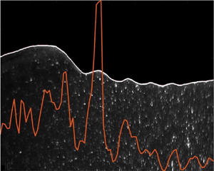
Figure 26. Dissipation rate (red curve) and vorticity field of a breaking 6 Hz wave.

Figure 27. Evolution of vorticity in the micro-breaking process: (a) $t=0.02\,{\rm s}$; (b) $t=0.04\,{\rm s}$; (c) $t=0.06\,{\rm s}$; (d) $t=0.08\,{\rm s}$.

Table 3. Experimental studies of kinematic breaking onset in the literature.

Table 4 shows the parameters for micro-breaking onset recorded in this study. It can be seen from table 4 that, as the wave shortens, the onset steepness becomes smaller, but the ratio of particle to phase speed increases. Surface tension plays a significant role in micro-breaking. The breaking type often depends on the Bond number and the wave steepness. Although breaking onsets have been studied widely, parameters for breaking waves at small scales are virtually absent in the literature. For the same Bond number and steepness in two-dimensional facilities, only parasitic capillary waves have been presented in the literature, and no breaking waves have been reported. Thus, the convergent channel coupled with added surfactant facilitates wave breaking.

Table 4. Wave parameters at onset of breaking, with added surfactant.

4.3. Energy dissipation during micro-breaking

The energy dissipation rate of a breaking 5.5 Hz wave is shown in figure 26. It is obtained using the same method as described in § 3.3. The maximum dissipation rate appears on the forward side of the crest where the primary wave crest merges into the parasitic wave. It can also be seen in figure 26 that the maximum dissipation rate occurs in the vicinity of the highest vorticity. By comparing the instantaneous dissipation rate of the parasitic waves and micro-breaking in figures 18 and 26, it can be concluded that the dissipation rate of micro-breaking is much higher than the dissipation rate of parasitic capillary waves. After breaking, the wave no longer retains its regular profile and the wave elevation decreases significantly. In the parasitic wave cases, although parasitic waves dissipate energy, the primary waves are able to maintain their wave elevation. However, the total energy dissipated through parasitic waves is comparable to the energy dissipated through the breaking process. As figures 18 and 26 only show the instantaneous energy dissipation rate, the parasitic waves persist for the entire propagation, while breaking only occurs for a shorter period of time. For the breaking cases, due to added surfactant, the parasitic waves are generally suppressed.

In figure 28, the potential and kinetic energy evolution is shown for waves with parasitic waves and waves with added surfactant (micro-breaking waves). The data are from the 6 Hz wave experiments (case 3 in table 1 and case 9 in table 4). The energy is calculated using the wave profile (potential) and velocity field (kinetic); (3.4) and (3.5) are used for this calculation. Thus the total energy of half of the wavelength is considered (shown in the figure). The energy evolution of one particular wave segment is calculated by propagating the calculation domain with the wave, at the phase speed. Here $E$ represents the instantaneous energy, $E_0$ is the initial total energy and $T$ is the wave period. The initial energy calculation does not start from the first wave near the wavemaker, but from the starting point of the laser sheet. Initially, the dissipation rate of the two waves is close, but by $t/T=0.4$, the parasitic waves are dissipating more. However, at approximately $t/T=0.95$, the breaking process starts on the waves with added surfactant, and the dissipation rate increases significantly, as shown by the solid blue curve. The figure also shows that the ratio of potential energy and kinetic energy is not $1:1$ as predicted by linear theory. In waves with surfactant, where parasitic waves are mostly absent, the initial kinetic energy contributes approximately 54 % of the total energy while the potential energy contribution is around 46 %. In the wave without surfactant but with parasitic waves, the contribution of kinetic energy increases to approximately 60 %, while the potential energy reduces to 40 %. This is different from the previous studies of waves before and during spilling or plunging breaking (Lim et al. Reference Lim, Chang, Huang and Na2015; Derakhti & Kirby Reference Derakhti and Kirby2016; Na et al. Reference Na, Chang and Lim2020). In the experiments herein, in a convergent channel, the parasitic waves experience an increase in the ratio of kinetic energy to total energy.

Figure 28. Energy evolution of parasitic waves and micro-breaking. Blue curves: waves with surfactant (breaking); red curves: waves without surfactant (parasitic); solid curves: total energy; dashed curves: kinetic energy; dotted curves: potential energy.

Figure 29 shows a comparison of the the kinetic and potential energy evolutions of parasitic waves in this study with some selected numerical results in the literature. The numerical results for $\lambda =5\,{\rm cm}$ are selected, for comparison with case 3 ($\lambda =4.85\,{\rm cm}$) in this study. It can be seen in the figure that the dissipation rate in this study is much higher than those in the numerical results. This is because the steeper parasitic waves in the convergent channel contribute stronger dissipation. Also, it is noted that in the numerical results, the ratio of potential and kinetic energy starts at 1. This is because in the numerical study at $t=0$, the parasitic waves are yet to be generated, while in the experiments, there are already parasitic waves at the beginning of the measurement. Both numerical and experimental results show higher kinetic energy than potential energy after the generation of parasitic waves. It might be more suitable to start the numerical results at around $t/T=1$ when comparing with the experimental results. It is also worth noting that the oscillation modes in the kinetic and potential energy in the numerical results are not observed in the experiments.

Figure 29. Energy evolution of waves with parasitic waves. Two numerical studies in the literature and the present experiments. In Tsai & Hung (Reference Tsai and Hung2010, figure 1f,g,h), $\lambda =5\,{\rm cm}, ka=0.28$ is selected. In Deike et al. (Reference Deike, Popinet and Melville2015, figure 8e), $Bo = 10$, $ka=0.3$ is selected. Case 3 in this study: $Bo = 8.34$, $\lambda =4.85\,{\rm cm}, ka=0.26$.

Comparison of energy evolution of small-scale breaking is shown in figure 30. Case 9 in the present study is compared with numerical results in Deike et al. (Reference Deike, Popinet and Melville2015). In case 9, the primary wave steepness $ka=0.28$. The Bond number $Bo=17.4$, while in the case from Deike et al. (Reference Deike, Popinet and Melville2015), $ka=0.45, Bo=10$. The two cases have similar Bond number, but the case in Deike et al. (Reference Deike, Popinet and Melville2015) has much higher steepness and was categorized as a spilling breaker. It can be seen in the figure that the dissipation rate of the experimental results is close to the numerical one. The kinematic energy remains higher than the potential energy in both cases.

Figure 30. Energy evolution of small-scale breaking waves. In Deike et al. (Reference Deike, Popinet and Melville2015, figure 8f), $ka=0.45, Bo=10$ is selected. Case 9 in this study, $Bo=17.4, ka=0.28$ is presented.

Two non-dimensional parameters are critical to the breaking pattern of waves: steepness $ka$ and the Bond number $Bo$. Deike et al. (Reference Deike, Popinet and Melville2015) showed a wave regime diagram with boundaries between different types of breaking waves, based on the numerical results. The figure is replotted here as figure 31. Three micro-breaking cases observed in this study are added to the diagram, shown as filled blue circles. It is noted that these micro-breaking cases are beneath the breaking boundary, in the parasitic capillary wave regime. To the best of the authors’ knowledge, no breaking waves have been reported in this regime without wind, either numerical or experimental. This is as a consequence that almost all previous numerical and experimental studies in this regime were conducted either in two-dimensions or in rectangular tanks, and the subsequent dissipation of parasitic waves prevented the breaking. Micro-breaking occurs in this study due to the increase of energy flux caused by spatial convergence.

Figure 31. Wave regime diagram. The boundaries between the wave regimes obtained numerically in Deike et al. (Reference Deike, Popinet and Melville2015, figure 7). PB: plunging breakers; SB: spilling breakers; PCW: parasitic capillary waves; NB: non-breaking gravity waves. Blue circles represent micro-breaking cases 7, 8, 9 in this study.