


1. Introduction
The swimming of flagellated micro-organisms is a timely subject, at the crossroads of active matter, hydrodynamics and biophysics. In a larger prospective, understanding the behaviour of semi-dilute to dense suspensions of active (self-propelled) particles is a central question of contemporary physics. From a theoretical standpoint, a considerable amount of work has been devoted to explain the emergence of collective behaviours (flocking, etc) in such systems.
While in low-concentration suspensions only individual motions prevail (Lauga & Powers Reference Lauga and Powers2009), when the concentration is higher than a few percent in volume, interactions between neighbouring microbes are no longer negligible. It generally consists in repulsion or self-alignment and can lead to collective behaviour like, for instance, the so-called bacterial turbulence (Dombrowski et al. Reference Dombrowski, Cisneros, Chatkaew, Goldstein and Kessler2004; Dunkel et al. Reference Dunkel, Heidenreich, Drescher, Wensink, Bär and Goldstein2013), or the spontaneous formation of flocks (Bricard et al. Reference Bricard, Caussin, Desreumaux, Dauchot and Bartolo2013) that offer striking similarities with the liquid/gas phase transition. On the experimental side, however, such a phenomenology is only observed in highly confined systems.
In a situation of intermediate concentration, typically from 0.1 to a few percent, fluctuations of concentration across the suspension induce corresponding fluctuations of the suspension effective density since a perfect density matching between micro-organisms and the surrounding fluid is seldom achieved. These density gradients in turn generate pressure gradients that drive macroscopic flows within the suspension, whose typical scale is much larger than the microbe size, a phenomenon called bioconvection (Childress, Levandowksy & Spiegel Reference Childress, Levandowksy and Spiegel1975; Kessler Reference Kessler1985; Pedley, Hill & Kessler Reference Pedley, Hill and Kessler1988; Hill, Pedley & Kessler Reference Hill, Pedley and Kessler1989; Pedley & Kessler Reference Pedley and Kessler1992; Vincent & Hill Reference Vincent and Hill1996; Bees & Hill Reference Bees and Hill1997, Reference Bees and Hill1998; Janosi, Kessler & Horvath Reference Janosi, Kessler and Horvath1998; Ghorai & Hill Reference Ghorai and Hill2005; Williams & Bees Reference Williams and Bees2011a,Reference Williams and Beesb). Such density fluctuations typically arise from the directional swimming of individual cells. Directional swimming is generally induced by taxes, i.e. the ability of micro-organisms to swim along vectorial fields (e.g. gravity, electromagnetic fields, etc.) or gradients of scalar fields (e.g. concentration of dissolved chemicals, temperature, etc.). For example, positive gravitaxis denotes the ability of some bottom-heavy microbes to swim with an average-upward motion (against the direction of gravity). The subsequent accumulation of microbes on top of the suspension can induce buoyancy-driven instabilities (Hill et al. Reference Hill, Pedley and Kessler1989; Bees & Hill Reference Bees and Hill1997, Reference Bees and Hill1998; Williams & Bees Reference Williams and Bees2011a,Reference Williams and Beesb) provided the density gradient is large enough compared with the action of diffusion and viscosity.
Therefore, the onset and magnitude of these flows are naturally ruled by a direct analog of the Rayleigh number:  $H^3 \rho _0 \beta g \Delta c/(D \eta )$, where $H$ is the depth of the suspension (in the direction of gravity), $\rho _0$ is the density of the medium in absence of the cell, $g$ is the gravity constant, $\beta =(\rho _{ref}-\rho _0)/(c_{ref}\rho _0)$ is the relative difference between cells and the surrounding fluid (where $\rho _{ref}$ is the density of a suspension at concentration $c_{ref}$), $D$ is the effective diffusion coefficient of randomly swimming micro-organisms, $\eta$ is the fluid dynamic viscosity, supposedly independent of the cell concentration, and $\Delta c$ is the magnitude of the cell density averaged finite difference. Similarly to the classical thermal convection (Birikh Reference Birikh1966), spontaneous bioconvection then occurs when the Rayleigh number is larger than a threshold value, typically of a few hundreds, as shown for various species such as the model phototactic algae Chlamydomonas reinhardtii (CR) (Harris Reference Harris2009) that is investigated in the present study. On the experimental side however, and in contrast with thermal convection, the magnitude of $\Delta c$ cannot be directly imposed nor controlled in a stationary way. Because the Rayleigh number cannot be directly imposed experimentally, it is convenient to introduce a pseudo-Rayleigh number $Ra$ based on the initial cell concentration $c_0$ that is readily imposed in experiments. This number is then rather defined as
 \begin{equation} Ra \equiv \frac{H^3 \beta \rho_0 g c_0}{D \eta}. \end{equation}
 While this definition is indeed convenient to compare experimental results and, as we shall see later, naturally arises from classical models of bioconvection, the threshold values that control the emergence of symmetry-breaking bioconvective instabilities depend on the underlying mechanism responsible for the emergence of density fluctuations. While most previous studies on bioconvection investigated the influence of a global forcing (e.g. gravity alone or coupled with directional lighting, for instance (Williams & Bees Reference Williams and Bees2011a)), a few recent experimental and numerical studies demonstrated that a thin light beam could induce efficient (photo)-bioconvection under low  $Ra$ conditions (Dervaux, Capellazzi Resta & Brunet Reference Dervaux, Capellazzi Resta and Brunet2017; Arrieta et al. Reference Arrieta, Polin, Saleta-Piersanti and Tuval2019; Ramamonjy, Dervaux & Brunet Reference Ramamonjy, Dervaux and Brunet2022). In these studies, CR accumulate around a light beam of width $w \ll H$, which in turn induces convective flows that can be as large as the container size, typically a few centimetres. This accumulation is due to the phototactic properties of the microalgae that exhibit directional swimming in the presence of a light intensity gradient. Under appropriate conditions ( $Ra \gtrsim$ 100), the accumulation of CR can also generate secondary instabilities, where axisymmetric rings of concentration propagate outwards from the beam at a well-defined velocity (Dervaux et al. Reference Dervaux, Capellazzi Resta and Brunet2017), a phenomenon attributed to a subtle coupling between phototaxis, self-generated convective flows and gyrotactic-induced flow focusing. Gyrotaxis, which will be introduced in greater detail below, is a physical effect arising from the coupling between the flow vorticity and the directional swimming of micro-organisms (Kessler Reference Kessler1985; Garcia, Rafaï & Peyla Reference Garcia, Rafaï and Peyla2013).
One of the practical interests to generate light-controlled photo-convective flows with spatiotemporal instabilities at relatively low  $Ra$ can be foreseen in mixing enhancement, which is often required for an efficient and well-distributed access to nutrients, in particular in photo-bioreactors. In seeking for a way to generate more complex flow patterns under low $Ra$ conditions, the present study investigates the situation where the light beam $w$ is comparable or slightly wider than the suspension depth $H$. In practice, three control parameters are varied: the suspension concentration $c_0$, the layer thickness $H$ and the width $w$ of the laser beam. From these quantities, we define two dimensionless numbers: the dimensionless beam width $w/H$, which was varied between 0.5 and 20 as well as the pseudo-Rayleigh number that was varied approximately between 5 and 1000. Let us note that above a critical value of the pseudo-Rayleigh number of around 1500, the cell suspension becomes globally unstable, even in the absence of a light intensity field. As mentioned above, in this case the bioconvective instability is induced only by gravitaxis (Plesset & Winet Reference Plesset and Winet1974; Childress et al. Reference Childress, Levandowksy and Spiegel1975; Dervaux et al. Reference Dervaux, Capellazzi Resta and Brunet2017).
In this paper our experiments reveal up-to-now unreported spatiotemporal dynamical regimes, where the concentration field is no longer axisymmetric, which presumably couples with the associated convective flow in a non-trivial way. We first present the experimental set-up and establish a diagram of existence of the different spatiotemporal regimes by systematically varying the beam width and the Rayleigh number. At moderate  $Ra$ and large $w/H$, the concentration field shows a drift of its centre of mass from the beam centre. At higher $Ra$ and moderate $w/H$, a dendrite-like pattern of concentration appears, with remarkable spatial periodicity in the azimuthal direction, for which we conduct a quantitative study (§ 2). In § 3 a model of bioconvection incorporating both gyrotaxis and the nonlinear phototactic response is introduced and solved numerically in two dimensions. In order to gain further insight into the physical mechanisms underlying the instabilities observed experimentally, and taking advantage of the geometry of our experimental system, a lubrication approximation is used in §§ 4 and 5 to develop an asymptotic model of bioconvection in a thin film, once again in the presence of phototaxis and gyrotaxis. In particular, the full model of bioconvection is reduced to a single nonlinear anisotropic diffusion–drift equation describing the depth-averaged cell concentration in the thin liquid layer. A physical interpretation of this equation is presented in § 6 before making a comparison between our experimental results and analytical/numerical solutions of this equation (§ 7). Finally, we summarise our findings and suggest perspectives for future studies in § 8.
2. Experimental results
2.1. Set-up
In this work we investigate the collective behaviour of a suspension of CR under heterogeneous light fields. The experimental set-up, already used in previous studies (Dervaux et al. Reference Dervaux, Capellazzi Resta and Brunet2017; Ramamonjy et al. Reference Ramamonjy, Dervaux and Brunet2022) is summarised in figure 1(a). A levelled petri dish (inclination  ${\leq }0.1^{\circ }$) is filled with a layer of thickness $H$ (typically of the order of a millimetre) of a suspension of CR at concentration $c_0$ (typically of the order of $10^6$ cell ml $^{-1}$). A radially symmetric green laser beam shines the suspension in order to create a heterogeneous light exposure (see figure 1b,c). The shape of the light beam can be approximated by a Gaussian core supplemented by an exponential tail, as shown in figure 1(d). In order to control the beam width, we add one or several diffusing layers between the laser and the petri dish while its intensity can be tuned using a pair of crossed polarisers. The diffusers only have a minor effect on the width of the Gaussian part of the light beam: the beams of figure 1(b,c) are barely distinguishable from each other. However, they significantly change the width of the exponential tail, as shown in radial profiles of figure 1(d). No difference in the cell response could be observed between polarised and non-polarised light. More details on the experimental protocol are provided in Appendix A.

Figure 1. (a) Sketch of the experimental set-up used to measure phototactic response. A petri dish contains a suspension of CR that are attracted toward a green light beam by phototaxis. A camera acquires the depth-averaged cell concentration field from above from the measurement of red light transmitted through the suspension. The experimental set-up is kept in a dark enclosure. (b,c) Images of laser beams reconstructed from their light intensity profiles. The images shown correspond to the smallest (b) and the largest beam width  $w$ (c). (d) Radial profiles of laser beams intensity for five different widths $w$, with a fixed maximum intensity of $I_{max} = 5$ W m $^{-2}$. (e) Phototactic susceptibility $\chi (I)$ versus light intensity, from (Ramamonjy et al. Reference Ramamonjy, Dervaux and Brunet2022).
At time  $t = 0$, the laser is switched on. Because of their phototactic properties, CR cells move toward the light beam where they accumulate over time and form a well-defined concentration pattern that can be, as we shall detail below, stationary, periodic or continuously growing over the time scale of an experiment, roughly 90 min. The algae drift toward the light source with a velocity $v_{drift}$ proportional to the light intensity gradient: $v_{drift}=\chi (I)\boldsymbol {\nabla }I$. The proportionality coefficient, $\chi (I)$, is called the phototactic susceptibility and has been demonstrated to be a highly nonlinear function of the light intensity (Ramamonjy et al. Reference Ramamonjy, Dervaux and Brunet2022); see figure 1(e).
Because CR cells exhibit a negative phototactic response ( $\chi (I)<0$) above a critical light intensity $I_{c} \simeq 100$ W m $^{-2}$, i.e. cells swimming away from the light source, the maximum light intensity was kept at a constant value of 5 W m $^{-2}$ in all experiments in order to elicit only the positive phototactic response ( $\chi (I)>0$). Recent results revealed that the maximum sensitivity of the phototactic response of CR to light intensity gradient was found at a very low light intensity (Ramamonjy et al. Reference Ramamonjy, Dervaux and Brunet2022), typically around $I_{th} \simeq 10^{-3}$ W m $^{-2}$, a value also close to the detection threshold. Furthermore, the susceptibility $\chi (I)$ decreases monotonically with increasing intensity $I$ before changing sign (i.e. CR cells move away from the light source) at $I_{c}$. Let us note that a qualitatively similar behaviour has also been reported for Euglena gracilis (Giometto et al. Reference Giometto, Altermatt, Maritan, Stocker and Rinaldo2015). Consistently with the measured susceptibility $\chi (I)$, we define the width $w$ of the light beam as the distance from the centre of the beam where the light intensity falls below an arbitrary threshold of $0.5\,\%$ of the maximum light intensity (i.e. around $5\times 10^{-2}$ W m $^{-2}$). This highly nonlinear susceptibility suggests that a significant – and possibly dominant – contribution of the phototactic flux of algae should occur along the tail of the light beam, i.e. in the region of relatively weak intensity where $I$ is slightly higher than $I_{th}$. Hence, besides the pseudo-Rayleigh number $Ra$, another presumably important control parameter is the width of the light beam. In the present study, both parameters are varied within a large range in order to better understand the crossed influence of these quantities.
2.2. Phase diagram
In this section we classify the various patterns observed in the  $\sim$100 independent conducted experiments. Four main patterns are identified and their domain of existence in the parameter space are represented in figure 2. At relatively small beam width and pseudo-Rayleigh number, only round patterns are observed. They are stationary and circular and closely follow the light beam (figure 2a and pale blue region in figure 2f). As we already showed in a previous work (Dervaux et al. Reference Dervaux, Capellazzi Resta and Brunet2017), when the pseudo-Rayleigh number is increased at low $w/H$, wave emission occurs: round patterns become unstable and stationarity is lost (figure 2b and pale pink region in figure 2f). While they remain approximately axisymmetric, waves of high algae concentration are periodically emitted. At a larger relative beam width $w/H$, a very different short wavelength instability is found, also above a critical threshold in Rayleigh number. These patterns consist of periodic thin dendrites that grow radially and exhibit splitting until a final state is reached (figure 2c and pale green region in figure 2f). In this dendrite instability the orthoradial invariance is lost but we can anyway extract stationary time-averaged physical quantities from the depth-averaged concentration field $\bar {c}(r,\theta,t)$. Finally, at intermediate Rayleigh number and large enough $w/H$ ratio, a fingering instability with directional growth is observed. In this regime a single finger (or bulge) grows from the initial – and transient – circular cell aggregate (figure 2d). Note that we also observe a mixed state in which the fingering directional growth and the dendrite instability occur together (figure 2e).

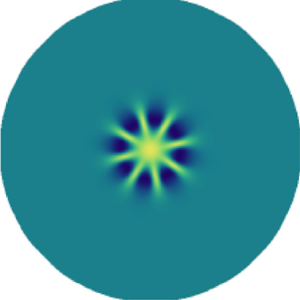
Figure 2. (a–e) Cell concentration fields imaged from the top view of the different types of patterns observed in photo-bioconvection experiments. Images are centred around the light beam. Colourmap with low concentrations in dark blue, high concentrations in dark red and maximum brightness for intermediate concentrations. The three main patterns are round, waves and dendrites. (a) Stationary round pattern. (b) Waves of concentration ‘rings’ propagating radially from the centre to the periphery. (c) Dendrite-like pattern with branches of high concentration continuously splitting and merging, and a stationary radial extension. (d,e) Unsteady directional growth (or fingering instability) from a initially round pattern (d) and from dendrites (e). (f) Occurrences of the different pattern types are plotted in a phase diagram with pseudo-Rayleigh number  $Ra$ and relative beam width $w/H$ as control parameters. Boundaries are a guide for the eye to delimit the domains of existence of round, waves and dendrites patterns that are respectively coloured in pale blue, green and violet.
2.3. Global properties of the cell patterns
Two typical experiments are shown in panels (a) to (g) of figure 3 and illustrate how an initially homogeneous culture subjected to the light beam (figure 3a) becomes progressively inhomogenous and ultimately forms spatially structured patterns. At a large beam width and high Rayleigh number (figure 3e–g), transient dots are sometimes observed (figure 3e). They are millimetre-sized structures that move toward the centre of the beam and merge to form the final pattern. Next, let us focus on the global properties of the cell concentration patterns: in figure 3 we report the maximum cell concentration and the pattern size as a function of both the Rayleigh number and the beam width. As shown in figure 3(h), the pattern size  $R_{1/2}$ is defined as the distance from the centre of the beam where the cell concentration is halfway (median value) between the maximum concentration $c_{max}$ and the initial concentration $c_0$: $c_{1/2} (R_{1/2}) = (c_0 + c_{max})/2$. Experiments that exhibit a fingering instability are excluded from this analysis since this quantity is then not well defined. Let us note that the maximum cell concentration is always located at the centre of the beam. In panels (i) and (j) of figure 3, it can be seen that the maximum cell concentration and pattern radius in a typical experiment increase monotonically in time before reaching a saturation value after $\sim$1 h. The stationary values (or the average value for time-dependent periodic wave patterns) are recorded in panels (k) and (l) of figure 3 as a function of both the Rayleigh number and the beam width $R_{1/2}$. While the maximum cell concentration strongly decreases when the Rayleigh number is increased, no significant dependence of $c_{max}$ on the beam size could be detected. The pattern size on the other hand strongly increases with both the beam size and the Rayleigh number.

Figure 3. (a–g) Concentration pattern in green pixel level, showing the time evolution from an initial homogeneous culture (a), for two values of beam width  $w = 2.7$ mm (snapshots b–d) and $w = 7.5$ mm (snapshots e–g). (h) Stationary cell concentration radial profile ( $w = 7.5$) and definition of median concentration $c_{1/2} = (c_0 + c_{max})/2$ and corresponding radius $R_{1/2}$ (also represented in panel g). (i,j) Time evolution of $c_{max}$ and $R_{1/2}$ (same conditions as in panel h). (k,l) Normalised maximum concentration $c_{max}/c_0$ and pattern size $R_{1/2}$ versus pseudo-Rayleigh number $Ra$ for different beam widths $w$. Each point corresponds to a single experiment. Error bars take into account both the accuracy of the local cell concentration measurements by red light transmission, and the variability when averaging cell concentration profiles over time and along $\theta = [0; 2{\rm \pi} ]$. Lines: theoretical predictions from the asymptotic model, obtained from (7.2) with $A = 26 \pm 6$ and $\alpha _0 = (1.5 \pm 0.2) \times 10^{-4}$.
2.4. The dendrite pattern
The so-called dendrites regime denotes a concentration field that self-organises into a pattern of branches, see figure 2(c) and shown as green star symbols in the phase diagram (figure 2f). It is found to occur at a rather large beam width (it does not appear for the smallest value of  $w = 2.7$ mm), and it requires a relatively large pseudo-Rayleigh number. The phase diagram indicates that the critical Rayleigh number above which the dendrite pattern appears depends on the relative beam width $w/H$.
While the centre of mass of this pattern roughly remains at the centre of the laser spot, the depth-averaged concentration  $\bar {c}(r,\theta,t)$ is no longer axisymmetric. The formation of dendrite patterns follows a transient regime where spots of larger concentration form in the suspension within the first tens of minutes (figures 3e and 4b) after the laser light is turned on. This pattern of dots, appearing in a region around the light beam of area increasing with both $w$ and $Ra$, is reminiscent of spontaneous bioconvective instabilities that originate from the upward swimming of micro-organisms (Bees & Hill Reference Bees and Hill1997; Williams & Bees Reference Williams and Bees2011b). During this transient stage, the maximum cell concentration near the centre increases in time while the overall concentration field self-organises in radially growing branches of relatively high concentration (figure 4c). The evolution of branches with time exhibits a complex dynamics involving the merging and splitting of dendrites. This dynamics is shown with a kymograph depicting the time evolution of the angular concentration profiles at a fixed distance from the beam centre (figure 4e). Despite these dynamical events, the average spacing between branches remains fairly well defined. The pattern eventually reaches a stationary state of maximum radial extension (figure 4d) from which we measured the spacing between branches (see Appendix A). The normalised orthoradial wavelength $\lambda /H$ is plotted versus $Ra$ for different $w$ in figure 4(f). Error bars are mainly a consequence of the circular geometry that prevents a strictly constant interbranch distance. Although the domain of existence of dendrites patterns in the phase diagram depends on $w$, no effect of $w$ could be noticed on $\lambda$. Also in the range of the error bars, the value of the normalised wavelength, measured as $\lambda / H = 0.63 \pm 0.08$, is largely independent of $Ra$.
$Ra$.

Figure 4. (a–d) Cell concentration field imaged from the top view at different times during a typical experiment showing the formation of dendrites. The light beam at the centre is turned on at  $t = 0$. From an homogeneous cell concentration field, (a) aggregate dots of intermediate concentrations move towards the centre (b) where branches split and grow with increasing concentration at the centre (c) before reaching a steady state (d). (e) For the same experiment, kymograph of the cell concentration as a function of time and the angular coordinate $\theta$ at a fixed distance 5 mm from the beam centre. Arrows show splitting events while merging events are circled. Here $Ra = 1100$ ( $H = 0.51$ mm, $c_0 = 2.6\times 10^6$ cells mL $^{-1}$), $w = 20$ mm. (f) Relative averaged wavelength of the dendrite pattern as a function of the pseudo-Rayleigh number.
2.5. Directional growth or budding instability
The regime of directional growth denotes a situation, observed at high beam width ( $w/H > 1$), where the concentration field progressively and continuously destabilises into a unique finger (or bud) drifting from the centre of the beam; see figure 2(e). This directional growth occurs either from initially round patterns at low pseudo-Rayleigh number $Ra$, or mixed with dendrites at higher $Ra$. In both case, the same phenomenology is observed. The cell concentration pattern is initially centred but gets destabilised, as a finger grows in a given direction while the pattern (and, thus, part of the algal biomass) remains centred around the light beam. For $w/H >$ 1, directional growth occurred indifferently along the whole range of $Ra$. Still, based on our repeated systematic experimental runs, it is more likely to occur for low to intermediate values of $Ra$ (typically below 300).
Figure 5 summarises the main findings concerning the regime of directional growth and, in particular, the time evolution of the pattern. In experiments the concentration field pattern first evolves into a pseudo-elliptical shape; see panels (a)–(c) of figure 5. This ellipse is delimited by the location of the isoconcentration line  $c_{max}/2$, from which we extracted the minor and major axes lengths $2a$ and $2b$, the aspect ratio $a/b$ as well as its growth rate $\nu$ (figure 5d,e). The quantity $\nu$, which has the dimension of an inverse of time, is extracted during the late phase as the length of the minor axis $2b$ reaches a constant value while the major axis $2a$ continues to grow. The values of $\nu$ are plotted versus $Ra$ in figure 5(f) for all situations where such a quantitative extraction was possible, with and without dendrites. Since the typical pattern size is roughly $\sim$10 mm, this corresponds to physical drift velocities of the order of a few $\mathrm {\mu }$m s $^{-1}$. This is much smaller than the velocity of the primary convection roll that typically exceeds 100 $\mathrm {\mu }$m s $^{-1}$ with these experimental conditions (Dervaux et al. Reference Dervaux, Capellazzi Resta and Brunet2017). We observed a decrease of the anisotropy growth rate with $Ra$, consistent with our finding that the directional growth instability is favoured at low to moderate pseudo-Rayleigh numbers.

Figure 5. (a–c) Concentration field at different times during an experiment showing directional growth. Cells accumulate around the light beam (a), reaching a maximum concentration at the centre (b). The pattern eventually grows toward a well-defined direction  $\theta _0$ away from the centre (here towards the left of the image) with an aspect ratio quantified by its growth rate $\nu > 0$. (c–f) The region for which $c(r, \theta, t) > c_{max}(t)/2$ can be described by an ellipse of orientation $\theta _0$ and of major and minor axes lengths $2a$ and $2b$. The evolution of axes lengths (d) and aspect ratio (e) with time allows us to quantify the kinetics of directional growth. For $t > t_1$, the slope estimate and standard deviation of a linear fit of the aspect ratio gives an anisotropy growth rate $\nu = (7.2 \pm 0.6)\times 10^{-3}$ min $^{-1}$. Here $Ra = 95$ ( $H = 0.24$ mm, $c_0 = 2.2 \times 10^6$ cells mL $^{-1}$) and $w = 7.5$ mm. (f) Anisotropy growth rate showing directional growth versus pseudo-Rayleigh number. Each point corresponds to a single directional growth event. (g) Statistics of directional growth events in intervals of pseudo-Rayleigh number for beam widths $w \ge 5.0$ mm. Labels ‘unstable’ and ‘stable’ respectively correspond to the occurrence and non-occurrence of directional growth. (h,i) Experiments of directional growth of photo-bioconvection patterns with a slight inclination of the suspension. (h) Principle of the tilting experiment. An inclination $0.1 \pm 0.05^{\circ } \le \alpha \le 1.0 \pm 0.05^{\circ }$ of the petri dish with respect to the horizontal is imposed and induces directional growth towards the lower side of the petri dish. (i) Anisotropy growth rates as a function of the petri dish inclination for different beam widths $w$ at fixed pseudo-Rayleigh number $Ra = 140$. The numbers in the legend indicate the thickness of the diffusing layer. Here 1, 2 and 4 correspond to beam widths $w$ of $5$,
$5$,  $7.5$ and $20$ mm, respectively.
Figure 5(g) plots the number of occurrences of stable (symmetric pattern, without directional growth) and unstable (directional growth) situations for different intervals of  $Ra$, clearly showing that the instability is more likely to appear at relatively low $Ra$.
$Ra$.
To better apprehend the underlying mechanisms from which directional growth originates, we carried out experiments by slightly tilting the petri dish, with an angle  $\alpha$ from the horizontal, as sketched in figure 5(h), in order to check whether or not the directional growth could be induced by minor imperfections of the dish horizontality. These experiments were operated at fixed $Ra = 140$ with three beam widths $w = 5.0$, 7.5 and 20 mm. We found that directional growth was indeed promoted by such a slight inclination of the dish. Patterns grew towards the lower side of the petri dish, i.e. the side where the layer thickness is the largest. Furthermore, we measured their anisotropy growth rate $\nu$ for various $\alpha$. For $w = 5.0$ mm, we measured $\nu < 4.0 \times 10^{-3}$ min $^{-1}$. For $w = 7.5$ and 20 mm, $\nu$ increased from $1.5 \times 10^{-2}$ to $1.7 \times 10^{-1}$ min $^{-1}$ for $\alpha$ increasing from 0.1 to 1.0 $^{\circ }$. The value of $1.5 \times 10^{-2}$ min $^{-1}$ for $\alpha = 0.1 \pm 0.05^{\circ }$ is indeed close to the upper limit of the values of anisotropy growth rate measured with a petri dish levelled with the best possible accuracy. This is consistent with a possible departure from horizontality of angle ${\lesssim } 0.1^{\circ }$ in the main experiments. To summarise, although the mechanism behind this instability is not fully pinpointed at this stage, the directional growth instability reveals a striking increase of the system sensitivity to any slight asymmetry when the beam gets larger.
3. Model
3.1. Fundamental equations
Let us now write the general equations describing the collective behaviour of a suspension of CR cells in the presence of a heterogeneous light field. We shall use a fairly general continuum deterministic model of bioconvection with gyrotaxis (Childress et al. Reference Childress, Levandowksy and Spiegel1975; Pedley & Kessler Reference Pedley and Kessler1990, Reference Pedley and Kessler1992), supplemented by an equation of the Keller–Segel form (Keller & Segel Reference Keller and Segel1971) describing the conservation of the total number of cells in the presence of advection, taxis and diffusion:
 \begin{equation}\left.\begin{array}{c@{}} \text{Incompressibility},\quad \boldsymbol{\nabla} \boldsymbol{\cdot} \boldsymbol{v} = 0; \\ \text{Momentum conservation},\quad \rho_0 \dfrac{{\rm D}\boldsymbol{v}}{{\rm D}t} = \eta \Delta \boldsymbol{v} - \boldsymbol{\nabla} p - \rho_0 \beta c g \boldsymbol{e}_z; \\ \text{Gyrotaxis},\quad \dfrac{\partial \boldsymbol{q}}{\partial t} = \dfrac{1}{2B} [ \boldsymbol{e}_{p} - (\boldsymbol{e}_{p} \boldsymbol{\cdot} \boldsymbol{q}) \boldsymbol{q} ] + \dfrac{1}{2} \boldsymbol{\omega} \times \boldsymbol{q}; \\ \text{Cell conservation},\quad \dfrac{\partial c}{\partial t} = \boldsymbol{\nabla} \boldsymbol{\cdot} (\underbrace{D \boldsymbol{\nabla} c}_{diffusion} - \underbrace{c |v_{drift}| \boldsymbol{q}}_{{drift \, due \, to \, taxis}} - \underbrace{c \boldsymbol{v}}_{advection}).\end{array}\right\} \end{equation}
Here  $\boldsymbol {\omega } = \boldsymbol {\nabla } \times \boldsymbol {v}$ is the flow vorticity associated with the flow field $\boldsymbol {v}$. The vector $\boldsymbol {q}$ is the average orientation of the swimming micro-organisms. Let us note that the Boussinesq approximation (Tritton Reference Tritton1988) has been used to obtain the first two equations of (3.1). As a reminder, the quantities $\rho _0$ and $\eta$ respectively stand for the density and viscosity of the ambient medium. The coefficient $\beta$ stands for the normalised density mismatch between microbes and the ambient medium, and $g$ stands for the gravity constant. The quantity $D$ is the diffusion coefficient of the microbes; its value is $0.85\pm 0.15 \times 10^{-7}$ m $^2$ s $^{-1}$ for CR (Polin et al. Reference Polin, Tuval, Drescher, Gollub and Goldstein2009; Dervaux et al. Reference Dervaux, Capellazzi Resta and Brunet2017). We assume that $D$ and $\eta$ are independent of the local concentration $c$, although such a dependence may become significant at larger concentrations than those used in our experiments (Rafaï, Jibuti & Peyla Reference Rafaï, Jibuti and Peyla2010; Garcia et al. Reference Garcia, Berti, Peyla and Rafaï2011). The unitary vector $\boldsymbol {e}_{p}$ is the preferred swimming orientation of the micro-organisms and should arise from a combination of factors, as discussed below. The parameter $B$ is interpreted as the typical time scale for the mean swimming orientation to return to $\boldsymbol {e}_{p}$ when the flow is suddenly stopped ( $\boldsymbol {\omega } = \boldsymbol {0}$) (Durham, Climent & Stocker Reference Durham, Climent and Stocker2011). The phototaxis-induced drift velocity is denoted as $v_{drift}$. Cell growth is neglected in the cell conservation equation since the typical time scale of an experiment ( $\sim$1 h) is much smaller than the typical time scale of the population doubling time within our experimental set-up ( $\sim$10 h).
3.2. Structure of the primary convective roll
Let us first show that the formation of the primary instability associated with symmetric stable states can be addressed with the continuum model for bioconvection recalled above without including gyrotaxis. We only consider a phototactic drift that steers cells along the imposed light intensity gradient  ${\partial I}/{\partial r}$, where in the absence of gyrotaxis, cells are strictly oriented, on average, along their preferential orientation $\boldsymbol {e}_{p}$,
 \begin{equation} \left.\begin{array}{c@{}} |v_{drift}| = \left|\chi \dfrac{\partial I}{\partial r}\right|,\\ \boldsymbol{q} = \boldsymbol{e}_{p} \quad \text{and} \quad \boldsymbol{e}_{p} = \operatorname{sign} \left(\chi \dfrac{\partial I}{\partial r} \right) \boldsymbol{e}_r. \end{array}\right\} \end{equation}
 The nonlinear system of (3.1) restricted to the ( $\boldsymbol {e}_r,\boldsymbol {e}_z$) plane (i.e. a radial cross-section of the petri dish) and under the conditions (3.2) describes the evolution of four scalar fields (pressure $p$, concentration $c$, velocity $\boldsymbol {v}$ in ( $\boldsymbol {e}_r$, $\boldsymbol {e}_z$)). They can be solved numerically with the green light intensity radial profile $I(r)$ used in the experiments as an input, together with the nonlinear phototactic response $\chi (I)$ presented in figure 1(e). An example of such a numerical resolution with the commercial software Comsol is presented in figure 6.

Figure 6. (a) The axisymmetry enables us to work within a cross-section in a vertical ( $\boldsymbol {e}_r,\boldsymbol {e}_z$) plane and to reconstruct the three-dimensional fields by revolution around the vertical axis. (b) Side view of the stationary cell concentration field. The colourmap brightness increases in steps from white for low concentration to black for high concentration. Contour lines are isocell concentrations. (c) Radial profile of the depth-averaged scaled concentration $c/c_0$. (d) Details of the streamlines of the principal toroidal convective roll near the light source. The second counter-rotating toroidal roll can be seen further away from the centre of the light source. Red portions of the streamlines correspond to high velocities and blue portions correspond to low velocities. (e) Side view of the stationary velocity field. White arrows: local velocity vectors. The colourmap brightness increases from blue for low velocity to yellow for high velocity. (f) Vertical profile of the radial velocity at a fixed distance away from the centre (corresponding to the dashed red line in panel e).
The formation of the main toroidal flow structure is recovered. Numerical simulations give access to data that cannot be measured in the experiments: data of the cells concentration field along the suspension depth (figure 6b) and spatial profiles of the velocity field (figure 6d–f). The toroidal structure of the primary convection roll is shown in figure 6(d). Due to the density mismatch between the microbes and the ambient medium, the flow is directed downward at the centre of the light source and, as a result, the cell concentration field is pushed towards the bottom. As illustrated in panels (a)–(c) of figure 7, this effect is enhanced at high Rayleigh number and the magnitude of the flow velocity increases with the Rayleigh number. When  $Ra$ is low on the other hand, the cell concentration is almost constant across the thickness of the suspension (figure 7a). Far enough from the centre, the vertical velocity vanishes and the flow is almost horizontal (figure 6e).

Figure 7. The magnitude of convection is controlled by three values of the pseudo-Rayleigh number. From top to bottom: 0.1, 1 and 100. The magnitude of gyrotaxis is controlled by two values of the gyrotactic time scale. On the left column,  $B = 0$ s corresponds to the case without gyrotaxis; on the right column, $B = 1$ s. Contours lines show isocell concentration lines.
The 2-D model above without gyrotaxis is stable within the range of parameters explored in the experiments. In a previous study (Dervaux et al. Reference Dervaux, Capellazzi Resta and Brunet2017), it was found that waves emission could be reproduced in 2-D numerical simulations by introducing gyrotaxis and a deviation of the cells orientation with respect to their preferential direction  $\boldsymbol {q} \neq \operatorname {sign} (\chi ({\partial I}/{\partial r})) \boldsymbol {e}_r$. While gyrotaxis only has a weak effect on both the fluid flow and the depth-integrated cell concentration field, it does impact significantly the repartition of a cell across the thickness of the suspension, as seen in panels (d)–(f) of figure 7. Qualitatively, in the presence of gyrotaxis, the dense layer of cells induced by the primary convective roll is slightly shifted above the bottom of the petri dish. More precisely, the dense layer is located around the local maximum of the flow velocity (see panel f of figure 7). Because this cell-rich layer has a higher density than the cell-poor layer below, it eventually undergoes a buoyancy-driven instability above a critical $Ra$, as illustrated in figure 8. Because this secondary instability is advected by the primary convective roll, it manifests itself as rings of high concentration propagating outward from the centre of the petri dish. The wave velocities predicted by these numerical simulations were found to be in good agreement with experimental results (Dervaux et al. Reference Dervaux, Capellazzi Resta and Brunet2017). Best fits to experimental cell concentration profiles led to an estimate of the time constant $B = 1.2 \pm 0.2$ s, in agreement with previous models (Williams & Bees Reference Williams and Bees2011a; Garcia et al. Reference Garcia, Rafaï and Peyla2013).

Figure 8. Side views of the cell concentration fields obtained in 2-D numerical simulations with gyrotaxis. Contours lines show isocell concentration lines. (a) In the presence of gyrotaxis there is a gap between the cells dense layer in the lower part of the suspension and the bottom of the petri dish. (b) Later, waves are emitted. The dense layer is buoyantly unstable and breaks into clusters of high cell concentration advected by the flow. Here,  $Ra = 125$ ( $H = 2.5$ mm and $c_0 = 1.8 \times 10^6$ cells mL $^{-1}$), $w = 2.7$ mm. The image is adapted from Dervaux et al. (Reference Dervaux, Capellazzi Resta and Brunet2017).
4. Hypothesis for the development of the asymptotic model
Numerical simulations restricted to the ( $\boldsymbol {e}_r,\boldsymbol {e}_z$) plane cannot reproduce the breaking of axisymmetry observed in dendrites or in directional growth. Still, attempting a numerical computation of a full tridimensional model with gyrotaxis and nonlinear phototaxis would require heavy code optimisation and/or numerical resources to explore the phase space. In order to make further progress, we shall take advantage of the fact that our experiments are carried out in a thin-layer geometry $H \ll L$. In all generality, this horizontal scale $L$ in our experimental set-up can be related to either the typical lateral scale of the primary convective roll (which is typically of the order of a few centimetres, see Dervaux et al. Reference Dervaux, Capellazzi Resta and Brunet2017) or to the effective width of the beam. Because of the very high sensitivity of the phototactic effect, the effective width of the beam (where the light intensity is larger than $10^{-3}$ W m $^{-2}$) is in the range $\sim$1–5 cm, as seen in figure 1. Consequently, either scale is significantly larger than the liquid height $H$. We will therefore choose to simplify the model by developing an asymptotic model, adapted to describe the limit $H/L \ll 1$, which is somewhat similar to the lubrication framework in viscous-driven thin film flows (Reynolds Reference Reynolds1886). As we shall see, this approach, together with additional simplifying hypotheses that we introduce in this section, allows us to reduce the systems of vectorial equation shown above to a single nonlinear partial differential equation describing a single scalar field: the depth-averaged cell concentration in the suspension defined as $\bar {c}(r,\theta,t) = ({1}/{H}))\int _{0}^{H} c(r,\theta,z,t) \,\textrm {d}z$.
4.1. Dimensionless equations
We first rewrite in a dimensionless form the general equations (3.1) that describe the spatiotemporal evolution of the flow velocity, pressure, concentration and orientation fields. The thin film approximation will be exploited later and we first scale all lengths by the liquid height  $H$, time by the diffusion time scale $H^2/D$, concentrations by the global cell concentration $c_0$, velocities by $D/H$ and pressure by $\eta D/H^2$. To simplify the writing, we keep the same notations for both dimensioned and dimensionless space–time coordinates ( $r,\theta,z,t$), fields ( $\boldsymbol {v}, c, p, \boldsymbol {\omega }$) and operators ( ${\partial }/{\partial t}, {\textrm {D}}/{\textrm {D}t}, \boldsymbol {\nabla }, \Delta$). Dimensionless equations take the following form:
 $$\begin{gather} \text{Incompressibility},\quad \boldsymbol{\nabla} \boldsymbol{\cdot} \boldsymbol{v} = 0; \end{gather}$$
 $$\begin{gather}\text{Momentum conservation},\quad \frac{1}{S_{c}} \frac{{\rm D}\boldsymbol{v}}{{\rm D}t} = \Delta \boldsymbol{v} - \boldsymbol{\nabla} p - (Ra.c) \boldsymbol{e}_z; \end{gather}$$
 $$\begin{gather}\text{Cell conservation},\quad \dfrac{\partial c}{\partial t} = \boldsymbol{\nabla} \boldsymbol{\cdot} \boldsymbol{\mathcal{J}} \text{ with } \boldsymbol{\mathcal{J}} = \boldsymbol{\nabla} c - |\mathcal{T}_{drift}| c \boldsymbol{q} - c \boldsymbol{v}; \end{gather}$$
 $$\begin{gather}\text{Gyrotaxis},\quad {G_{y}} \dfrac{\partial \boldsymbol{q}}{\partial t} = \frac{1}{2}[\boldsymbol{e}_{p} - (\boldsymbol{e}_{p} \boldsymbol{\cdot} \boldsymbol{q}) \boldsymbol{q}] + \frac{1}{2}{G_{y}} (\boldsymbol{\omega} \times \boldsymbol{q}). \end{gather}$$
They reveal that in this model the system is governed by the following dimensionless numbers:
 \begin{equation} \left.\begin{array}{c@{}} \text{Pseudo-Rayleigh number,}\quad Ra = \dfrac{\rho_0 g \beta H^3 c_0}{D \eta}; \\ \text{Drift number,}\quad \mathcal{T}_{drift} = \dfrac{v_{drift} H}{D}; \\ \text{Gyrotactic number,}\quad {G_{y}} = \dfrac{BD}{H^2}; \\ \text{Schmidt number,}\quad S_{c} = \dfrac{\eta}{\rho_0 D}. \end{array}\right\} \end{equation}
 We already defined the pseudo-Rayleigh number  $Ra$ as the ratio of the time scale of diffusion to the time scale of convection. We see here that it quantifies the coupling of the velocity $\boldsymbol {v}$ and pressure fields $p$ with the concentration field $c$. The drift number $\mathcal {T}_{drift}$ compares the ratio of the time scale of diffusion to the time scale of the cells phototactic-induced drift. It increases as the cells swimming is more biased. The gyrotactic number ${G_{y}}$ compares the time scale of reorientation by shear stress to the time scale of diffusion. It is alone hard to relate to any physical effect because the algae reorientation time scale $B$ is usually compared with a characteristic time scale of the flow. Later, we will in fact see that, indeed, the gyrotactic effect is controlled by the product ${G_{y}} Ra$ that compares the time scale of reorientation to the time scale of convection. Finally, the Schmidt number $S_{c}$ is the ratio between momentum and cell diffusivities.
4.2. Effective drifts
In the dimensionless cell conservation (4.3) and gyrotaxis (4.4) equations, we need to specify the drift term and the orientation vectors. We consider two drifts: a phototactic drift due to the light intensity gradient of the preferential radial direction and an additional drift of preferential vertical direction. We shall discuss the origin of this vertical drift later in this section. We thus replace the generic single drift term with two drifts terms and make the hypothesis that they are additive. Each drift term has its own dimensionless drift velocity and orientation unit vector,
 \begin{equation} |\mathcal{T}_{drift}| c \boldsymbol{q} \rightarrow |\mathcal{T}_{{\parallel}}| c \boldsymbol{q}_{{\parallel}} + |\mathcal{T}_{\bot}| c \boldsymbol{q}_{\bot}. \end{equation}
 The dimensionless phototactic drift number  $\mathcal {T}_{\parallel }$ is space dependent via the light intensity gradient and the dependence of $\chi (I)$ of the light intensity. For simplicity, the second term $\mathcal {T}_{\bot }$ is assumed not to depend either on space or on time. We shall obtain its value from comparison of the model with experimental results. We have
 \begin{equation} \mathcal{T}_{{\parallel}}(r) = \chi(I(r)) \dfrac{\partial I}{\partial r}(r) \frac{H}{D} \quad \text{and} \quad \mathcal{T}_{\bot} = \frac{v_{\bot}H}{D}. \end{equation}
Here  $\boldsymbol {q}_{\parallel }$ and $\boldsymbol {q}_{\bot }$ are respectively the radial and vertical vectors in the absence of flow. However, it is essential to figure out that in the presence of complex flows (i.e. when the symmetry of the primary toroidal flow has been broken), they can have non-zero $\theta$ components due to gyrotaxis. Parameter $q_{\bot, \theta }$ originates from the $r$ component of the vorticity acting on the vertical drift whereas $q_{\parallel, \theta }$ originates from the $z$ component of the vorticity acting on the radial drift. To further simplify the analysis, we write those $\theta$ components as perturbations around known preferential horizontal and vertical orientations. Thus, the radial and vertical components are known and we have
 \begin{equation} \left.\begin{array}{c@{}} \boldsymbol{q}_{{\parallel}} = \operatorname{sign} (\mathcal{T}_{{\parallel}}) \boldsymbol{e}_r + q_{{\parallel}, \theta} \boldsymbol{e}_{\theta}, \quad |q_{{\parallel}, \theta}| \ll 1,\\ \boldsymbol{q}_{\bot} = \operatorname{sign} (\mathcal{T}_{\bot}) \boldsymbol{e}_z + q_{\bot, \theta} \boldsymbol{e}_{\theta}, \quad |q_{\bot, \theta}| \ll 1. \end{array}\right\} \end{equation}
 In the perturbative limit where  $|q_{\parallel, \theta }|,|q_{\bot, \theta }| \ll 1$, $\boldsymbol {q}_{\parallel }$ and $\boldsymbol {q}_{\bot }$ are quasi-unit vectors. Finally, we construct a total unit orientation vector $\boldsymbol {q}_{tot}$ on which to apply the gyrotaxis equation as the weighted sum of the two orientations unit vectors $\boldsymbol {q}_{\parallel }$ and $\boldsymbol {q}_{\bot }$:
 \begin{equation} \boldsymbol{q}_{tot} = \frac{|\mathcal{T}_{{\parallel}}|}{\mathcal{T}} \boldsymbol{q}_{{\parallel}} + \frac{|\mathcal{T}_{\bot}|}{\mathcal{T}} \boldsymbol{q}_{\bot} \quad \text{with}\ \mathcal{T} = \sqrt{\mathcal{T}_{\bot}^2+\mathcal{T}_{{\parallel}}^2}. \end{equation}
 By construction, we have a similar expression for the total preferential orientation  $\boldsymbol {e}_{p,tot}$ appearing in the gyrotactic equation (4.4). Then $\boldsymbol {q}_{tot}$ can also be rewritten with a perturbation on $\boldsymbol {e}_{p,tot}$. We have
 $$\begin{gather} \boldsymbol{e}_{p,tot} = \frac{|\mathcal{T}_{{\parallel}}|}{\mathcal{T}} \operatorname{sign}(\mathcal{T}_{{\parallel}}) \boldsymbol{e}_r + \frac{|\mathcal{T}_{\bot}|}{\mathcal{T}} \operatorname{sign}(\mathcal{T}_{\bot}) \boldsymbol{e}_z, \end{gather}$$
 $$\begin{gather}\boldsymbol{q}_{tot} = \boldsymbol{e}_{p,tot} + \underbrace{q_{tot,\theta}}_{|q_{tot,\theta}| \ll 1} \boldsymbol{e}_{\theta} \quad \text{with}\ q_{tot,\theta} = \frac{|\mathcal{T}_{{\parallel}}|}{\mathcal{T}} q_{{\parallel}, \theta} + \frac{|\mathcal{T}_{\bot}|}{\mathcal{T}} q_{\bot, \theta}. \end{gather}$$
 Note that such an additive decomposition for the total preferential orientation  $\boldsymbol {e}_{p,tot}$ has already been used in the literature (Williams & Bees Reference Williams and Bees2011a). In addition, we restrict ourselves to the perturbative limit ( $|q_{tot,\theta }| \ll 1$) where nonlinear effects, which may arise from the nonlinearity of the gyrotactic equation, can be neglected.
4.3. Time scales of the problem
Additional simplifications can be obtained by evaluating the characteristic time scales involved in the problem. The diffusion time scale is the longest time scale in the problem with  ${H^2}/{D} \gtrsim 10$ s with $H \gtrsim 1$ mm. The viscous time scale is ${H^2 \rho _0}/{\eta } \gtrsim 1$ s. Finally, the time scale for the gyrotactic reorientation is $B$
$B$  $\sim$1 s. The respective ratios of the viscous and gyrotactic reorientation time scales over the diffusion time scale are thus $S_{c} \sim 10$, ${G_{y}} \lesssim 0.1$.
We can thus drop the time-derivative terms in both the flow and pressure fields equation (4.2) as well as in the gyrotaxis equation (4.4). In other words, we consider that the pressure  $p$, velocity $\boldsymbol {v}$ and orientation fields $\boldsymbol {q}_{\parallel }, \boldsymbol {q}_{\bot }, \boldsymbol {q}_{tot}$ instantaneously adjust to the slowly varying concentration field $c$.
$c$.
At this stage, we can rewrite the dimensionless equations as
 $$\begin{gather} \text{Incompressibility},\quad \boldsymbol{\nabla} \boldsymbol{\cdot} \boldsymbol{v} = 0; \end{gather}$$
 $$\begin{gather}\text{Momentum conservation},\quad \Delta \boldsymbol{v} = \boldsymbol{\nabla} p + (Ra\,c) \boldsymbol{e}_z; \end{gather}$$
 $$\begin{gather}\text{Cell conservation},\quad \dfrac{\partial c}{\partial t} = \boldsymbol{\nabla} \boldsymbol{\cdot} \boldsymbol{\mathcal{J}} \text{ with } \boldsymbol{\mathcal{J}} = \boldsymbol{\nabla} c - c |\mathcal{T}_{{\parallel}}| \boldsymbol{q}_{{\parallel}} - c |\mathcal{T}_{\bot}| \boldsymbol{q}_{\bot} - c \boldsymbol{v}; \end{gather}$$
 $$\begin{gather}\text{Gyrotaxis},\quad (\boldsymbol{e}_{p,tot} \boldsymbol{\cdot} \boldsymbol{q}_{tot}) \boldsymbol{q}_{tot} - \boldsymbol{e}_{p,tot} = {G_{y}} (\boldsymbol{\omega} \times \boldsymbol{q}_{tot}). \end{gather}$$
Let us note that this simplification implicitly assumes that gyrotaxis (via the vorticity term) is weak enough to allow the existence of stationary solutions of the gyrotaxis equation (4.4). Indeed, at large enough vorticity, no such solutions exist and cells rotate continuously.
4.4. Boundary conditions
Here we specify the boundary conditions of the model. At the bottom and at the free surface, we have
 $$\begin{gather} \boldsymbol{v}(r,\theta,z=0,t) = \boldsymbol{0} \quad \text{no slip condition at the bottom}, \end{gather}$$
 $$\begin{gather}\dfrac{\partial v_r}{\partial z}(r,\theta,z=1,t) = \dfrac{\partial v_{\theta}}{\partial z}(r,\theta,z=1,t) = 0 \quad \text{vanishing shear at the free surface}, \end{gather}$$
 $$\begin{gather}v_z(r,\theta,z=1,t)=0 \quad \text{constant thickness}. \end{gather}$$
Given that the distance from the centre at which the convective flow vanishes is much smaller than the container size, we assume that the system is infinite in the radial direction, so that the following conditions also apply:
 \begin{equation} \lim_{r\to\infty} \boldsymbol{v}(r,\theta,z,t) = \boldsymbol{0} \quad \text{and}\quad \lim_{r\to\infty} c(r,\theta,z,t) = C^{\text{st}}. \end{equation}
Here the constant appearing in (4.19) above will be determined by the conservation of the total number of cells.
4.5. Thin film geometry  $H \ll L$

We now take advantage of the geometry to reduce the dimensionality of the model, noting that the thickness  $H$ (typically 1–5 mm in the experiments) is much smaller than the lateral extension $L$ of the flow defined above. The lubrication approximation consists in developing the model equations in powers of the small parameter $H/L$ and to retain only the first term in this development. Higher-order terms are neglected in the following. In order to reflect the fact that lateral lengths scale with $L$ and vertical lengths with $H$, we make the following substitution for the dimensionless variables $r \rightarrow (L/H) r$. For consistency, we also make the substitutions $t \rightarrow (L/H) t$, $p \rightarrow (L/H) p$ and $c\rightarrow (L/H) c$. At leading order in $H/L$, the incompressibility condition, together with the condition of constant thickness of the fluid layer, implies that the vertical component of the fluid flow vanishes,
 \begin{equation} v_z = 0. \end{equation}
In practice, this lubrication approximation is only valid for distances from the centre  $r>H$ (see primary convection roll toroidal structure in figure 6d). We also assume that the cell concentration field is stationary in the vertical direction with vanishing vertical mass flux,
 \begin{equation} \mathcal{J}_z = 0 \Leftrightarrow \frac{\partial c}{\partial z} - c \mathcal{T}_{\bot} =0, \end{equation}
which integrates to
 \begin{equation} c(r,\theta,z,t) = c_{{\parallel}}(r,\theta,t) \,{\rm e}^{z\mathcal{T}_{\bot}}. \end{equation}
 The next step in the development of an asymptotic model consists in integrating the model equations over the liquid thickness ( $\int _{0}^{1} \cdots \mathrm {d} z$), as in classical lubrication theory (Reynolds Reference Reynolds1886). Before proceeding to this step however, let us briefly discuss the physical origin of the vertical drift $\mathcal {T}_{\bot }$ introduced in our model.
4.6. Physical origin of the vertical drift $\mathcal {T}_{\bot }$

In classical continuum models for bioconvection, vertical drift terms account for taxes in the vertical direction that are typically gravitaxis, phototaxis due to an homogeneous top or bottom light, or aerotaxis toward/away from the free surface. For gravitaxis of CR, the upward vertical velocity  $v_{\bot }$ is of the order of ${\sim }1- 10\ \mathrm {\mu } \textrm {m}\ \textrm {s}^{-1}$ and, thus, we typically have $\mathcal {T}_{\bot } \sim 0.01- 0.1$. In our experiments, possible causes of cells vertical swimming can be gravitaxis, upward phototaxis in the direction of propagation of the green widened light beam, or possible weak phototaxis due to bottom red light illumination. These vertical taxes were neglected in the previous section modelling the structure of the primary convective roll and the emission of waves, since the radial fluxes – phototaxis and convection driven – were stronger than the vertical one.
In the proposed asymptotic model with gyrotaxis and a vertical drift  $|\mathcal {T}_{\bot }| \boldsymbol {q}_{\bot }$, the first effect of $\mathcal {T}_{\bot }$ is seen in the inhomogeneous cells repartition along the vertical direction for $\mathcal {T}_{\bot } \neq 0$, as seen from (4.22). Cells accumulate at the top (respectively bottom) for $\mathcal {T}_{\bot }>0$ (respectively $\mathcal {T}_{\bot }<0$) in a region of size $\sim {1}/{|\mathcal {T}_{\bot }|}$. In this model with $v_z = 0$, the vertical drift term $|\mathcal {T}_{\bot }| \boldsymbol {q}_{\bot }$ enables us to take into account at a phenomenological level the effect of the neglected vertical velocity ( $v_z = 0$ assumed). As shown in the previous section, this effect is clearly visible on the cells distribution in the vertical direction when the full model is solved numerically (figure 7). However, to distinguish between an effect of advection by the flow and a genuine vertical cell migration (i.e. with a vertical swimming orientation), two vertical drifts $\mathcal {T}_{\bot,flow} \boldsymbol {e}_z$ and $|\mathcal {T}_{\bot,taxis}| \boldsymbol {q}_{\bot, taxis}$ have to be included in the model. For simplicity, we take a unique effective vertical drift $|\mathcal {T}_{\bot }| \boldsymbol {q}_{\bot }$ with $\boldsymbol {q}_{\bot }$ taken into account in $\boldsymbol {q}_{tot}$, whether $\mathcal {T}_{\bot }$ originates from the flow or from a vertical taxis. Thus, in this simplified model the vertical downward flow beneath the beam centre can also orient the cells in the direction of gravity, in addition to pushing them towards the lower part of the suspension.
5. Derivation of the asymptotic model
In this section we derive the asymptotic model using the hypotheses presented in the previous section, to describing the evolution of the depth-averaged cell concentration field  $\bar {c} (r,\theta,t)$. We first obtain the pressure $p$ and velocity fields $\boldsymbol {v}$ as a function of the concentration field $c$. Then, we find the orientation fields $\boldsymbol {q}_{\parallel },\boldsymbol {q}_{\bot },\boldsymbol {q}_{tot}$ deducing the vorticity $\boldsymbol {\omega }$ from the flow field. Finally, the solutions for $\boldsymbol {v}$, $\boldsymbol {q}_{\parallel }$, $\boldsymbol {q}_{\bot }$, all expressed in terms of the cell concentration field $c$, are injected in the cell conservation equation that is integrated over the vertical coordinate $z$. We obtain a nonlinear drift–diffusion equation for the depth-averaged cell concentration field, given at the end of this section.
5.1. Pressure and velocity fields
Using the simplifications of the previous section, equations (4.2) describing the flow and pressure fields reduces to, at dominant  $H/L$ order and projected on ( $\boldsymbol {e}_r,\boldsymbol {e}_{\theta },\boldsymbol {e}_z$),
 $$\begin{gather} \dfrac{\partial ^2v_r}{\partial z^2} = \dfrac{\partial p}{\partial r}, \end{gather}$$
 $$\begin{gather}\dfrac{\partial ^2v_{\theta}}{\partial z^2} = \frac{1}{r} \dfrac{\partial p}{\partial \theta}, \end{gather}$$
 $$\begin{gather}\dfrac{\partial p}{\partial z} =- Ra\,c. \end{gather}$$
Using the boundary conditions (4.16) and (4.17), we find that
 $$\begin{gather} p(r,\theta,z,t) = {-\frac{Ra}{\mathcal{T}_{\bot}} c_{{\parallel}}(r,\theta,t)\,{\rm e}^{z\mathcal{T}_{\bot}}}+c_1(r,\theta,t), \end{gather}$$
 $$\begin{gather}v_r(r,\theta,z,t) =-Ra f(z) \dfrac{\partial c_{{\parallel}}}{\partial r}(r,\theta,t) + \frac{z(z-2)}{2} \dfrac{\partial c_1}{\partial r}(r,\theta,t), \end{gather}$$
 $$\begin{gather}v_{\theta}(r,\theta,z,t) =-\frac{Ra}{r} f(z) \dfrac{\partial c_{{\parallel}}}{\partial \theta}(r,\theta,t) + \frac{z(z-2)}{2r} \dfrac{\partial c_1}{\partial \theta}(r,\theta,t), \\ \text{where } f(z) = \frac{{\rm e}^{z\mathcal{T}_{\bot}} - z\mathcal{T}_{\bot} \,{\rm e}^{\mathcal{T}_{\bot}} -1}{\mathcal{T}_{\bot}^3}. \nonumber \end{gather}$$
 The integration constant  $c_1(r,\theta,t)$ is determined by first integrating the continuity (4.1) over the suspension depth to yield
 \begin{equation} \Delta c_1(r,\theta,t) = Ra \underbrace{\frac{3[2(1+\mathcal{T}_{\bot})+{\rm e}^{\mathcal{T}_{\bot}}(\mathcal{T}_{\bot}^2-2)]}{2\mathcal{T}_{\bot}^4}}_{h(\mathcal{T}_{\bot})} \Delta c_{{\parallel}}(r,\theta,t) \end{equation}
and then, using the boundary conditions of an infinite system (4.19), we obtain
 \begin{equation} c_1(r,\theta,t) = Ra\,h(\mathcal{T}_{\bot}) c_{{\parallel}}(r,\theta,t). \end{equation}
Finally, the pressure and velocity fields can be expressed as
 $$\begin{gather} p(r,\theta,z,t) = Ra \left( \frac{-{\rm e}^{z\mathcal{T}_{\bot}}}{\mathcal{T}_{\bot}} + h(\mathcal{T}_{\bot}) \right) c_{{\parallel}} (r,\theta,t) , \end{gather}$$
 $$\begin{gather}\boldsymbol{v}(r,\theta,z,t) = Ra \left(-f(z) + \frac{z(z-2)}{2} h(\mathcal{T}_{\bot}) \right) \boldsymbol{\nabla} c_{{\parallel}}(r,\theta,t). \end{gather}$$
It is worth noting that, because the pressure field is linearly related to the concentration field, the lubrication approximation yields a Darcy-like model where the horizontal velocity field is proportional to both the pseudo-Rayleigh number and the horizontal cell concentration gradient:
 \begin{equation} \boldsymbol{v} \propto Ra \boldsymbol{\nabla} c_{{\parallel}}. \end{equation}
 Note that this Darcy-like relation holds in the region where the flow field is essentially 2-D. As seen in the numerical simulation shown in figure 6(e), this occurs at a distance from the beam centre which is of order  $H$. In addition, while the vertical component of the fluid flow can safely be neglected in this region, the magnitude of this approximately 2-D flow is still fully controlled by buoyancy, as expected in bioconvection. This is reflected by the linear dependence of the flow velocity on the pseudo-Rayleigh number $Ra$ that is proportional to the density mismatch between the microbes and the surrounding fluid. Of course the description of this purely radial flow field breaks down near the beam centre where the vertical velocity becomes comparable and even larger than the radial velocity.
5.2. Orientation field
We then solve the gyrotaxis equation for the total cell orientation  $\boldsymbol {q}_{tot}$. At first order in $q_{tot,\theta }$, the gyrotaxis equation (4.15) reads
 \begin{equation} q_{tot,\theta} \boldsymbol{e}_{\theta} = {G_{y}} \boldsymbol{\cdot} \boldsymbol{\omega} \times \boldsymbol{e}_{p,tot}. \end{equation}
On the right-hand side of (5.12), the vorticity is
 $$\begin{gather} \omega_r =- \frac{\partial v_{\theta}}{\partial z}, \end{gather}$$
 $$\begin{gather}\omega_{\theta} = \frac{\partial v_{r}}{\partial z} , \end{gather}$$
 $$\begin{gather}\omega_z = 0. \end{gather}$$
 The absence of vorticity along the  $\boldsymbol {e}_z$ axis (5.15) is noticeable at this order of approximation. Thus, the only contribution to the $\theta$ component of the total orientation $\boldsymbol {q}_{tot}$ is $q_{\bot, \theta }$ and originates from the interplay between the vorticity along the axis $\boldsymbol {e}_r$ and the vertical drift:
 \begin{equation} q_{{\parallel}, \theta} = 0 , \quad q_{\bot, \theta} \neq 0 \quad \text{and} \quad q_{tot,\theta} = \frac{|\mathcal{T}_{\bot}|}{\mathcal{T}} q_{\bot, \theta}. \end{equation}
Then the gyrotaxis equation yields
 \begin{equation} q_{tot,\theta} = {G_{y}} \frac{\partial v_{\theta}}{\partial z}\frac{\mathcal{T}_{\bot}}{\mathcal{T}} \quad \text{and} \quad q_{\bot, \theta} = {G_{y}} \dfrac{\partial v_{\theta}}{\partial z} \operatorname{sign} (\mathcal{T}_{\bot}). \end{equation}
5.3. Depth-averaged cell concentration field
The next step is to determine an analytical expression for the depth-averaged cell concentration field. This quantity  $\bar {c}$ is directly measured from the top view of red light absorption experiments, with very good accuracy in space and time; see e.g. Figures 2(a–e) and 3(a–g). From (4.22), we have
 \begin{equation} \bar{c}(r,\theta,t) = \int_{0}^{1} c(r,\theta,z,t) \, \mathrm{d} z = \frac{{\rm e}^{\mathcal{T}_{\bot}}-1}{\mathcal{T}_{\bot}} c_{{\parallel}}(r,\theta,t). \end{equation}
The cells diffusion–advection equation is integrated using the solutions for the velocity (5.10) and orientation fields ((4.16), (4.17)) and also from (5.18). This yields a nonlinear diffusion–drift equation
 \begin{equation} \dfrac{\partial \bar{c}}{\partial t} = \boldsymbol{\nabla} \boldsymbol{\cdot} [(1+\alpha \bar{c}) \boldsymbol{\nabla} \bar{c} - \bar{c} \boldsymbol{\nu}_{eff}], \end{equation}
where
 $$\begin{gather} \alpha = Ra
\left( \frac{1+{\rm
e}^{2\mathcal{T}_{\bot}}(3-2\mathcal{T}_{\bot})-4{\rm
e}^{\mathcal{T}_{\bot}}}{2\mathcal{T}_{\bot}^3({\rm
e}^{\mathcal{T}_{\bot}}-1)} + \frac{3[{\rm
e}^{\mathcal{T}_{\bot}}(\mathcal{T}_{\bot}^2-2)+2(\mathcal{T}_{\bot}+1)]^2}{4({\rm
e}^{\mathcal{T}_{\bot}}-1)\mathcal{T}_{\bot}^6} \right),
\end{gather}$$
$$\begin{gather} \alpha = Ra
\left( \frac{1+{\rm
e}^{2\mathcal{T}_{\bot}}(3-2\mathcal{T}_{\bot})-4{\rm
e}^{\mathcal{T}_{\bot}}}{2\mathcal{T}_{\bot}^3({\rm
e}^{\mathcal{T}_{\bot}}-1)} + \frac{3[{\rm
e}^{\mathcal{T}_{\bot}}(\mathcal{T}_{\bot}^2-2)+2(\mathcal{T}_{\bot}+1)]^2}{4({\rm
e}^{\mathcal{T}_{\bot}}-1)\mathcal{T}_{\bot}^6} \right),
\end{gather}$$
 $$\begin{gather}\boldsymbol{\nu}_{eff} = \mathcal{T}_{{\parallel}} \boldsymbol{e}_r +Ra {G_{y}} \left(\frac{{\rm e}^{\mathcal{T}_{\bot}}-1}{2 \mathcal{T}_{\bot}} + \frac{3 (\mathcal{T}_{\bot}-{\rm e}^{\mathcal{T}_{\bot}}+1) ({\rm e}^{\mathcal{T}_{\bot}} (\mathcal{T}_{\bot}^2-2)+2 (\mathcal{T}_{\bot}+1))}{2 ({\rm e}^{\mathcal{T}_{\bot}}-1) \mathcal{T}_{\bot}^4}\right)\nonumber\\ \times\frac{1}{r}\dfrac{\partial c_{{\parallel}}}{\partial \theta} \boldsymbol{e}_{\theta}. \end{gather}$$
 It is remarkable that the drift term  $\boldsymbol {\nu }_{eff}$ has a $\theta$ component proportional to $\boldsymbol {\nabla } c_{\parallel } \boldsymbol {\cdot} \boldsymbol {e}_{\theta }$ (and, thus, to $\boldsymbol {\nabla } \bar {c} \boldsymbol {\cdot} \boldsymbol {e}_{\theta }$). Therefore, (5.19) can be rewritten with an anisotropic nonlinear effective diffusion matrix,
 $$\begin{gather} \dfrac{\partial \bar{c}}{\partial t} = \boldsymbol{\nabla} \boldsymbol{\cdot} (\boldsymbol{D} \boldsymbol{\cdot} \boldsymbol{\nabla} \bar{c} - \bar{c} \mathcal{T}_{{\parallel}} \boldsymbol{e}_r), \end{gather}$$
 $$\begin{gather}\boldsymbol{D} =\begin{pmatrix} 1 + \alpha \bar{c} & 0 \\ 0 & 1 + (\alpha - \gamma) \bar{c} \end{pmatrix}=\begin{pmatrix} 1+ \alpha_0 Ra\,\bar{c} & 0 \\ 0 & 1+(\alpha_0 - \gamma_0 {G_{y}}) Ra\,\bar{c} \end{pmatrix}, \end{gather}$$
with
 \begin{equation} \alpha_0 = \frac{1+{\rm e}^{2\mathcal{T}_{\bot}}(3-2\mathcal{T}_{\bot})-4{\rm e}^{\mathcal{T}_{\bot}}}{2\mathcal{T}_{\bot}^3({\rm e}^{\mathcal{T}_{\bot}}-1)} + \frac{3[{\rm e}^{\mathcal{T}_{\bot}}(\mathcal{T}_{\bot}^2-2)+2(\mathcal{T}_{\bot}+1)]^2}{4({\rm e}^{\mathcal{T}_{\bot}}-1)\mathcal{T}_{\bot}^6} \end{equation}
and
 \begin{equation} \gamma_0 = \frac{{\rm e}^{\mathcal{T}_{\bot}}-1}{2 \mathcal{T}_{\bot}} + \frac{3 (\mathcal{T}_{\bot}-{\rm e}^{\mathcal{T}_{\bot}}+1) ({\rm e}^{\mathcal{T}_{\bot}} (\mathcal{T}_{\bot}^2-2)+2 (\mathcal{T}_{\bot}+1))}{2 ({\rm e}^{\mathcal{T}_{\bot}}-1) \mathcal{T}_{\bot}^4}. \end{equation}
 Therefore, in the asymptotic limit  $H/L \ll 1$, the model with gyrotaxis and vertical drift reduces to a single nonlinear anisotropic diffusion–drift equation in $(r,\theta,t)$. Equation (5.22) describes the time evolution of the depth-averaged concentration field $\bar {c}$. The contribution of the swimming in the vertical direction is contained in the dependence of the nonlinear coefficients of the effective diffusion matrix on the vertical drift $\mathcal {T}_{\bot }$; see (5.24) and (5.25). The physical meaning of coefficients $\alpha _0$ and $\gamma _0$ shall be explained in the next section.
6. Physical interpretation of the model
Before proceeding to the analysis of the model, let us first provide a physical interpretation of the nonlinear diffusion–drift equation describing the evolution of the depth-averaged cell concentration,
 \begin{equation} \dfrac{\partial \bar{c}}{\partial t} = \boldsymbol{\nabla} \boldsymbol{\cdot} (\boldsymbol{D} \boldsymbol{\cdot} \boldsymbol{\nabla} \bar{c} - \bar{c} \mathcal{T}_{{\parallel}} \boldsymbol{e}_r). \end{equation}
6.1. A nonlinear diffusion–drift equation
The time evolution of  $\bar {c}$ results from the competition between two fluxes: an anisotropic nonlinear diffusive flux $\boldsymbol {D} \boldsymbol \cdot \boldsymbol {\nabla } \bar {c}$ and a phototactic drift $\bar {c} \mathcal {T}_{\parallel } \boldsymbol {e}_r$ of the Keller–Segel type (Keller & Segel Reference Keller and Segel1971). We note that the form of the phototactic drift simply carries over from the full three-dimensional model (up to an integration across the thickness of the suspension) and its interpretation remains identical: cells move in the radial light intensity gradient with a velocity that depends on the local value of the light intensity field. The anisotropic nonlinear effective diffusion matrix $\boldsymbol {D}$, on the other hand, incorporates several effects of distinct physical origins that we now discuss. We first note that it can be decomposed as the sum of three terms in the ( $\boldsymbol {e}_r,\boldsymbol {e}_{\theta }$) basis:
 \begin{align} \boldsymbol{D}& = \underbrace{\begin{pmatrix} 1 & & 0 \\ 0 & & 1 \end{pmatrix} }_{linear\ diffusion} + \underbrace{\begin{pmatrix} \alpha_0 (\mathcal{T}_{\bot}) Ra\,\bar{c} & & 0 \\ 0 & & \alpha_0 (\mathcal{T}_{\bot}) Ra \,\bar{c} \end{pmatrix}}_{advection}\nonumber\\ &\quad + \underbrace{\begin{pmatrix} 0 & & 0 \\ 0 & & - \gamma_0 (\mathcal{T}_{\bot}) {G_{y}} Ra\,\bar{c} \end{pmatrix}}_{gyrotaxis}. \end{align}
 The linear contribution corresponds to the random motion of cells. Nonlinear contributions originate from advection and gyrotaxis (respectively the second and third terms in the above decomposition). The advective term is isotropic and is due in a large part to the primary convective roll induced by cell accumulation at the centre of the light beam. It is driven by cell concentration gradients and its magnitude is controlled by the pseudo-Rayleigh number  $Ra$ and a convective coefficient $\alpha _0$. This convective coefficient depends on the dimensionless vertical velocity drift $\mathcal {T}_{\bot }$ and we note that its sign is opposite to that of $\mathcal {T}_{\bot }$ as seen in figure 11(a). Anisotropy is due to the gyrotactic term that creates an orthoradial diffusive flux. Here $\gamma _0$ is a gyrotactic coefficient. It is not only multiplied by the gyrotactic number ${G_{y}}$ but also by the pseudo-Rayleigh number $Ra$. This means that both ${G_{y}} \neq 0$ and a high enough $Ra$ are necessary conditions to observe an effect of gyrotaxis.
6.2. Effect of advection
The physical origin of the advective term is sketched in figure 9. Let us consider an initial perturbative gradient in the cell concentration. This concentration gradient generates a convective flow, whose magnitude is given by  $\boldsymbol {v} \propto Ra \boldsymbol {\nabla } \bar {c}$ (see (5.11)), and where the surface velocity is directed from the low towards the high concentration region (figure 9a). As a consequence, the advective mass flux $\bar {c} \boldsymbol {v}$ can be expressed as $\alpha _0 \bar {c} Ra \boldsymbol {\nabla } \bar {c}$, with a proportionality coefficient $\alpha _0$. This advective term is indeed equivalent to an effective diffusive flux with a nonlinear diffusion coefficient $\alpha _0 \bar {c} Ra$. Now the direction of this advective cell flux (ruled by the sign of $\alpha _0$) depends on where the cells are located and three possibilities can be distinguished. (i) When the cells are predominantly located near the free surface ( $\mathcal {T}_{\bot }>0$ and figure 9b), they are mostly advected by the flow in the upper layer of the suspension and, thus, the mass flux is directed from the low towards the high cell concentration regions ( $\alpha _0 < 0$). Since this effective diffusive flux reinforces the concentration gradient, we expect this regime to be prone to instabilities. (ii) When cells are homogeneously distributed across the thickness of the suspension ( $\mathcal {T}_{\bot }=0$ and figure 9c), the resulting mass flux vanishes ( $\alpha _0 = 0$). (iii) When cells are predominantly located near the bottom of the suspension ( $\mathcal {T}_{\bot }<0$ and figure 9d), the mass flux is directed from the high towards the low cell concentration region ( $\alpha _0 > 0$).

Figure 9. Effect of advection on the cell concentration. (a) A horizontal (radial or orthoradial) cell concentration gradient and its corresponding velocity vertical profile. (b–d) Middle: the vertical profile of the cell concentration is given by the sign of  $\mathcal {T}_{\bot }$. Right: direction of the depth-averaged advective flux with respect to the direction of the cell concentration gradient. For each graph, the vertical axis is that of the vertical coordinate $z$. See main text for a more detailed discussion.
6.3. Effect of gyrotaxis
The effect of gyrotaxis is sketched in figure 10. Let us note that in this asymptotic model, gyrotactic effects are only considered along the orthoradial direction (see (6.2)). As previously, several cases must be distinguished. (i) When cells swim toward the free surface on average ( $\mathcal {T}_{\bot }>0$ and figure 10a), vorticity rotates the cells away from their preferred vertical upward orientation. Close to the bottom of the container (below the dotted line), this rotation induces a drift in the direction of the low concentration while this drift is oriented towards the high concentration in the upper regions (above the dotted line). Since the micro-organisms are predominantly located in the upper part of the suspension for $\mathcal {T}_{\bot }>0$, the depth-averaged gyrotactic drift is oriented towards the highly concentrated region ( $\gamma _0 > 0$) and gyrotaxis can therefore enhance perturbations (concentration gradients). (ii) When cells have no preferential swimming direction ( $\mathcal {T}_{\bot }=0$ and figure 10b), then there is no gyrotactic effect ( $\gamma _0 = 0$). (iii) In the case where algae swim downward in average ( $\mathcal {T}_{\bot }<0$ and figure 10c), vorticity again rotates cells away from their preferential vertical orientation. Near the bottom of the dish (below the dotted line), the counter-clockwise rotation induces a drift toward the concentrated region of the suspension while, in the upper regions (above the dotted line), the rotation is clockwise and induces a drift toward the region of low concentration. In this case of preferential downward swimming, the depth-averaged effect of gyrotaxis, however, is slightly more complex than previously. When this downward swimming is moderate, then the cell concentration is almost constant throughout the thickness and the resulting effect of gyrotaxis across the suspension thickness is a drift directed towards the region of low concentration. In this case, gyrotaxis acts as an enhanced diffusion ( $\gamma _0 < 0$). On the other hand, when downward swimming is strong enough, algae eventually get almost entirely located near the bottom of the suspension. Because gyrotaxis in this region is in the opposite direction, in this case the depth-averaged gyrotactic drift is directed towards highly concentrated regions ( $\gamma _0 > 0$), again providing a potential mechanism for an instability.

Figure 10. Effect of gyrotaxis on cell concentration. Left: an orthoradial cell concentration gradient and the corresponding vertical profile of the orthoradial velocity. Cells are represented with an orientation  $\boldsymbol {q}_{\bot }$ resulting from the competition between the vertical component of their preferential orientation and the vorticity of the flow. Middle: the repartition of cells along the vertical coordinate is given by the sign of $\mathcal {T}_{\bot }$. Right: direction of the depth-averaged gyrotactic drift with respect to the direction of the cell concentration gradient. On each graph, the vertical axis is that of the vertical coordinate $z$. Situations (a–c) respectively correspond to average-upward, neutral and average-downward swimming microbes. See main text for a more detailed discussion.
7. Analysis of the asymptotic model
7.1. Theoretical analysis
As previously sketched in figures 9 and 10, both the convective and gyrotactic coefficients  $\alpha _0$ and $\gamma _0$ and their respective influence on the concentration and flow fields depend on the dimensionless vertical velocity drift $\mathcal {T}_{\bot }$. To be more quantitative, their evolution with $\mathcal {T}_{\bot }$ is represented in panels (a) and (b) of figure 11 (note that $-\gamma _0$ is plotted). When algae are predominantly located near the bottom of the suspension ( $\mathcal {T}_{\bot }<0$), $\alpha _0>0$ and the primary convection rolls spread the concentration field out, acting as an additional diffusive flux. For $\mathcal {T}_{\bot }>0$, $\alpha _0<0$, it was previously shown that advection strengthens and sharpens any concentration gradient, which makes this regime prone to instabilities. For $1 + \alpha _0 Ra 42\bar {c} <0$, the concentration field becomes unstable in the radial direction.

Figure 11. (a,b) Evolution of the convective and gyrotactic coefficients  $\alpha _0$ and ( ${-}\gamma _0$) with the dimensionless vertical drift $\mathcal {T}_{\bot }$. Curves are obtained from (5.24) for panel (a) and (5.25) for panel (b). Tangents to these curves at $\mathcal {T}_{\bot } = 0$ are obtained using first-order expansions around $\mathcal {T}_{\bot } \to 0$: $\alpha _0 \xrightarrow [\mathcal {T}_{\bot } \to 0]{} \frac {-1}{320} \mathcal {T}_{\bot }$ and $\gamma _0 \xrightarrow [\mathcal {T}_{\bot } \to 0]{} \frac {1}{48} \mathcal {T}_{\bot }$. (c–e) Nonlinear orthoradial diffusion coefficient $\alpha _0 - {G_{y}} \gamma _0 > 0$ at different gyrotactic numbers ${G_{y}}$. Curves are obtained with (5.24) and (5.25). Tangents to these curves at $\mathcal {T}_{\bot } = 0$ are obtained using first-order expansions around $\mathcal {T}_{\bot } \to 0$. In the grey domains, $\alpha _0 - {G_{y}} \gamma _0 > 0$.
For the stability analysis in the orthoradial direction, we need to sum the curves of  $\alpha _0$ and $-\gamma _0$ by weighting the second with the gyrotactic number ${G_{y}}$. This is represented in panels (c)–(e) of figure 11 for different values of ${G_{y}}$. This sum exhibits two zeros: one is always for $\mathcal {T}_{\bot } = 0$ and the other zero is always for $\mathcal {T}_{\bot } <0$. In the interval where $\alpha _0 - {G_{y}} \gamma _0 >0$ between the two zeros, shown as grey domains in figure 11, the cell concentration field is always stable in the $\theta$ direction. Outside this stable domain, $\alpha _0 - {G_{y}} \gamma _0<0$ and the concentration field is potentially unstable in the orthoradial direction if the combined effects of gyrotaxis and advection overcome the stabilising effect of diffusion, i.e. if the sum $1+ (\alpha _0 - {G_{y}} \gamma _0)Ra\,\bar {c}$ is negative.
7.2. Instabilities produced by the model
Whether it be in the  $\boldsymbol {e}_r$ radial or in the $\boldsymbol {e}_{\theta }$ orthoradial direction, the model shows that the concentration field is potentially unstable when $\alpha _0<0$ or $\alpha _0 - {G_{y}} \gamma _0 <0$. In this latter case, instabilities only develop at high enough pseudo-Rayleigh number $Ra$ and cell local concentration $\bar {c}$. The different instabilities produced by the numerical simulations of the model are shown in figure 12. We first note that the concentration field keeps the radial symmetry of the light beam either for $\mathcal {T}_{\bot } = 0$ at any $Ra$, or at low enough $Ra$ for $\mathcal {T}_{\bot } \neq 0$. When the vertical drift is directed upward $\mathcal {T}_{\bot }>0$, we always have $\alpha _0<0$ and $\alpha _0 - {G_{y}} \gamma _0<0$. In this case the concentration field is unstable in both the radial and orthoradial direction at high enough $Ra\,\bar {c}$ and a convection-driven spinodal-like instability develops (left column). The term spinodal has been chosen to qualify the instability because it is associated with a negative diffusion coefficient, like in the classical Cahn–Hilliard equation. When the vertical drift is directed downward $\mathcal {T}_{\bot }<0$, we always have $\alpha _0>0$. Convection is always a stabilising effect when cells are located near the bottom boundary of the suspension. In the orthoradial direction the sign of $\alpha _0 - {G_{y}} \gamma _0$ depends on the values of $\mathcal {T}_{\bot }$ and ${G_{y}}$. In this case, the concentration field is unstable only in the orthoradial direction when $\alpha _0 - {G_{y}} \gamma _0 <0$ at high enough $Ra\,\bar {c}$ and a gyrotaxis-driven branching instability develops (right column).

Figure 12. Instabilities predicted by the model. Left column:  $1+\alpha _0 Ra\,\bar {c} <0$ and $1+(\alpha _0 - {G_{y}} \gamma _0) Ra\,\bar {c} <0$. Middle column: $1+\alpha _0 Ra\,\bar {c} >0$ and $1+(\alpha _0 - {G_{y}} \gamma _0) Ra\,\bar {c} >0$, for $\mathcal {T}_{\bot } = 0$ or at low enough $Ra$. Right column: $1+\alpha _0 Ra\,\bar {c} >0$ and $1+(\alpha _0 - {G_{y}} \gamma _0) Ra\,\bar {c} <0$. Note that a small higher-order term $\epsilon ^2 \triangle ^2 \bar {c}$ is added to the nonlinear diffusion equation to avoid the failure of the computation in the unstable regime. Note that while the inclusion of the hyperdiffusive term indeed selects the wavelength of the instability, it does not affect the threshold of the instability itself (which can be detected numerically without the hyperdiffusive term).
Thus, the asymptotic model qualitatively reproduces two instabilities observed in the experiments. The convection-driven spinodal instability resembles the dots instability observed in the transitory regime of the experiments (see figures 3 and 4). The gyrotaxis-driven branching instability resembles the dendrites instability observed in the experiments.
7.3. Comparison with experimental results
We now compare theoretical predictions of the asymptotic model with experimental results. First, we compare the experimental radial profiles of the concentration fields with the analytic axisymmetric solution. This process allows us to determine the values of  $\mathcal {T}_{\bot }$ that is the only free parameter in our theoretical model. Next, we use this value to determine the regime boundaries in the phase diagram.
7.3.1. Prediction of global properties of cell concentration patterns
The radially symmetric solution of the concentration field in the asymptotic model involves the convective coefficient  $\alpha _0$ but not the gyrotactic one $\gamma _0$ and reads
 \begin{equation} \frac{c_{|eq|}(r)}{c_0} = \frac{1}{\alpha_0 Ra} W \left( A \alpha_0 Ra \exp \left[ \int_{0}^{r} \frac{\chi(r')}{D} \dfrac{\partial I}{\partial r'} \,\mathrm{d} r' \right] \right), \end{equation}
where  $W$ is the Lambert function defined by the relation $y = W(y \ \textrm {e}^y)$. The constant $A$ is determined via the global conservation of the total number of cells and depends on the maximum light intensity $I_{|max|}$. From this solution, we extract the previously defined quantities $c_{|max|}/c_0$ and $R_{1/2}$ that can be further compared with those previously measured in experiments form various $Ra$ and $w$ (see figure 3k,l). Let us first note that $c_{|eq|}/c_0$ monotonically decreases with the distance from the centre $r$ because the Lambert function $W$ increases on $\mathbb {R}_+$ while $\chi (I(r))({\partial I}/{\partial r})<0$ since only positive phototaxis occurs in our experiments. Thus, the maximum concentration is obtained at the centre:
 \begin{equation} \frac{c_{|eq,max|}}{c_0} = \frac{c_{|eq|}(r=0)}{c_0} = \frac{1}{\alpha_0 Ra} W (A \alpha_0 Ra). \end{equation}
 The model predicts that the normalised maximum concentration  $c_{|eq,max|}/c_0$ decreases with $Ra$ and is independent of the beam width $w$, both features being indeed observed experimentally. More quantitatively, this theoretical prediction is in very good agreement with experimental data as seen in figure 3(k). Because of the limiting behaviour of the Lambert function $W (y) \xrightarrow [y \to 0]{} y$, we have $c_{|eq,max|}/c_0 \xrightarrow [Ra \to 0]{} A$, so that $A$ can remarkably be interpreted as the maximum concentration factor in the absence of flow. The best fit to experimental data points is obtained for $A = 26 \pm 6$ and a convective coefficient $\alpha _0 = (1.5 \pm 0.2) \times 10^{-4}$.
The theoretical predictions of the pattern sizes  $R_{1/2}$ are obtained by computing the cell concentration profiles at equilibrium $c_{|eq|}(r)/c_0$ for all $Ra$ and light fields $I(r)$ using the values of $A$ and $\alpha _0$ found previously. The comparison with experimental data is shown in figure 3(l). The trends found in the experiments are qualitatively captured by the model. In particular, the higher sensitivity of the phototactic response at low light intensity (Ramamonjy et al. Reference Ramamonjy, Dervaux and Brunet2022) and its nonlinear behaviour with $I$ are essential ingredients, whose effect is especially captured along the tail of the intensity radial profiles.
7.3.2. Value of the dimensionless vertical drift $\mathcal {T}_{\bot }$

The value of the convective coefficient  $\alpha _0 = (1.5 \pm 0.2) \times 10^{-4}$ obtained by fitting the experimental data of $c_{|max|}/c_0$ corresponds to two possible negative values for the dimensionless vertical drift $\mathcal {T}_{\bot }$, as evidenced by variations of $\alpha _0$ with $\mathcal {T}_{\bot }$ (figure 11a). Either $\mathcal {T}_{\bot } = -12.6 \pm 0.7$ or $\mathcal {T}_{\bot } = -0.05 \pm 0.01$. In the experiments we typically have ${G_{y}} \sim 0.01- 0.1$. In this range of ${G_{y}}$, the model predicts that the cell concentration field is always stable in the orthoradial direction (see figure 11c–e) for $\mathcal {T}_{\bot } = -0.05$. Therefore, we took $\mathcal {T}_{\bot } = -12.6 \pm 0.7$ for which the model predicts the branching instability at high enough $Ra$ in the range of ${G_{y}}$ of the experiments. This corresponds to $|v_{\bot }| \sim 300$ $\mathrm {\mu }$m s $^{-1}$, which is larger than the swimming speed of CR ( $\sim$100 $\mathrm {\mu }$m s $^{-1}$). This value should not be interpreted literally but rather as an indication that the vertical drift $\mathcal {T}_{\bot }$ in the model indeed originates from the downward flow at the centre of the primary convection roll.
7.3.3. Theoretical phase diagram
Finally, the asymptotic model predicts a boundary between round and dendrites patterns in the phase diagram (figure 13). Using a preferential cells location at the bottom with  $\mathcal {T}_{\bot } = -12.6$ previously found, the value of $\gamma _0$ is fixed that allows us to find the domain of existence of dendrites. In the model, the branching instability develops when $1+(\alpha _0 - {G_{y}} \gamma _0) Ra\,\bar {c} <0$. The boundary in the phase diagram can thus be found using the radially symmetric solution $c_{|eq|}$ and corresponds to the equation $1+(\alpha _0 - {G_{y}} \gamma _0) Ra\,c_{|eq,max|}/c_0 = 0$. We also included the boundary between round patterns and waves emission predicted by the 2-D model in ( $\boldsymbol {e}_r,\boldsymbol {e}_z$) with gyrotaxis and nonlinear phototaxis. This solution, which does not include any fitting parameter, correctly describes the boundary between round and wave pattern found experimentally. We also note that the relative beam width does not significantly affect the appearance of this instability.

Figure 13. Theoretical phase diagram of photo-bioconvection patterns. Data points: experiments (see figure 2 for markers). Lines: theoretical boundaries. Green curve: prediction by the asymptotic model of the  $\{ Ra, w/H \}$ boundary between round patterns and dendrites patterns. Using the radially symmetric solution $c_{|eq|}(r)/c_0$, the boundary corresponds to $1 + (\alpha _0 - {G_{y}} \gamma _0) Ra\,c_{|eq|}(r=H)/c_0 = 0$ for the different light beams of widths $w$ since the hypothesis of $v_z = 0$ is only valid for $r>H$. Vertical pink line: the prediction by the 2-D model with gyrotaxis of the critical pseudo-Rayleigh number above which round patterns break into waves emission is also added up to the intersection with the green curve.
7.4. Discussion
7.4.1. Origin of the dendrites instability
The dendrite instability found in the numerical resolution of the model originates from an interplay between gyrotaxis and a strong downward-oriented drift velocity. It qualitatively displays the same breaking of the initial axisymmetry as the dendrites instability observed in experiments. Interestingly, an interesting analogy can be drawn with purely thermo-gravitational flows where the emergence of longitudinal (dendrite-like) modes is commonly observed as a result of the competition between vertical and horizontal destabilizing temperature gradients. In particular, it has been noted that, in the presence of destabilizing vertical gradients of density, horizontal shear flows can break the in-plane isotropy of the layered system thereby forcing it to select longitudinal modes of convection in place of transverse ones (Chen & Pearlstein Reference Chen and Pearlstein1989; Shadid & Goldstein Reference Shadid and Goldstein1990; Busse & Clever Reference Busse and Clever1992; Fujimura & Kelly Reference Fujimura and Kelly1993; Hoyas, Herrero & Mancho Reference Hoyas, Herrero and Mancho2004; Peng et al. Reference Peng, Li, Shi and Imaishi2007; Lappa Reference Lappa2009). Furthermore, our numerical results predict a domain of existence in the phase diagram for relatively high  $Ra$ and large beam width $w/H$, in agreement with experiments. We thus propose that the formation of dendrites in the experiments is also due to such a coupling between a strong downward drift (swimming) and gyrotaxis, originating respectively from the primary light-induced convective flow and the flow vorticity. Let us note that although the model correctly predicts values of thresholds of the two control parameters ( $Ra$ and $w/H$) for the occurrence of instabilities, it does not predict any wavelength. As suggested by experiments, wavelengths are likely to be of the order of the suspension thickness $H$ where the hypotheses of the model do not hold anymore. A more refined model at the second order in the small parameter $H/L$ might provide a selection mechanism for the wavelength of the instability, but this is outside the scope of this paper.
7.4.2. From the dots instability to the dendrites instability
The spinodal-like instability and the gyrotaxis-driven dendrite instability respectively reproduce the dots instability observed in the transitory regime in the early stages of the experiments and the longer time stationary dendrites instability. However, in the model these two instabilities are mutually exclusive because of opposite signs of  $\mathcal {T}_{\bot }$ as a necessary condition for each mode ( $\mathcal {T}_{\bot } > 0$ for dots, $\mathcal {T}_{\bot } < 0$ for dendrites, see figure 12). In fact, in experiments it is likely that a dependence of the average migration of cells (i.e. the sign and absolute value of $\mathcal {T}_{\bot }$) along the vertical direction in both space and time explains the switch from the dots instability to the dendrites instability. This switch from an early downward-dominated migration to later an upward-dominated one could be consistent with the finite time for the establishment of the main convective roll, but we did not take this into account in our simplified asymptotic model.
7.4.3. Work towards directional growth
The model does not reproduce the directional growth instability observed in the experiments. This is possibly due to the hypothesis of an infinite system that forbids the formation of a fixed direction of growth as in the experiments. In the experiments this fixed direction seems to be given by a slight defect of horizontality that is hard to include in the model because it breaks the hypothesis of constant thickness. Instead, theoretical and numerical works in progress look to adapt the asymptotic model to the case of a system of finite size with a slightly off-centred light beam in order to create a potentially fixed direction of growth (by creating a non-radially symmetric primary convective roll).
8. Conclusion
In this paper we have presented systematic experiments on the patterns of bioconvection that appear in CR suspensions in the presence of a heterogeneous light field. We have shown that besides stable round patterns, different types of symmetry-breaking instabilities appear. We have classified these patterns and studied them quantitatively. Next, we have developed an asymptotic model of light-controlled bioconvection with gyrotaxis and nonlinear phototaxis. The model was developed in the limit  $H/L \ll 1$ with additional simplifying hypotheses. A single nonlinear partial differential equation describing the depth-averaged cell concentration was obtained. This nonlinear equation captures the effect of advection by the primary convective roll and gyrotaxis thanks to a nonlinear and anisotropic effective diffusion matrix. To complete this thin-layer model, we added the contribution to vertical drift due to both the directional swimming of the cells and the convective flow itself, allowing us to emphasise the non-trivial role of gyrotaxis in the appearance and growth of instabilities. This approach enabled us to reproduce the dendrites instability observed in the experiments, as well as the dots instability occurring during the earlier stages of experiments and resembling the usual global bioconvective patterns. According to the model, the dendrites instability originates from a gyrotactic coupling between the strong downward drift due to the primary light-induced convective flow and the vorticity of the flow. This occurs in cell concentration patterns whose large size is controlled by a large beam width. Global properties of the cell patterns, as well as thresholds for the growth of instabilities, were also finely reproduced by the model. On the other hand, our simplified model cannot explain the selection of the wavelength of the dendrite instability. This limitation is related to the absence of a saturation mechanism in our nonlinear partial differential equation that might be found by developing the general equations to the next order in $H/L$. This study opens the road to the generation of complex unsteady flow fields that might find applications in the efficient stirring of photosynthetic micro-organisms in bioreactors.
Declaration of interests
The authors report no conflict of interest.
Appendix A
A.1. Strains and culture conditions
We used the strain CC $124^-$ of CR. The algae were kept on HSA medium agar plate. For experiments, algae were propagated in liquid HSA medium on an orbital shaker in an incubator at $25\,^{\circ }$C on a 12 h/12 h bright/dark light cycle to optimise cell uniformity and motility. Cells were used between 48 and 72 h after inoculation in liquid medium to ensure reproducibility of the phototactic response. Algae were left 1 h under dim red light before being used in experiments. Experiments at low cell concentrations were carried out by diluting a culture of algae with an aliquot of supernatant obtained by centrifuging another aliquot of the same culture at 5000 g for 10 min and discarding the cells. Cell counting was performed with a Malassez cell on an inverted microscope and gave a concentration of $5 \pm 1\times 10^{-12}$ mol m $^{-3}$ at an optical density $OD_{580} = 1$. Using an average cell volume of $500\ {\rm \mu}$m $^3$, this is equivalent to a volume fraction of $\sim 1.5\times 10^{-3}$.
A.2. Experimental set-up and data acquisition
A levelled petri dish (inner diameter  $84$ mm) was filled with a layer of algal suspension and, to minimise cell adhesion to the boundaries, this suspension was left undisturbed in the dark for 30 min before being discarded. The petri dish was then washed with distilled water before being filled again with a thin layer of algal suspension and then carefully confined in a dark enclosure. A green (532 nm) Gaussian laser beam (4.5 mW, Thorlabs, Germany) was directed toward the centre of the plate and the intensity of the beam was calibrated using a lux meter. In order to observe the micro-organisms, a large LED panel with a red filter (acting as a high-pass filter with a cutoff at $\sim$610 nm) was placed below the petri dish and the intensity of the light transmitted through the algal suspension was recorded with a Nikon D700 digital camera equipped with a Zeiss objective. After calibration, the transmitted light intensity was converted into a cell concentration. The conversion from pixel intensity values on the red channel to depth-averaged cell concentrations was done using homogeneous algal suspensions of different liquid heights and cell concentrations. The calibration curve is shown in figure 14. We measured the red pixel intensity for different values of the product $l_{OD} = H \times c_0$. For a given liquid height $H$, the local depth-averaged cell concentration $c(r,\theta )$ could then be calculated in OD $_{580}$ by using the exponential fit in figure 14,
 \[ c(r,\theta)/c_|ref| = \frac{1}{b.H}\ln\left(\frac{a}{\text{red pix}(r,\theta)}\right). \]
Figure 14. Calibration curve of the top view cells concentration imaging. The intensity on the red pixel is plotted against the optical density path  $l_{OD} = H \times c_0/c_|ref|$ with $c_0$ the global cells concentration $c_0$ and $c_|ref| = 3 \times 10^6$ cells mL $^{-1}$. The calibration data are fitted with an exponential decay with an amplitude $a = 65 \pm 1$ and a decay constant $b = 0.45 \pm 0.02$ cm $^{-1}$. Pixel intensity values range from 0 to 255.
The intensity–concentration conversion was carried out in Mathematica and image analysis for wave velocity determination was performed with the ImageJ software. In order to check for cell migration toward the red panel, we also ran a control experiment with the LED panel turned off using only the green laser beam. After one hour in the dark, the LED panel was turned on and no difference could be seen on the cell concentration profile obtained with the LED panel on; thus showing that the red light had no distinguishable effect on the cell migration in our experimental set-up.
A.3. Extraction of dendrite wavelengths
Figure 15 illustrates our analysis to extract an orthoradial wavelength  $\lambda$ from a stationary dendrites pattern (see figure 15a). Figure 15(b) shows the evolution of the number $m$ of branches obtained from peak detection in orthoradial concentration profiles versus the distance from the centre of the light beam $r$. In figure 15(c) the interbranch distance $i_b$ is plotted versus $r$. At arbitrary $r$, the branches spacing $i_b(r)$ is calculated from the number of branches $m(r)$ as the side length of a regular $m(r)$-sided polygon inscribed in a centred circle of radius $r$,
$r$,
 \begin{equation} i_b(r) = 2 r \sin \left(\frac{\rm \pi}{m(r)} \right). \end{equation}
Figure 15. (a) A typical experiment showing the formation of dendrites (green pixel levels from top view). (b) The number of branches  $m(r)$ is measured versus distance to centre $r$ by acquiring the green pixel level along a centred circle of radius $r$. From this orthoradial cell concentration profile (see inset for which $r = 4$ mm), we compute an adequate peak detection. (c) The interbranch distance $i_b(r)$ is evaluated as the side length of a regular $m(r)$-sided polygon inscribed in a circle of radius $r$. The orthoradial wavelength $\lambda$ is defined between $r = R_1$ and $r = R_2$ where the branches split (a) and their spacing only slightly increases (c) (see main text). Here $\lambda = 1.9 \pm 0.3$ mm, $Ra = 180$ ( $H = 0.28$ mm, $c_0 = 8.4\times 10^6$ cells mL $^{-1}$) and $w = 20$ mm.
Radial profiles of  $m(r)$ and $i_b(r)$ can be decomposed into different parts. Analysing the experiments with dendrites patterns, we found a region $R_1 \le r \le R_2$ in which $m$ increases because of radial splittings. The radius $R_1$ is the minimum distance from the centre at which branches can be detected. The radius $R_2$ is the distance from the centre at which $m$ is maximal. In this domain, the branches spacing $i_b$ stays close to an orthoradial wavelength $\lambda$. At $r \ge R_2$, $m$ remains on a plateau value and then drops when reaching the branches maximum radial extension, while $i_b$ increases with $r$. This decrease in branch number is due to the fact that phototaxis becomes much less significant at a large distance from the beam centre and some branches fall below the detection threshold. This leads to a decrease in branch number (figure 15a) as well as an increase in the interbranch number (see figure 15c). Between $R_1$ and $R_2$, there is a competition between the establishment of an orthoradial wavelength and the initial axisymmetry so that the spacing $i_b$ slightly increases with $r$. From concentration profiles, a natural definition for the orthoradial wavelength is
 \begin{equation} \lambda = \frac{\displaystyle\int_{R_1}^{R_2} r \times i_b (r) \,{\rm d}r}{\displaystyle\int_{R_1}^{R_2} r \,{\rm d}r}. \end{equation}
 We could extract an orthoradial wavelength  $\lambda$ in the domain $R_1 \le r \le R_2$ using (A2).
A.4. Numerical simulations
The density  $\rho _0$ and the viscosity $\mu$ are taken to be those of water at $25\,^{\circ }$C ( $\rho _0 = 997$ kg m $^{-3}$ and $\mu = 0.89$ mPa s). The cell density is $\sim$1050 kg m $^{-3}$, thus giving a $\beta = 1.6\times 10^7$ m $^3$ mol $^{-1}$. The diffusion coefficient was taken to be $D = 0.85 \times 10^{-7}$ m $^2$ s $^{-1}$. The chemotactic coupling parameter was taken as $\chi =1.1 \times 10^{-7}$ m $^4$ (J) $^{-1}$ unless otherwise specified. The model equations were then solved numerically using Comsol Multyphysics 5.0 on an axially symmetric domain together with no-flux boundary conditions for the cell concentration field and slip and no-slip conditions for the fluid velocity respectively at the top and bottom surface of the domain. A mesh with at least 150 000 elements was used and simulations were run on a 2.3 GHz QuadCore computer with 16 GB of memory.


