


1. Introduction
Wind energy offers significant potential for short-term and long-term reduction of greenhouse gas emissions (Edenhofer et al. Reference Edenhofer2011). In order to make use of this potential and reduce the usage of unsustainable fossil fuels, wind power production and the size of wind farms continue to grow worldwide. In wind farms, many of the wind turbines are operating in the wakes of upstream turbines. Thus, they are exposed to lower incoming wind velocities than those operating under undisturbed conditions. As a result, the inevitable wake interactions are responsible for significant power losses in wind farms (Sanderse, Van der Pijl & Koren Reference Sanderse, Van der Pijl and Koren2011; Porté-Agel, Bastankhah & Shamsoddin Reference Porté-Agel, Bastankhah and Shamsoddin2020). Moreover, the wake flow contains the accumulated turbulence from the atmosphere and upstream turbines (Frandsen Reference Frandsen2007; Stevens & Meneveau Reference Stevens and Meneveau2017), which can impose serious structural and fatigue loads on the downstream turbines. To have a prediction of the wake flow for applications such as wind farm layout optimisation, analytical wake models, as simple and computationally efficient tools, are widely used in the wind energy community (Duckworth & Barthelmie Reference Duckworth and Barthelmie2008; Göçmen et al. Reference Göçmen, Van der Laan, Réthoré, Diaz, Larsen and Ott2016; Porté-Agel et al. Reference Porté-Agel, Bastankhah and Shamsoddin2020). Despite being less accurate than high-fidelity numerical simulations, analytical models have the added value of providing fundamental insight into the physics, as their derivation relies on the basic equations governing the conservation of flow properties (Porté-Agel et al. Reference Porté-Agel, Bastankhah and Shamsoddin2020). The following subsection provides a brief overview of the existing analytical wake models.
1.1. Review of existing analytical wake models
There exist many studies focused on developing analytical wind turbine wake models. In one of the pioneering studies, Jensen (Reference Jensen1983) proposed an analytical wake model that assumes a top-hat shape for the velocity deficit and a linear wake growth rate ( $k_{t }$), with values of 0.04–0.05 for offshore and 0.075 for onshore turbines (Barthelmie et al. Reference Barthelmie2009; Göçmen et al. Reference Göçmen, Van der Laan, Réthoré, Diaz, Larsen and Ott2016). Despite being very popular in the literature and commercial software such as WAsP, WindPRO, WindSim and OpenWind, the Jensen model underestimates the velocity deficit due to the assumption of a top-hat profile and the fact that its derivation is only based on mass conservation (Bastankhah & Porté-Agel Reference Bastankhah and Porté-Agel2014). Frandsen et al. (Reference Frandsen, Barthelmie, Pryor, Rathmann, Larsen, Højstrup and Thøgersen2006), based on mass and momentum conservation in a control volume around the turbine, derived the following relation for the normalised wake velocity deficit, assuming a top-hat profile:
 \begin{equation} \frac{{\rm \Delta} {U}(x)}{ {U}_{\infty}} = \frac{1}{2}\left(1 - \sqrt{1 - \frac{2 C_T}{\beta_F + \alpha_F x/d}} \right) , \end{equation}
where  $U_{\infty }$ is the mean incoming wind speed, $C_T$ is the turbine thrust coefficient, $d$ is the rotor diameter and ${\rm \Delta} {U}(x) = U_{\infty } - U_{w}(x)$, in which $U_{w}(x)$ is the wake velocity in the streamwise direction. In this model, the expansion factor ( $\alpha _F$) is of the order of $10k_{t}$ and $\beta _F$ is defined as the ratio of the cross-sectional area of the wake after the initial wake expansion to the area swept by the wind turbine blades, and is a function of $C_T$ ( $\beta _F = \frac {1}{2} ({1 + \sqrt {1 - C_T}})/{\sqrt {1 - C_T}}$; a detailed derivation was provided by Frandsen et al. Reference Frandsen, Barthelmie, Pryor, Rathmann, Larsen, Højstrup and Thøgersen2006). The assumption of a top-hat profile for the wake velocity deficit profiles can lead to substantial errors (underestimation of the velocity deficit at the wake centre and overestimation at the wake edges) in wind farm power predictions (Bastankhah & Porté-Agel Reference Bastankhah and Porté-Agel2014). Based on different numerical and experimental data (Chamorro & Porté-Agel Reference Chamorro and Porté-Agel2009; Wu & Porté-Agel Reference Wu and Porté-Agel2012), a self-similar Gaussian distribution can provide an acceptable representation of the wake velocity deficit in the far wake. Following this observation and based on mass and momentum conservation, Bastankhah & Porté-Agel (Reference Bastankhah and Porté-Agel2014) proposed a Gaussian model for the normalised velocity deficit profiles:
 \begin{equation} \frac{{\rm \Delta} {U}(x)}{ {U}_{\infty}} = \left(1 - \sqrt{1 - \frac{C_T}{8(\sigma(x)/d)^2}}\right)\times \exp \left({-\frac{r^2}{2\sigma(x)^2}}\right) , \end{equation}
where  $\sigma (x)$ is the wake width and assumed to grow linearly ( $\sigma (x) = k^* (x - x_{NW}) + d/\sqrt {8}$) with a wake growth rate of $k^*$ and the wake width of $d/\sqrt {8}$ at the end of the near wake ( $x_{NW}$). In order to use the Gaussian model, an estimation of $k^*$ is required based on the incoming flow turbulence characteristics (Wu & Porté-Agel Reference Wu and Porté-Agel2012; Abkar & Porté-Agel Reference Abkar and Porté-Agel2015). To close the model, Niayifar & Porté-Agel (Reference Niayifar and Porté-Agel2016) proposed an empirical linear relation between the wake growth rate and the streamwise turbulence intensity ( $I_u$) ( $k^* = 0.38I_u + 0.004$), based on large-eddy simulation (LES) results of wind turbine wakes under neutral atmospheric conditions. It should be noted that this relation was derived for a specific range of streamwise turbulence intensity ( $0.06 < I_u < 0.15$) and for $C_T \approx 0.8$. From field measurements, Carbajo Fuertes, Markfort & Porté-Agel (Reference Carbajo Fuertes, Markfort and Porté-Agel2018) and Brugger et al. (Reference Brugger, Fuertes, Vahidzadeh, Markfort and Porté-Agel2019) derived a similar empirical linear relation for the wake growth rate as a function of streamwise turbulence intensity, with a slope varying between $0.3$ and $0.35$. More recently, Teng & Markfort (Reference Teng and Markfort2020) proposed a calibration procedure for modelling wind farm wakes using a simple analytical approach and wind turbine operational data obtained from the Supervisory Control and Data Acquisition (SCADA) system. As part of this procedure, they derived an empirical linear relation for the wake growth rate as a function of streamwise turbulence intensity with a slope of $0.26$.
Several studies focused on the similarities between the transport of a passive scalar in the atmosphere and momentum transport in wind turbine wakes. The dominant role of large-scale atmospheric turbulence and the contribution of the lateral and vertical velocity fluctuations to the transport are the basis of these similarities. In the dynamic wake meandering model (Larsen et al. Reference Larsen, Madsen, Thomsen and Larsen2008), it is assumed that the velocity deficit in the wake is transported similarly to a passive scalar in the atmospheric boundary layer (ABL). Following the same analogy and based on Taylor diffusion theory (Taylor Reference Taylor1922), Cheng & Porté-Agel (Reference Cheng and Porté-Agel2018) proposed a model for the wind turbine wake width in a turbulent boundary layer:
 \begin{equation} \sigma_{{wake,y}} = \sqrt{Sc_t}\langle v_{(T'/\beta)}^2 \rangle^{{1}/{2}} T' , \end{equation}
where  $\sigma _{{wake,y}}$ represents the wake width in the lateral direction, $Sc_t$ is the turbulent Schmidt number (Reynolds Reference Reynolds1976), $\beta$ is the Lagrangian to Eulerian scale factor (defined in § 2.1.1), $\langle {v}_{(T'/\beta )}^2\rangle ^{{1}/{2}}$ is the root-mean-square of the lateral velocity component filtered in time using a filter of size $T'/\beta$ and $T'$ is the travel time with respect to the virtual origin proposed in the model (a detailed schematic is provided in Cheng & Porté-Agel Reference Cheng and Porté-Agel2018, p. 4). The model can provide reasonable predictions for the wake width in the presence of high atmospheric turbulence. However, an underestimation of the wake width by the model is found compared with that obtained from LES data in the case of low ambient turbulence due to the non-negligible contribution of the turbine-induced turbulence to the wake growth rate.
Based on numerical and experimental observations (Xie & Archer Reference Xie and Archer2015; Carbajo Fuertes et al. Reference Carbajo Fuertes, Markfort and Porté-Agel2018), the far-wake velocity deficit profiles show a self-similar Gaussian behaviour. In contrast, the near-wake velocity deficit profiles are strongly affected by the turbine characteristics (blade and nacelle geometries) and, therefore, show a less universal behaviour (Bastankhah & Porté-Agel Reference Bastankhah and Porté-Agel2016). In order to model the wake velocity deficit distribution in the near wake and far wake with a single function, several studies proposed the use of shape functions such as double-Gaussian (Keane et al. Reference Keane, Aguirre, Ferchland, Clive and Gallacher2016; Schreiber, Balbaa & Bottasso Reference Schreiber, Balbaa and Bottasso2020a; Keane Reference Keane2021) or super-Gaussian (Shapiro et al. Reference Shapiro, Starke, Meneveau and Gayme2019; Blondel & Cathelain Reference Blondel and Cathelain2020) for the wake velocity deficit profile. In the model presented by Shapiro et al. (Reference Shapiro, Starke, Meneveau and Gayme2019), the wake diameter ( $d_w$) is assumed to expand linearly ( $d_w(x) = 1 + 2k_w x/d$) with an expansion coefficient of $k_w = \alpha {u_*}/{U_{\infty }}$. In this model, the wake expansion rate is a function of the atmospheric shear velocity ( $u_*$) and $\alpha$ is a tunable parameter based on the operating condition. The proposed super-Gaussian wake profile is of the form
 \begin{equation} {\rm \Delta} {U}(x,t) = \delta u_n (x,t) C_{f}(x)\exp \left( -\frac{d^2}{8\sigma_0^2}\left( \frac{2r}{d_w(x) d} \right)^{p(x)} \right ) , \end{equation}
in which  $\delta u_n (x,t)$ is the spatiotemporal evolution of the wake velocity deficit at each downwind location, $\sigma _0 = d/4$, $p(x)$ is the smoothness parameter and $C_{f}(x)$ is the scaling factor calculated from mass conservation. Based on the evolution of the smoothness parameter, (1.4) transitions between a top-hat profile in the near wake to a Gaussian distribution in the far wake. In another model and to predict more details of the near-wake flow, a double-Gaussian shape function was proposed to resemble more closely the near-wake velocity deficit profile (including the nacelle effect) and transition to a Gaussian profile in the far wake (Keane et al. Reference Keane, Aguirre, Ferchland, Clive and Gallacher2016; Schreiber et al. Reference Schreiber, Balbaa and Bottasso2020a). In their derivations, these models follow closely the Gaussian wake model (Bastankhah & Porté-Agel Reference Bastankhah and Porté-Agel2014) in the far wake but with more case-specific parameters tunable based on the operating conditions.
1.2. Motivation of the study
It is important to highlight that many of the aforementioned models require the specification of the wake growth rate parameter as the main input. This parameter depends on many factors, including the incoming flow turbulence characteristics (e.g. turbulence intensity) and turbine operating conditions. Currently, the wake growth rate is either taken as a constant (Jensen Reference Jensen1983) or calculated from empirical linear relation as a function of the streamwise turbulence intensity (Niayifar & Porté-Agel Reference Niayifar and Porté-Agel2016; Brugger et al. Reference Brugger, Fuertes, Vahidzadeh, Markfort and Porté-Agel2019; Teng & Markfort Reference Teng and Markfort2020). More recently, Schreiber et al. (Reference Schreiber, Bottasso, Salbert and Campagnolo2020b) introduced a method to improve the performance of the wake engineering models to predict wind farm flows by learning the associated parameters (including the wake growth rate) of the baseline model from operational data. Alongside these data-driven approaches, the importance of having a robust estimation of the wake model parameters was discussed by Howland et al. (Reference Howland, Ghate, Lele and Dabiri2020) in the context of optimal closed-loop wake steering approaches. Therefore, accurate modelling of the wake growth rate is of great importance to the wind energy community. In this paper, we aim to develop a physics-based model for wind turbine wake growth rate, which takes into account the effects of the incoming turbulence level and turbine operating conditions. The proposed model is based on Taylor diffusion theory, the Gaussian wake model (to conserve mass and momentum in the far wake), turbulent mixing layer self-similarity and the analogy of wind turbine wake expansion and scalar diffusion from a disk source. As an integral part of the model, a new relation for the near-wake length is derived as a function of the ambient turbulence level and turbine operating conditions. In order to examine the performance of the proposed model, the results are validated against LES data of a real-scale model wind turbine wake under neutral ABL conditions with different incoming turbulence intensity levels.
This paper is structured as follows. In § 2, a brief description of the model components is given, followed by the model derivation. In § 3, the performance of the model is assessed using LES data. The concluding remarks are presented in § 4. Finally, within Appendix A, the reader may find a step-by-step summary of the model as presented in § 2. This summary includes the required inputs, the outputs, a step-by-step procedure of model implementation along with the nomenclature of key variables.
2. Wake model
2.1. Model components
2.1.1. Taylor diffusion theory
Taylor diffusion theory was proposed as a model for the mean square of the lateral distribution of a large number of particles,  $\sigma _y ^2$, behind a point source in a field of stationary and homogeneous turbulence (Taylor Reference Taylor1922):
 \begin{equation} \frac{1}{2}\frac{{\rm d}}{{\rm d} t} \sigma_y ^2 = \sigma_v^2 \int_{0}^{t} R_{\zeta} \, {\rm d} \zeta, \end{equation}
where  $\sigma _v$ is the standard deviation of the lateral velocity component and $R_{\zeta }$ represents the auto-correlation function (ACF) of the lateral velocity component. According to (2.1), the rate of change of $\sigma _{y}$ with time is a decreasing function of travel time for continuous plumes (Hanna, Briggs & Hosker Reference Hanna, Briggs and Hosker1982). Therefore, the contribution of the small scales to the plume growth decreases as the plume spreads. Instead, much of the diffusion is associated with eddies with diameters roughly equal to and larger than $\sigma _y$ (a detailed proof is provided by Pasquill & Smith Reference Pasquill and Smith1983). As described and implemented by Cheng & Porté-Agel (Reference Cheng and Porté-Agel2018), this effect can be modelled by applying a low-pass filter on the velocity time series. In addition, Gifford (Reference Gifford1955) and Hay & Pasquill (Reference Hay and Pasquill1959) suggested that the Lagrangian and Eulerian spectra are similar in shape but different in scale. The scale factor ( $\beta$) can be formally defined as the ratio of the Lagrangian to the Eulerian time scales, and it is inversely proportional to the turbulence intensity. This is consistent with the experimental results of Hanna (Reference Hanna1981) who found that, in the daytime ABL,
 \begin{equation} \beta = \frac{T_L}{T_E} \approx \frac{0.7}{I_{v(w)}} , \end{equation}
where  $T_L$ and $T_E$ are the Lagrangian and Eulerian integral time scales, respectively, and $I_{v(w)}$ is the lateral (vertical) turbulence intensity. By introducing proper velocity, length and time scales, one can rewrite (2.1) as a spreading problem with a time-dependent diffusivity:
 \begin{equation} \frac{1}{2}\frac{{\rm d}}{{\rm d} t} \sigma_y ^2 = K_T(t) , \end{equation}
where  $K_T$ represents the turbulent diffusivity. Equation (2.3) is the core of the new analytical model. This approach has been used by several studies (Eames et al. Reference Eames, Johnson, Roig and Risso2011; Eames, Jonsson & Johnson Reference Eames, Jonsson and Johnson2011b) to analyse the ambient turbulence contribution to the evolution of the wake velocity deficit of different geometries such as spheres and cylinders.
2.1.2. Turbulent mixing layer
Due to the difference in the velocity between the region downstream of the rotor and the undisturbed incoming flow, a cylindrical shear layer forms at the wake edge in the region downstream of the rotor. The expansion of this layer while traveling downstream is considered as one of the sources of the wake velocity distribution and the generated turbulence in the wake (Crespo, Hernandez & Frandsen Reference Crespo, Hernandez and Frandsen1999). As described by Pope (Reference Pope2000), the mixing layer is the turbulent flow that forms between two uniform nearly parallel streams of different velocities  $U_l$ and $U_h$. The flow depends on the non-dimensional parameter $U_l / U_h$ and two characteristic velocities defined as $U_{c} = (U_h + U_l)/2$ and $U_s = U_h - U_l$ referred to as the convective and shear velocity, respectively. In addition, an error function profile can be used to model the velocity distribution of this type of flow (Pope Reference Pope2000):
 \begin{equation} U = U_c + \frac{U_s}{2}\mathrm{erf}\left(\frac{\xi}{\sigma_e \sqrt{2}}\right) , \end{equation}
where  $\sigma _e$ is the mixing layer characteristic length and $\xi$ corresponds to the cross-stream coordinate in the plane of interest. As derived theoretically (from the flow self-similarity) and also shown experimentally and numerically (Brown & Roshko Reference Brown and Roshko1974; Dimotakis Reference Dimotakis1986; Pope Reference Pope2000), a mixing layer grows linearly with the downstream distance. If the characteristic length scale is defined as $\sigma _e$ in (2.4), one can define the spreading parameter as follows:
 \begin{equation} S' = \frac{U_{c}}{U_s} \frac{{\rm d} \sigma_e}{{\rm d}\kern0.06em x} = \frac{1}{U_s} \frac{{\rm d} \sigma_e}{{\rm d} t} , \end{equation}
which has been shown experimentally and numerically to be constant and within the range of  $0.023$– $0.043$ (Dimotakis Reference Dimotakis1986; Pope Reference Pope2000). In the context of the new model for wind turbine wake expansion, (2.5) will be used to include the effect of the turbine-induced turbulence on the wake expansion, as explained in § 2.2 and summarised in Appendix A.
2.1.3. Scalar diffusion from a disk source
As discussed previously, there exist similarities between the transport of a passive scalar in the atmosphere and momentum transport in wind turbine wakes (Larsen et al. Reference Larsen, Madsen, Thomsen and Larsen2008; Cheng & Porté-Agel Reference Cheng and Porté-Agel2018). Based on these similarities, the focus of this study is on the analogy between the wind turbine wake expansion and the scalar diffusion from a continuous disk source (Crank Reference Crank1979). In this case, the diffusing substance is initially distributed uniformly in a disk with a radius of  $R$ and left to diffuse throughout the surrounding medium. By assuming a constant diffusion coefficient $D_c$ (Crank Reference Crank1979, p. 28), the following relation defines the distribution of the scalar with time:
 \begin{equation} C(r,t) = \int_{0}^{t} \left(\frac{C_0}{2D_c t}\exp \left(\frac{-r^2}{4D_c t}\right)\int_{0}^{R}\exp \left(\frac{-{r}'^{2}}{4D_c t}\right) {I_0}\left(\frac{r{r}'}{2D_c t}\right) {r}'\, {\rm d} {r}' \right)\, {\rm d} t , \end{equation}
where  $C_0$ is the initial concentration, ${I_0}$ is the modified Bessel function of the first kind of order zero and $r$ is the radial coordinate. The integral in (2.6) does not have an analytical solution, except on the axis $r = 0$, where (2.6) becomes
 \begin{equation} C(0,t) = C_0\left(1 - \exp \left(\frac{-R^2}{4D_ct}\right)\right) . \end{equation}
 Figure 1(a) shows the numerical solution of (2.6) for different values of the normalised scalar mixing layer characteristic length ( $\sigma _e/D=\sqrt {2tD_c}/D$, characteristic length of the error function solution of a planar mixing layer) with $D$ the source diameter, while figure 1(b) shows the analytical solution of the maximum concentration in the centreline given by (2.7). From figure 1(a), it is clear that the concentration profile evolves from the initial top-hat shape to a Gaussian shape, which is similar to the behaviour of the velocity deficit profile in a wind turbine wake with increasing travel time and, thus, streamwise distance (Shapiro et al. Reference Shapiro, Starke, Meneveau and Gayme2019). It is important to note that the normalised solution presented in figure 1(a) is unique for any given $\sigma _e/D$. In order to understand when and how well the solution of (2.6) given in figure 1(a) can be approximated by a Gaussian profile, a Gaussian distribution is fitted to each profile, and the standard deviation of the fitted Gaussian curve ( $\sigma _{{wake}}$) and the correlation coefficient ( $R^2$) of the corresponding fit are calculated. Figure 2(a) shows the $R^2$ of the Gaussian fit as a function of $\sigma _e/D$. From this figure, it is clear that a value of $R^2=0.99$, often used as a threshold to determine the beginning of the Gaussian behaviour characteristic of the far wake (Sørensen et al. Reference Sørensen, Mikkelsen, Henningson, Ivanell, Sarmast and Andersen2015; Carbajo Fuertes et al. Reference Carbajo Fuertes, Markfort and Porté-Agel2018), is achieved for $\sigma _e/D \approx 0.18$. This result will be used in § 2.3 in the context of the new model to derive the near-wake length. Figure 2(b) shows the value of $\sigma _{{wake}}/\sigma _e$ as a function of $\sigma _e/D$ obtained from the numerical solution of (2.6), together with the curve fit. The proposed fit provides a simple equation (within a 99.9 % confidence) for the relationship between $\sigma _e$ and $\sigma _{{wake}}$:
 \begin{equation} \frac{\sigma_{{wake}}}{\sigma_{e}} = 1.95\exp\left({-}6.19\frac{\sigma_{e}}{D}\right) + 10.96\exp\left({-}20.05\frac{\sigma_{e}}{D}\right) + 1.03. \end{equation}
In the context of the proposed analytical model for wake expansion, (2.8) will be used to compute the wake width ( $\sigma _{{wake}}$) in the far wake from the mixing layer characteristic length ( $\sigma _e$) computed using the expression derived in the next section using Taylor diffusion theory. A summary of the final model framework, including how (2.8) is used, is provided in Appendix A.

Figure 1. Concentration distribution for a disk source. (a) Gradual transformation of the concentration profile from a top-hat profile to a Gaussian distribution. (b) Maximum concentration on the centreline as a function of normalised scalar mixing layer characteristic length  $\sqrt {2tD_c}/D$.

Figure 2. (a) Gaussian fit  $R^2$ and (b) the ratio of Gaussian fit standard deviation to mixing layer characteristic length as a function of non-dimensional mixing layer length scale calculated from disk source analogy. The vertical lines corresponds to $\sigma _e/D = 0.18$ which results in $R^2 \approx 0.99$. $D$ is the source diameter.
2.2. Model derivation
We start with Taylor diffusion theory and rewrite the spreading equation for a mixing layer based on the turbulent diffusivity:
 \begin{equation} \frac{1}{2}\frac{{\rm d}}{{\rm d} t} \sigma_{ey} ^2 = K_T(t) , \end{equation}
where  $\sigma _{ey}$ represents the lateral characteristic length of a mixing layer. Based on the similarity of a passive scalar transport in the atmosphere and momentum transport in wind turbine wakes, the wake model can be constructed based on (2.9) with an equivalent turbulent viscosity ( $\nu _T$). Here, we assume two main factors contribute to the wind turbine wake growth: the ambient turbulence and the turbine-induced turbulence. As proposed by Lissaman (Reference Lissaman1979) and Ainslie (Reference Ainslie1988), one possibility is to add up the effect of the ambient and turbine-induced turbulence in the equivalent turbulent viscosity. Hence, (2.9) can be written in the following form:
 \begin{equation} \frac{1}{2}\frac{{\rm d}}{{\rm d} t} \sigma_{ey} ^2 = \sigma_{ey} \frac{{\rm d} \sigma_{ey}}{{\rm d} t} = \nu _{T {amb}} + \nu _{T {shear}} . \end{equation}
It is important to note that (2.10) should be consistent with the limiting behaviours in the case of no ambient turbulence and the case in which the turbine-induced turbulence effect is negligible. In the case of no ambient turbulence, (2.10) should yield the mixing layer growth relation, i.e. (2.5). With the same argument and by neglecting the turbine-induced turbulence contribution, (2.10) should provide the same form as (1.3). In order to satisfy these limiting behaviours, we can rewrite the right-hand side of (2.10) as follows:
 \begin{equation} \sigma_{ey}(t) \frac{{\rm d} \sigma_{ey}(t)}{{\rm d}t} = \underbrace{\sqrt{Sc_t} \langle {v}_{(T/\beta)}^2 \rangle^{{1}/{2}} \sigma_{ey}(t)}_{\text{Ambient flow}} + \underbrace{S' {\rm \Delta} U_{{max}} \sigma_{ey}(t)}_{\text{Turbine-induced}}, \end{equation}
where  ${\rm \Delta} U_{{max}}$ is the shear velocity at each downstream location and equal to $U_{\infty } - U_{{centre}}(x)$, in which $U_{{centre}}(x)$ is the wake centreline velocity. The turbulent Schmidt number of $0.5$ is proposed for mixing layers (Reynolds Reference Reynolds1976). $\langle {v}_{(T/\beta )}^2 \rangle ^{{1}/{2}}$ is the root-mean-square of the lateral direction velocity component sampled upstream of the turbine at hub level and filtered in time using a moving average filter with the window size equal to $T/\beta$, with $T$ being the travel time. At short travel time, all the eddies contribute to the wake growth. By moving downstream and increasing the travel time, the contribution of small eddies decreases, and only eddies with size equal and larger than the wake contribute to the wake expansion. Therefore, by filtering at each downstream distance, the model ensures that only the contribution of effective turbulence scales is considered. Following the derivation presented by Zong & Porté-Agel (Reference Zong and Porté-Agel2020) for the wake advection velocity, $U_{{adv}}(x) = 0.5(U_{{centre}}(x) + U_{\infty })$, one can transform (2.11) to the spatial notation:
 \begin{equation} \frac{{\rm d}\sigma_{ey}}{{\rm d}\kern0.06em x} = \sqrt{Sc_t} \frac{\langle {v}_{(T/\beta)}^2 \rangle^{{1}/{2}}}{U_{{adv}}(x)} + S' \frac{{\rm \Delta} U_{{max}}(x)}{U_{{adv}}(x)} , \end{equation}
which can also be written in the integral form
 \begin{equation} \int_{\sigma_{ey(x_0)}}^{\sigma_{ey(x)}}{\rm d}\sigma_{ey} = \sqrt{Sc_t} \langle {v}_{(T/\beta)}^2\rangle^{{1}/{2}} \int_{x_0}^{x} \left(\frac{{\rm d}\kern0.06em x}{U_{{adv}}(x)}\right) + S' \int_{x_0}^{x} \left(\frac{{\rm \Delta} U_{{max}}(x)}{U_{{adv}}(x)} \right)\, {\rm d}\kern0.06em x. \end{equation}
As the mixing layer starts to grow from the end of the expansion region ( $x_0$), the lower bound of the integral is equal to zero. The travel time ( $T$) can be calculated as
 \begin{equation} T = \int_{x_0}^{x}\left(\frac{{\rm d}\kern0.06em x}{U_{{adv}}(x)}\right) . \end{equation}
 In order to have a compact form of (2.13), one can solve for  $U_{{centre}}(x)$ from the definition of the advection velocity to rewrite the shear velocity term as ${\rm \Delta} U_{{max}}(x) = 2(U_{\infty } - U_{{adv}}(x))$. By integrating the turbine-induced term on the right-hand side, we can derive a simplified form of (2.13) as follows:
 \begin{equation} \sigma_{ey}(x) = \sqrt{Sc_t} \langle {v}_{(T/\beta)}^2 \rangle^{{1}/{2}} T + 2S'(U_{\infty}T - (x-x_0)) . \end{equation}
 It should be noted that this form of the spreading equation for  $\sigma _{ey}$ considers both the effects of the effective incoming turbulent eddies (by filtering the velocity time series at each downwind location) and the turbine-induced turbulence on the wake width. The starting location for the spreading equation, $x_0$, is where the centreline velocity has decreased from the rotor plane value to its minimum and theoretical value of $U_{\infty } \sqrt {1 - C_T}$. The value of
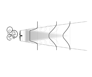
  $x_0$ is usually assumed to be one rotor diameter based on experimental observation (Krogstad & Adaramola Reference Krogstad and Adaramola2012) and one-dimensional momentum theory (Hansen Reference Hansen2015) for a turbine operating in the optimal tip speed ratio. This assumption is consistent with the concept of expansion region proposed by Crespo et al. (Reference Crespo, Hernandez and Frandsen1999). In the expansion region, the pressure builds up to reach the ambient pressure, and the shear layer growth is negligible compared with the rotor diameter. Figure 3 presents a schematic of the mixing layer growth, and the wake velocity profile transformation from a top-hat shape in the near wake to a self-similar Gaussian profile in the far wake. At each downstream location, an estimation of the wake centreline velocity is required. In the self-similar region of the wake, this value is calculated from the Gaussian wake model derived based on mass and momentum conservation (Bastankhah & Porté-Agel Reference Bastankhah and Porté-Agel2014):
 \begin{equation} \frac{U_{{centre}}(x)}{U_{\infty}} = \sqrt{1 - \frac{C_T}{8(\sigma_{{wake}}(x)/d)^2}} . \end{equation}
In the near-wake region, with the help of one-dimensional momentum theory (Hansen Reference Hansen2015), it can be shown that the normalised wake centreline velocity should not fall below  $\sqrt {1 - C_T}$. As in this region the wake does not reach the full self-similar Gaussian shape, (2.16) is not valid and either diverges or yields values less than $\sqrt {1 - C_T}$. Therefore, the normalised wake centreline velocity is set to $\sqrt {1 - C_T}$ in the near-wake region (Abkar, Sørensen & Porté-Agel Reference Abkar, Sørensen and Porté-Agel2018).

Figure 3. Schematic of the gradual growth of the mixing layer from the wake edge and the wake velocity distribution from the near wake (top-hat) to the far wake (self-similar Gaussian).
As at each downstream location the centreline velocity is not known prior to the mixing layer characteristic length, one should deploy an iterative method between (2.15) (including the travel time calculation (2.14) and filtering) and (2.16). Technically, at each downstream location, the  $U_{{centre}}$ is initialised with the previous location value to have an initial estimation of the advection velocity, travel time and filtered velocity to solve (2.15). The estimated length scale is then used to update the centreline velocity. This iterative procedure is repeated until convergence. As the velocity deficit in the wake has a smooth decreasing form, the computational cost of the iterative process is insignificant. A key step of the new framework is the estimation of $\sigma _{{wake}}$ (Gaussian wake width) based on the mixing layer characteristic length ( $\sigma _e$). For this purpose, we profit from the presented analogy between wind turbine wake expansion and scalar diffusion from a continuous disk source in § 2.1.3 to correlate the mixing layer characteristic length ( $\sigma _{e}$) and the Gaussian profile standard deviation ( $\sigma _{{wake}}$) at each downstream location. Therefore, by using this relation (equation (2.8)) the model is closed.
All the aforementioned derivations were based on the lateral velocity component. However, there is no limitation to extend the methodology to the vertical direction by replacing  $\langle {v}_{(T/\beta )}^2 \rangle ^{{1}/{2}}$ with $\langle w_{(T/\beta )}^2 \rangle ^{{1}/{2}}$. Several numerical and experimental studies have shown that despite the differences between $\langle {v}^2 \rangle$ and $\langle w^2 \rangle$ in the ABL, wind turbines wakes are fairly axisymmetric and they can be represented by an equivalent wake width that can be defined as the geometrical mean of wake widths in the spanwise and vertical directions ( $\sigma _{{wake,tot}} = \sqrt {\sigma _{{wake,y}} \sigma _{{wake,z}}}$) (Abkar & Porté-Agel Reference Abkar and Porté-Agel2015; Xie & Archer Reference Xie and Archer2015; Cheng & Porté-Agel Reference Cheng and Porté-Agel2018).
In summary, in order to calculate the wake width at each downwind location, one should solve (2.15), along with the travel time (2.14) and centreline velocity (2.16) while using (2.8) to correlate the mixing layer characteristic length to the wake width. The primary input for the new wake model is a velocity time series sampled upstream of the turbine at hub height. Within the framework of the current study, this signal is sampled from LESs of a fully developed turbulent flow under neutral atmospheric conditions.
2.3. Near-wake length
In this section, we derive a new relation for the near-wake length based on the incoming atmospheric turbulence and turbine operating conditions. For the model presented in § 2.2, one should calculate the near-wake length before solving (2.15). As mentioned earlier, in the near-wake region, one can assume that the centreline velocity is constant ( $U_{{centre}} = U_{\infty }\sqrt {1 - C_T}$). By this assumption, the advection and shear velocity can be simplified as a function of the free-stream velocity and turbine operating condition:
 \begin{equation} \left.\begin{matrix} U_{{adv}} = 0.5(U_{\infty} + U_{{centre}}) = 0.5 U_{\infty}(1 + \sqrt{1 - C_T}) , \\ {\rm \Delta} U_{{max}} = U_{\infty} - U_{{centre}} = U_{\infty}(1 - \sqrt{1 - C_T}) . \end{matrix}\right\} \end{equation}
Moreover, to include the lateral and vertical velocity components contribution to the near-wake length, based on the axisymmetric growth of the turbine wakes, one possible approach is to introduce the equivalent filtered velocity as the geometrical mean of the lateral and vertical components. By applying these assumptions to (2.13), the spreading equation can be written as follows:
 \begin{equation} \sigma_{e,NW} = \frac{1}{U_{{adv}}}(\sqrt{Sc_t} \sqrt{\langle {v}_{(T/\beta)}^2 \rangle^{{1}/{2}} \langle w_{(T/\beta)}^2 \rangle^{{1}/{2}}} + S'{\rm \Delta} U_{{max}})(x_{NW} - x_{0}) , \end{equation}
where  $x_{NW}$ is the length of the near wake, $\sigma _{e,NW}$ is the mixing layer characteristic length at the end of the near wake, and $x_{0}$ represents the expansion region length ( $\approx 1d$). By solving (2.18) for $x_{NW}$, the following relation is obtained for the near-wake length:
 \begin{equation} \frac{x_{NW}}{d} = \frac{\sigma_{e, NW}}{d} \frac{U_{\infty}(1 + \sqrt{1 - C_T})}{2(\sqrt{Sc_t}\sqrt{\langle {v}_{(T/\beta)}^2 \rangle^{{1}/{2}} \langle w_{(T/\beta)}^2 \rangle^{{1}/{2}}} + U_{\infty}S'(1 - \sqrt{1 - C_T}))}+\frac{x_{0}}{d} . \end{equation}
This equation provides an estimation of the near-wake length based on the incoming ambient turbulence and turbine operating conditions. By including the filtered velocity components, one ensures that the relevant scales of the incoming turbulence are contributing to the wake growth rate until the end of the near wake. Since the corresponding travel time is not known prior to the near-wake length, an iterative method should be used to solve (2.19). In order to avoid the iterative method of (2.19) for the near-wake length calculation, one can introduce the following simplifications for (2.19) to provide simpler forms to estimate the near-wake length based on the following assumptions.
• As the near-wake region is relatively close to the turbine and the travel time is small, one can assume that all the turbulence scales contribute to the wake expansion in that region. By this assumption, one can approximate $\langle {v}_{(T/\beta )}^2 \rangle ^{{1}/{2}}$ ($\langle w_{(T/\beta )}^2 \rangle ^{{1}/{2}}$) as $I_v U_{\infty }$ ($I_w U_{\infty }$) where $I_v$ ($I_w$) is the lateral (vertical) turbulence intensity. Therefore, (2.19) can be rewritten as
(2.20)\begin{equation} \frac{x_{NW}}{d} = \frac{\sigma_{e, NW}}{d} \frac{1 + \sqrt{1 - C_T}}{2( \sqrt{Sc_t}(\sqrt{I_vI_w}) + S'(1 - \sqrt{1 - C_T}))} +\frac{x_{0}}{d} . \end{equation}
$\langle {v}_{(T/\beta )}^2 \rangle ^{{1}/{2}}$ ($\langle w_{(T/\beta )}^2 \rangle ^{{1}/{2}}$) as $I_v U_{\infty }$ ($I_w U_{\infty }$) where $I_v$ ($I_w$) is the lateral (vertical) turbulence intensity. Therefore, (2.19) can be rewritten as
(2.20)\begin{equation} \frac{x_{NW}}{d} = \frac{\sigma_{e, NW}}{d} \frac{1 + \sqrt{1 - C_T}}{2( \sqrt{Sc_t}(\sqrt{I_vI_w}) + S'(1 - \sqrt{1 - C_T}))} +\frac{x_{0}}{d} . \end{equation}• For the particular case of near-neutral atmospheric conditions, the standard deviation of the three velocity components can be scaled with the friction velocity (
$\sigma _u \approx 2.5u_*, \sigma _v \approx 1.9u_*,\sigma _w \approx 1.3u_*$) in the surface layer (Panofsky Reference Panofsky1984). These scalings are only valid in the neutral surface layer. Therefore, under neutral conditions, we can further simplify (2.20) as follows:
(2.21)\begin{equation} \frac{x_{NW}}{d} = \frac{\sigma_{e, NW}}{d} \frac{1 + \sqrt{1 - C_T}}{2( \sqrt{Sc_t}(0.63 I_u) + S'(1 - \sqrt{1 - C_T}))} +\frac{x_{0}}{d} . \end{equation}


In order to estimate the near-wake length with (2.19)–(2.21), the value of  $\sigma _{e,NW}/d$ should be specified. As shown in figure 2(a) and discussed in § 2.1.3, the $R^2$ reaches to $0.99$ for $\sigma _{e}/d \approx 0.18$. The $R^2 = 0.99$ criterion is often used as a threshold to determine the onset of the self-similar Gaussian behaviour of the far wake in experimental (Carbajo Fuertes et al. Reference Carbajo Fuertes, Markfort and Porté-Agel2018) and numerical studies (Sørensen et al. Reference Sørensen, Mikkelsen, Henningson, Ivanell, Sarmast and Andersen2015). Therefore, by using $\sigma _{e,NW}/d \approx 0.18$, (2.19)–(2.21) are closed relations.
2.4. Simplified form of spreading equation
In this section, we aim to find a simplified form of the filtering operator in (2.15) and present a computationally faster implementation for the wake width calculation with a reasonable accuracy. As stated by (2.1), the original form of Taylor diffusion theory is based on the velocity ACF. As a well-known approximation (Taylor Reference Taylor1922; Neumann Reference Neumann1978; Hanna et al. Reference Hanna, Briggs and Hosker1982), ACF can be written in a simple exponential form:
 \begin{equation} R(T) = \exp \left(-\frac{T}{T_{L}}\right) , \end{equation}
in which  $T$ is the travel time from the source and $T_{L}$ is the Lagrangian integral time scale. By replacing (2.22) in (2.1), performing the integration for the lateral velocity component, and introducing the Lagrangian integral time scale for the lateral velocity time series as $T_{Lv}$, the following form for the particle distribution behind a source is derived:
 \begin{equation} \sigma_y ^2 (T) = 2\sigma_v^2T T_{Lv} - 2\sigma_v^2T_{Lv}^2 \left(1 - \exp \left(\frac{-T}{T_{Lv}}\right)\right) . \end{equation}
From a practical point of view, fixed-point measurements are more feasible than particle tracking methods to estimate the diffusion properties. Therefore, to calculate the Lagrangian integral time scale, one can estimate the integral time scale from a fixed point time series measurement (based on the definition used by Hanna (Reference Hanna1981), the integral time scale is equal to the time lag where the ACF first drops to  $1/e$) and then use the previously defined scale factor $\beta$. Following the derivation presented in Pasquill & Smith (Reference Pasquill and Smith1983), one can write the particle distribution as a function of the travel time and filtered velocity:
 \begin{equation} \sigma_y ^2 (T) = \langle {v}_{(T/\beta)}^2 \rangle T^2 . \end{equation}
By equating (2.23) and (2.24), the lateral filtered velocity for each travel time can be written as follows:
 \begin{equation} \langle {v}_{(T/\beta)}^2 \rangle^{{1}/{2}} = \frac{\sigma_v T_{Lv}}{T}\sqrt{2 \left( \frac{T}{T_{Lv}} - \left(1 - \exp \left(\frac{-T}{T_{Lv}}\right)\right) \right )} , \end{equation}
where  $\sigma _v$ is the standard deviation of the lateral velocity component. Therefore, the simplified version of spreading (2.15) for the lateral mixing layer characteristic length ( $\sigma _{ey}$) can be written as follows:
 \begin{equation} \sigma_{ey}(x) = \underbrace{T \sqrt{Sc_t} \frac{\sigma_v T_{Lv}}{T} \sqrt{2\left(\frac{T}{T_{Lv}} - (1 - \exp (\frac{-T}{T_{Lv}})) \right ) }}_\text{{Ambient flow}} + \underbrace{2S'(U_{\infty}T - (x-x_0))}_\text{{Turbine-induced}} . \end{equation}
One can simplify the travel time in the ambient flow term to have a more compact form:
 \begin{equation} \sigma_{ey}(x) = \underbrace{ \sqrt{Sc_t} \sigma_v T_{Lv}\sqrt{2\left( \frac{T}{T_{Lv}} - \left(1 - \exp \left(\frac{-T}{T_{Lv}}\right)\right) \right ) }}_\text{{Ambient flow}} + \underbrace{2S'(U_{\infty}T - (x-x_0))}_\text{{Turbine-induced}} . \end{equation}
Equation (2.27) can be used instead of (2.15) to calculate the lateral mixing layer characteristic length with a simpler method that does not require explicit filtering of the velocity time series by an external function. The range of validity of (2.27) is the same as that of the model presented in § 2.2; one can solve (2.27) from the end of the expansion region ( $x_0$) until the desired downwind distance. At each downstream location, the travel time is calculated from (2.14), the centreline velocity is either constant (near wake) or calculated from the Gaussian wake model (far wake), and the mixing layer characteristic length and the Gaussian wake width are correlated through (2.8). As in the model presented in § 2.2, there is no limitation to extend (2.27) to the vertical direction with the respective properties. This equation can be solved easily without any external function for filtering the velocity time series, and predicts the wake width in a fast and easy to implement manner.
2.5. Near-wake treatment: a new form for the velocity deficit distribution
This section focuses on introducing a new formulation for the super-Gaussian shape function to predict the wake velocity deficit distribution in the near wake. By definition, the super-Gaussian shape function allows the transition from a top-hat distribution to a Gaussian profile with a single functional form. Based on the presented analogy of wind turbine wake expansion and scalar diffusion from a disk source, the goal is to propose a new method to determine the super-Gaussian shape function parameters for the near-wake velocity deficit distribution that asymptotes to the Gaussian wake model in the far wake. It should be noted that the derivation presented in the following closely follows the steps proposed by Blondel & Cathelain (Reference Blondel and Cathelain2020). We start by assuming that the non-dimensional wake velocity deficit has a super-Gaussian form:
 \begin{equation} \frac{\Delta U(x)}{U_{\infty}} = C^{\prime}(x)f(x,r) = C^{\prime}(x) \exp \left(-\frac{r^{n(x)}}{2\sigma^{'2}(x)}\right) , \end{equation}
where  $C^{\prime }(x)$ is the wake maximum velocity deficit, $f(x,r)$ is the shape function, $r$ is the radial distance from the wake centre, $n(x)$ is the smoothness parameter and $\sigma ^{\prime }(x)$ is the super-Gaussian wake width (when $n =2$, $\sigma ^{\prime }(x)$ is the wake standard deviation). By neglecting the viscous and pressure terms in the momentum equation, the following integral can be derived for conserving mass and momentum (Tennekes & Lumley Reference Tennekes and Lumley1972):
 \begin{equation} 2{\rm \pi} \rho \int_{0}^{\infty} U_{w}(U_{\infty} - U_{w})r\, {\rm d} r = T , \end{equation}
where  $\rho$ is the air density and $T$ is the turbine thrust force. By replacing (2.28) in (2.29) and integrating, the following relation between the maximum velocity deficit, super-Gaussian wake width, smoothness parameter and turbine thrust coefficient is derived including the Gamma function ( $\varGamma$):
 \begin{equation} C^{'2}(x) - 2^{2/n(x)} C^{\prime}(x) + \frac{n(x)C_T}{16 \varGamma(2/n(x))\sigma^{'4/n(x)}} = 0 . \end{equation}
 Within the framework of the presented analytical model (§ 2.2), the maximum velocity deficit is known after solving the model at each downstream location. However, the smoothness parameter and the super-Gaussian wake width are not known. In order to define a super-Gaussian shape function that predicts the velocity deficit distribution in the near wake and converges to a self-similar Gaussian profile in the far wake, we propose a new expression for the smoothness parameter. The choice of the smoothness parameter is made to guarantee that the super-Gaussian prediction smoothly transitions to a self-similar Gaussian distribution in the far wake ( $n(x) = 2$), which is consistent with the aforementioned Gaussian model results in that region. In addition, one should consider that the near-to-far-wake transition occurs at different downwind locations based on the incoming flow turbulence level. In order to fulfil the conditions listed above, we propose the following form for the smoothness parameter variation in the wind turbine wake:
 \begin{equation} n(x) = 2 + A \,\mathrm{erfc}\left(\frac{2 (\sigma_{e}(x)/d)}{0.18}\right) , \end{equation}
where  $\sigma _{e} (x)/d$ is the total mixing layer characteristic length (geometrical mean of the lateral and vertical characteristic lengths) at each downwind location, $0.18$ corresponds to the near-wake criterion introduced in § 2.3 and $A$ is a tunable parameter which defines the smoothness of the super-Gaussian profile at the end of expansion region ( $n(x_0) = 2 + A$). This form ensures that the smoothness parameter converges to two in the far wake and the super-Gaussian shape function switches to the Gaussian wake model. At this point, with the smoothness and maximum velocity deficit known at each downstream location, one can solve (2.30) for the super-Gaussian wake width:
 \begin{equation} \sigma^{\prime}(x) = \left( \frac{n(x)C_T}{2^{2/n(x)}C^{\prime}(x) - C^{'2}(x)} \frac{1}{16 \varGamma(2/n(x))} \right)^{(n(x)/4)} . \end{equation}
Therefore, by calculating the super-Gaussian wake width at each downstream location, the super-Gaussian shape function is fully defined and can provide the wake velocity deficit distribution in the near wake and provides the correct asymptotic behaviour in the far wake.
3. Model validation
3.1. LES framework
To validate the model and test its performance, a series of LESs of a utility-scale wind turbine wake under neutral ABL conditions were performed with the in-house LES code developed at the WiRE Laboratory of EPFL (WiRE-LES). The code solves the filtered incompressible Navier–Stokes equation:
 \begin{gather} \frac{\partial \tilde{u}_i}{\partial x_i} = 0 , \end{gather}
 \begin{gather}\frac{\partial \tilde{u}_i}{\partial t} + \tilde{u}_j \frac{\partial \tilde{u}_i}{\partial x_j} ={-} \frac{\partial \tilde{p}^*}{\partial x_i} - \frac{\partial \tau_{ij}}{\partial x_j} - f_i , \end{gather}
where  $i = 1, 2, 3$ refers to the streamwise, spanwise and vertical directions, respectively, $\tilde {u}$ is the filtered velocity, $\tilde {p}^*$ is the filtered modified kinematic pressure, $\tau$ is the kinematic sub-grid scale (SGS) stress and $f$ represents the additional effects such as an external forcing to drive the flow or the turbine forces. The code is based on pseudo-spectral schemes in the horizontal directions and second-order centred finite-difference scheme in the vertical direction. The horizontal boundary conditions are periodic, a flux-free boundary condition is used at the top, and the bottom boundary condition is set through the local application of the Monin–Obukhov similarity theory. For time advancement, the second-order Adams–Bashforth explicit scheme is used. Within the WiRE-LES framework, the Lagrangian scale-dependent dynamic model (Stoll & Porté-Agel Reference Stoll and Porté-Agel2006) is used to parametrise the SGS turbulent fluxes and the rotational actuator disk model is used to model the turbine-induced forces (Wu & Porté-Agel Reference Wu and Porté-Agel2011). The WiRE-LES has been validated in several studies of ABL flows with the presence of wind turbines (Porté-Agel et al. Reference Porté-Agel, Wu, Lu and Conzemius2011; Wu & Porté-Agel Reference Wu and Porté-Agel2011; Porté-Agel, Wu & Chen Reference Porté-Agel, Wu and Chen2013; Revaz & Porté-Agel Reference Revaz and Porté-Agel2021).
In this study, a domain size of  $L_x = 3840\ \mathrm {m}$, $L_y = 1920\ \mathrm {m}$, $L_z = 955\ \mathrm {m}$ is uniformly divided into $N_x = 256$, $N_y = 192$, $N_z = 192$ grid points. The simulations, as listed in table 1, cover a wide range of incoming turbulence levels and are driven by a constant streamwise pressure gradient up to $0.8L_z$ to maintain a hub height velocity of 8 m s $^{-1}$. To minimise the effect of the top boundary on the flow, no forcing is applied in the top 20 % of the domain. The inflow is generated through a set of precursor simulations and imposed on the simulations with the turbine. The wind turbine has a diameter of 80 m and a hub height of 70 m and is placed 12 rotor diameters after the inlet. In this condition, the turbine has an almost constant thrust coefficient of 0.8. To avoid numerical instabilities, the parametrised turbine forces are distributed smoothly on the computational grid with the help of a Gaussian kernel (Mikkelsen Reference Mikkelsen2003). To guarantee mesh independent results, the grid spacing is chosen to cover the rotor diameter with 8 points in the spanwise direction and 16 points in the vertical direction. These values satisfy the minimum grid points required in the spanwise direction (at least five cells) and vertical direction (at least seven cells) across the rotor diameter (Wu & Porté-Agel Reference Wu and Porté-Agel2011, Reference Wu and Porté-Agel2012).
Table 1. Incoming turbulence intensity of LES cases at turbine hub height:  $I_u$, $I_v$ and $I_w$ denote the streamwise, spanwise and vertical turbulence intensities, respectively, and $z_0$ corresponds to the surface roughness.

3.2. Results and discussion
In this section, we assess the performance of two forms of the new analytical model (hereafter, ‘Model Filter’ is used to denote the form presented in § 2.2, whereas the simplified form presented in § 2.4 is denoted as ‘Model ITS’ in which ITS stands for integral time scale) by comparing its predictions against results from LESs of the wake of a utility scale wind turbine. Several cases are considered, corresponding to a wide range of turbulence intensities in the incoming flow under neutral atmospheric conditions, as summarised in table 1. For all the LES cases, the simulated wake velocity deficit distribution is fitted with a Gaussian profile in the lateral direction and a Gaussian profile with ground reflection in the vertical direction. As discussed earlier, wind turbine wakes are fairly axisymmetric with similar growth rates in the lateral and vertical directions (Cheng & Porté-Agel Reference Cheng and Porté-Agel2018). Therefore, the geometrical mean of the lateral and vertical wake widths is considered as the total wake width ( $\sigma _{{wake,tot}} = \sqrt {\sigma _{{wake,y}} \sigma _{{wake,z}}}$). In order to compare the LES results with the predictions from the new analytical model, the latter uses as input the incoming flow information from a velocity time series sampled during the LES simulations, upstream of the turbine at hub level. Using the incoming flow information, the model computes the total wake width at each downwind distance. It should be mentioned that Model Filter and Model ITS can estimate the total wake width from 1d to the desired downwind distance. For this study and the mentioned cases, both models are used in the range of 1d to 20d. Regarding the model parameters, $Sc_t = 0.5$ (Reynolds Reference Reynolds1976), $S' = 0.043$ (§ 2.1.2), $x_0/d = 1$ (§ 2.2) and $\sigma _{e,NW}/d = 0.18$ (§ 2.1.3), are used based on the presented discussions in § 2, without any parameter tuning.
Figure 4 shows a comparison of the wake width as a function of the downwind distance computed from the new analytical model, the empirical wake growth rate relations proposed by Niayifar & Porté-Agel (Reference Niayifar and Porté-Agel2016) and Teng & Markfort (Reference Teng and Markfort2020), and that obtained from the LES data. As shown in this figure, the proposed model can predict the wake width reasonably well within a wide range of incoming turbulence levels. In comparison with the empirical relations of the wake growth rate (with different tuned parameters), the model shows a reasonable prediction across a wide range of turbulence levels. As can be noted from figure 4, the wake growth rate relation proposed by Niayifar & Porté-Agel (Reference Niayifar and Porté-Agel2016) provides reasonable wake width predictions in comparison with the LES data, whereas the relation proposed by Teng & Markfort (Reference Teng and Markfort2020) underestimates the wake width in the presence of low turbulence intensity in the incoming flow. The new physics-based model captures the start of the wake expansion at the beginning of the far wake, followed by an approximately linear growth rate with the downwind distance. At farther downstream distances (greater than around 12d, depending on the atmospheric turbulence level), the wake expansion rate gradually decreases from the initial linear growth rate. This is due to the fact that, by increasing downstream distance, the range of effective ambient turbulence scales contributing to the wake expansion (i.e. turbulent eddies of size equal or larger than the wake width) decreases. The proposed model can capture that effect and the associated nonlinear wake expansion rate, which is crucial for the prediction of wind farm wakes using analytical wake models. Moreover, figure 4 highlights the importance of including the effect of turbine-induced turbulence on the turbulent viscosity. By including this term, the model provides an acceptable prediction and avoids the underestimation of the wake growth rate associated with the use of only atmospheric turbulence in the definition of the turbulence viscosity (Cheng & Porté-Agel Reference Cheng and Porté-Agel2018).

Figure 4. Normalised total wake width as a function of streamwise distance. The circles indicate LES results, the solid lines are the solution obtained from Model Filter as presented in § 2.2 and the dashed lines are the solution from the simplified approach, Model ITS in § 2.4. The prediction by the empirical wake growth rate relations proposed by Niayifar & Porté-Agel (Reference Niayifar and Porté-Agel2016) and Teng & Markfort (Reference Teng and Markfort2020) are also shown.
Figure 5 shows the change of the maximum normalised velocity deficit, at the turbine hub height, as a function of downwind distance computed from the new analytical model, the Gaussian wake model with the empirical wake growth rate relations proposed by Niayifar & Porté-Agel (Reference Niayifar and Porté-Agel2016) and Teng & Markfort (Reference Teng and Markfort2020), and that obtained from LES data. As shown in this figure, the model can predict the maximum wake velocity deficit in a wide range of incoming turbulence levels reasonably well. Note that the assumption of the expansion region downstream of the turbine and the uniform velocity distribution in the near-wake region is consistent with the LES results. The maximum velocity deficit has an approximately uniform distribution in the near wake and decreases gradually after the near-to-far-wake transition point (shown in figure 5 as ‘Near-wake LES’). The comparison between the LES data and the wake velocity deficit predicted by the Gaussian model using the empirical relations for the wake growth rate shows the sensitivity of the predictions to the empirical constant. The Gaussian wake model with the proposed relation by Niayifar & Porté-Agel (Reference Niayifar and Porté-Agel2016) can provide reasonable predictions for the wake velocity deficit, whereas using the relation by Teng & Markfort (Reference Teng and Markfort2020) overestimates the wake velocity deficit in the presence of low turbulence intensity in the incoming flow. In addition, figure 5 shows a comparison between the near-wake length of the LES cases and the near-wake length of the model, which is discussed in more detail later in this section. As can be noted in figures 4 and 5, Model Filter and Model ITS can predict the wake growth rate and the maximum wake velocity deficit downstream of the turbine reasonably well. There exist slight differences between the two methods due to the different approaches to compute the standard deviation of the filtered velocity. Based on the presented results, one can conclude that the proposed model can provide fast and reasonably accurate predictions of the wake width under a wide range of incoming turbulence conditions.

Figure 5. Normalised maximum velocity deficit as a function of streamwise distance. The vertical dotted line corresponds to the near-wake length from LES cases and the vertical dash-dotted line corresponds to the near-wake length obtained from (2.19). For the legend refer to the caption of figure 4.
Figure 6 shows a comparison of the lateral profiles of the normalised velocity deficit downwind of the turbine at hub level calculated by the proposed model, the Gaussian wake model with the empirical wake growth rate relations proposed by Niayifar & Porté-Agel (Reference Niayifar and Porté-Agel2016) and Teng & Markfort (Reference Teng and Markfort2020), and those obtained from the simulations. It should be noted that the new analytical model, as presented in § 2.2, uses the Gaussian wake model to calculate the wake velocity deficit profiles in the far wake (figure 6,  $x/d = 6, 10, 15$). In the near wake (figure 6, $x/d = 2$), the wake velocity deficit profiles are calculated using the new super-Gaussian form as presented in § 2.5. The proposed framework allows the calculation of the wake velocity deficit profiles in the near wake with the super-Gaussian form consistent with the Gaussian wake model by ensuring the super-Gaussian smoothness parameter ( $n$) is equal to two in the far-wake region. For the reported results, the value of the super-Gaussian model parameter ( $A$) is set to 12. It is worth mentioning that the optimum value of $A$ could depend on the turbine operating condition ( $C_T$) and it is not universal. As shown in the figure, in the near wake, the new super-Gaussian form predicts the wake velocity deficit distribution reasonably well (figure 6, $x/d = 2$). These detailed comparisons within a wide range of incoming turbulence conditions, as shown in figures 4, 5 and 6, validate the new analytical model.

Figure 6. Normalised velocity deficit profiles at different streamwise locations for all the cases.
As discussed in § 2.2, the wake advection velocity at each downwind location is not known prior to the wake width and wake centreline velocity, and one should deploy an iterative scheme to calculate these quantities at each downstream location. In addition to the definition of wake advection velocity presented in this study, other approaches have been used to estimate this quantity. For example, in the dynamic wake meandering model (Larsen et al. Reference Larsen, Madsen, Thomsen and Larsen2008), the wake advection velocity is assumed to be equal to the free stream velocity ( $U_{{adv}} = U_{\infty }$). In order to explore how different values of the wake advection velocity affect the new analytical model outputs, we compare the model results, as presented in § 2.2, for four different approaches to calculate the advection velocity: (1) $U_{{adv}}(x) = 0.5(U_{\infty } + U_{{centre}}(x))$, (2) $U_{{adv}}(x) = U_{\infty }$, (3) $U_{{adv}}(x) = 0.5U_{\infty }(1 + \sqrt {1-C_T}) \xrightarrow []{\text C_T = 0.8} U_{{adv}}(x) = 0.72U_{\infty }$ and (4) $U_{{adv}}(x) = 0.5(0.72U_{\infty } + U_{\infty })= 0.86U_{\infty }$. These approaches cover the original formulation of the advection velocity in the new model (approach 1), the constant advection velocity proposed by the dynamic wake meandering model (approach 2) and the constant advection velocity equal to the average of the free stream and theoretical near-wake centreline velocity from one-dimensional momentum theory (approach 3). For the last approach, the advection velocity is defined as the average of approaches 2 and 3, allowing us to analyse the model outputs in the middle of these two limits. Figure 7 shows the change of the maximum normalised velocity deficit, at the turbine hub level, as a function of normalised downwind distance for the proposed approaches and that obtained from LES data. As can be noted, all the approaches provide similar asymptotic behaviour in the very far wake at downstream distances greater than 12d. For shorter distance from the turbine, the assumption of $U_{{adv}} = U_{\infty }$ provides an overly fast advection of the wake that results in a shorter travel time for a fixed downwind distance compared with the LES results. As a result, and as shown in figure 7, this assumption causes an overly slow wake recovery and a clear overestimation of the wake velocity deficit in the far wake up to downstream distances of about six to eight rotor diameters (depending on the atmospheric turbulence level) in comparison with the LES results. On the other hand, the assumptions of $U_{{adv}} =0.72 U_{\infty }$ and $U_{{adv}} =0.86 U_{\infty }$ provide predictions of the maximum wake velocity deficit that are closer to those obtained with LES simulations. This can be explained by the fact that, for those distances, these values are closer to the expected advection velocity reported in the literature and defined in § 2.2. Therefore, the approach for estimating the advection velocity can influence the wake velocity deficit prediction, particularly in the far wake up to downwind distances of about six to eight rotor diameters.

Figure 7. Normalised maximum velocity deficit as a function of streamwise distance in the far wake, comparison of four different approaches to calculate the advection velocity.
Next, we use the model to analyse the contribution of each term to the wake width in more detail. Figure 8 shows the average contribution of the ambient and the turbine-induced turbulence to the total wake width calculated with the new model as a function of radial turbulence intensity ( $\sqrt {I_vI_w}$). The relative contribution of each term in the model for the presented cases in table 1 and the theoretical limits in the extreme of no ambient turbulence are shown in the figure with the symbols. One can observe a considerable increase in the relative contribution of the turbine-induced turbulence by decreasing the turbulence intensity of the incoming ABL flow. In the case with the lowest ambient turbulence (with streamwise turbulence intensity of $0.05$), the turbine-induced turbulence contribution to the wake width is around $40\,\%$ of the total wake width. To further investigate the relative contribution of the ambient and turbine-induced turbulence to the wake width under a wide range of ambient radial turbulence intensities (from 0 to 0.1), we have used the Model ITS as presented in § 2.4. In that model, the Eulerian integral scale was chosen as the average of those calculated from the five LES cases, as it was found to have a relatively small variability (standard deviation to mean ratio smaller than 0.15). The results are also shown in figure 8 as a dash-dotted line (ambient-turbulence contribution) and a dashed line (turbine-induced contribution). The relative contribution of each term shows a steeper variation with decreasing ambient turbulence intensity. This trend emphasises the importance of the turbine-induced turbulence term of the model for the accurate prediction of the wake growth rate in relatively low ambient turbulence conditions. Further research is required to fill the gap in this region of interest and explore the behaviour of the contributing factors to the wake expansion in the extreme of low turbulence. The importance of the turbine-induced turbulence, along with the limitations of the current empirical formulations for the wake growth rate parameter (a function of the streamwise turbulence intensity alone and valid within a limited range of turbulence intensity levels) supports the importance of having a physics-based model that considers both the effects of ambient turbulence and turbine-induced turbulence.

Figure 8. Relative contribution of the ambient (circle) and turbine-induced (square) turbulence to the total wake width computed with the new model as a function of radial turbulence intensity. The theoretical limits in the extreme of no ambient turbulence are also shown in the figure. The dashed (turbine-induced) and dash-dotted (ambient) lines show the variation of each term as a function of radial turbulence intensity obtained from Model ITS (§ 2.4).
Figure 9 shows the variation of the near-wake length with the streamwise turbulence intensity calculated from the proposed relations (2.19)–(2.21), and it is compared with that obtained from the near-wake length model proposed by Bastankhah & Porté-Agel (Reference Bastankhah and Porté-Agel2016), the near-wake length model proposed by Vermeulen (Reference Vermeulen1980) and LES data. For the LES data, the near-wake length is calculated based on the downstream position where the linear correlation coefficient of the Gaussian fit to the velocity deficit reaches the threshold of  $0.99$. For the proposed relations in § 2.3, the value of the parameters are the same as those mentioned earlier ( $Sc_t = 0.5$, $S' = 0.043$, $x_0/d = 1$, $\sigma _e/d = 0.18$) without any parameter tuning. The other models are used with their original set of parameters. As shown in this figure, the near-wake length increases with decreasing ambient turbulence level. Equations (2.19)–(2.21) capture this behaviour and provide an acceptable prediction of the near-wake length in a wide range of ambient turbulence levels. It should be mentioned that (2.20) is a simplified form of (2.19) based on removing the filtering from the equivalent radial velocity component and (2.21) is strictly valid for neutral atmospheric conditions. Thus, the use of each of the proposed equations should take into account their respective underlying assumptions.

Figure 9. Near-wake length as a function of streamwise turbulence intensity, comparison of the proposed relations (2.19)–(2.21), LES results, the near-wake length proposed by Bastankhah & Porté-Agel (Reference Bastankhah and Porté-Agel2016) and the near-wake length proposed by Vermeulen (Reference Vermeulen1980).
4. Summary and concluding remarks
In this study, a new physics-based model has been proposed to predict the wake growth rate downstream of a wind turbine. The model is based on the Taylor diffusion theory, the Gaussian wake model, turbulent mixing layers self-similarity and the similarity between wind turbine wake expansion and scalar diffusion from a disk source. With these elements in place, the model ensures the conservation of mass and momentum in the far wake and accounts for the effects of both ambient turbulence and turbine-induced turbulence on the total wake width at each downstream location. Moreover, by filtering the velocity time series at each downwind distance, the model takes into account the relevant scales of the incoming turbulence in the wake expansion and removes the high-frequency fluctuations (small scales). A simplified version of the model has also been derived and only requires as inputs the unfiltered velocity standard deviation and the integral time scales of the radial velocity component of the incoming flow. Another outcome of the proposed modelling framework is a new relation for the near-wake length as a function of the incoming ambient turbulence intensity and turbine operating condition ( $C_T$). In addition, a new functional form for the wake velocity deficit distribution in the near wake has been derived based on a super-Gaussian shape function and a new approach to calculate the smoothness parameter.
The model performance has been validated against LES data of a utility-scale wind turbine wake under neutral ABL conditions with a wide range of incoming ambient turbulence levels. It has been found that the proposed model yields reasonably accurate predictions of the wake width, normalised maximum velocity deficit and near-wake length for all the LES cases. It is particularly noteworthy to mention that the model performs well for low ambient turbulence conditions, for which the existing models are unable to account for the contribution of turbine-induced turbulence on the wake expansion. In summary, the proposed analytical model is found to be simple, fast and reasonably accurate for the prediction of mean turbine wake flows under a wide range of atmospheric turbulence conditions.
Future research will focus on extending the proposed analytical model to calculate the wake velocity deficit distribution inside wind farms with different layout configurations. Moreover, the analytical modelling framework presented in this study should be further tested and, if needed, improved to capture the effect of thermal stability on wind turbine wakes.
Acknowledgements
Computing resources were provided by EPFL through the use of the facilities of its Scientific IT and Application Support Center (SCITAS) and by the Swiss National Super-computing Centre (CSCS).
Funding
This research was funded by the Swiss National Science Foundation (Grant Number 200021_172538) and the Swiss Federal Office of Energy (Grant Number SI/502135-01).
Declaration of interests
The authors report no conflict of interest.
Author contributions
Conceptualisation, D.V. and F.P.-A.; data curation, D.V.; formal analysis, D.V.; funding acquisition, F.P.-A.; investigation, D.V. and F.P.-A.; methodology, D.V. and F.P.-A.; project administration, F.P.-A.; resources, F.P.-A.; software, D.V.; supervision, F.P.-A.; validation, D.V.; visualisation, D.V.; writing–original draft, D.V.; writing–review and editing, D.V. and F.P.-A. Both authors have read and agreed to the published version of the manuscript.
Appendix A. Summary of the model
This section provides a concise summary of the model to facilitate its application by the reader. For this purpose, we review the model inputs, the model outputs and the procedure to calculate the outputs of the model, as well as the key variables.
A.1. Inputs of the model
The inputs to the model are as follows.
(1) Wind turbine thrust coefficient (
$C_T$).(2) For the model presented in § 2.2 (Model Filter), the velocity time series sampled upstream of the turbine at hub height, representing the incoming flow conditions in the streamwise, lateral and vertical directions. For the simplified model presented in § 2.4 (Model ITS), the streamwise, lateral and vertical incoming turbulence intensities and the lateral and vertical integral time scales.
(3) The mean incoming wind speed (
$U_{\infty }$).


The parameters of the model are listed below. The value of each parameter is set based on the presented discussions in § 2, without any parameter tuning.
(1) Turbulent Schmidt number,
$Sc_t = 0.5$ for mixing layers (Reynolds Reference Reynolds1976) (§ 2.2).(2) Mixing layer characteristic length spreading rate,
$S' = 0.043$ (§ 2.1.2).(3) End of the expansion region,
$x_0 = 1d$ (§ 2.2).(4) Threshold for the onset of the far wake,
$\sigma _{e,NW}/d = 0.18$ (§§ 2.1.3 and 2.3).


A.2. Outputs of the model
The outputs of the model are as follows.
(1) Near-wake length (
$x_{NW}$).(2) Wake width (
$\sigma _{{wake}}$).(3) Maximum wake velocity deficit (
$({\rm \Delta} U/U_{\infty })_{{max}}$).(4) Wake velocity deficit distribution.


A.3. Step-by-step procedure
This section provides a summary for the wake analytical model presented in §§ 2.2–2.5 to estimate the near-wake length, the wake expansion, the maximum wake velocity deficit and the wake velocity deficit profiles until the desired downwind distance. The model is proposed in two versions: one based on filtering the velocity time series with a moving average filter (denoted as Model Filter and presented in § 2.2), and a simplified form based on the integral time scales of the incoming flow and the unfiltered velocity standard deviations (denoted as Model ITS and described in § 2.4). The procedure to obtain the model outputs given the inputs mentioned above is as follows.
(1) The near-wake length (
$x_{NW}$) is calculated based on the inflow data using (2.19), or the simplified forms, as presented in (2.20) and (2.21), whenever applicable.(2) For the far wake (
$x \geq x_{NW}$), the Gaussian model given by (2.16) is applied. The wake width and wake centreline velocity are computed using the following streamwise-marching iterative procedure:
(4.1) At each downstream location, the wake centreline velocity (
$U_{{centre}}$) is initialised with the value of the closest upwind position. For each downstream step, from $x_0$ to the position of interest, the travel time ($T$) is computed using (2.14). The wake advection velocity and the shear velocity are computed using the $U_{{centre}}$. For the Model Filter, given the travel time, the respective filter size $(T/\beta )$ can be determined to filter the lateral and vertical velocity time series with the moving average filter.(4.2) The lateral mixing layer characteristic length (
$\sigma _{ey}$) is computed using Model Filter (2.15) or Model ITS (2.27).(4.3) The lateral wake width (
$\sigma _{{wake,y}}$) is computed from $\sigma _{ey}$ using the relation given by (2.8), presented in § 2.1.3.(4.4) Steps (4.2) and (4.3) are repeated for the vertical direction with the respective properties to calculate the
$\sigma _{ez}$ and $\sigma _{{wake,z}}$.(4.5) The total wake width and the total mixing layer characteristic length are calculated as the geometrical mean of the lateral and vertical values.
(4.6) The wake centreline velocity (
$U_{{centre}}$) is computed based on the total wake width using (2.16) in order to guarantee the conservation of momentum.(4.7) The wake advection velocity (
$U_{{adv}}$) is computed, and steps (4.1)–(4.7) are repeated until convergence.
(3) For the near wake (
$x \leq x_{NW}$), the super-Gaussian model given by (2.28), (2.31) and (2.32) is applied. Note that the model is defined in such a way that it smoothly converges to the aforementioned Gaussian solution at the onset of the far wake.


A.4. Key variables
The following is a list of the key variables used in the proposed physics-based analytical modelling procedure.


 Open access