2.1. Definition of the foil kinematic motion

To generate the oscillatory motion of the foil, an active kinematic stroke is applied as

(2.1)\begin{equation} h(t)=-h_{o} \cos(2{\rm \pi} f t),\end{equation}

and

(2.2)\begin{equation} \theta(t)=-\theta_{o} \sin(2{\rm \pi} f t),\end{equation}

where $h(t)$ and $\theta (t)$ are heave and pitch, respectively, with the pitching motion about the midpoint of the chord. The reduced frequency of oscillation, $f$, heave amplitude, $h_o$, and pitch amplitude, $\theta _o$, are the parameters that control the foil motion and are non-dimensionalized by the chord length, $c$, and free-stream velocity, $U_\infty$.

The prescribed sinusoidal heave and pitch of the single foil generates a time-varying effective angle of attack, $\alpha (t)$, with respect to the free-stream flow. A representative effective angle of attack is evaluated when the foil is at maximum heave velocity, which occurs at one quarter of the cycle period, $T$, or

(2.3)\begin{equation} \alpha_{T/4} = \alpha(t=0.25T) = \theta_o - \tan^{-1} \left(\frac{2{\rm \pi} fh_o}{U_{\infty}}\right) , \end{equation}

with $\alpha (t)$ assumed to be in radians and the term $2{\rm \pi} f h_o$ is obtained through the time derivative of the heave motion $\dot {h}(t)$ at $t=0.25T$ (Kim et al. Reference Kim, Strom, Mandre and Breuer2017).

2.2. Computational data utilized in analysis

With the foil kinematic motion defined, the flow over the oscillating foils is simulated at $Re=1000$ using a second-order accurate finite volume, pressure-implicit split-operator algorithm in ${OpenFOAM}$ (Weller et al. Reference Weller, Tabor, Jasak and Fureby1998). The foil shape is a $10\,\%$ thick ellipse, which is convenient for tidal energy due to its fore-aft symmetry. A two-dimensional unstructured dynamic mesh is utilized and the refinement analysis along with the validation of the dynamic mesh against a stationary mesh are presented in Ribeiro et al. (Reference Ribeiro, Su, Guillaumin, Breuer and Franck2021).

Two data sets are considered in this paper. The first set of simulations are a sweep of kinematics of a single oscillating foil with a fully resolved wake (Ribeiro & Franck Reference Ribeiro and Franck2022b). These simulations are used to extract velocity profiles from the wake under various oscillation kinematics, varying the parameters in (2.1) and (2.2).

The second set of simulations have two foils operating in a tandem array configuration at a fixed distance of 6 chords separation. For each array configuration, the inter-foil phase angle, $\psi$, is varied. The kinematic motion for the leading foil (foil 1) is given as

(2.4a,b)\begin{equation} h_1(t)=-h_{o,1} \cos(2{\rm \pi} f t) \quad \theta_1(t)=-\theta_{o,1} \sin(2{\rm \pi} f t),\end{equation}

and for the trailing foil (foil 2),

(2.5a,b)\begin{equation} h_2(t)=-h_{o,2} \cos(2{\rm \pi} f t + \psi) \quad \theta_2(t)=-\theta_{o,2} \sin(2{\rm \pi} f t + \psi),\end{equation}

where the frequency, $f$, remains constant to maintain the same relative phase separation in each stroke. In addition, to reduce the parameter space, the same amplitudes are applied to both foils ($h_{o,1}=h_{o,2}=h_o$; $\theta _{o,1}=\theta _{o,2}=\theta _o$), although this could be varied in future simulations. The inter-foil phase angle ranges from $-180^{\circ }$ to $+180^{\circ }$ with an increment of $30^{\circ }$. The range of foil kinematic parameters investigated in this paper includes $f = 0.10\unicode{x2013}0.15$, $h_o=0.75\unicode{x2013}1.5$ and $\theta _o=55^{\circ }\unicode{x2013}75^{\circ }$ for a total of $16$ sets of kinematics. The parameter range selected is ideal for oscillating foils in energy harvesting mode (Xiao & Zhu Reference Xiao and Zhu2014). For more details on the foil kinematics, see Appendix A.

2.3. Quantifying wake velocity

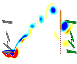
To visualize the parameter space, the schematic in figure 1 displays the foil parameters, the inter-foil spacing, $S_x$, and the swept area, $Y_p$, of a tandem two-foil array where a trailing foil is placed in the leading foil wake. The parameter $Y_p$ is defined as the distance from tip to tip of the foil for a full cycle motion multiplied by the foil span. The wake velocity profile at a streamwise distance $x_w$ downstream from the leading foil is given as

(2.6) \begin{equation} \boldsymbol{u_w}(y,t : x_w) = u(y,t)\hat{\imath} + v(y,t)\hat{\jmath}, \end{equation}

where $u$ and $v$ are the streamwise and cross-flow velocity components, respectively. In this paper the wake velocity extraction is performed at $x_w=5c$, one chord length upstream from the second foil at $x=6c$. The choice of $x_w$ is to provide an accurate representation of the oncoming energy flux in the immediate vicinity of the trailing foil. A recommendation for other configurations (including staggered configurations and in-line of other separation distances) would be to sample the wake at approximately 1 chord upstream of the second foil.

Figure 1. Leading foil (foil 1) parameters and placement of a trailing foil (foil 2) to form a two tandem foil array. Vorticity flow field at time $t$ is illustrated along with vortex window $\Delta y$ at wake probe location $x_w$.

The wake profile at $x_w$ is dramatically influenced by the periodic structure of the lead foil's wake. The presence of a strong vortex will increase the velocity magnitude, add rotation to the flow and strongly impact the relative velocity seen by the trailing foil. To capture how these transient and periodic structures affect the trailing foil, a vortex windowing scheme is implemented. Figure 1 demonstrates this concept of a window, length $\Delta y$, that corresponds to the size of the wake disturbance relative to the trailing foil. As the trailing foil oscillates the vortex window is centred at its leading edge, $y_{LE}$, and translates along $x=x_w$. To determine the optimal window size, the vorticity flow field is visually inspected and the $\Delta y$ distance is selected to encompass the maximum vortex diameter. For the configurations investigated in this paper, a size of $\Delta y = 1.2c$ is sufficient to capture the induced velocity of the primary wake vortex.

With the vortex window defined, the mean wake velocity $u_w$, measured at $x_w$, is the spatial and time-averaged magnitude of $\boldsymbol {u_w}$,

(2.7)\begin{equation} u_w = \frac{1}{T(Y_p+\Delta y)} \int^T_0 \int_{-(Y_p+\Delta y)/2}^{+(Y_p+\Delta y)/2} \sqrt{u^2(y,t)+v^2(y,t)} \, {{\rm d} y}\,{\rm d} t, \end{equation}

where the limits of integration expand beyond $Y_p$ to encompass the energy of vortices that surpass the trailing foil swept area.

2.4. Definition of normalized power generation

The unsteady power, P, generation in oscillating foil arrays is defined as the sum of heave and pitch power. Although both components contribute to energy extraction, heave power dominates as the time-averaged pitch power is close to zero (Kinsey & Dumas Reference Kinsey and Dumas2008; Zhu Reference Zhu2011; Ribeiro & Franck Reference Ribeiro and Franck2022a). Thus, the power coefficient for the leading foil, $C_{p,1}$, is approximated as

(2.8)\begin{equation} C_{p,1}(t) = \frac{P_{extraction}}{P_{available}} = \frac{\dot{h}_1 L_1(t)}{\tfrac{1}{2}\rho U_\infty^3 c}, \end{equation}

where $L$ is the lift force on the foil and $\frac {1}{2}\rho U_\infty ^3 c$ is the total power available from the free-stream velocity per planform area of the foil.

For the trailing foil, two modifications are made. The first is that the power extracted is a function of the phase angle $\psi$ between the operating kinematics, as this determines the nature of the wake–foil interactions. To account for the horizontal spacing, frequency and phase angle, the wake phase parameter (Ribeiro et al. Reference Ribeiro, Su, Guillaumin, Breuer and Franck2021) is utilized, defined as

(2.9)\begin{equation} \varPhi = 2{\rm \pi} \frac{S_x \,f}{u_w} + \psi,\end{equation}

where the lift force and power extraction are both functions of $\varPhi$. This parameter defines a non-dimensional wake wavelength and adjusts the phase angle appropriately. Secondly, the average power available to the trailing foil is defined by the mean wake velocity in (2.7). Thus, the power coefficient for the trailing foil, $C_{p,2}$, is given by

(2.10)\begin{equation} C_{p,2}(\varPhi,t) = \frac{\dot{h}_2 L_2(\varPhi,t)}{\tfrac{1}{2}\rho u_w^3 c}.\end{equation}

The advantages of this definition are displayed in the example kinematics of figure 2. At a wake phase of $\varPhi =180^{\circ }$, the trailing foil is out of phase with the wake wavelength, minimizing interactions. As a result, the power coefficients presented in figure 2(a) align well over the upstroke within $t/T=0\unicode{x2013}0.5$ (and is symmetric on the downstroke for these kinematics). Figure 2(c) confirms that there is no direct vortex–foil impingement at this wake phase. Thus, the normalization of the power curves has taken into consideration the decrease in mean flow due to the average wake deficit generated from the leading foil.

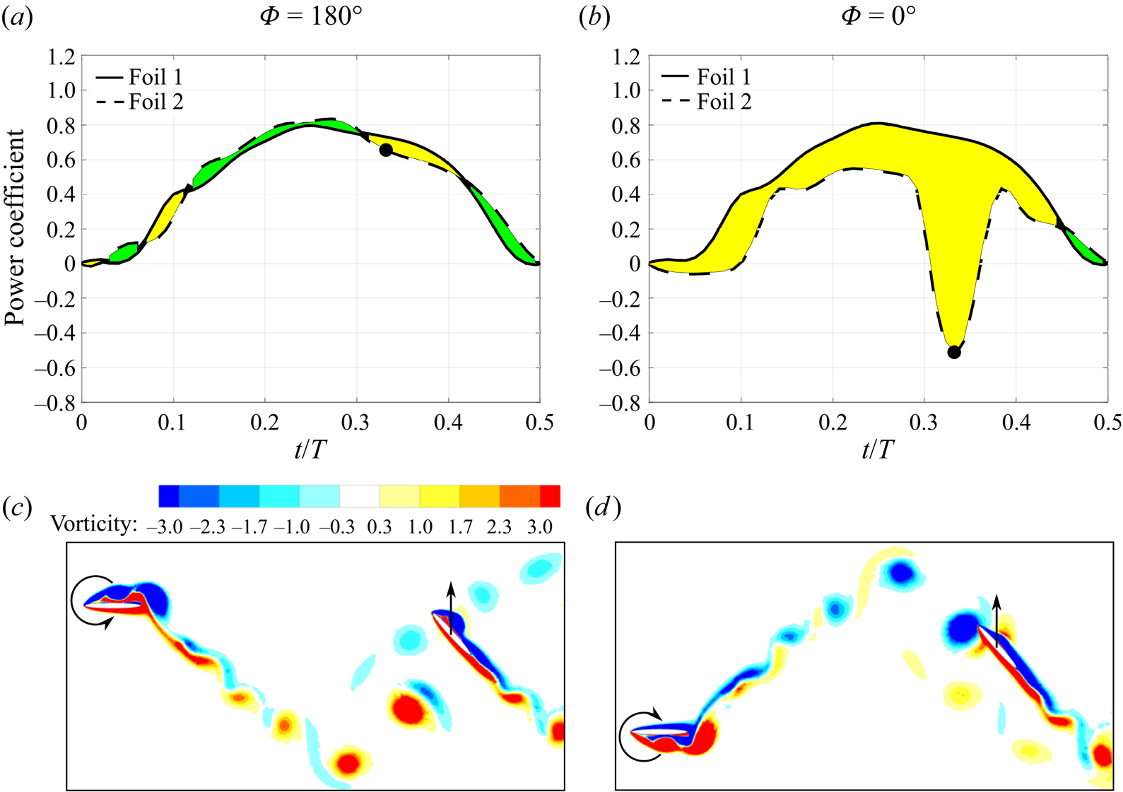
Figure 2. Analysis of vortex–foil interactions at wake phases $\varPhi =180^{\circ }$ and $\varPhi =0^{\circ }$ and foil parameters $f=0.10, h_o=1.0, \theta _o=55^{\circ }$. These phases illustrate the power contributions of the vortex gusts on the trailing foil when, for this case, there is a vortex-foil impingement ($\varPhi =0^{\circ }$) or vortex avoidance ($\varPhi =180^{\circ }$). The instantaneous vorticity flow fields are plotted at $t/T=0.33$ (black markers). (a) Similar power coefficient between foils, (b) power coefficient is affected by vortex–foil interactions, (c) vortex–foil avoidance and (d) vortex–foil impingement.

In contrast, figures 2(b) and 2(d) display the vorticity flow field and the power curve for the same foil kinematics but with a wake phase of $\varPhi =0^{\circ }$. In this configuration the foil intercepts a strong clockwise vortex on its upstroke, causing a large decrease in the instantaneous power coefficient at $t/T=0.33$. In contrast, if the vortex direction was counterclockwise, it may encourage the vortex formation over the downstream foil, and thus, generate a constructive vortex–foil interaction. The latter is typically found in staggered foil arrays (Kinsey & Dumas Reference Kinsey and Dumas2012) while the former is observed in tandem arrangements such as those investigated in this paper. Thus, the differences between these two curves, shaded yellow (negative) and green (positive), represent portions of the cycle where unsteady wake–foil interactions are influencing the power extraction.

3.1. Effective angle of attack in the presence of vortex disturbances

Using the wake velocity profiles described in § 2, an effective angle of attack is computed within the moving vortex window upstream of the trailing foil. First, an instantaneous velocity vector, $\boldsymbol {u^v}$, is computed by spatially averaging the velocity profile over $\Delta y$,

(3.1)\begin{equation} \boldsymbol{u^v}(\varPhi, t) = \frac{1}{\Delta y} \int_{y_{LE}(t+t^v) - \Delta y/2}^{y_{LE}(t+t^v) + \Delta y/2} \boldsymbol{u_w}(y, \varPhi, t) \, {{\rm d} y}.\end{equation}

Time is shifted by $t^v$,

(3.2)\begin{equation} t^v = \frac{S_x - x_w}{u_w}\end{equation}

to account for the convection time between the measured wake at $x=x_w$ and the trailing foil at $x=S_x$. The value of $y_{LE}(t+t^v)$ corresponds to the trailing foil's leading edge position at $t+t^v$, which is when the gust–foil interactions occur. Next, using the spatially averaged velocity within the vortex window, the effective angle of attack of the trailing foil, $\alpha ^v$, is calculated as

(3.3)\begin{equation} \alpha^v(\varPhi, t) = \theta(t) - \tan^{-1} \left(\frac{-\dot{h}(t) - v^v(\varPhi, t)}{u^v(\varPhi, t)}\right),\end{equation}

as illustrated by the velocity triangle and foil heave velocity in figure 3. Although the effective angle of attack is computed at $x=x_w$ it is assumed constant as the vortex convects from $x=x_w$ to $x=S_x$.

Figure 3. Effective angle of attack of the trailing foil in the presence of wake disturbances.

3.2. Introduction of a reference foil with an equivalent mean flow

To quantify the effects of the vortex gust on the trailing foil, an equivalent foil operating in a uniform flow with velocity $u_w$ is introduced as a reference foil illustrated in figure 4.

Figure 4. Effective angle of attack of the reference foil (no wake disturbances).

Thus, the kinematic parameters are now normalized by $u_w$ and are given as

(3.4a–c)\begin{equation} f^* = \frac{f}{u_w}, \quad h^*(t)=-h_{o} \cos(2{\rm \pi} f^* t), \quad \text{and} \quad \theta^*(t)=-\theta_{o} \sin(2{\rm \pi} f^* t),\end{equation}

where the $^*$ superscript denotes the reference foil. The effective angle of attack of the reference foil is defined by $\alpha ^*$,

(3.5)\begin{equation} \alpha^*(t) = \theta^*(t) - \tan^{-1} \left(\frac{-\dot{h}^*(t)}{u_w}\right).\end{equation}

The difference in effective angle of attack between the reference foil and the trailing foil is thus

(3.6)\begin{equation} \Delta \alpha (\varPhi, t) = \alpha^v(\varPhi, t) - \alpha^*(t),\end{equation}

which is an indication of the strength and direction of the unsteady flow in the near vicinity of the trailing foil.

The power coefficient for the reference foil is then calculated from $L^*$ and $\dot {h}^*$ as

(3.7)\begin{equation} C_p^*(t) = \frac{\dot{h}^*L^*(t)}{\tfrac{1}{2}\rho u_w^3 c}.\end{equation}

The power difference, $\Delta C_p$, between the gust–foil interaction and the equivalent reference foil is

(3.8)\begin{equation} \Delta C_p (\varPhi,t) = C_{p,2}(\varPhi,t) - C_p^*(t) = \frac{\dot{h}_2L_2(\varPhi, t)}{\tfrac{1}{2}\rho u_w^3 c} - \frac{\dot{h}^*L^*(t)}{\tfrac{1}{2}\rho u_w^3 c}.\end{equation}

To illustrate the relationship between these quantities, figure 5 shows $\Delta \alpha$ and $\Delta C_p$ profiles within the upstroke foil motion ($t/T=0\unicode{x2013}0.5$) for the wake phase $\varPhi =0^{\circ }$ with foil parameters $f=0.10$, $h_o=1.0$ and $\theta _o=55^{\circ }$. There is a significant $\Delta \alpha$ drop at approximately $t/T=0.33$, which translates to a vortex–foil interaction that is detrimental to the formation of vortices over the foil. This destructive interaction is also observed by a $\Delta C_p$ drop at approximately the same time.

Figure 5. Comparison between the difference in effective angle of attack and power coefficient at $\varPhi =0^{\circ }$ for foil parameters of $f=0.10$, $h_o=1.0$ and $\theta _o=55^{\circ }$.

3.3. Power prediction based on the effective angle of attack

Next, a relationship between $\Delta \alpha$ and $\Delta C_p$ is derived in order to complete the model for the energy harvesting efficiency of the trailing foil. Following from (3.8), which is the measured difference in power between the trailing foil and an equivalent reference foil, a modelled power difference is constructed utilizing input data from the upstream foil wake kinematics and the kinematics of the trailing foil. Since the effective angle of attack is proportional to the lift force on the foil (Biler et al. Reference Biler, Sedky, Jones, Saritas and Cetiner2021), the difference in power, $\Delta \widetilde {C_p}$, is modelled as

(3.9)\begin{equation} \Delta \widetilde{C_p}(\varPhi, t) = \beta (\varPhi)\left( \frac{\dot{h}_2 \alpha^v(\varPhi,t) - \dot{h}^*\alpha^*(t)}{\tfrac{1}{2}\rho u_w^3 c} \right ), \end{equation}

where the parameter $\beta$ represents a coefficient of proportionality between the power coefficient and effective angle of attack. Thus, a model of the time-dependent power coefficient of the trailing foil, $C_p^v$, as a function of wake phase $\phi$, can be constructed as

(3.10)\begin{equation} C_p^v(\varPhi, t) = C_p^* (t)+ \Delta \widetilde{C_p} (\varPhi, t).\end{equation}

The optimal value of $\beta$ (for each phase difference $\varPhi$) can be computed using data from two-foil simulations by minimizing the root-mean-square difference between the model and the instantaneous power profiles, demonstrated by the black lines in figure 6. For this subset of two-foil kinematics, $\beta$ peaks in the vicinity of $\varPhi =0^{\circ }$, coinciding with strong wake–foil interactions. In contrast, at phases closer to $180^{\circ }$, $\beta$ is generally smaller when the vortex–foil interactions are weaker. To maintain periodicity, a sinusoidal equation is fit to the data with a nonlinear least squares regression algorithm, generating a $\beta$ profile (blue curve in figure 6) given by

(3.11)\begin{equation} \beta(\varPhi) = 0.75\cos \left(\frac{\varPhi{\rm \pi}}{180} - 0.12{\rm \pi}\right)+0.41,\end{equation}

with $\varPhi$ given in degrees. A physical interpretation of the parameter $\beta$ is that it accounts for changes in the non-circulatory lift forces as the surrounding flow around the airfoil is modified by the presence of the vortex.

Figure 6. Optimal coefficient of proportionality, $\beta$, determined from two-foil data (black lines) and general $\beta$ profile implemented in the model (blue line).

4.1. Time-dependent power prediction

In figure 7 the instantaneous power coefficient developed by the model is compared against the computed power from a two-foil simulation, and compared against a reference foil of equivalent mean free-stream velocity. Whereas the simulation is the exact value, the reference foil represents the baseline power curve for a steady inlet flow. Three representative oscillation kinematics (cases A, B and C) are shown that span a range of $\alpha _{T/4}$ from $18^{\circ }$ to $28^{\circ }$. For each case, three phase angles are shown at $\varPhi =-30^{\circ }$, $0^{\circ }$ and $30^{\circ }$, representing the regime where vortex–foil interactions have the highest probability of occurring.

Figure 7. Comparison between power prediction ($C_p^v$), trailing foil ($C_{p,2}$) and reference foil ($C_p^*$) at three wake phases and configurations. Kinematics: Case A: $f=0.12$, $h_o=1.0$, $\theta _o=55^{\circ }$; Case B: $f=0.10$, $h_o=1.0$, $\theta _o=55^{\circ }$; Case C: $f=0.12$, $h_o=1.0$, $\theta _o=65^{\circ }$.

Across the data displayed, the occurrence of vortex–foil interactions in the trailing foil are well captured by the model, as indicated by the peaks and troughs in the power coefficient. Each wake–foil interaction may be classified as constructive or destructive depending on the vortex sign and positioning with respect to the foil (Ribeiro et al. Reference Ribeiro, Su, Guillaumin, Breuer and Franck2021). The reference foil (dark red line) is the baseline power for equivalent stroke kinematics without any unsteady vortex interaction. Thus, power achieved above the reference foil is described as a constructive vortex–foil interaction, whereas a power coefficient lower than the reference foil represents a destructive interaction. For the tandem configuration explored in this paper, the majority of the vortex–foil interactions are destructive, resulting in the computed and modelled power coefficient less than the reference foil. Most all of these vortex–foil interactions are captured by the model. However, there are instances where the timing and/or magnitude of the power is either over- or under-predicted. In the data shown, there are also two moments of constructive interaction in cases B and C at $\varPhi =-30^{\circ }$, identified by the instantaneous power coefficient surpassing that of the reference foil. The model captures this increase although the amplitude is under-predicted.

In general, when analysing the time-dependent power in each wake phase, the $\varPhi =0^{\circ }$ power prediction profiles are the closest to the simulation, representing where the maximum vortex–foil interaction is expected by the model. At wake phases just before ($\varPhi =-30^{\circ }$) or just after ($\varPhi =30^{\circ }$) the predicted power may have a time shift compared with the simulation as illustrated in case A at $\varPhi =-30^{\circ }$. This is due to the trailing foil interacting with the wake at an earlier time than the estimated vortex convection time.

These discrepancies between model and simulation tend to increase with higher values of $\alpha _{T/4}$, which are known to produce more chaotic wake structures (Ribeiro et al. Reference Ribeiro, Su, Guillaumin, Breuer and Franck2021). The amplitude deviation between model and simulation can be partially explained by the model considering a uniform $\beta$ profile for all kinematics. With stronger wake vortices, the effects of vortex–foil interactions are more apparent and, thus, the coefficient of proportionality between power and angle of attack may be higher than the $\beta$ given in the universal profile.

4.2. Time-averaged power coefficient as a function of wake phase

The time-averaged power coefficient is computed for the three representative cases and displayed in figure 8 as a function of wake phase. The dark red lines are the time-averaged power coefficient from the reference foil that is independent of wake phase since it assumes a steady flow. The $\alpha _{T/4}$ value increases from cases A to C and, thus, so does the strength of the vortex–foil interactions.

Figure 8. Time-averaged trailing foil power comparison between simulation and prediction model with respect to wake phase for three sets of foil kinematics. The dark red line corresponds to the mean power from the reference foil. Results are shown for (a) $\alpha _{T/4}=18^{\circ }$, (b) $\alpha _{T/4}=23^{\circ }$ and (c) $\alpha _{T/4}=28^{\circ }$.

Case A shows a sinusoidal power trend with respect to the wake phase, which occurs from the continuous and smooth interaction typically found in cases with similar values of relative angle of attack (Ribeiro & Franck Reference Ribeiro and Franck2022b). Overall, the model is able to capture the mean power trend at this low angle of attack with a slight under-prediction in magnitude. Similarly, a sinusoidal power variation is shown by the simulation data for case B. However, the model starts showing a more localized power variation around $\varPhi =0^{\circ }$ and a roughly constant power prediction at phase angles farther away from the main vortex interaction at $\varPhi =0^{\circ }$. Case C corresponds to a higher power of the reference foil since a stronger LEV and higher lift are found at the foil's mid-stroke position (Ribeiro, Frank & Franck Reference Ribeiro, Frank and Franck2020). Furthermore, a stronger and localized mean power variation is observed due to the more coherent wake vortices and stronger vortex–foil interactions compared with the other cases (Ribeiro et al. Reference Ribeiro, Su, Guillaumin, Breuer and Franck2021). For instance, as discussed by Ribeiro et al. (Reference Ribeiro, Su, Guillaumin, Breuer and Franck2021), the circulation of the primary vortex in case C is approximately $\varGamma /(U_\infty c) \approx 1.1$, which is higher than case B ($\varGamma /(U_\infty c) \approx 0.9$), and case A ($\varGamma /(U_\infty c) \approx 0.5$). For cases with leading foil kinematics at high relative angles of attack ($\alpha _{T/4} \geq 28^ {\circ }$), a TEV starts to form that also contributes to stronger wake–foil interactions. The strength of such vortices were previously correlated with $\alpha _{T/4}$ in the literature (Ribeiro et al. Reference Ribeiro, Su, Guillaumin, Breuer and Franck2021; Lee et al. Reference Lee, Simone, Su, Zhu, Ribeiro, Franck and Breuer2022). The more localized power variation explains the non-sinusoidal trend as the vortex–foil interactions are stronger and more localized compared with lower $\alpha _{T/4}$. The prediction model, however, is still able to capture this power trend shift as a function of wake phase and foil kinematics.

4.3. Model capabilities and limitations

The proposed wake–foil interaction model is able to predict the effects on instantaneous power coefficient as a result of constructive and destructive vortex–foil interactions. A single-foil simulation is utilized for input data, extracting the power coefficient of the baseline flow and the time-dependent wake data. Using this information, several proposed configurations and kinematics of the second foil can be easily modelled. These can be expanded beyond the tandem configurations currently proposed to include staggered configurations and various combinations of kinematic strokes.

Although the model predicts events when there is a direct impingement or weak interactions, there is a magnitude mismatch at wake phases close to $|\varPhi | \sim 90^{\circ }$, as seen in figure 8(b). A reason for the larger error at these phases is the failure of the vortex window to capture the entire wake disturbance that affects the power distribution. A potential solution may be to increase the vortex window size to include wake disturbances that have secondary effects on power generation. The vortex window size may become a limitation especially when considering cases with high $\alpha _{T/4}$ ($\alpha _{T/4} > 30^{\circ }$) since the vortex wakes in these cases contain not only LEVs but also TEVs and stronger secondary vortices that can affect power generation (Ribeiro et al. Reference Ribeiro, Su, Guillaumin, Breuer and Franck2021). For more details, Appendix B presents an error quantification between model and simulations based on the mean power coefficient.

Another potential improvement to the model is to account for the vortex trajectory and variation in vortex convection speed within the wake. It is assumed the primary vortex moves at a constant speed, however, our measurements have shown it does vary within the wake region. For this reason, the model relies on sampling the velocity field in close proximity (approximately 1 chord length upstream) to the second foil for the best estimate of the impact of the vortex on the local flow field. If the model incorporated a vortex trajectory and better convection speed, the sampled position could be moved upstream and provide more flexibility to the model.

A final consideration is that the proposed model only considers two-dimensional flows, which is often a good assumption for the high aspect ratio wings deployed for energy harvesting. Prior experimental work has shown that adding end plates maintains an approximately two-dimensional wake and improves the efficiency of the oscillating foils by mitigating tip losses (Kim et al. Reference Kim, Strom, Mandre and Breuer2017). Furthermore, these results have good agreement with simulations at a matching Reynolds number (Ribeiro et al. Reference Ribeiro, Frank and Franck2020). However, an extension to this model could incorporate a spanwise profile that accounts for the tip vortex and associated loss of lift and power.