


1. Introduction
Lock-released gravity currents (GC), with a denser fluid initially filling a reservoir and moving under gravity action immediately after a fast lift up of the gate, are widely studied since they model many geophysical flows such as avalanches, lava and pyroclastic flows, sea breezes and industrial flows (see Simpson Reference Simpson1997, for a general review). Numerous analytical and numerical approaches are discussed in literature (see Huppert Reference Huppert2006; Ungarish Reference Ungarish2009); furthermore, special laboratory experimental investigations were carried out, with the aim of improving the understanding of the phenomena providing verification and support to the theory.
Most of the studies of high-Reynolds number GC concern the propagation in a rectangular (or laterally unbounded) channel. However, in nature and practical applications the cross-section of the channel may show a more complicated geometrical shape, e.g. flow in a V-shaped valley, or in a circular/semicircular tunnel. It is therefore important to understand and model the effect of the non-rectangular cross-section geometry on the flow of high-Reynolds-number GC.
The investigation of this branch of GC has started recently, even though a seminal contribution was included in Benjamin (Reference Benjamin1968), as explained in § 5. In most cases a box model or a single-layer shallow-water (SW) model for lock-exchange problems is used (Monaghan et al. Reference Monaghan, Mériaux, Huppert and Monaghan2009b ; Marino & Thomas Reference Marino and Thomas2011; Zemach & Ungarish Reference Zemach and Ungarish2013) for Boussinesq systems; however, there are several limitations in the approximations of these models, which become severe whenever the dynamics of the ambient fluid cannot be neglected.
Ungarish (Reference Ungarish2013) developed a two-layer model for a high-Reynolds-number GC propagating after a dam-break in a horizontal channel with a general cross-section geometry. The method of characteristics is used to solve the problem, discerning new features (e.g. internal jumps or bores) with respect to the single-layer problem. The comparison of theory with some experiments performed in V- and power-law cross-section channels by Monaghan et al. (Reference Monaghan, Mériaux, Huppert and Monaghan2009b
) and by Marino & Thomas (Reference Marino and Thomas2011) is satisfactory as concerning the GC front speed of propagation $u_{N}$
(other quantities measured in those experiments were not amenable to clear-cut comparisons).
$u_{N}$
(other quantities measured in those experiments were not amenable to clear-cut comparisons).
Additional experiments in the V-shaped cross-section channel were recently reported by Ungarish, Mériaux & Kurz-Besson (Reference Ungarish, Mériaux and Kurz-Besson2014). This work can be considered a forerunner of the present investigation, because it considers comparisons with the same theoretical model, uses the same fluids with similar density contrasts, and the typical dimensions of the apparatus (length and height) are quite similar. However, there are significant qualitative differences concerning the range of coverage and quantitative differences concerning the effect of the geometry. In particular, the set-up of Ungarish et al. (Reference Ungarish, Mériaux and Kurz-Besson2014) did not allow measurements in the lock domain, and the number of tested systems was seven. In these respects, the present work is a significant extension because it investigates the flow in the lock, and considers 39 different combinations of the parameters with three different values of the relative densities of the two fluids. The circular cross-section geometry is obviously at significant difference with the V-triangle counterpart, and thus provides a test of the theory in independent new circumstances.
Our investigation is concerned with GC of constant density contrast with the ambient, called ‘homogeneous’ or ‘compositional driven’. The other related class, of ‘particle-driven’ GC in non-rectangular geometry, has also been the topic of recent investigations, see Monaghan et al. (Reference Monaghan, Mériaux, Huppert and Mansour2009a ), Mériaux & Kurz-Besson (Reference Mériaux and Kurz-Besson2012) and Nasr-Azadani & Meiburg (Reference Nasr-Azadani and Meiburg2014), with the focus on V-shaped channels. The sedimentation of particles produces major differences in many features of the flow-field, and therefore there are no overlaps between these studies and the present work.
To the aim of an experimental description of the current motion in the lock and downstream for a non-rectangular cross-section horizontal channel, and of a more stringent verification of the theory and of its limits, we designed and carried out a new set of experiments in a circular cross-section horizontal channel. We performed 10 experiments in a short-lock and 29 in a long-lock condition, for both full- and part-depth locks. The experiments in the short-lock configuration were used to analyse the various stages of the currents by measuring the GC front speed, whereas those in the long-lock configuration were used to measure the characteristics of the waves or of the bores moving upstream or downstream (after reflection at the lock back-wall) in the lock.
The adopted experimental techniques and analyses greatly improve the data accuracy and resolution in time and space. Our conclusion is that the two-layer SW model predicts well the overall dynamics of the system, with some quantitative discrepancies between theory and experiments largely due to the unavoidable influence of viscous effects (which were not included in the simplified model).
The paper is structured as follows. The theoretical model is briefly described in § 2. The laboratory experiments are detailed in § 3, with two subsections giving details on the experimental set-up and protocol, the instruments employed, the data elaboration procedure and the associated uncertainties. Section 4 contains the analysis and discussion of the experimental results for the motion in the lock and downstream, focusing attention on the kinematics of the bores/waves in the lock, and on $x_{V}$
, the distance of transition to viscous regime downstream. In § 5 there are some concluding remarks. The theoretical estimate of
$x_{V}$
, the distance of transition to viscous regime downstream. In § 5 there are some concluding remarks. The theoretical estimate of $x_{V}$
is derived in appendix A. Additional material (some calculations for the theoretical model, figures, videos and raw data of the experiments in the short-lock configuration) is available online as supplementary material at http://dx.doi.org/10.1017/jfm.2014.701.
$x_{V}$
is derived in appendix A. Additional material (some calculations for the theoretical model, figures, videos and raw data of the experiments in the short-lock configuration) is available online as supplementary material at http://dx.doi.org/10.1017/jfm.2014.701.
2. Theoretical model
The model is detailed in Ungarish (Reference Ungarish2013) and is briefly outlined here.
We consider (figure 1) the flow in a horizontal channel with cross-section characterized by the lower boundary consisting of a circular tube of radius $r^{\ast }$
, cut by the top plane at height
$r^{\ast }$
, cut by the top plane at height $H^{\ast }$
(the superscript asterisk denotes dimensional variables). The first relevant dimensionless geometrical parameter is
$H^{\ast }$
(the superscript asterisk denotes dimensional variables). The first relevant dimensionless geometrical parameter is ${\it\beta}=H^{\ast }/r^{\ast }~({\it\beta}\leqslant 2)$
. The full-circle cross-section is given by
${\it\beta}=H^{\ast }/r^{\ast }~({\it\beta}\leqslant 2)$
. The full-circle cross-section is given by ${\it\beta}=2$
, while a half-circle channel is represented by
${\it\beta}=2$
, while a half-circle channel is represented by ${\it\beta}=1$
;
${\it\beta}=1$
; ${\it\beta}\leqslant 1$
cases are roughly referred to as ‘semicircle’.
${\it\beta}\leqslant 1$
cases are roughly referred to as ‘semicircle’.
Figure 1. A schematic description of the lock release problem and a sketch of circle-segment cross-section for three values of the parameter ${\it\beta}$
. The point
${\it\beta}$
. The point $C$
is the centre of the circle, the cross area of the channel is
$C$
is the centre of the circle, the cross area of the channel is $A_{T}=A+A_{a}$
.
$A_{T}=A+A_{a}$
.
A denser fluid is initially at rest in a lock of length $x_{0}$
and height
$x_{0}$
and height $h_{0}$
, separated by a gate from the downstream channel, occupied by a lighter fluid. Hence, a second relevant parameter is
$h_{0}$
, separated by a gate from the downstream channel, occupied by a lighter fluid. Hence, a second relevant parameter is $H=H^{\ast }/h_{0}$
: the
$H=H^{\ast }/h_{0}$
: the $H=1$
case is usually referred to as ‘full-depth lock’ (and the initial stage as lock exchange); the other cases, with
$H=1$
case is usually referred to as ‘full-depth lock’ (and the initial stage as lock exchange); the other cases, with $H>1$
, as part-, or fractional-depth.
$H>1$
, as part-, or fractional-depth.
We introduce the density ratio parameter $R={\it\rho}_{a}/{\it\rho}_{c}$
of light to heavy fluid, and the reduced gravity
$R={\it\rho}_{a}/{\it\rho}_{c}$
of light to heavy fluid, and the reduced gravity $g^{\prime }=[({\it\rho}_{c}-{\it\rho}_{a})/{\it\rho}_{c}]g\equiv (1-R)g$
, where
$g^{\prime }=[({\it\rho}_{c}-{\it\rho}_{a})/{\it\rho}_{c}]g\equiv (1-R)g$
, where ${\it\rho}_{a}$
and
${\it\rho}_{a}$
and ${\it\rho}_{c}$
are the ambient fluid density and the current fluid density, respectively, and
${\it\rho}_{c}$
are the ambient fluid density and the current fluid density, respectively, and $g$
is the gravity acceleration.
$g$
is the gravity acceleration.
The reference velocity $U$
and time
$U$
and time $T$
are
$T$
are
 $$\begin{eqnarray}U=\left(g^{\prime }h_{0}\right)^{1/2};\quad T=x_{0}/U.\end{eqnarray}$$
The $x$
-lengths are scaled with
$x$
-lengths are scaled with $x_{0}$
, height and width with
$x_{0}$
, height and width with $h_{0}$
. Dimensionless variables are used hereafter unless stated otherwise.
$h_{0}$
. Dimensionless variables are used hereafter unless stated otherwise.
If the initial Reynolds number $\mathit{Re}_{0}=Uh_{0}/{\it\nu}_{c}$
, where
$\mathit{Re}_{0}=Uh_{0}/{\it\nu}_{c}$
, where ${\it\nu}_{c}$
is the kinematic viscosity of the current (dense) fluid, is sufficiently large, the propagation after the release at
${\it\nu}_{c}$
is the kinematic viscosity of the current (dense) fluid, is sufficiently large, the propagation after the release at $t=0$
is in the buoyancy-inertia (inviscid) regime. In addition, we assume that the current is thin (the aspect ratio
$t=0$
is in the buoyancy-inertia (inviscid) regime. In addition, we assume that the current is thin (the aspect ratio $h_{0}/x_{0}$
is small, practically less than one). Consequently the Navier–Stokes equations can be simplified into the SW approximation. The model provides the governing equations for the position of the interface
$h_{0}/x_{0}$
is small, practically less than one). Consequently the Navier–Stokes equations can be simplified into the SW approximation. The model provides the governing equations for the position of the interface $h$
measured from the bottom line of the channel, and the area-averaged velocity
$h$
measured from the bottom line of the channel, and the area-averaged velocity $u$
of the denser fluid, as functions of the independent variables
$u$
of the denser fluid, as functions of the independent variables $t,x$
for the circular cross-section. The equations are partial-differential of hyperbolic type. The cross-area occupied by the current is denoted by
$t,x$
for the circular cross-section. The equations are partial-differential of hyperbolic type. The cross-area occupied by the current is denoted by $A$
, the cross-area of the channel by
$A$
, the cross-area of the channel by $A_{T}$
and the area ratio by
$A_{T}$
and the area ratio by ${\it\varphi}=A/A_{T}$
(see figure 1). The calculations of
${\it\varphi}=A/A_{T}$
(see figure 1). The calculations of $A,A_{T},{\it\varphi}$
are performed by analytical formulae, which we present as supplementary material.
$A,A_{T},{\it\varphi}$
are performed by analytical formulae, which we present as supplementary material.
The GC front (or nose, for which we use the subscript $N$
) propagates with speed
$N$
) propagates with speed $u_{N}$
and the SW equations indicate that this is a discontinuity (shock) of height
$u_{N}$
and the SW equations indicate that this is a discontinuity (shock) of height $h_{N}$
. Therefore, at the GC front
$h_{N}$
. Therefore, at the GC front $x=x_{N}(t)$
we apply the extension of Benjamin’s (Reference Benjamin1968) jump condition to the present geometry (Ungarish Reference Ungarish2012),
$x=x_{N}(t)$
we apply the extension of Benjamin’s (Reference Benjamin1968) jump condition to the present geometry (Ungarish Reference Ungarish2012),
 $$\begin{eqnarray}u_{N}=\frac{1}{R^{1/2}}\mathit{Fr}h_{N}^{1/2};\quad \mathit{Fr}^{2}=\frac{2(1-{\it\varphi})}{1+{\it\varphi}}\left[1-{\it\varphi}+\frac{1}{hA_{T}}\int _{0}^{h}z\,f(z)\text{d}z\right],\end{eqnarray}$$
where the Froude number $\mathit{Fr}$
is calculated for
$\mathit{Fr}$
is calculated for $h=h_{N}$
and
$h=h_{N}$
and ${\it\varphi}={\it\varphi}_{N}$
, and
${\it\varphi}={\it\varphi}_{N}$
, and $f(z)=2[2(H/{\it\beta})z-z^{2}]^{1/2},~0\leqslant z\leqslant H$
, is the dimensionless width function for a circular cross-section, with all lengths being scaled by
$f(z)=2[2(H/{\it\beta})z-z^{2}]^{1/2},~0\leqslant z\leqslant H$
, is the dimensionless width function for a circular cross-section, with all lengths being scaled by $h_{0}$
.
$h_{0}$
.
The evaluations of $\mathit{Fr}$
involve integrals of the width function
$\mathit{Fr}$
involve integrals of the width function $f(z)$
, which can be easily obtained analytically as detailed in the supplementary material. Here
$f(z)$
, which can be easily obtained analytically as detailed in the supplementary material. Here $u_{N}$
is subcritical (or critical) when smaller than (or equal to) the speed
$u_{N}$
is subcritical (or critical) when smaller than (or equal to) the speed $c_{+}$
of the characteristic that reaches the GC front. Supercritical dam-break flows are non-physical.
$c_{+}$
of the characteristic that reaches the GC front. Supercritical dam-break flows are non-physical.
The SW model is self-contained and does not use adjustable constants. The analysis and solution discussed here are performed by reliable (‘exact’) mathematical tools: the methods of characteristics and similarity.
Some general insights for the circle cross-section can be derived and here a short summary is provided, with the full details presented in Ungarish (Reference Ungarish2013).
Consider the initial stage of propagation, after the sudden opening of the gate located at $x=0$
(a ‘dam-break’ situation). The analysis indicates that four types of flow can be distinguished, as sketched in figure 2. A disturbance propagates into the lock (reservoir). For
$x=0$
(a ‘dam-break’ situation). The analysis indicates that four types of flow can be distinguished, as sketched in figure 2. A disturbance propagates into the lock (reservoir). For $H<H_{crit}({\it\beta})$
the left-moving
$H<H_{crit}({\it\beta})$
the left-moving $c_{-}$
characteristics, which carry this perturbation into the stagnant fluid, intersect, and a moving jump appears. The solution of this jump provides the speed
$c_{-}$
characteristics, which carry this perturbation into the stagnant fluid, intersect, and a moving jump appears. The solution of this jump provides the speed $V_{f}$
(to the left, into the lock) and amplitude
$V_{f}$
(to the left, into the lock) and amplitude $h_{\ast }$
. For larger
$h_{\ast }$
. For larger $H$
, this perturbation is a rarefaction wave of speed
$H$
, this perturbation is a rarefaction wave of speed $c_{-}$
(and amplitude zero). We note in passing that there is no standard term for this flow-field component. Rottman & Simpson (Reference Rottman and Simpson1983) discussed this effect in the rectangular channel as ‘hydraulic drop, a type of internal bore’, and referred to the reflected jump simply as ‘bore’, but there are variations in other related papers. We shall use ‘bore’ for a jump moving to the left in the lock, and ‘wave’ for a smooth profile, defined also as ‘rarefaction wave’ if it is left-moving (generated by an expansion fan of the
$c_{-}$
(and amplitude zero). We note in passing that there is no standard term for this flow-field component. Rottman & Simpson (Reference Rottman and Simpson1983) discussed this effect in the rectangular channel as ‘hydraulic drop, a type of internal bore’, and referred to the reflected jump simply as ‘bore’, but there are variations in other related papers. We shall use ‘bore’ for a jump moving to the left in the lock, and ‘wave’ for a smooth profile, defined also as ‘rarefaction wave’ if it is left-moving (generated by an expansion fan of the $c_{-}$
characteristics). The bore and the rarefaction wave after reflection from the back-wall at
$c_{-}$
characteristics). The bore and the rarefaction wave after reflection from the back-wall at $x=-1$
are defined as ‘reflected bore’ and ‘reflected wave’.
$x=-1$
are defined as ‘reflected bore’ and ‘reflected wave’.
Figure 2. Schematic description of the types of flow fields. (a) Type 1: rarefaction wave into the reservoir (position $L$
) and subcritical GC front (position
$L$
) and subcritical GC front (position $N$
). (b) Type 2: moving jump (bore) at position
$N$
). (b) Type 2: moving jump (bore) at position $L$
, subcritical GC front. (c) Type 3: moving jump (bore) at position
$L$
, subcritical GC front. (c) Type 3: moving jump (bore) at position $L$
, critical GC front. (d) Type 4: same as type 3, with additional stationary jump at position
$L$
, critical GC front. (d) Type 4: same as type 3, with additional stationary jump at position $x=0$
. The type 4 flow is a rare occurrence, for
$x=0$
. The type 4 flow is a rare occurrence, for ${\it\beta}$
very close to 2 and
${\it\beta}$
very close to 2 and $H$
very close to 1 only. Here
$H$
very close to 1 only. Here $z$
is scaled with
$z$
is scaled with $h_{0},x$
with
$h_{0},x$
with $x_{0}$
. Point
$x_{0}$
. Point $L$
denotes the transition from the reservoir to the activated (moving) domain,
$L$
denotes the transition from the reservoir to the activated (moving) domain, $N$
the GC front on the opposite boundary of the activated domain;
$N$
the GC front on the opposite boundary of the activated domain; $M$
denotes the left boundary of the core, and
$M$
denotes the left boundary of the core, and $Q$
the left boundary of the expansion domain following the GC front (when present).
$Q$
the left boundary of the expansion domain following the GC front (when present).
The speed and amplitude of the wave into the reservoir are predicted to be time-independent until the wave hits the back-wall $x=-1$
. Then, reflection occurs: the left-moving bore turns into a reflected bore with a new speed
$x=-1$
. Then, reflection occurs: the left-moving bore turns into a reflected bore with a new speed $V_{b}$
(to the right) and amplitude
$V_{b}$
(to the right) and amplitude $h_{\ast \ast }$
; the rarefaction wave changes direction (to the right). The theory provides the values of these effects. We note that the reflected bore/wave is not expected to move with constant speed (actually, it is expected to accelerate to a speed larger than
$h_{\ast \ast }$
; the rarefaction wave changes direction (to the right). The theory provides the values of these effects. We note that the reflected bore/wave is not expected to move with constant speed (actually, it is expected to accelerate to a speed larger than $u_{N}$
while the GC front moves with the constant
$u_{N}$
while the GC front moves with the constant $u_{N}$
).
$u_{N}$
).
In realistic flows the interface between the current and the ambient is not sharp due to the presence of unavoidable local vortices, viscous smearing and mixing. Moreover, at the bottom and sidewalls the realistic current is restricted by no-slip condition. Consequently, a global comparison of interfaces is a quite inconclusive test for the theoretical prediction. Nevertheless, we expect (and confirm later) that some salient properties, such as the speed of propagation and the amplitude of the disturbances into the lock, and the speed of propagation of the current, can be measured with sufficient accuracy for making useful comparisons with the theoretical predictions.
The SW theory predicts that the front (nose) of the current displays an initial ‘slumping’ stage of propagation with constant velocity $u_{N}$
, over a significant distance
$u_{N}$
, over a significant distance $x_{s}$
. The value of the slumping
$x_{s}$
. The value of the slumping $u_{N}$
can be obtained analytically.
$u_{N}$
can be obtained analytically.
At some distance $x_{s}$
(when the reflected bore/wave reaches the GC front) the inviscid current begins to decelerate, and undergoes transition to a self-similar stage of propagation
$x_{s}$
(when the reflected bore/wave reaches the GC front) the inviscid current begins to decelerate, and undergoes transition to a self-similar stage of propagation $x_{N}(t)\sim Kt^{3/4}$
, with
$x_{N}(t)\sim Kt^{3/4}$
, with $K$
being a constant. There is no simple analytical prediction for
$K$
being a constant. There is no simple analytical prediction for $x_{s}$
, but a qualitative analysis indicates that
$x_{s}$
, but a qualitative analysis indicates that $x_{s}$
decreases with
$x_{s}$
decreases with $H$
, and is approximately 3 for large
$H$
, and is approximately 3 for large $H$
(deep current). Although the transition from slumping to self-similar stage is not sharp, we can attempt to detect this effect in our experiments. To this end we must use long channels (in terms of lock-lengths). In the self-similar stage the speed and thickness decrease with
$H$
(deep current). Although the transition from slumping to self-similar stage is not sharp, we can attempt to detect this effect in our experiments. To this end we must use long channels (in terms of lock-lengths). In the self-similar stage the speed and thickness decrease with $t$
, and the typical inertia term
$t$
, and the typical inertia term $u_{N}^{2}/x_{N}$
decays significantly. The current becomes prone to viscous influence.
$u_{N}^{2}/x_{N}$
decays significantly. The current becomes prone to viscous influence.
The SW model becomes invalid after the current spreads to $x_{V}$
, where the viscous forces become influential. The estimate (appendix A) is
$x_{V}$
, where the viscous forces become influential. The estimate (appendix A) is
 $$\begin{eqnarray}x_{V}=0.5\left[\mathit{Re}_{0}(h_{0}/x_{0})\right]^{3/8}.\end{eqnarray}$$
We shall attempt to verify this prediction in our experiments.
For simplicity of analysis, we shall use the Boussinesq SW results. The Boussinesq approximation relative error is approximately $0.5(1-R)$
, which in our experiments was typically 2–5 %, in the range of the experimental uncertainties.
$0.5(1-R)$
, which in our experiments was typically 2–5 %, in the range of the experimental uncertainties.
3. Laboratory experiments
3.1. Experimental set-up
Figure 3 shows the schematic description of the experimental apparatus and its main components.
Figure 3. Schematic description of the experimental apparatus.
The experiments were carried out in a polymethyl methacrylate (PMMA, a transparent thermoplastic) circular tube with internal radius $r^{\ast }=9.5~\text{cm}$
in which a guillotine gate was inserted to separate the upstream portion (the lock) from the downstream channel. In different experiments, the length of the lock
$r^{\ast }=9.5~\text{cm}$
in which a guillotine gate was inserted to separate the upstream portion (the lock) from the downstream channel. In different experiments, the length of the lock $x_{0}$
varied between 6, 15 or 100 cm, while the length of the downstream pipe was 200, 400 or 600 cm. The horizontality of the tube was checked with an electronic spirit level accurate to
$x_{0}$
varied between 6, 15 or 100 cm, while the length of the downstream pipe was 200, 400 or 600 cm. The horizontality of the tube was checked with an electronic spirit level accurate to $0.1^{\circ }$
.
$0.1^{\circ }$
.
The ambient fluid, of density ${\it\rho}_{a}$
, was tap water treated with a softener; the current fluid, of density
${\it\rho}_{a}$
, was tap water treated with a softener; the current fluid, of density ${\it\rho}_{c}$
, was salt water added with aniline dye to enable flow visualization. In the set-up of the experiments, the tube was first partially filled with the fresh water and subsequently the saline fluid was gently added near the bottom of the lock, with the gate lifted but leaving an upper connection between the lock and the rest of the tube (for the specific gate adopted, completely lifted indicates that the lock and the rest of the channel are disconnected).
${\it\rho}_{c}$
, was salt water added with aniline dye to enable flow visualization. In the set-up of the experiments, the tube was first partially filled with the fresh water and subsequently the saline fluid was gently added near the bottom of the lock, with the gate lifted but leaving an upper connection between the lock and the rest of the tube (for the specific gate adopted, completely lifted indicates that the lock and the rest of the channel are disconnected).
This set-up allowed us to consider different height ratios $H$
of ambient to lock. The levels of the fluids were obtained by carefully observing the interface, avoiding parallax errors, and measuring the position of the meniscus by means of a ruler stuck to the tube. After filling the lock and the downstream tube, the temperature of both fluids was measured by using a
$H$
of ambient to lock. The levels of the fluids were obtained by carefully observing the interface, avoiding parallax errors, and measuring the position of the meniscus by means of a ruler stuck to the tube. After filling the lock and the downstream tube, the temperature of both fluids was measured by using a $0.02\,^{\circ }\text{C}$
accurate thermometer, waiting for the temperature to reach an equilibrium before starting the experiment. In most experiments the temperature was between 17 and
$0.02\,^{\circ }\text{C}$
accurate thermometer, waiting for the temperature to reach an equilibrium before starting the experiment. In most experiments the temperature was between 17 and $18\,^{\circ }\text{C}$
, and the measured value was used for the computation of the kinematic viscosity of the current fluid. The density of the current fluid was measured by using a
$18\,^{\circ }\text{C}$
, and the measured value was used for the computation of the kinematic viscosity of the current fluid. The density of the current fluid was measured by using a $10^{-3}~\text{g}~\text{cm}^{-3}$
accurate pycnometer.
$10^{-3}~\text{g}~\text{cm}^{-3}$
accurate pycnometer.
By varying the salinity, densities of the intruding fluid equal to $1.042,\,1.085,$ $1.117~\text{g}~\text{cm}^{-3}$
were obtained, resulting in density ratios
$1.117~\text{g}~\text{cm}^{-3}$
were obtained, resulting in density ratios $1-R=({\it\rho}_{c}-{\it\rho}_{a})/{\it\rho}_{c}$
of
$1-R=({\it\rho}_{c}-{\it\rho}_{a})/{\it\rho}_{c}$
of $4.1,\;7.9,\;10.6\,\%$
, respectively. These density differences render the flow in the Boussinesq regime. The corresponding kinematic viscosities were
$4.1,\;7.9,\;10.6\,\%$
, respectively. These density differences render the flow in the Boussinesq regime. The corresponding kinematic viscosities were $1.17\times 10^{-2},\,1.30\times 10^{-2},\,1.40\times 10^{-2}~\text{cm}^{2}~\text{s}^{-1}$
. Each experiment was recorded by several photo cameras with a data rate up to 2 f.p.s. (frames per second) and by a full HD video camera at 25 f.p.s. controlled by a PC. The start of the acquisition was triggered by a micro switch closed by the gate, with the time
$1.17\times 10^{-2},\,1.30\times 10^{-2},\,1.40\times 10^{-2}~\text{cm}^{2}~\text{s}^{-1}$
. Each experiment was recorded by several photo cameras with a data rate up to 2 f.p.s. (frames per second) and by a full HD video camera at 25 f.p.s. controlled by a PC. The start of the acquisition was triggered by a micro switch closed by the gate, with the time $t=0$
corresponding to the complete opening. It took approximately 0.8 s to completely open the gate with a full-depth release system,
$t=0$
corresponding to the complete opening. It took approximately 0.8 s to completely open the gate with a full-depth release system, $H=1$
, and
$H=1$
, and ${\it\beta}=2$
, and less for a partial-depth release system.
${\it\beta}=2$
, and less for a partial-depth release system.
Video image analysis was used to detect the GC front position and the profiles in the lock. A grid was stuck to the bottom of the tube and could be observed reflected in mirrors providing a bottom view. Another grid was stuck to the side of the lock and could be directly observed by a high-resolution photo camera. A Matlab® proprietary software for calibrating the camera allowed the evaluation of the function to convert the pixel coordinates to metric coordinates, including the correction for lens distortion and curvature of the tube. The resolution was usually better than $0.01~\text{cm}/\text{pixel}$
, with an overall uncertainty less than 0.2 cm.
$0.01~\text{cm}/\text{pixel}$
, with an overall uncertainty less than 0.2 cm.
High-frequency neon lights were used to provide a uniform and stable illumination, in order to improve the automatic detection of the interface between the ambient fluid and the current. Since the cameras had restricted intervals of movements, subsequent frames were not perfectly overlapped and it was necessary to resize the frames and correct the pixel position with a second Matlab® proprietary software. As shown in figure 4, images were generally of good quality; the interface between the two fluids was observed to be quite sharp especially when the density difference was larger ( $1-R=7.9,\;10.6\,\%$
).
$1-R=7.9,\;10.6\,\%$
).
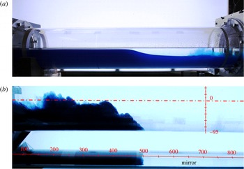
Figure 4. Pictures of the motion (left to right) in the lock (a) and downstream (b). Experiment 2, ${\it\beta}=1$
,
${\it\beta}=1$
, $H=1.1$
,
$H=1.1$
, $({\it\rho}_{c}-{\it\rho}_{a})/{\it\rho}_{c}=4.1\,\%$
,
$({\it\rho}_{c}-{\it\rho}_{a})/{\it\rho}_{c}=4.1\,\%$
, $\mathit{Re}_{0}=13.8\times 10^{3}$
, type 3 profile (see figure 2).
$\mathit{Re}_{0}=13.8\times 10^{3}$
, type 3 profile (see figure 2).
The motion of the current was recorded over a length of 200 or 400 cm downstream for a lock length $x_{0}=100~\text{cm}$
, and over 600 cm for
$x_{0}=100~\text{cm}$
, and over 600 cm for $x_{0}=15~\text{cm}$
or
$x_{0}=15~\text{cm}$
or $x_{0}=6~\text{cm}$
. The motion in the lock was recorded only in the experiments with
$x_{0}=6~\text{cm}$
. The motion in the lock was recorded only in the experiments with $x_{0}=100~\text{cm}$
. In the analysis of the downstream flow, the interface between the current and the ambient fluid was detected and averaged over a 1.0 cm wide strip across the bottom of the pipe, with a time step coincident with the time interval between two subsequent frames (0.5–1 s for photo cameras,
$x_{0}=100~\text{cm}$
. In the analysis of the downstream flow, the interface between the current and the ambient fluid was detected and averaged over a 1.0 cm wide strip across the bottom of the pipe, with a time step coincident with the time interval between two subsequent frames (0.5–1 s for photo cameras, $1/25~\text{s}$
for the video camera) or a multiple of said time interval for cross-sections far from the lock gate, where the current had already decelerated. For this reason, the data rate in the recorded time series of the front position is variable within the same experiment (these data are available as supplementary material for the 10 experiments in the short-lock configuration).
$1/25~\text{s}$
for the video camera) or a multiple of said time interval for cross-sections far from the lock gate, where the current had already decelerated. For this reason, the data rate in the recorded time series of the front position is variable within the same experiment (these data are available as supplementary material for the 10 experiments in the short-lock configuration).
The video camera was triggered with an LED controlled by the PC and visible in the FOV (field of view), giving a negligible delay with respect to the micro switch signal. The photo cameras (Canon EOS, reflex models) had a systematic delay of less than 0.1 s in acquiring the images, correspondent to the time of reversal of the internal mirror before the opening of the shutter. The FOVs of the photo cameras and of the video camera were overlapped in order to detect the correct timing of the images by comparing the two records. Some gaps in the time series were due to the presence of struts and supports of the tube which hid the view.
We performed two sets of experiments focused, respectively, on: (i) the motion in the lock; (ii) the motion of the GC front and the transition between the inertial-buoyancy phase (slumping and self-similar) and the viscous-buoyancy phase.
Figure 5. The shape of the left-moving profiles for different values of $H$
and for
$H$
and for $1-R=7.9\,\%$
. The experiment with
$1-R=7.9\,\%$
. The experiment with $H=1.0$
refers to
$H=1.0$
refers to ${\it\beta}=2$
(Experiment 34) whereas the other three experiments refer to
${\it\beta}=2$
(Experiment 34) whereas the other three experiments refer to ${\it\beta}=1.5$
(Experiments 16, 18 and 20). The type is in figure 2.
${\it\beta}=1.5$
(Experiments 16, 18 and 20). The type is in figure 2.
3.2. The uncertainty in measurements and in parameters
Here we estimate the experimental uncertainties affecting the problem parameters. The mass density of the fluids was measured with a pycnometer having an uncertainty of $10^{-3}~\text{g}~\text{cm}^{-3}$
, hence the parameter
$10^{-3}~\text{g}~\text{cm}^{-3}$
, hence the parameter $R={\it\rho}_{a}/{\it\rho}_{c}$
had an uncertainty
$R={\it\rho}_{a}/{\it\rho}_{c}$
had an uncertainty ${\rm\Delta}R/R=0.2\,\%$
. The level of the fluids was detected with an accuracy of 0.1 cm, inducing a relative uncertainty
${\rm\Delta}R/R=0.2\,\%$
. The level of the fluids was detected with an accuracy of 0.1 cm, inducing a relative uncertainty ${\rm\Delta}H/H\leqslant 6\,\%$
and
${\rm\Delta}H/H\leqslant 6\,\%$
and ${\rm\Delta}{\it\beta}/{\it\beta}\leqslant 2.5\,\%$
. The velocity and the time scales had an uncertainty
${\rm\Delta}{\it\beta}/{\it\beta}\leqslant 2.5\,\%$
. The velocity and the time scales had an uncertainty ${\rm\Delta}U/U\leqslant 2.5\,\%$
and
${\rm\Delta}U/U\leqslant 2.5\,\%$
and ${\rm\Delta}T/T\leqslant 3\,\%$
, respectively, and
${\rm\Delta}T/T\leqslant 3\,\%$
, respectively, and $\mathit{Re}_{0}$
had an uncertainty
$\mathit{Re}_{0}$
had an uncertainty ${\rm\Delta}\mathit{Re}_{0}/\mathit{Re}_{0}\leqslant 8\,\%$
. These relative uncertainties were used to derive the error affecting the experimental results presented in the sequel.
${\rm\Delta}\mathit{Re}_{0}/\mathit{Re}_{0}\leqslant 8\,\%$
. These relative uncertainties were used to derive the error affecting the experimental results presented in the sequel.
4. Results and discussion
4.1. The motion in the lock
The motion in the lock was analysed by performing 29 experiments using the long lock configuration of length $x_{0}=100~\text{cm}$
. Different combinations of geometrical parameters were assembled, resulting in three different values of
$x_{0}=100~\text{cm}$
. Different combinations of geometrical parameters were assembled, resulting in three different values of ${\it\beta}=H^{\ast }/r^{\ast }$
equal to
${\it\beta}=H^{\ast }/r^{\ast }$
equal to $1$
,
$1$
, $1.5$
or
$1.5$
or $2$
, and in a range of height ratios
$2$
, and in a range of height ratios $H=H^{\ast }/h_{0}$
of ambient to lock varying between 1 and 3. These were combined with the three density ratios
$H=H^{\ast }/h_{0}$
of ambient to lock varying between 1 and 3. These were combined with the three density ratios $1-R=({\it\rho}_{c}-{\it\rho}_{a})/{\it\rho}_{c}=4.1,\;7.9,\;10.6\,\%$
. In all experiments the initial Reynolds number
$1-R=({\it\rho}_{c}-{\it\rho}_{a})/{\it\rho}_{c}=4.1,\;7.9,\;10.6\,\%$
. In all experiments the initial Reynolds number $\mathit{Re}_{0}$
was larger than 3000, ensuring the existence of an inviscid regime for several lock lengths before evolving gradually into a viscous regime. Table 1 summarizes the main parameters of the experiments.
$\mathit{Re}_{0}$
was larger than 3000, ensuring the existence of an inviscid regime for several lock lengths before evolving gradually into a viscous regime. Table 1 summarizes the main parameters of the experiments.
Table 1. Parameters of the experiments in the long lock configuration. The internal radius of the cross-section is $r^{\ast }=9.5~\text{cm}$
, the length of the lock is
$r^{\ast }=9.5~\text{cm}$
, the length of the lock is $x_{0}=100~\text{cm}$
. Here
$x_{0}=100~\text{cm}$
. Here $1-R=({\it\rho}_{c}-{\it\rho}_{a})/{\it\rho}_{c},g^{\prime }=(1-R)g$
is the reduced gravity,
$1-R=({\it\rho}_{c}-{\it\rho}_{a})/{\it\rho}_{c},g^{\prime }=(1-R)g$
is the reduced gravity, $\mathit{Re}_{0}=Uh_{0}/{\it\nu}_{c}$
is the Reynolds number with
$\mathit{Re}_{0}=Uh_{0}/{\it\nu}_{c}$
is the Reynolds number with ${\it\nu}_{c}$
the kinematic viscosity of the denser fluid,
${\it\nu}_{c}$
the kinematic viscosity of the denser fluid, $U=\sqrt{g^{\prime }h_{0}}$
and
$U=\sqrt{g^{\prime }h_{0}}$
and $T=x_{0}/U$
are the velocity and the time scale, respectively. The type refers to the classification sketched in figure 2. The superscript
$T=x_{0}/U$
are the velocity and the time scale, respectively. The type refers to the classification sketched in figure 2. The superscript $a$
in the first column indicates that a video is available as supplementary material.
$a$
in the first column indicates that a video is available as supplementary material.
A qualitative analysis of the current profile in the lock was first conducted. Figure 5 shows the profile for various values of $H$
and
$H$
and $1-R=7.9\,\%$
. In all cases a bore is predicted (see figure 2). The photographs were taken with the head of the upstream moving current located roughly in the same position within the lock. The structure of the profile depends on the relative velocity between the two currents (the denser fluid current below and the lighter fluid current), which increases for decreasing
$1-R=7.9\,\%$
. In all cases a bore is predicted (see figure 2). The photographs were taken with the head of the upstream moving current located roughly in the same position within the lock. The structure of the profile depends on the relative velocity between the two currents (the denser fluid current below and the lighter fluid current), which increases for decreasing $H$
. While for
$H$
. While for $H\geqslant 1.5$
the profile is regular and smooth and no instabilities develop at the interface, for
$H\geqslant 1.5$
the profile is regular and smooth and no instabilities develop at the interface, for $1.1<H<1.5$
some billows are present behind the smooth head of the current at a distance progressively reduced for decreasing
$1.1<H<1.5$
some billows are present behind the smooth head of the current at a distance progressively reduced for decreasing $H$
. A strong mixing is also evident behind the billows. For
$H$
. A strong mixing is also evident behind the billows. For $H=1$
the current becomes turbulent at the very beginning of the motion, and its shape is strongly affected by turbulent mixing. This sequence is typical of all tests, with minor differences for different values of
$H=1$
the current becomes turbulent at the very beginning of the motion, and its shape is strongly affected by turbulent mixing. This sequence is typical of all tests, with minor differences for different values of $R$
. When the density difference between the currents is smaller, mixing is enhanced.
$R$
. When the density difference between the currents is smaller, mixing is enhanced.
The corresponding profiles after reflection from the back-wall of the lock are shown in figure 6. It is noted that the observed shape depends on the evolution of the left-moving profile. For $H=1.5$
some billows develop near the gate; these become more evident with the increase of
$H=1.5$
some billows develop near the gate; these become more evident with the increase of $\mathit{Re}_{0}$
. Moreover, it is observed that for
$\mathit{Re}_{0}$
. Moreover, it is observed that for $H=1.5$
a significant portion of the interface does not show any appreciable mixing, while for
$H=1.5$
a significant portion of the interface does not show any appreciable mixing, while for $H\leqslant 1.1$
the mixing affects all of the lock length.
$H\leqslant 1.1$
the mixing affects all of the lock length.
Figure 6. The shape of the right-moving reflected bore/wave. Caption as in figure 5.
The predicted stationary jump at $x=0$
for type 4 flow (full-circle full-depth geometry
$x=0$
for type 4 flow (full-circle full-depth geometry ${\it\beta}=2$
,
${\it\beta}=2$
, $H=1$
, see figure 2
d), could not be observed because of the limitations of the experimental set-up. Since the jump is a stationary height change of small amplitude (4.8 % of the diameter), its detection among the unavoidable moving eddies and billows at the interface is a difficult task, which is left for future experiments.
$H=1$
, see figure 2
d), could not be observed because of the limitations of the experimental set-up. Since the jump is a stationary height change of small amplitude (4.8 % of the diameter), its detection among the unavoidable moving eddies and billows at the interface is a difficult task, which is left for future experiments.
To provide quantitative results, the detection of the profile of the current was conducted through the image analysis of the frames captured at a constant time interval. Since the algorithm detects the boundary between the fluids according to a threshold value of the greyscale level, an adequate accuracy and repeatability could be obtained only with uniform lightening. Choosing a proper threshold allowed us to distinguish between the core of the current and the billows or eddies generally present for currents with high $\mathit{Re}_{0}$
. A typical sequence of automatically detected profiles is shown in figure 7. Notably, their shape was conserved upon translation, indicating a progressive permanent profile. However, it is difficult to visually detect the jump, and in practice we analysed the second derivative of the instantaneous profile in order to calculate where a sharp change of inclination takes place. The location of the change has been considered as the start/end section of the moving jump.
$\mathit{Re}_{0}$
. A typical sequence of automatically detected profiles is shown in figure 7. Notably, their shape was conserved upon translation, indicating a progressive permanent profile. However, it is difficult to visually detect the jump, and in practice we analysed the second derivative of the instantaneous profile in order to calculate where a sharp change of inclination takes place. The location of the change has been considered as the start/end section of the moving jump.
Once the profiles of the denser current moving in the lock were detected, the speed and the height of the bore/wave could be readily computed.
Figure 8(a) shows the experimental speed $V_{f}$
of the bore moving to the left in the lock, compared with the theoretical prediction. The value reported for each experiment is the average speed of experimental profiles (i.e. the mean horizontal translation of the interface profile detected in two subsequent frames, divided by the time interval, typically 0.5 s, separating the frames). In most experiments, 5–6 pairs of profiles were available for the averaging procedure, since those recorded immediately after the gate opening were still influenced by the gate movement; in Experiment 1 the video camera was used to record the lock motion, and with a time interval between frames of
$V_{f}$
of the bore moving to the left in the lock, compared with the theoretical prediction. The value reported for each experiment is the average speed of experimental profiles (i.e. the mean horizontal translation of the interface profile detected in two subsequent frames, divided by the time interval, typically 0.5 s, separating the frames). In most experiments, 5–6 pairs of profiles were available for the averaging procedure, since those recorded immediately after the gate opening were still influenced by the gate movement; in Experiment 1 the video camera was used to record the lock motion, and with a time interval between frames of $1/25~\text{s}$
, several tens of profiles were available. In a number of cases, the experimental profiles were strongly distorted by billows and curls, with a strong turbulent diffusion able to smooth out the jump; these profiles could not be reliably used and were discarded. The speed estimated with the aforementioned procedure is not constant, but generally increases immediately after the gate opening, reaches a maximum and then decreases. The experimental speed is lower than its theoretical counterpart, with a very good agreement at low
$1/25~\text{s}$
, several tens of profiles were available. In a number of cases, the experimental profiles were strongly distorted by billows and curls, with a strong turbulent diffusion able to smooth out the jump; these profiles could not be reliably used and were discarded. The speed estimated with the aforementioned procedure is not constant, but generally increases immediately after the gate opening, reaches a maximum and then decreases. The experimental speed is lower than its theoretical counterpart, with a very good agreement at low $H$
and a discrepancy of approximately 25 % for
$H$
and a discrepancy of approximately 25 % for $H=3$
. The trend that the speed increases with
$H=3$
. The trend that the speed increases with $H$
is consistent with the theory.
$H$
is consistent with the theory.
Figure 7. Detection of the interface profiles in the lock with a time step of 0.5 s. Experiment 3 with ${\it\beta}=1$
,
${\it\beta}=1$
, $H=1.1$
,
$H=1.1$
, $1-R=10.6\,\%$
,
$1-R=10.6\,\%$
, $\mathit{Re}_{0}=18.4\times 10^{3}$
.
$\mathit{Re}_{0}=18.4\times 10^{3}$
.
Figure 8. Velocity $V_{f}$
(a) and height
$V_{f}$
(a) and height $h_{\ast }$
(b) of the bore or rarefaction wave in the lock as a function of
$h_{\ast }$
(b) of the bore or rarefaction wave in the lock as a function of $H$
for
$H$
for ${\it\beta}=1,\,1.5,\,2.0$
. For the rarefaction wave,
${\it\beta}=1,\,1.5,\,2.0$
. For the rarefaction wave, $h_{\ast }=0$
. Symbols and lines represent experimental results and theoretical predictions, respectively. The type of profile is indicated as t2–t4. The error bars indicate one standard deviation.
$h_{\ast }=0$
. Symbols and lines represent experimental results and theoretical predictions, respectively. The type of profile is indicated as t2–t4. The error bars indicate one standard deviation.
Figure 8(b) shows the height of the left-moving bore $h_{\ast }$
. For
$h_{\ast }$
. For $H>2$
(approximately) there is no jump, in agreement with the theory; however, the measured height of the rarefaction wave can be compared with the difference
$H>2$
(approximately) there is no jump, in agreement with the theory; however, the measured height of the rarefaction wave can be compared with the difference $(1-h_{X}),h_{X}$
being the height of the current at the gate (
$(1-h_{X}),h_{X}$
being the height of the current at the gate ( $x=0$
). Since the experimental measurements of the profiles start at
$x=0$
). Since the experimental measurements of the profiles start at $x\approx -20~\text{cm}$
, we expect that the measured height is always less than
$x\approx -20~\text{cm}$
, we expect that the measured height is always less than $(1-h_{X})$
. The results indicate that for Experiments 8 and 11,
$(1-h_{X})$
. The results indicate that for Experiments 8 and 11, $h_{e-w}=0.316\pm 0.03<0.465$
(theoretical SW evaluation), and for Experiments 39 and 40,
$h_{e-w}=0.316\pm 0.03<0.465$
(theoretical SW evaluation), and for Experiments 39 and 40, $h_{e-w}=0.347\pm 0.01<0.482$
, where
$h_{e-w}=0.347\pm 0.01<0.482$
, where $h_{e-w}$
is the measured height of the rarefaction wave in a type 1 profile. This is not a sharp comparison between experiments and theory, but the observed consistency supports the model.
$h_{e-w}$
is the measured height of the rarefaction wave in a type 1 profile. This is not a sharp comparison between experiments and theory, but the observed consistency supports the model.
For a deeper understanding of the prediction of speed of the bore or rarefaction wave, we depict in figure 9 the relative error against $\mathit{Re}_{0}$
(figure 9
a) and against
$\mathit{Re}_{0}$
(figure 9
a) and against $\mathit{Re}_{0}(h_{0}/x_{0})$
(figure 9
b). It is seen that an increment of both parameters (the latter with a better correlation than the former) implies a reduction of the discrepancy between theory and experiments. Physically, this is an indication of the role of viscosity and of the combined role of viscosity and of the lock length
$\mathit{Re}_{0}(h_{0}/x_{0})$
(figure 9
b). It is seen that an increment of both parameters (the latter with a better correlation than the former) implies a reduction of the discrepancy between theory and experiments. Physically, this is an indication of the role of viscosity and of the combined role of viscosity and of the lock length $x_{0}$
with respect to the initial height of the denser fluid,
$x_{0}$
with respect to the initial height of the denser fluid, $h_{0}$
. These effects were also observed in the numerical simulations reported in Bonometti, Ungarish & Balachandar (Reference Bonometti, Ungarish and Balachandar2011).
$h_{0}$
. These effects were also observed in the numerical simulations reported in Bonometti, Ungarish & Balachandar (Reference Bonometti, Ungarish and Balachandar2011).
Figure 9. The relative error in predicting the speed of the left-moving bore or rarefaction wave as a function of the initial Reynolds number of the current $\mathit{Re}_{0}$
(a) and of the non-dimensional group
$\mathit{Re}_{0}$
(a) and of the non-dimensional group $\mathit{Re}_{0}(h_{0}/x_{0})$
(b).
$\mathit{Re}_{0}(h_{0}/x_{0})$
(b).
Figure 10. Speed $V_{b}$
(a) and height
$V_{b}$
(a) and height $h_{\ast \ast }$
(b) of the reflected bore/wave in the lock as a function of
$h_{\ast \ast }$
(b) of the reflected bore/wave in the lock as a function of $H$
for
$H$
for ${\it\beta}=1,\,1.5,\,2.0$
. For the reflected wave,
${\it\beta}=1,\,1.5,\,2.0$
. For the reflected wave, $h_{\ast \ast }=0$
. Symbols and lines represent experimental results and theoretical predictions, respectively. The error bars indicate one standard deviation.
$h_{\ast \ast }=0$
. Symbols and lines represent experimental results and theoretical predictions, respectively. The error bars indicate one standard deviation.
Figure 10(a) shows the experimental speed of the reflected bore compared with theoretical results. The experimental value is always larger than the theoretical prediction, with a difference generally below 25 %. A remarkable exception is observed for $H=1.5$
and
$H=1.5$
and ${\it\beta}\leqslant 1.5$
, where the discrepancy is much larger. We could not find a suitable explanation for the large difference between theory and experiments at
${\it\beta}\leqslant 1.5$
, where the discrepancy is much larger. We could not find a suitable explanation for the large difference between theory and experiments at $H=1.5$
. The relative error in predicting the speed of the reflected bore as a function of
$H=1.5$
. The relative error in predicting the speed of the reflected bore as a function of $\mathit{Re}_{0}$
and of
$\mathit{Re}_{0}$
and of $\mathit{Re}_{0}(h_{0}/x_{0})$
(shown in figure SM.2 in the supplementary material), did not reveal a useful correlation. A possible explanation is that the theory predicts the speed of the bore immediately after its appearance; afterward, this bore is expected to accelerate.
$\mathit{Re}_{0}(h_{0}/x_{0})$
(shown in figure SM.2 in the supplementary material), did not reveal a useful correlation. A possible explanation is that the theory predicts the speed of the bore immediately after its appearance; afterward, this bore is expected to accelerate.
Figure 10(b) shows the height of the reflected bore, with a very good agreement between theory and experiments.
Figure 11 shows the speed of the bore and of the reflected bore for Experiments 4 and 18. The available data points show an acceleration of the reflected bore, with an overshoot in Experiment 4. The measured value of $V_{b}$
represents an average over a time interval, and is therefore larger than the initial speed.
$V_{b}$
represents an average over a time interval, and is therefore larger than the initial speed.
Figure 11. The speed of the bore (empty circles) and of the reflected bore (filled squares) as functions of time for Experiment 4 (a) and Experiment 18 (b). The dashed lines are the average values.
4.2. The propagation of the current and its different phases/regimes
The propagation of the downstream current was studied by performing 10 experiments with a lock length $x_{0}$
of 6 or
$x_{0}$
of 6 or $15~\text{cm}$
, with various combinations of fluid heights and densities:
$15~\text{cm}$
, with various combinations of fluid heights and densities: ${\it\beta}$
was either
${\it\beta}$
was either $1,\;1.5,\;2$
, while
$1,\;1.5,\;2$
, while $H$
varied between 1.5 and 3.3, and
$H$
varied between 1.5 and 3.3, and $1-R$
was either 7.9 or 10.6 %. Table 2 summarizes the experimental parameters. The observed features of the head of the GC (not shown here) are strongly influenced by the parameters
$1-R$
was either 7.9 or 10.6 %. Table 2 summarizes the experimental parameters. The observed features of the head of the GC (not shown here) are strongly influenced by the parameters ${\it\beta}$
and
${\it\beta}$
and $H$
, the Reynolds number and the length of the lock. There is no evident effect of the shape of the channel on the observed profile of the head of the current, and the overall structure of the current is similar to that reported by Marino & Thomas (Reference Marino and Thomas2011) for currents of comparable
$H$
, the Reynolds number and the length of the lock. There is no evident effect of the shape of the channel on the observed profile of the head of the current, and the overall structure of the current is similar to that reported by Marino & Thomas (Reference Marino and Thomas2011) for currents of comparable $\mathit{Re}_{0}$
in triangular, concave and convex cross-section channels. A relevant input parameter is the length of the lock and more precisely
$\mathit{Re}_{0}$
in triangular, concave and convex cross-section channels. A relevant input parameter is the length of the lock and more precisely $x_{0}/h_{0}$
, because long locks can sustain a truly long and thin current behind the advancing head, whereas short locks can produce only a relatively short current in the domain following the head. This effect in the standard geometry was analysed by Bonometti et al. (Reference Bonometti, Ungarish and Balachandar2011).
$x_{0}/h_{0}$
, because long locks can sustain a truly long and thin current behind the advancing head, whereas short locks can produce only a relatively short current in the domain following the head. This effect in the standard geometry was analysed by Bonometti et al. (Reference Bonometti, Ungarish and Balachandar2011).
Table 2. Parameters for all experiments in the short lock configuration. The internal radius of the circular cross-section is $r^{\ast }=9.5~\text{cm},x_{0}$
is the length of the lock,
$r^{\ast }=9.5~\text{cm},x_{0}$
is the length of the lock, $1-R=({\it\rho}_{c}-{\it\rho}_{a})/{\it\rho}_{c}$
,
$1-R=({\it\rho}_{c}-{\it\rho}_{a})/{\it\rho}_{c}$
, $g^{\prime }=(1-R)g$
is the reduced gravity,
$g^{\prime }=(1-R)g$
is the reduced gravity, $\mathit{Re}_{0}=Uh_{0}/{\it\nu}_{c}$
is the Reynolds number with
$\mathit{Re}_{0}=Uh_{0}/{\it\nu}_{c}$
is the Reynolds number with ${\it\nu}_{c}$
the kinematic viscosity of the denser fluid,
${\it\nu}_{c}$
the kinematic viscosity of the denser fluid, $U=\sqrt{g^{\prime }h_{0}}$
and
$U=\sqrt{g^{\prime }h_{0}}$
and $T=x_{0}/U$
are the velocity and the time scale, respectively.
$T=x_{0}/U$
are the velocity and the time scale, respectively.
Figure 12 shows the profiles of the head of a GC at different times for Experiment 39, with $x_{0}=100$
cm and
$x_{0}=100$
cm and $x_{0}/h_{0}=10.5$
. A series of eddies develops behind the head, initially advancing with the same speed of the head. Then these eddies progressively decelerate due to the opposite flow of the lighter fluid while the current of the denser fluid below the eddies is continuously refilled. A similar sequence is shown in figure 13 for Experiment 29, with a short-lock
$x_{0}/h_{0}=10.5$
. A series of eddies develops behind the head, initially advancing with the same speed of the head. Then these eddies progressively decelerate due to the opposite flow of the lighter fluid while the current of the denser fluid below the eddies is continuously refilled. A similar sequence is shown in figure 13 for Experiment 29, with a short-lock $x_{0}=6$
cm and
$x_{0}=6$
cm and $x_{0}/h_{0}=0.8$
. Since
$x_{0}/h_{0}=0.8$
. Since $\mathit{Re}_{0}$
is very high for both tests, the profiles look very similar except for the much deeper troughs between the eddies crests that can be observed for the short-lock configuration.
$\mathit{Re}_{0}$
is very high for both tests, the profiles look very similar except for the much deeper troughs between the eddies crests that can be observed for the short-lock configuration.
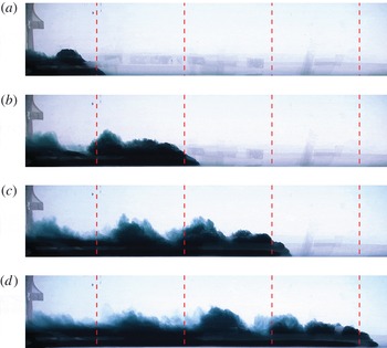
Figure 12. Photographs showing profiles of the head of the GC in Experiment 39, $\mathit{Re}_{0}=21.3\times 10^{3},x_{0}=100$
cm,
$\mathit{Re}_{0}=21.3\times 10^{3},x_{0}=100$
cm, $x_{0}/h_{0}=10.5$
. The vertical dashed lines are 20 cm apart and the times since release are 1, 2, 3 and 4 s.
$x_{0}/h_{0}=10.5$
. The vertical dashed lines are 20 cm apart and the times since release are 1, 2, 3 and 4 s.
Figure 13. Photographs showing profiles of the head of the GC in Experiment 29, $\mathit{Re}_{0}=12.9\times 10^{3}$
,
$\mathit{Re}_{0}=12.9\times 10^{3}$
, $x_{0}=6~\text{cm}$
,
$x_{0}=6~\text{cm}$
, $x_{0}/h_{0}=0.8$
. The vertical dashed lines are 20 cm apart and the times since release are 1, 2, 3 and 4 s.
$x_{0}/h_{0}=0.8$
. The vertical dashed lines are 20 cm apart and the times since release are 1, 2, 3 and 4 s.
The shape of the head of the current observed from below, shown in figure 14, is in quite good agreement with similar experiments in triangular channels; Monaghan et al. (Reference Monaghan, Mériaux, Huppert and Monaghan2009b ), also recorded a rounded shape of the head with lobes and clefts. This is expected since the shape of the head is influenced by the small length scales and is much less related to the macro length scales. However, the shrinkage of the current behind the head is an effect of the geometry of the tank: in a tank that does not have a flat bottom, a larger depth requires a larger width, hence the variable depth of the current near the head is observed as a variable width, unless strong lateral mixing and diffusing is present. The three-dimensional structure of the current is also evident in the wake which develops behind the head, with eddies rolling with the axis inclined with respect to the transverse direction.
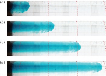
Figure 14. Photographs showing the bottom view of the head of the GC in Experiment 15 (see the online supplementary movie), $\mathit{Re}_{0}=4.1\times 10^{3}$
,
$\mathit{Re}_{0}=4.1\times 10^{3}$
, $x_{0}=100$
cm. The dashed curves are 20 cm apart and the times since release are 1.6, 3.2, 4.8 and 6.4 s.
$x_{0}=100$
cm. The dashed curves are 20 cm apart and the times since release are 1.6, 3.2, 4.8 and 6.4 s.
Figure 15. The distance of propagation of the currents measured from the gate. The solid line represents the slumping phase with $x_{N}\propto t$
, the dotted line is the inertial-buoyancy phase with
$x_{N}\propto t$
, the dotted line is the inertial-buoyancy phase with $x_{N}\propto t^{3/4}$
and the dashed line is the viscous-buoyancy phase with
$x_{N}\propto t^{3/4}$
and the dashed line is the viscous-buoyancy phase with $x_{N}\propto t^{1/4}$
.
$x_{N}\propto t^{1/4}$
.
For quantitative analysis purposes, the initial $\mathit{Re}_{0}$
(
$\mathit{Re}_{0}$
( ${>}3800$
) and the length of the channel downstream were high enough to guarantee that all of the phases of propagation predicted by the theory were reproduced. In the first phase (slumping) of the inertial-buoyancy regime, the GC front propagates at a constant speed
${>}3800$
) and the length of the channel downstream were high enough to guarantee that all of the phases of propagation predicted by the theory were reproduced. In the first phase (slumping) of the inertial-buoyancy regime, the GC front propagates at a constant speed $u_{N}$
. Then a (quite long) transition follows to the stage of inertial self-similar propagation with
$u_{N}$
. Then a (quite long) transition follows to the stage of inertial self-similar propagation with $x_{N}\propto t^{3/4}$
. Finally, the current enters the buoyancy-viscous regime where
$x_{N}\propto t^{3/4}$
. Finally, the current enters the buoyancy-viscous regime where $x_{N}\propto t^{1/4}$
(Takagi & Huppert Reference Takagi and Huppert2007). Figure 15 shows the dimensionless data pooled together for all of the experiments in a log–log plot (one experimental point out of ten is drawn for a clear visualization), together with the theoretical trends. Inspection of figure 15 clearly demonstrates a gradual, continuous transition from the slumping to the viscous phase.
$x_{N}\propto t^{1/4}$
(Takagi & Huppert Reference Takagi and Huppert2007). Figure 15 shows the dimensionless data pooled together for all of the experiments in a log–log plot (one experimental point out of ten is drawn for a clear visualization), together with the theoretical trends. Inspection of figure 15 clearly demonstrates a gradual, continuous transition from the slumping to the viscous phase.
The speed of the GC front, computed via finite differences, is depicted in figure 16; the symbols are again diluted for a better visualization. An almost constant speed is observed for all experiments in the first stage, with fluctuations that can be attributed to imperfect gate movement, random modulation of the current due to turbulence, and lobe and cleft instabilities. After the first stage, the speed of the current progressively decays.
Figure 16. The experimental speed of the GC front versus distance of propagation.
Figure 17. The experimental speed of the GC front during the slumping phase. The filled symbols refer to experiments with long lock ( $x_{0}=100~\text{cm}$
), the open symbols refer to experiments with short lock (
$x_{0}=100~\text{cm}$
), the open symbols refer to experiments with short lock ( $x_{0}=6{-}15~\text{cm}$
). The three curves are the theoretical solution. The error bars indicate one standard deviation.
$x_{0}=6{-}15~\text{cm}$
). The three curves are the theoretical solution. The error bars indicate one standard deviation.
The speed in the slumping phase is shown in figure 17 as a function of $H$
, which compares experiments (symbols) and theory (curves). The theory always overpredicts the experimental speed, with an error that depends on the experimental parameters. In an attempt to elucidate the source of the error, the correlation of the relative error with
$H$
, which compares experiments (symbols) and theory (curves). The theory always overpredicts the experimental speed, with an error that depends on the experimental parameters. In an attempt to elucidate the source of the error, the correlation of the relative error with $\mathit{Re}_{0}$
and
$\mathit{Re}_{0}$
and $\mathit{Re}_{0}(h_{0}/x_{0})$
has been analysed (see figure SM.3 in the supplementary material). The experimental data are well grouped in both cases and the error diminishes with increasing
$\mathit{Re}_{0}(h_{0}/x_{0})$
has been analysed (see figure SM.3 in the supplementary material). The experimental data are well grouped in both cases and the error diminishes with increasing $\mathit{Re}_{0}$
or
$\mathit{Re}_{0}$
or $\mathit{Re}_{0}(h_{0}/x_{0})$
, even though the former correlation seems sharper. Furthermore, assuming that the error decays as
$\mathit{Re}_{0}(h_{0}/x_{0})$
, even though the former correlation seems sharper. Furthermore, assuming that the error decays as $\log [\mathit{Re}_{0}^{a}\,(h_{0}/x_{0})^{b}]$
, a best-fit procedure yields
$\log [\mathit{Re}_{0}^{a}\,(h_{0}/x_{0})^{b}]$
, a best-fit procedure yields $a\approx 2$
and
$a\approx 2$
and $b\approx 1$
; hence, the error can be expressed as
$b\approx 1$
; hence, the error can be expressed as $\propto \log [\mathit{Re}_{0}^{2}\,(h_{0}/x_{0})]$
. The conclusion is that the SW
$\propto \log [\mathit{Re}_{0}^{2}\,(h_{0}/x_{0})]$
. The conclusion is that the SW $u_{N}$
predictions are a fair approximation (from above) for
$u_{N}$
predictions are a fair approximation (from above) for $\mathit{Re}_{0}\gtrapprox 5\times 10^{4}$
and
$\mathit{Re}_{0}\gtrapprox 5\times 10^{4}$
and $\mathit{Re}_{0}(h_{0}/x_{0})\gtrapprox 2\times 10^{4}$
; otherwise, a speed reduction larger than 20 % is expected.
$\mathit{Re}_{0}(h_{0}/x_{0})\gtrapprox 2\times 10^{4}$
; otherwise, a speed reduction larger than 20 % is expected.
For the detection of the various phases of motion, we proceed as follows. Assuming that $x_{N}=Kt^{{\it\gamma}}$
, the local values of the exponent
$x_{N}=Kt^{{\it\gamma}}$
, the local values of the exponent ${\it\gamma}$
can be evaluated by observing that
${\it\gamma}$
can be evaluated by observing that ${\dot{x}}_{N}=K{\it\gamma}t^{{\it\gamma}-1}$
, hence
${\dot{x}}_{N}=K{\it\gamma}t^{{\it\gamma}-1}$
, hence ${\it\gamma}={\dot{x}}_{N}t/x_{N}$
, with
${\it\gamma}={\dot{x}}_{N}t/x_{N}$
, with ${\dot{x}}_{N}$
estimated using finite difference (the upper dot denotes time derivative). The value of
${\dot{x}}_{N}$
estimated using finite difference (the upper dot denotes time derivative). The value of $K$
is computed as
$K$
is computed as $K=x_{N}/t^{{\it\gamma}}$
. Figure 18 shows the computed values of
$K=x_{N}/t^{{\it\gamma}}$
. Figure 18 shows the computed values of ${\it\gamma}$
and
${\it\gamma}$
and $K$
for the short lock experiments. The plot for
$K$
for the short lock experiments. The plot for ${\it\gamma}$
indicates values close to unity near the gate, followed by a progressive reduction down to 0.25 in the farthest sections. The plot for the coefficient
${\it\gamma}$
indicates values close to unity near the gate, followed by a progressive reduction down to 0.25 in the farthest sections. The plot for the coefficient $K$
indicates that the space variation of the coefficient is controlled by the non-dimensional group
$K$
indicates that the space variation of the coefficient is controlled by the non-dimensional group $\mathit{Re}_{0}(h_{0}/x_{0})$
, with an asymptotic independence at large values of
$\mathit{Re}_{0}(h_{0}/x_{0})$
, with an asymptotic independence at large values of $\mathit{Re}_{0}(h_{0}/x_{0})$
. The line of Experiment 33 deviates significantly from the slumping pattern displayed by the other records in figure 18(a). We have no explanation for this strange behaviour; we speculate there was some mechanical or electrical problem with the gate-opening device.
$\mathit{Re}_{0}(h_{0}/x_{0})$
. The line of Experiment 33 deviates significantly from the slumping pattern displayed by the other records in figure 18(a). We have no explanation for this strange behaviour; we speculate there was some mechanical or electrical problem with the gate-opening device.
Figure 18. The experimental exponent ${\it\gamma}$
(a) and coefficient
${\it\gamma}$
(a) and coefficient $K$
(b) for an advancement of the GC front of the form
$K$
(b) for an advancement of the GC front of the form $x_{N}=Kt^{{\it\gamma}}$
. In (a) the dash-dot line corresponds to
$x_{N}=Kt^{{\it\gamma}}$
. In (a) the dash-dot line corresponds to ${\it\gamma}=1$
, typical of the slumping stage, the dotted line corresponds to
${\it\gamma}=1$
, typical of the slumping stage, the dotted line corresponds to ${\it\gamma}=3/4$
, typical of the propagation in the self-similar inertial-buoyancy regime, while the dashed line corresponds to
${\it\gamma}=3/4$
, typical of the propagation in the self-similar inertial-buoyancy regime, while the dashed line corresponds to ${\it\gamma}=1/4$
, typical of the propagation in the buoyancy-viscous regime. Experiments with short lock,
${\it\gamma}=1/4$
, typical of the propagation in the buoyancy-viscous regime. Experiments with short lock, $x_{0}=6{-}15~\text{cm}$
.
$x_{0}=6{-}15~\text{cm}$
.
We have rechecked the assumption that the Boussinesq approximation errors are small. First, we found that the scaled experimental results for different density contrasts collapse within the estimated $0.5(1-R)$
error, which is also in the range of the experimental error. Second, using the SW theoretical model, we compared typical predictions for
$0.5(1-R)$
error, which is also in the range of the experimental error. Second, using the SW theoretical model, we compared typical predictions for $R=0.9$
and
$R=0.9$
and $R=1$
. The theoretical speeds
$R=1$
. The theoretical speeds $u_{N},V_{f}$
in the first case are slightly larger than in the second, but the differences are at most 4 %. This is, again, in agreement with the estimate that the relative error of the Boussinesq simplification is approximately
$u_{N},V_{f}$
in the first case are slightly larger than in the second, but the differences are at most 4 %. This is, again, in agreement with the estimate that the relative error of the Boussinesq simplification is approximately $0.5(1-R)$
. Evidently, the investigation of non-Boussinesq effects requires significantly larger density contrasts than the 10.6 % of our experiments.
$0.5(1-R)$
. Evidently, the investigation of non-Boussinesq effects requires significantly larger density contrasts than the 10.6 % of our experiments.
Figure 19. Transition to viscous regime as a function of $\mathit{Re}_{0}(h_{0}/x_{0})$
. The bold line represents the theoretical estimate
$\mathit{Re}_{0}(h_{0}/x_{0})$
. The bold line represents the theoretical estimate $x_{V}=0.5[\mathit{Re}_{0}(h_{0}/x_{0})]^{3/8}$
, the dashed lines are the best-fit curves of equation
$x_{V}=0.5[\mathit{Re}_{0}(h_{0}/x_{0})]^{3/8}$
, the dashed lines are the best-fit curves of equation $x_{V}=0.43[\mathit{Re}_{0}(h_{0}/x_{0})]^{0.47}$
,
$x_{V}=0.43[\mathit{Re}_{0}(h_{0}/x_{0})]^{0.47}$
, $x_{V}=1.20[\mathit{Re}_{0}(h_{0}/x_{0})]^{0.28}$
and
$x_{V}=1.20[\mathit{Re}_{0}(h_{0}/x_{0})]^{0.28}$
and $x_{V}=1.20[\mathit{Re}_{0}(h_{0}/x_{0})]^{0.27}$
calculated assuming an exponent
$x_{V}=1.20[\mathit{Re}_{0}(h_{0}/x_{0})]^{0.27}$
calculated assuming an exponent ${\it\gamma}=0.5$
(circles),
${\it\gamma}=0.5$
(circles), ${\it\gamma}=0.7$
(squares) and
${\it\gamma}=0.7$
(squares) and ${\it\gamma}=0.75$
(crosses), respectively.
${\it\gamma}=0.75$
(crosses), respectively.
Even though a plateau of the exponent ${\it\gamma}$
is observed in figure 18 for a few lock-lengths, which is a strong indication of the existence of the constant-speed slumping phase, the scatter of the data prevents an accurate evaluation of the extent of the slumping phase
${\it\gamma}$
is observed in figure 18 for a few lock-lengths, which is a strong indication of the existence of the constant-speed slumping phase, the scatter of the data prevents an accurate evaluation of the extent of the slumping phase $x_{s}$
. The typical values are 4–7, and the maximum is approximately 10; the larger values correspond in general to smaller
$x_{s}$
. The typical values are 4–7, and the maximum is approximately 10; the larger values correspond in general to smaller $H$
. This is consistent with theoretical estimates based on the speed of the bores/waves in the lock and after reflection.
$H$
. This is consistent with theoretical estimates based on the speed of the bores/waves in the lock and after reflection.
The transition to the viscous regime is amenable to a sharper analysis. Figure 19 shows the distance of transition according to the theoretical estimation (equation (2.3)) and to the experimental data. The latter is evaluated assuming that the transition is marked by a threshold value of the exponent ${\it\gamma}$
taken to be equal to 0.5, 0.7 or 0.75. Changing the threshold from 0.7 to 0.75 reduces
${\it\gamma}$
taken to be equal to 0.5, 0.7 or 0.75. Changing the threshold from 0.7 to 0.75 reduces $x_{V}$
but does not modify significantly the exponent of
$x_{V}$
but does not modify significantly the exponent of $\mathit{Re}(h_{0}/x_{0})$
, whose measured value is 0.275, while the theory overpredicts
$\mathit{Re}(h_{0}/x_{0})$
, whose measured value is 0.275, while the theory overpredicts $3/8=0.375$
. The threshold 0.5 indicates a transition length almost twice the theoretical one. The discrepancy between theory and experiments can be attributed to: first, the theoretical estimation is based on asymptotic formulae valid for long propagations, that are applied here at a finite distance from the gate; this introduces an error, that is not uniform in the different experiments; second, the experimental evaluation of
$3/8=0.375$
. The threshold 0.5 indicates a transition length almost twice the theoretical one. The discrepancy between theory and experiments can be attributed to: first, the theoretical estimation is based on asymptotic formulae valid for long propagations, that are applied here at a finite distance from the gate; this introduces an error, that is not uniform in the different experiments; second, the experimental evaluation of $x_{V}$
is also prone to uncertainties (mainly because the transition point lacks a rigorous definition in terms of a sharp measurable property). There is evidence that the trend of
$x_{V}$
is also prone to uncertainties (mainly because the transition point lacks a rigorous definition in terms of a sharp measurable property). There is evidence that the trend of $x_{V}$
is correctly predicted, as
$x_{V}$
is correctly predicted, as $x_{V}$
indeed increases with a power of
$x_{V}$
indeed increases with a power of $\mathit{Re}_{0}(h_{0}/x_{0})$
. However, the theory apparently overpredicts it (in our experiments by approximately 33 %). The present experimental power 0.275 is actually close to the value
$\mathit{Re}_{0}(h_{0}/x_{0})$
. However, the theory apparently overpredicts it (in our experiments by approximately 33 %). The present experimental power 0.275 is actually close to the value $2/7=0.286$
predicted for a flat bottom. In our opinion, this is just coincidence because there are really significant differences between the viscous flows on flat and curved bottoms (Takagi & Huppert Reference Takagi and Huppert2007). More experiments are necessary for a clarification of this issue.
$2/7=0.286$
predicted for a flat bottom. In our opinion, this is just coincidence because there are really significant differences between the viscous flows on flat and curved bottoms (Takagi & Huppert Reference Takagi and Huppert2007). More experiments are necessary for a clarification of this issue.
5. Conclusions
In this paper we have analysed in detail the propagation of a high-Reynolds-number GC released from a lock (of length $x_{0}$
and height
$x_{0}$
and height $h_{0}$
) in a channel of circular/semicircular cross-section, in the Boussinesq regime. We have conducted two series of experiments in which we have measured the speed and amplitude of the waves or bores in the lock (29 experiments), and the time-dependent propagation of the current downstream (10 experiments). The denser fluid was a saline solution, released from a lock by rapidly removing a vertical gate in a horizontal channel with circular cross-section. The ambient fluid was fresh water. The addition of aniline dye to the denser fluid enabled the recording of its motion with photo and video cameras. The novelties of our work are: (i) the shape of the channel; (ii) the systematic analysis of the effects of the ratio
$h_{0}$
) in a channel of circular/semicircular cross-section, in the Boussinesq regime. We have conducted two series of experiments in which we have measured the speed and amplitude of the waves or bores in the lock (29 experiments), and the time-dependent propagation of the current downstream (10 experiments). The denser fluid was a saline solution, released from a lock by rapidly removing a vertical gate in a horizontal channel with circular cross-section. The ambient fluid was fresh water. The addition of aniline dye to the denser fluid enabled the recording of its motion with photo and video cameras. The novelties of our work are: (i) the shape of the channel; (ii) the systematic analysis of the effects of the ratio $H=H^{\ast }/h_{0}$
on the speed of propagation of the current downstream; (iii) the experimental validation of the dynamics of the flow in the lock as described by a two-layer SW model (left-moving jump/rarefaction wave into the stagnant fluid, and the reflection); (iv) the theoretical and experimental determination of the distance
$H=H^{\ast }/h_{0}$
on the speed of propagation of the current downstream; (iii) the experimental validation of the dynamics of the flow in the lock as described by a two-layer SW model (left-moving jump/rarefaction wave into the stagnant fluid, and the reflection); (iv) the theoretical and experimental determination of the distance $x_{V}$
where the transition to viscous regime occurs. We used a channel of 615 cm length which allowed a propagation of up to 100 lock lengths.
$x_{V}$
where the transition to viscous regime occurs. We used a channel of 615 cm length which allowed a propagation of up to 100 lock lengths.
The observed flow in the lock is close to the theoretical prediction of SW (inviscid flow) model. The speed of the bore/rarefaction wave is overestimated by the model, but the discrepancy decreases as the Reynolds numbers $\mathit{Re}_{0}$
or
$\mathit{Re}_{0}$
or $\mathit{Re}_{0}(h_{0}/x_{0})$
increase, and is within the range of the experimental error for
$\mathit{Re}_{0}(h_{0}/x_{0})$
increase, and is within the range of the experimental error for $\mathit{Re}_{0}\gtrapprox 3\times 10^{4}$
or
$\mathit{Re}_{0}\gtrapprox 3\times 10^{4}$
or $\mathit{Re}_{0}(h_{0}/x_{0})\gtrapprox 5\times 10^{3}$
.
$\mathit{Re}_{0}(h_{0}/x_{0})\gtrapprox 5\times 10^{3}$
.
There are, however, some theoretical predictions that could not be corroborated in our experiments. The predicted stationary jump at $x=0$
in the full-circle full-depth
$x=0$
in the full-circle full-depth ${\it\beta}=2,H=1$
geometry, see figure 2(d), could not be observed because of a built-in obstacle. Moreover, in our experiments it was not possible to distinguish between flows of type 2 and type 3; it is well known that in practice, under the influence of the no-slip condition, the GC front is not a sharp vertical jump, but rather a curved head. Therefore, Navier–Stokes numerical simulation with a free-slip bottom condition must be used for the verification of the types 2–3 differences predicted by the SW theory.
${\it\beta}=2,H=1$
geometry, see figure 2(d), could not be observed because of a built-in obstacle. Moreover, in our experiments it was not possible to distinguish between flows of type 2 and type 3; it is well known that in practice, under the influence of the no-slip condition, the GC front is not a sharp vertical jump, but rather a curved head. Therefore, Navier–Stokes numerical simulation with a free-slip bottom condition must be used for the verification of the types 2–3 differences predicted by the SW theory.
The parameter ${\it\beta}=H^{\ast }/r^{\ast }$
(height of ambient to radius,
${\it\beta}=H^{\ast }/r^{\ast }$
(height of ambient to radius, ${\leqslant}2$
) has a rather small influence on the behaviour of the current (except for
${\leqslant}2$
) has a rather small influence on the behaviour of the current (except for ${\it\beta}$
close to 2). This is in agreement with theoretical predictions. The measured speed of the current downstream shows that the high-Reynolds-number (
${\it\beta}$
close to 2). This is in agreement with theoretical predictions. The measured speed of the current downstream shows that the high-Reynolds-number ( $\mathit{Re}_{0}\gg 1$
) buoyancy-inertial current eventually transits to the viscous regime investigated by Takagi & Huppert (Reference Takagi and Huppert2007). The distance
$\mathit{Re}_{0}\gg 1$
) buoyancy-inertial current eventually transits to the viscous regime investigated by Takagi & Huppert (Reference Takagi and Huppert2007). The distance $x_{V}$
where viscosity becomes dominant increases like
$x_{V}$
where viscosity becomes dominant increases like $[\mathit{Re}_{0}(h_{0}/x_{0})]^{{\it\alpha}}$
as predicted by the theoretical estimate developed in this paper, but the experimental
$[\mathit{Re}_{0}(h_{0}/x_{0})]^{{\it\alpha}}$
as predicted by the theoretical estimate developed in this paper, but the experimental ${\it\alpha}\approx 0.27$
is smaller than the predicted 0.375. The discrepancy is attributed mostly to the fact that the
${\it\alpha}\approx 0.27$
is smaller than the predicted 0.375. The discrepancy is attributed mostly to the fact that the $x_{V}$
estimate assumes fully developed ideal self-similar flows, while in practice the inertial flow is contaminated by the no-slip condition from an early stage. The Boussinesq approximation is acceptable for the tested cases, and hence the present results can be used with confidence also for a ‘light’ (top) current by redefining
$x_{V}$
estimate assumes fully developed ideal self-similar flows, while in practice the inertial flow is contaminated by the no-slip condition from an early stage. The Boussinesq approximation is acceptable for the tested cases, and hence the present results can be used with confidence also for a ‘light’ (top) current by redefining $g^{\prime }$
as
$g^{\prime }$
as $(1-R)g$
, and measuring
$(1-R)g$
, and measuring $z$
from the upper side.
$z$
from the upper side.
Our work elucidates similarities and differences between the propagation of the current in the circle/semicircle cross-section and in the classical rectangular case. The same main stages of propagation occur: first slumping with constant $u_{N}$
, then self-similar with decaying
$u_{N}$
, then self-similar with decaying $u_{N}\sim t^{{\it\gamma}-1}$
, and eventually transition to the viscous regime at
$u_{N}\sim t^{{\it\gamma}-1}$
, and eventually transition to the viscous regime at $x_{V}\sim [\mathit{Re}_{0}(h_{0}/x_{0})]^{{\it\alpha}}$
. The main governing parameters are the same, and the trends of influence are consistent: as
$x_{V}\sim [\mathit{Re}_{0}(h_{0}/x_{0})]^{{\it\alpha}}$
. The main governing parameters are the same, and the trends of influence are consistent: as $H$
increases, the speed increases, and the slumping distance decreases; also,
$H$
increases, the speed increases, and the slumping distance decreases; also, $x_{V}\propto [\mathit{Re}_{0}(h_{0}/x_{0})]^{{\it\alpha}}$
. The differences are mostly on the quantitative side: here the
$x_{V}\propto [\mathit{Re}_{0}(h_{0}/x_{0})]^{{\it\alpha}}$
. The differences are mostly on the quantitative side: here the $u_{N}$
is larger, the transition between stages is over a longer time/length interval,
$u_{N}$
is larger, the transition between stages is over a longer time/length interval, ${\it\gamma}=3/4$
(instead of
${\it\gamma}=3/4$
(instead of $2/3$
) and
$2/3$
) and ${\it\alpha}=3/8$
(instead of
${\it\alpha}=3/8$
(instead of $2/7$
, theoretically; in our experiment the larger value of
$2/7$
, theoretically; in our experiment the larger value of ${\it\alpha}$
was not confirmed). The input parameter
${\it\alpha}$
was not confirmed). The input parameter ${\it\beta}$
has no counterpart in the classical flat-bottom channel; however, as mentioned above, this parameter is quite insignificant.
${\it\beta}$
has no counterpart in the classical flat-bottom channel; however, as mentioned above, this parameter is quite insignificant.
In particular, we found that the initial slumping speed displays the predicted dependency on the height ratio $H$
, but the values were by typically 15 % below the SW model predictions. This could be expected: the GC front is affected by the viscous no-slip condition, which is not incorporated in the model. Again, the slumping propagation in a semicircle is faster than in a rectangle. For example, for
$H$
, but the values were by typically 15 % below the SW model predictions. This could be expected: the GC front is affected by the viscous no-slip condition, which is not incorporated in the model. Again, the slumping propagation in a semicircle is faster than in a rectangle. For example, for $H=1$
: in a circle
$H=1$
: in a circle ${\it\beta}=2$
the measured slumping speed is
${\it\beta}=2$
the measured slumping speed is $u_{N}=0.54$
, while in a rectangle (Lowe, Rottman & Linden Reference Lowe, Rottman and Linden2005) the measured
$u_{N}=0.54$
, while in a rectangle (Lowe, Rottman & Linden Reference Lowe, Rottman and Linden2005) the measured $u_{N}=0.42$
(the theoretical predictions are 0.57 and 0.54, respectively). The reason for the larger speed is readily attributed to geometrical influence: for a given
$u_{N}=0.42$
(the theoretical predictions are 0.57 and 0.54, respectively). The reason for the larger speed is readily attributed to geometrical influence: for a given $H$
, the area ratio of ambient to current fluid is larger in the typical circular channel, and thus the propagating current encounters a smaller return-flow effect. In other words, the current in the circle, for a given
$H$
, the area ratio of ambient to current fluid is larger in the typical circular channel, and thus the propagating current encounters a smaller return-flow effect. In other words, the current in the circle, for a given $H$
, propagates like one in a rectangle of larger
$H$
, propagates like one in a rectangle of larger $H$
. The first theoretical indication to this result is the fact that
$H$
. The first theoretical indication to this result is the fact that $Fr(a)$
is larger for a circle, where
$Fr(a)$
is larger for a circle, where $a=h_{N}/H$
(see figure SM.1 in the supplementary material).
$a=h_{N}/H$
(see figure SM.1 in the supplementary material).
The fact that the experiments provide fair support to the theoretical predictions in this system is, in our opinion, of some general importance to the methodology of understanding and modeling of GC. The investigation of non-rectangular cross-section currents is a relatively new topic, and it is not clear a priori if and how well this problem can be connected to the classical flat-bottom-current methodology and insights.
We found that the agreements between the theoretical predictions and the experimental observations in the new problem are essentially the same as in the classical problem. We recall that the measured speed of propagation in the slumping stage in a rectangular channel, for which a large body of data is available (see Rottman & Simpson Reference Rottman and Simpson1983; Shin, Dalziel & Linden Reference Shin, Dalziel and Linden2004; Lowe et al. Reference Lowe, Rottman and Linden2005), is typically 20 % below the rigorous SW prediction. In the present case, the measured values are typically 15 % below the predictions. This is an encouraging outcome, with some practical benefit. Unlike the rectangular case which can be simulated by 2D codes, the current in a circular/semicircular cross-section channel must be simulated by time and memory consuming 3D codes. The need for the simplified model is thus enhanced, and the information that the predictions agree with physical observations provides confidence.
The experience with classical-rectangular GC indicates that it is possible to improve the agreement between the theoretical speed predictions and measurements by using instead of the theoretical $\mathit{Fr}$
of Benjamin (Reference Benjamin1968) an empirically adjusted
$\mathit{Fr}$
of Benjamin (Reference Benjamin1968) an empirically adjusted $\mathit{Fr}$
(e.g. the formula of Huppert & Simpson (Reference Huppert and Simpson1980)). However, such a formula is unavailable for the circle cross-section. Whether and how such improvements work in the present problem is a topic of further research.
$\mathit{Fr}$
(e.g. the formula of Huppert & Simpson (Reference Huppert and Simpson1980)). However, such a formula is unavailable for the circle cross-section. Whether and how such improvements work in the present problem is a topic of further research.
Our experiments suggest that a better agreement with theory could be expected for significantly larger $\mathit{Re}_{0}(h_{0}/x_{0})$
, while keeping
$\mathit{Re}_{0}(h_{0}/x_{0})$
, while keeping $h_{0}/x_{0}$
small. This would produce both a larger
$h_{0}/x_{0}$
small. This would produce both a larger $u_{N}$
and a longer
$u_{N}$
and a longer $x_{V}$
; the latter will allow a sharper self-similar inertia-buoyancy stage of propagation. Unfortunately, data acquisition in this parameter range requires a significant, and very expensive, scale-up of the experimental apparatus in height, width and length. This is beyond the capability of the typical academic-institute fluid-mechanics laboratory. The more feasible alternative is to attempt ‘numerical experiments’; an advantage of this option is that free-slip boundary condition can be used for a sharper assessment of the
$x_{V}$
; the latter will allow a sharper self-similar inertia-buoyancy stage of propagation. Unfortunately, data acquisition in this parameter range requires a significant, and very expensive, scale-up of the experimental apparatus in height, width and length. This is beyond the capability of the typical academic-institute fluid-mechanics laboratory. The more feasible alternative is to attempt ‘numerical experiments’; an advantage of this option is that free-slip boundary condition can be used for a sharper assessment of the $\mathit{Fr}$
condition. Although neither cheap nor straightforward, such simulations are expected to be more advantageous than large-scale laboratory experiments. The numerical ‘state of the art’ seems ripe for such simulation (Constantinescu Reference Constantinescu2014; Nasr-Azadani & Meiburg Reference Nasr-Azadani and Meiburg2014) and we hope that the present investigation will provide both motivation and reference data for such a numerical study in the near future.
$\mathit{Fr}$
condition. Although neither cheap nor straightforward, such simulations are expected to be more advantageous than large-scale laboratory experiments. The numerical ‘state of the art’ seems ripe for such simulation (Constantinescu Reference Constantinescu2014; Nasr-Azadani & Meiburg Reference Nasr-Azadani and Meiburg2014) and we hope that the present investigation will provide both motivation and reference data for such a numerical study in the near future.
Finally, we recall that a current in full-circle full-depth channel ${\it\beta}=2,H=1$
was discussed briefly in Benjamin’s (Reference Benjamin1968) classical paper. The solution for the steady-state half-infinite current was presented only for the non-dissipative propagation. The speed is, in our notation,
${\it\beta}=2,H=1$
was discussed briefly in Benjamin’s (Reference Benjamin1968) classical paper. The solution for the steady-state half-infinite current was presented only for the non-dissipative propagation. The speed is, in our notation, $u_{N}=0.542$
. It is remarkable that our experimental result for the slumping speed in the
$u_{N}=0.542$
. It is remarkable that our experimental result for the slumping speed in the ${\it\beta}=2,H=1$
channel is 0.54. The SW dam-break solution, which allows dissipation, produces the slightly larger
${\it\beta}=2,H=1$
channel is 0.54. The SW dam-break solution, which allows dissipation, produces the slightly larger $u_{N}=0.57$
. The apparently perfect agreement with the experiment does not demonstrate that Benjamin’s theoretical result is the ‘better’ one. Since there certainly is a viscous no-slip speed reduction in the real current, the ‘correct’ inviscid
$u_{N}=0.57$
. The apparently perfect agreement with the experiment does not demonstrate that Benjamin’s theoretical result is the ‘better’ one. Since there certainly is a viscous no-slip speed reduction in the real current, the ‘correct’ inviscid $u_{N}$
result must be larger than the measured speed. The clarification of this issue must be left, again, to Navier–Stokes simulation in which a free-slip boundary condition can be tested.
$u_{N}$
result must be larger than the measured speed. The clarification of this issue must be left, again, to Navier–Stokes simulation in which a free-slip boundary condition can be tested.
Supplementary material
Some calculations on the theoretical model, two figures related to the reflected bores and the GC front speed, two videos of the experiments with superscript ‘ $a$
’ in table 2 and the experimental time series of the GC front position for the 10 experiments listed in the same table, in .txt format.
$a$
’ in table 2 and the experimental time series of the GC front position for the 10 experiments listed in the same table, in .txt format.
Supplementary material is available at http://dx.doi.org/10.1017/jfm.2014.701.
Appendix A. Theoretical estimate of $x_{V}$

We use dimensionless variables as defined in § 2, unless stated otherwise.
Let $x_{V}$
be the length where the current changes regime from inertial to viscous. Suppose that in both regimes a similarity solution is relevant,
$x_{V}$
be the length where the current changes regime from inertial to viscous. Suppose that in both regimes a similarity solution is relevant,
 $$\begin{eqnarray}x_{N}(t)=K_{j}t^{{\it\gamma}_{j}}\end{eqnarray}$$
where $j=I$
for inertial and
$j=I$
for inertial and $j=V$
for viscous and the values of
$j=V$
for viscous and the values of $K_{j}$
and
$K_{j}$
and ${\it\gamma}_{j}$
are known.
${\it\gamma}_{j}$
are known.
The speed of propagation is
 $$\begin{eqnarray}u_{N}={\dot{x}}_{N}={\it\gamma}_{j}K_{j}t^{{\it\gamma}_{j}-1}.\end{eqnarray}$$
Note that $t=(x_{N}/K)^{1/{\it\gamma}}$
. Hence, equation (A 2) can be rewritten as
$t=(x_{N}/K)^{1/{\it\gamma}}$
. Hence, equation (A 2) can be rewritten as
 $$\begin{eqnarray}u_{N}={\it\gamma}_{j}K_{j}^{1/{\it\gamma}_{j}}x_{N}^{1-1/{\it\gamma}_{j}}.\end{eqnarray}$$
We assume that the transition from inertial to viscous regimes is between two self-similar forms. We argue that the transition is smooth and, hence, at this occurrence, both regimes display the same speed of propagation. We therefore write, for the transition
 $$\begin{eqnarray}{\it\gamma}_{I}K_{I}^{1/{\it\gamma}_{I}}x_{N}^{1-1/{\it\gamma}_{I}}={\it\gamma}_{V}K_{V}^{1/{\it\gamma}_{V}}x_{N}^{1-1/{\it\gamma}_{V}}.\end{eqnarray}$$
The value of $x_{N}$
which satisfies this equation is the transition
$x_{N}$
which satisfies this equation is the transition $x_{V}$
. We obtain
$x_{V}$
. We obtain
 $$\begin{eqnarray}x_{V}=\left[\frac{{\it\gamma}_{I}K_{I}^{1/{\it\gamma}_{I}}}{{\it\gamma}_{V}K_{V}^{1/{\it\gamma}_{V}}}\right]^{q};\quad q=\frac{{\it\gamma}_{I}{\it\gamma}_{V}}{{\it\gamma}_{V}-{\it\gamma}_{I}}.\end{eqnarray}$$
For the circle we note the following.
(i) The viscous regime was solved by Takagi & Huppert (Reference Takagi and Huppert2007, (2.19b)). This provides ${\it\gamma}_{V}=1/4$
and, after scaling, also
${\it\gamma}_{V}=1/4$
and, after scaling, also
 $$\begin{eqnarray}K_{V}=[P\,\mathit{Re}_{0}(h_{0}/x_{0})]^{{\it\gamma}_{V}}\end{eqnarray}$$
where
 $$\begin{eqnarray}P=2^{10}/(105{\rm\pi}^{2})\approx 0.99.\end{eqnarray}$$
In this evaluation we used the approximation $V^{2}/r=32h_{0}^{3}x_{0}^{2}/9$
where
$V^{2}/r=32h_{0}^{3}x_{0}^{2}/9$
where $V$
and
$V$
and $r$
are the dimensional volume of the current and radius of the channel (valid for
$r$
are the dimensional volume of the current and radius of the channel (valid for $r\geqslant h_{0}$
).
$r\geqslant h_{0}$
).
(ii) For a thin current (compared to the radius of the channel) the inertial solution for the circle is well approximated by the power-law width function $bz^{1/2}$
. For the latter case, Zemach & Ungarish (Reference Zemach and Ungarish2013) derived the self-similar solution and provide
$bz^{1/2}$
. For the latter case, Zemach & Ungarish (Reference Zemach and Ungarish2013) derived the self-similar solution and provide ${\it\gamma}_{I}=3/4,K_{I}=1.765$
. Substitution into (A 5) and some algebra yields
${\it\gamma}_{I}=3/4,K_{I}=1.765$
. Substitution into (A 5) and some algebra yields
 $$\begin{eqnarray}x_{V}=0.50\left(\mathit{Re}_{0}h_{0}/x_{0}\right)^{3/8}.\end{eqnarray}$$
We recall that for a standard rectangular cross-section the estimated transition from inertial to viscous regime is given by $x_{V}=C_{1}[\mathit{Re}_{0}(h_{0}/x_{0})]^{2/7}$
, where
$x_{V}=C_{1}[\mathit{Re}_{0}(h_{0}/x_{0})]^{2/7}$
, where $C_{1}$
is a constant of order unity (see Ungarish (Reference Ungarish2013, §2.7), and the references therein). It is interesting to note that in both cases the relevant Reynolds number is actually
$C_{1}$
is a constant of order unity (see Ungarish (Reference Ungarish2013, §2.7), and the references therein). It is interesting to note that in both cases the relevant Reynolds number is actually $\mathit{Re}_{0}(h_{0}/x_{0})$
.
$\mathit{Re}_{0}(h_{0}/x_{0})$
.
It is surprising that, for a given $\mathit{Re}_{0}(h_{0}/x_{0})$
the flat-bottom current becomes viscous at a shorter propagation than the counterpart in the semicircle. Upon propagation, the height of the current decreases faster in the first case, and therefore the speed and inertia effects decay faster, in favour of the viscous hindrance.
$\mathit{Re}_{0}(h_{0}/x_{0})$
the flat-bottom current becomes viscous at a shorter propagation than the counterpart in the semicircle. Upon propagation, the height of the current decreases faster in the first case, and therefore the speed and inertia effects decay faster, in favour of the viscous hindrance.


