


1. Introduction
A solid particle executing small-amplitude oscillations in a viscous fluid intrinsically generates a steady streaming flow. These flows have been studied extensively using both theoretical and experimental approaches with canonical problems including the rectilinear oscillation of spheres (Riley Reference Riley1966; Dohara Reference Dohara1982; Chang & Maxey Reference Chang and Maxey1994; Li et al. Reference Li, Collis, Brumley, Schneiders and Sader2023) and cylinders (Andres & Ingard Reference Andres and Ingard1953; Bertelsen, Svardal & Tjøtta Reference Bertelsen, Svardal and Tjøtta1973; Chong et al. Reference Chong, Kelly, Smith and Eldredge2013). Asymmetry in the particle or its motion (e.g. through shape or density) inevitably leads to an asymmetric streaming flow, which in turn can apply a steady net force on the particle, generating locomotion. This phenomenon, which is often called ‘acoustic propulsion’, was originally identified by Nadal & Lauga (Reference Nadal and Lauga2014) who studied the translatory oscillations of nearly spherical particles in the low-frequency limit, i.e. the particles do not perform rotational oscillations. Collis, Chakraborty & Sader (Reference Collis, Chakraborty and Sader2017, Reference Collis, Chakraborty and Sader2022) subsequently studied the motion of a general asymmetric particle at arbitrary frequency, and showed that the propulsion direction reverses at a critical frequency. This finding was confirmed by Nadal & Michelin (Reference Nadal and Michelin2020) and Derr et al. (Reference Derr, Dombrowski, Rycroft and Klotsa2022). Interestingly, Lippera et al. (Reference Lippera, Dauchot, Michelin and Benzaquen2019) proved that to first-order in particle non-sphericity, translational oscillations alone cannot generate propulsion; contrary to Nadal & Lauga (Reference Nadal and Lauga2014). These works establish that translational and rotational particle oscillations are both required to generate propulsion. Moreover, they show that the frequency at which propulsion reverses direction is sensitively dependent on the magnitude and phase of the two oscillatory motions. The structure of streaming flows is known to change at a critical frequency (Chang & Maxey Reference Chang and Maxey1994; Li et al. Reference Li, Collis, Brumley, Schneiders and Sader2023), indicating that this change in flow structure may somehow be connected with the change in propulsion direction. The aim of this study is to explore this connection and identify the physical mechanism giving rise to this reversal in propulsion direction. Because studies typically invoke the Lorentz reciprocal theorem to calculate the particle propulsion, an explicit calculation of the flow field, and in turn how it generates propulsion, has not been reported. We address this gap in the literature and thereby identify the physical mechanism that reverses the propulsion direction.
The steady streaming flow generated by the superposition of rectilinear and rotational motions has been investigated in several studies. Kelly (Reference Kelly1966) studied the steady streaming flow around a cylinder undergoing coupled oscillations along and perpendicular to the cylinder's longitudinal axis. Later, Panagopoulos, Psillakis & Karahalios (Reference Panagopoulos, Psillakis and Karahalios1991) and Riley (Reference Riley1991) studied the streaming flow around a cylinder undergoing simultaneous oscillations that are rectilinearly perpendicular to and rotational around its longitudinal axis. Gopinath (Reference Gopinath1994) further studied the streaming flow around a sphere undergoing simultaneous rotational and translational oscillations, both about the same axis. Kong, Penkova & Sadhal (Reference Kong, Penkova and Sadhal2017) studied a closely related problem where instead of an unbounded domain the oscillating sphere is enclosed by a larger stationary sphere. These streaming flows all exhibit an asymmetry due to the superposed motions. However, none of these works investigate whether a net force or torque arises on the solid body. It remains an open question as to how the streaming flow results in the propulsion direction reversing at a critical frequency.
Collis et al. (Reference Collis, Chakraborty and Sader2017, Reference Collis, Chakraborty and Sader2022) and Nadal & Michelin (Reference Nadal and Michelin2020) both demonstrate that acoustic propulsion can be achieved through coupled rotation and translation of a sphere. Motivated by this observation, we study a sphere executing rotational oscillations in a viscous fluid whose far field undergoes rectilinear oscillations. This models the experimental set-up of a particle trapped at a pressure node of an acoustic field, where the particle is much smaller than the acoustic wavelength. To induce both translational and rotational oscillations, an asymmetry must be present in the sphere or its forcing, e.g. through an inhomogeneous density distribution or through the addition of magnetic fields (Valdez-Garduño et al. Reference Valdez-Garduño, Leal-Estrada, Oliveros-Mata, Sandoval-Bojorquez, Soto, Wang and Garcia-Gradilla2020). The primary focus here is to elucidate the mechanism giving rise to a reversal in propulsion direction at a critical frequency, and its connection to the generated streaming flow. In § 2 we derive an analytical solution to the flow field. In § 3 we explore the mechanism responsible for propulsion, and in particular examine bifurcations in the flow field and their connection to a reversal in the net hydrodynamic force experienced by the particle. Finally, in § 4 we discuss how these results may be used in modelling suspensions of acoustically propelled particles.
2. Analytical solution for the propulsion component of the streaming flow
We consider a sphere of radius  $R$ performing rotational oscillations in an unbounded, incompressible Newtonian fluid. This fluid performs independent oscillations in its far field at an identical frequency with a velocity field of $U_{\infty }\exp ({-\mathrm {i}\omega t})\boldsymbol {i}$ where $\mathrm {i}$ is the imaginary unit, $\omega$ is the oscillation frequency, $t$ is time and $\boldsymbol {i}$ is the Cartesian basis vector in the $x$-direction. The angular velocity of the sphere is $\varOmega \exp ({-\mathrm {i}(\omega t-\zeta )})\boldsymbol {j}$ where $\boldsymbol {j}$ is the Cartesian basis vector in the $y$-direction and $\zeta$ is the phase difference between the two oscillations; see figure 1(a). Note that $U_\infty$, $\varOmega$, $\zeta$ and $\omega$ are all positive and real constants with the true (as measured) quantities being given by the real parts of all expressions. Scaling the spatial variables by $R$, time by $1/\omega$, velocity by $U_\infty$ and pressure by $\mu U_\infty /R$ (hence force by $\mu U_\infty R$), where $\mu$ is the fluid's shear viscosity, gives the dimensionless Navier–Stokes equations
 \begin{equation} \boldsymbol{\nabla}\boldsymbol{\cdot} \boldsymbol{u} = 0,\quad \beta \left(\frac{\partial \boldsymbol{u}}{\partial t} + \epsilon(\boldsymbol{u} \boldsymbol{\cdot} \boldsymbol{\nabla})\boldsymbol{u} \right)={-}\boldsymbol{\nabla} p + \nabla^2 \boldsymbol{u},\end{equation}
where  $\beta \equiv \rho \omega R^2/\mu$ and $\epsilon \equiv U_{\infty }/(\omega R)$ are the dimensionless frequency and amplitude respectively, $\boldsymbol{u}$ and p are the fluid's velocity and pressure respectively, and where $\rho$ is the fluid's density. The dimensionless boundary conditions are
 \begin{equation} \boldsymbol{u}|_{|\boldsymbol{r}|=1}= {\rm Re}[\alpha \exp({-\mathrm{i} (t-\zeta)}) \boldsymbol{j}\times \boldsymbol{r}],\quad \boldsymbol{u}|_{|\boldsymbol{r}|\to \infty} = {\rm Re}[\mathrm{e}^{-\mathrm{i} t}\boldsymbol{i}],\end{equation}
where  $\boldsymbol {r}$ is the position vector from the origin and ${\rm Re}$ denotes the real part; $\alpha \equiv \varOmega R/U_{\infty }$ is the dimensionless angular velocity around the $y$-axis.

Figure 1. (a) Problem set-up: sphere performs small-amplitude oscillatory rotations around the  $y$-axis while the far field undergoes rectilinear oscillations in the $x$-direction; the centre of the sphere is fixed so that it does not translate. (b) The magnitude of the net force at zero phase difference ( $\zeta = 0$), scaled by the ratio of the velocity magnitudes, $\alpha$, ( $\bar{F}_{net} = F_{net}/\alpha$ where $F_{net}$ is defined in (2.14)) as a function of dimensionless frequency, $\beta$. The direction of the force reverses at $\beta _{reversal} = 29.080$; dotted lines correspond to positive net force while solid lines give negative net force, in the $z$-direction. (c) Phase plane for the direction of the net force as a function of the phase difference, $\zeta$. Solid blue curve is $\beta _{reversal}$. Inset plots the same function on a log–log plot but with an argument of $\tan \zeta$ to highlight the scaling behaviour as $\zeta \rightarrow {\rm \pi}/2$.
The velocity and pressure fields are asymptotically expanded in the small parameter,  $\epsilon$, to give
 \begin{equation} \boldsymbol{u}= {\rm Re}[\boldsymbol{u}^{(0)}\,\mathrm{e}^{-\mathrm{i}t}] + \epsilon \boldsymbol{u}^{(1)} + o(\epsilon),\quad p = {\rm Re}[p^{(0)}\mathrm{e}^{-\mathrm{i}t}] + \epsilon p^{(1)} + o(\epsilon).\end{equation}
This in turn ensures that the Reynolds number,  ${\textit {Re}}\equiv \epsilon \beta$, is infinitesimal for all $\beta$. The leading-order governing equations and boundary conditions are
 \begin{gather} \boldsymbol{\nabla} \boldsymbol{\cdot} \boldsymbol{u}^{(0)}=0,\quad -\mathrm{i}\beta \boldsymbol{u}^{(0)} ={-}\boldsymbol{\nabla} p^{(0)} + \nabla^2 \boldsymbol{u}^{(0)}, \end{gather}
 \begin{gather}\boldsymbol{u}^{(0)}|_{|\boldsymbol{r}|=1} = \alpha\,\mathrm{e}^{\mathrm{i}\zeta}\boldsymbol{j}\times\boldsymbol{r},\quad \boldsymbol{u}^{(0)}|_{|\boldsymbol{r}|\rightarrow\infty} = \boldsymbol{i}, \end{gather}
whose solution is readily available, e.g. Pozrikidis (Reference Pozrikidis1989). At  $O(\epsilon )$, the governing equations and boundary conditions are
 \begin{gather} \boldsymbol{\nabla}\boldsymbol{\cdot}\bar{\boldsymbol{u}}^{(1)}=0,\quad \frac{\beta}{4}((\boldsymbol{u}^{(0)} \boldsymbol{\cdot}\boldsymbol{\nabla})\boldsymbol{u}^{(0)*} + (\boldsymbol{u}^{(0)*}\boldsymbol{\cdot}\boldsymbol{\nabla})\boldsymbol{u}^{(0)}) ={-}\boldsymbol{\nabla} \bar{p}^{(1)}+\nabla^2 \bar{\boldsymbol{u}}^{(1)}, \end{gather}
 \begin{gather}\bar{\boldsymbol{u}}^{(1)}|_{|r|=1} = \boldsymbol{0},\quad \bar{\boldsymbol{u}}^{(1)}|_{|\boldsymbol{r}|\rightarrow\infty} = \boldsymbol{0}, \end{gather}
where  $\bar {\boldsymbol {u}}^{(1)}$ and $\bar {p}^{(1)}$ are the steady components of $\boldsymbol {u}^{(1)}$ and $\boldsymbol {p}^{(1)}$ respectively, and the $^*$ denotes the complex conjugate. Note that the $O(\epsilon )$ flow also has a component at twice the frequency of the leading-order flow, which does not contribute to the streaming flow. To obtain the cycle-averaged pathlines, $\bar {\boldsymbol {u}}_{p}^{(1)}$, from the first-order velocity field, the Stokes drift velocity (Longuet-Higgins Reference Longuet-Higgins1953)
 \begin{equation} \bar{\boldsymbol{u}}_{p}^{(1)} = \bar{\boldsymbol{u}}^{(1)} + \frac{\mathrm{i}}{4}((\boldsymbol{u}^{(0)}\boldsymbol{\cdot}\boldsymbol{\nabla}) \boldsymbol{u}^{(0)*}-(\boldsymbol{u}^{(0)*}\boldsymbol{\cdot} \boldsymbol{\nabla})\boldsymbol{u}^{(0)}) \end{equation}
is included.
The  $O(\epsilon )$ solution (reported here for the first time) is calculated by performing a general expansion in spherical harmonics,
 \begin{gather} \bar{p}^{(1)} = \sum_{l=0}^{\infty}\sum_{m ={-}l}^{l} \bar{p}^{(1)}_{l,m}(r)Y_{l,m}, \end{gather}
 \begin{gather}\bar{\boldsymbol{u}}^{(1)} = \sum_{l=0}^{\infty}\sum_{m ={-}l}^{l} (\bar{u}^{(1)}_{l,m}(r)\boldsymbol{Y}_{l,m} + \bar{v}^{(1)}_{l,m}(r)\boldsymbol{\varPsi}_{l,m} + \bar{w}^{(1)}_{l,m}(r)\boldsymbol{\varPhi}_{l,m}), \end{gather}
where the scalar spherical harmonics,  $Y_{l,m}$, and vector spherical harmonics, $\boldsymbol {Y}_{l,m}, \boldsymbol {\varPsi }_{l,m}$ and $\boldsymbol {\varPhi }_{l,m}$, follow the same notations and definitions as Barrera, Estevez & Giraldo (Reference Barrera, Estevez and Giraldo1985); $r$ is the spherical radial coordinate and the spherical harmonics are functions of the polar, $\theta$, and azimuthal, $\phi$ angles. The radial functions, i.e. those that depend on $r$, are calculated by substituting (2.7a) and (2.7b), along with the leading-order solution from (2.4a), into (2.5a). Using the orthogonality of spherical harmonics, and the linearity of (2.5a) in $\boldsymbol {\bar {u}}^{(1)}$ and $\bar {p}^{(1)}$, we obtain an inhomogeneous ordinary differential equation in $r$ for each $(l, m)$ pair. Each ordinary differential equation may then be easily solved using a Green's function.
2.1. Streaming flow components that give rise to a net force
By symmetry, the net force on the particle is in the  $z$-direction, which upon substitution of (2.7) into the definition of the force gives
 \begin{equation} \boldsymbol{F} = 4\sqrt{\frac{\rm \pi}{3}} \left(\bar{u}_{1,0}^{(1)}(1) -\bar{v}_{1,0}^{(1)}(1) + \frac{{\rm d}}{{\rm d} r}(\bar{u}_{1,0}^{(1)}+\bar{v}_{1,0}^{(1)})|_{r=1} -\frac{1}{2}\bar{p}_{1,0}^{(1)}(1)\right)\boldsymbol{k}, \end{equation}
where  $\boldsymbol {k}$ is the Cartesian basis vector in the $z$-direction. Equation (2.8) reveals that only the $l=1,m=0$ components of the velocity field (2.7b) contribute to the net force. We denote this component of the flow the ‘net-force flow’, whose solution is
 \begin{gather} p^{(1)}_{net} =\sqrt{\frac{{\rm \pi} }{3}}\bar{p}^{(1)}_{1,0}(r)Y_{1,0} , \end{gather}
 \begin{gather}\boldsymbol{u}_{net}^{(1)} =\sqrt{\frac{\rm \pi}{3}}(\bar{u}^{(1)}_{1,0}(r)\boldsymbol{Y}_{1,0}+ \bar{v}^{(1)}_{1,0}(r)\boldsymbol{\varPsi}_{1,0}), \end{gather}
where
 \begin{align} \bar{u}^{(1)}_{1,0}(r)&=\frac{F_{net}}{r}+ 2 \alpha {\rm Re} \left(K_{1}(r)+K_{2}(r)-\frac{K_{1}(1)+K_{2}(1)}{r^3}\right) \nonumber\\ &\quad + 2\alpha {\rm Re}\left(Q_{1}(r)+Q_{2}(r)-\frac{Q_{1}(1)+Q_{2}(1)}{r^3}\right), \end{align}
 \begin{gather} \bar{v}^{(1)}_{1,0}(r) = \bar{u}^{(1)}_{1,0}(r)+\frac{r}{2} \frac{\partial \bar{u}^{(1)}_{1,0}(r)}{\partial r}, \end{gather}
 \begin{gather}\bar{p}^{(1)}_{1,0}(r)=\frac{F_{net}}{r^2}+ 2\alpha {\rm Re}(L_{1}(r)+L_{2}(r)+L_{3}(r) + L_{4}(r)), \end{gather}
and
 \begin{align} K_{1}(r) &= \frac{\exp\left({\dfrac{(1-\mathrm{i}) \sqrt{\beta }}{\sqrt{2}}+ \mathrm{i}\zeta}\right)((3+3 \mathrm{i})+3 \mathrm{i}\sqrt{2\beta}-(1-\mathrm{i}) \beta) (\beta^3 r^2-10 \mathrm{i} \beta^2)}{960 (\sqrt{2\beta}+(1-\mathrm{i}))} \nonumber\\ &\quad \times E_1\left(\frac{(1-\mathrm{i}) \sqrt{\beta }r}{\sqrt{2}}\right), \end{align}
 \begin{equation} K_{2}(r) ={-}\frac{\exp({\sqrt{2\beta}+\mathrm{i}\zeta})(2+(1+\mathrm{i}) \sqrt{2\beta})(\beta^3 r^2+5 \mathrm{i} \beta^2)}{80 (\beta +\sqrt{2\beta}+1)} E_1(\sqrt{2\beta}r), \end{equation}
 \begin{align} Q_{1}(r) &={-}\frac{\exp\left({-\dfrac{(1-\mathrm{i}) \sqrt{\beta } (r-1)+\mathrm{i}\zeta}{\sqrt{2}}}\right)}{960 (\sqrt{2\beta}+(1+\mathrm{i})) r^4}\left(480 r (\sqrt{2\beta} r+(1+\mathrm{i}))+ \left(\frac{1}{2}+\frac{\mathrm{i}}{2}\right) \right.\nonumber\\ &\quad \times ((1+\mathrm{i}) \beta +3 \sqrt{2\beta}+(3-3 \mathrm{i})) ((4 \mathrm{i}-4 ) \beta r^2-4\sqrt{2\beta} r+(60+60 \mathrm{i})\nonumber\\ &\quad \left.\vphantom{\left(\frac{1}{2}+\frac{\mathrm{i}}{2}\right)} -8 \mathrm{i}\sqrt{2} \beta ^{3/2} r^3+\sqrt{2} \beta ^{5/2} r^5-(1+\mathrm{i}) \beta ^2 r^4)\right), \end{align}
 \begin{align} Q_{2}(r) &= \frac{(1+\mathrm{i})\sqrt{2} \exp({-\sqrt{2\beta} (r-1)+\mathrm{i}\zeta})}{160(\sqrt{2\beta}+(1+\mathrm{i})) r^4} (-((3+5\mathrm{i}) \sqrt{2} \beta r^2) \nonumber\\ &\quad +(12+10\mathrm{i}) \sqrt{\beta } r+15\mathrm{i} \sqrt{2} +(2+10\mathrm{i}) \beta ^{3/2} r^3+2 \beta ^{5/2} r^5-\sqrt{2} \beta ^2 r^4), \end{align}
 \begin{gather} L_{1}(r) = \frac{\exp\left({\dfrac{(1-\mathrm{i}) \sqrt{\beta }}{\sqrt{2}}}\right) ((3+3\mathrm{i})+3\mathrm{i} \sqrt{2\beta}-(1-\mathrm{i}) \beta) \beta ^3 r}{96 (\sqrt{2\beta}+(1+\mathrm{i}))}E_1\left(\frac{(1-\mathrm{i}) \sqrt{\beta }}{\sqrt{2}}r\right), \end{gather}
 \begin{gather}L_{2}(r) ={-}\frac{(1-\mathrm{i}) \exp({\sqrt{2\beta}+\mathrm{i}\zeta}) (\mathrm{i} \sqrt{2\beta}+(1+\mathrm{i})) \beta ^3 r}{8(\beta +\sqrt{2\beta}+1)} E_1(\sqrt{2\beta}r), \end{gather}
 \begin{align} L_{3}(r) &={-}\frac{\sqrt{2} \exp\left({-\dfrac{(1-\mathrm{i})(r-1) \sqrt{\beta }}{\sqrt{2}}+\mathrm{i}\zeta}\right)}{192 (\sqrt{2\beta}+(1+\mathrm{i})) r^5} ((1+\mathrm{i}) \beta +3 \sqrt{2\beta}+(3-3 \mathrm{i})) \nonumber\\ &\quad\times (6 \mathrm{i}\sqrt{2} \beta r^2+(24-24 \mathrm{i}) \sqrt{\beta } r+24 \sqrt{2} \nonumber\\ &\quad -(2+2\mathrm{i}) \beta ^{3/2} r^3-(1-\mathrm{i}) \beta ^{5/2} r^5+ \sqrt{2} \beta ^2r^4), \end{align}
 \begin{align} L_{4}(r) &= \frac{\sqrt{2} \exp({-\sqrt{2\beta}(r-1)+\mathrm{i}\zeta})}{16 (\beta +\sqrt{2\beta}+1) r^5} (3 \sqrt{2} \beta r ((1-2\mathrm{i}) r+(2-2 \mathrm{i})) \nonumber\\ &\quad +\sqrt{\beta } ((6-6\mathrm{i})-12 \mathrm{i} r) -6\mathrm{i} \sqrt{2}+\beta ^{3/2} (2 r^3+(9-3\mathrm{i}) r^2) \nonumber\\ &\quad +\sqrt{2}\beta ^2 ((1+\mathrm{i})-r) r^3 +\beta ^{5/2} (2 r^5-(1+\mathrm{i}) r^4)+(1+\mathrm{i}) \sqrt{2} \beta ^3 r^5). \end{align}
The net force (in the  $z$-direction) has the explicit form
 \begin{equation} F_{net}=\alpha (\mathrm{e}^{\mathrm{i}\zeta}g(\beta)+\mathrm{e}^{-\mathrm{i}\zeta}g^{*}(\beta)), \end{equation}
where
 \begin{align} g(\beta) &= \frac{\beta}{768 (1 + \sqrt{2 \beta} + \beta)} \left(48\sqrt{2}\mathrm{i} + (144+48 \mathrm{i}) \sqrt{\beta} +(51-72 \mathrm{i}) \sqrt{2} \beta \vphantom{\left(\frac{(1+\mathrm{i}) \sqrt{\beta }}{\sqrt{2}}\right)}\right. \nonumber\\ &\quad -(25+13 \mathrm{i}) \beta ^{3/2}+(2+8 \mathrm{i}) \sqrt{2} \beta ^2 - (5-3 \mathrm{i}) \beta ^{5/2} + \sqrt{2}\mathrm{i} \beta^3 \nonumber\\ &\quad +\exp\left({\frac{(1+\mathrm{i}) \sqrt{\beta }}{\sqrt{2}}}\right) E_1\left(\frac{(1+\mathrm{i}) \sqrt{\beta }}{\sqrt{2}}\right) \beta (6 \mathrm{i}+\beta) ((1-\mathrm{i}) \beta ^{3/2} \nonumber\\ &\quad +4 \sqrt{2}\beta +(6+6 \mathrm{i}) \sqrt{\beta }+3 \mathrm{i} \sqrt{2}) \nonumber\\ &\quad \left. -24 \mathrm{i}\,\mathrm{e}^{\sqrt{2\beta}}E_1(\sqrt{2\beta}) \beta (3 \mathrm{i}-\beta) (\sqrt{2}+(1-\mathrm{i}) \sqrt{\beta })\vphantom{\left(\frac{(1+\mathrm{i}) \sqrt{\beta }}{\sqrt{2}}\right)}\right), \end{align}
and  $E_{1}(z)\equiv \int _{1}^{\infty }\tau ^{-1}\,\mathrm {e}^{-z\tau }\,\text {d}\tau$ is the exponential integral function. Equations (2.10)–(2.15) are given in a supplementary Mathematica notebook available at https://doi.org/10.1017/jfm.2024.217 to assist the reader in their implementation. While (2.14) and (2.15) are identical to the result obtained using the Lorentz reciprocal theorem as required (Collis et al. Reference Collis, Chakraborty and Sader2022), we now have a solution for the flow field driving propulsion.
3. Mechanism for the reversal in propulsion direction
Expressing (2.14) in dimensional form reveals that the force is proportional to  $U_\infty \varOmega$, with these quantities not appearing elsewhere, i.e. the net force, $F_{net}$, is quadratic in amplitude, as expected. Because $U_\infty$ and $\varOmega$ are positive real constants, (2.14) further reveals that the reversal in propulsion can only depend on the dimensionless frequency, $\beta$, and the phase difference, $\zeta$. We first examine the case where $\zeta =0$, i.e. the rectilinear and angular velocities are in phase. Figure 1(b) shows the magnitude of $F_{net}/\alpha$, i.e. $F_{net}$ but with the dimensionless angular velocity, $\alpha$, scaled out. The reversal in propulsion occurs at $\beta _{reversal} = 29.080$; note that all numericised quantities are reported to five significant figures. As $\beta \rightarrow 0$, we find $F_{net}\rightarrow 0$ and as $\beta \rightarrow \infty$, $F_{net}$ approaches a constant. This trend is true regardless of the value of $\zeta$. Figure 1(c) shows how the reversal frequency varies as $\zeta$ is increased from zero: it is maximal when the rectilinear and angular velocities are directly in phase, and monotonically decreases with increasing phase difference, approaching zero when $\zeta ={\rm \pi} /2$.
3.1. Topological structure of the net-force flow
We now examine the cycle-averaged pathlines, which we henceforth refer to as pathlines; the streamlines and pathlines differ by the Stokes drift velocity, see (2.6). In the low-frequency regime,  $\beta \ll 1$, Stokes drift contributes significantly to the pathlines. However, at frequencies near and above $\beta _{reversal}$, which we are primarily interested in here, the Stokes drift velocity is small. The Stokes drift velocity decays exponentially as a function of distance from the particle, $r$, and does not contribute to the flow in the far field.
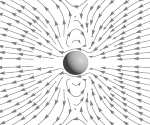
We now analyse in detail the case where the two motions are in phase,  $\zeta = 0$; other phase differences show similar trends but at reduced frequencies; figure 1(c). Figure 2(a–f) shows the pathlines of the net-force flow (2.9b), in the $z$–
$z$– $x$ plane at $y=0$, at dimensionless frequencies $\beta = 10,16.817,25,29.080,35,50$; note that this flow is axisymmetric about the $z$-axis. These values of $\beta$ are chosen to highlight typical flow fields at, above and below the two bifurcations.

Figure 2. (a–f) Cycle-averaged pathlines at values of  $\beta$ selected to illustrate the different regimes. Pathlines are plotted in the $z$–
$z$– $x$ plane but are axisymmetric about the $z$-axis. The stagnation points of the flow are given by dots. (g) Bifurcation diagram of $\beta$ vs the $r$ values (spherical radial coordinate) where the stagnation points occur. Dots coincide with those reported in (a–f). All results correspond to $\zeta = 0$.
Two distinct bifurcations occur at different values of  $\beta$; the first bifurcation occurs at $\beta = 16.817$, and the second coincides with $\beta _{reversal} = 29.080$. At frequencies below the first bifurcation, all cycle-averaged pathlines move in the negative $z$-direction; figure 2(a). At the first bifurcation, a stagnation point forms at a radius of $r = 2.1736$; figure 2(b). As $\beta$ increases, the stagnation point then splits into a saddle node and a vortex centre; see figure 2(c). As $\beta$ continues to increase, the vortex centre moves towards the sphere while the saddle node moves away from the sphere. The saddle node continues to move away from the sphere until it vanishes at $\beta _{reversal}= 29.080$, at which point the vortex encompasses the entire domain, i.e. all pathlines are closed. The pathlines exhibit a similar structure to a source dipole, decaying at a rate of $1/r^3$, and results in $F_{net}=0$; figure 2(d). As $\beta$ increases above $\beta _{reversal}$, a boundary emerges, which separates an inner vortex from an outer region. In the asymptotic limit as $\beta \rightarrow \infty$, the outer flow becomes independent of $\beta$, aligning with calculations of different streaming flows in this limit, e.g. Riley (Reference Riley1966). The pathlines in this outer region move in the opposite direction to those in the outer region for $\beta < \beta _{reversal}$. As we shall show in § 3.2, this drives the change in direction of $F_{net}$. See Bhosale, Parthasarathy & Gazzola (Reference Bhosale, Parthasarathy and Gazzola2020) and Chan et al. (Reference Chan, Bhosale, Parthasarathy and Gazzola2022) for further discussion on the bifurcations that occur in related viscous streaming flows.
3.2. Connection between  $F_{net}$ and the far-field flow

The exact solution for the steady streaming flow, (2.9), has the form of a multipole expansion. We therefore obtain the flow in the far field by keeping only the slowest decaying terms as  $r\rightarrow \infty$. This shows that far from the particle, the flow is that of a Stokeslet with strength $F_{net}$:
 \begin{gather} \bar{p}^{(1)} \sim{-}\frac{\boldsymbol{r}}{4{\rm \pi}|\boldsymbol{r}|^3} \cdot F_{net}\boldsymbol{k},\quad |\boldsymbol{r}|\rightarrow \infty, \end{gather}
 \begin{gather}\bar{\boldsymbol{u}}^{(1)} \sim{-}\frac{1}{8{\rm \pi}}\left(\frac{\boldsymbol{\mathsf{I}}}{|\boldsymbol{r}|}+\frac{\boldsymbol{r} \boldsymbol{r}}{|\boldsymbol{r}|^3}\right)\cdot F_{net}\boldsymbol{k},\quad |\boldsymbol{r}|\rightarrow \infty, \end{gather}
where  $\boldsymbol{\mathsf{I}}$ is the identity tensor and $F_{net}$ is defined in (2.14). Note that the oscillatory disturbances, and components of the steady flow that do not lead to a net force, have velocity fields which decay faster than $1/r$. This establishes that the bifurcation that switches the direction of the far-field pathlines switches the direction of the Stokeslet which is connected to $F_{net}$ by (3.1).
4. Discussion and conclusions
We have investigated the origin of the reversal in the direction of acoustically propelled nanoparticles by examining a model problem of a sphere performing oscillatory rotations in a rectilinearly oscillating velocity field. This sheds light on the flow field that drives acoustic propulsion which is yet to be reported; the Lorentz reciprocal theorem is usually used instead. This revealed two distinct bifurcations that result in a change to the direction of the pathlines in the far field at a critical value of the dimensionless frequency, which directly leads to the reversal in the net hydrodynamic force on the particle.
This connection between the far-field pathlines and the net force was facilitated by showing the far-field flow exactly corresponds to an equivalent Stokeslet. The equivalent Stokeslet representation of the far-field streaming flow is not unique to solid particles with spherical geometries. Using the boundary integral formulation of Stokes flows and performing a multipole expansion, it can be shown that the leading-order multipole is always a Stokeslet; this is due to the fast decay of the body force in (2.5a). The strength of the Stokeslet, however, will in general not be given by  $F_{net}$ for non-spherical bodies; this is because the net force will in general include effects due to the Lagrangian motion of the particle, e.g. Collis et al. (Reference Collis, Chakraborty and Sader2022).
Given many acoustic propulsion experiments use suspensions of particles (Wang et al. Reference Wang, Castro, Hoyos and Mallouk2012; Ahmed et al. Reference Ahmed, Gentekos, Fink and Mallouk2014), it is of interest to investigate at what distance the flow can be replaced by its equivalent Stokeslet. This could alleviate the need to calculate the complex nature of the flow field in the vicinity of each particle when performing computational simulations of these suspensions. Figure 3(a–f) gives the streaming flow, equivalent Stokeslet, and relative difference between these flows for  $\beta = 25$ and $\beta = 50$, which are below and above $\beta _{reversal} = 29.080$, respectively. As expected, the difference vanishes as $r\rightarrow \infty$; figure 3(c,f). Figure 3(g) shows the minimum radial distance from the sphere where the difference is 10 % or less. When $\beta \rightarrow \beta _{reversal}$, this difference diverges as the net force vanishes and there is no equivalent Stokeslet at the reversal frequency. As the flow field at $\beta _{reversal}$ resembles a source dipole in the particle's far field, inclusion of this multipole may improve the overall accuracy of the singularity representation of the flow field. Acoustically propelled particles are confined to a two-dimensional plane, i.e. the pressure node, and thus suspensions of such particles provide an intriguing set-up for investigating collective dynamics. Considering these suspensions as a superposition of singularity solutions, confined to lie in a monolayer, provides direct access to the vast array of literature on collective dynamics in Stokes flows (Elgeti, Winkler & Gompper Reference Elgeti, Winkler and Gompper2015), including applications such as tracer diffusion in suspensions of active particles (Leptos et al. Reference Leptos, Guasto, Gollub, Pesci and Goldstein2009) and phase behaviour and rheology of dense active colloids (Ishikawa, Brumley & Pedley Reference Ishikawa, Brumley and Pedley2021).

Figure 3. (a–f) Net-force flow (pathlines), equivalent Stokeslet (pathlines) and relative error between the two flows for  $\beta = 25$ and $\beta = 50$; $\zeta = 0$ in both cases. The colour bar gives the flow magnitude with the dimensionless angular velocity, $\alpha$, scaled out. (g) Minimum bound on the (spherical) radial distance, r, from the origin where the error is 10 % or less.
Supplementary material
Supplementary material is available at https://doi.org/10.1017/jfm.2024.217.
Funding
The authors acknowledge the support of the Melbourne Research Scholarship.
Declaration of interests
The authors report no conflict of interest.


 Open access