


1. Introduction
The convection obtained by heating from below, known as the Rayleigh–Bénard convection because of the pioneering studies of Bénard (Reference Bénard1901) and Rayleigh (Reference Rayleigh1916), has been widely studied, first for theoretical reasons as the analysis of pattern formation and then for its great interest in practical applications, as for example crystal growth (see the references in Lappa Reference Lappa2007) and thermal convection in the Earth's mantle (Baumgardner Reference Baumgardner1985). The first studies rather concerned infinitely extended layers for which analytical derivations could be performed (Chandrasekhar Reference Chandrasekhar1961), but studies in confined enclosures have also been developed in connection with practical applications and with the progress in numerical computing (Meneguzzi et al. Reference Meneguzzi, Sulem, Sulem and Thual1987). In such situations, a critical Rayleigh number  ${Ra}_c$ has to be reached for the onset of flow, and subsequent flow bifurcations, either steady or oscillatory, can occur before a chaotic state is reached, which gives a very interesting flow dynamics (Bodenschatz, Pesch & Ahlers Reference Bodenschatz, Pesch and Ahlers2000). The dynamics is particularly rich in confined situations, where geometry effects and boundary conditions play an important role and where symmetry considerations are involved (Cliffe & Winters Reference Cliffe and Winters1986). Numerical linear stability analyses were first carried out to determine the variation of ${Ra}_c$ with the aspect ratio of the cavity (Catton Reference Catton1970; Charlson & Sani Reference Charlson and Sani1970). For further nonlinear study, numerical methods using the parameter continuation and bifurcation methods proved to be very efficient. In the case of parallelepipedic situations, very interesting results are reported by Puigjaner et al. (Reference Puigjaner, Herrero, Giralt and Simó2004, Reference Puigjaner, Herrero, Giralt and Simó2006, Reference Puigjaner, Herrero, Simó and Giralt2008): detailed bifurcation diagrams give the development of the steady flow patterns inside a cubic cavity heated from below with either adiabatic or conducting lateral walls and filled either with air ( ${Pr} = 0.71$) or silicone oil ( ${Pr} = 130$). Different flow patterns are found to be stable in the same ${Ra}$ range. These bifurcation diagrams allow us to explain the transitions between different steady flow patterns observed experimentally by Pallares et al. (Reference Pallares, Arroyo, Grau and Giralt2001) in a cubic cavity filled with silicone oil. More recently, Torres et al. (Reference Torres, Henry, Komiya, Maruyama and Ben Hadid2013, Reference Torres, Henry, Komiya and Maruyama2014) studied the perturbations induced to the bifurcation diagrams by imposing a small tilt to such three-dimensional cavities.
All these aforementioned studies generally refer to Newtonian fluids, i.e. fluids in which the viscous shear stress is proportional to the shear rate, with a constant of proportionality which is the viscosity. However, the liquids involved in many engineering applications and in some geophysical phenomena very often present more complex rheological behaviours. We can mention the viscoplastic rheology often associated with geophysical flows, where the fluids generally behave as shear-thinning liquids with a yield stress. For the sake of simplicity, the latter effect is often not taken into account, and generalized Newtonian fluids are considered, where the viscosity remains a scalar but varies with the local shear rate (decreasing for a shear-thinning fluid and increasing for a shear-thickening fluid), giving a more complex nonlinear relationship between shear stress and shear rate. A typical model for such fluids is the Carreau inelastic model giving the viscosity as a function of the shear rate with a four-parameter expression, or the simplified and more tractable power-law model, each of these models involving the power-law index  $n$.
$n$.
The first theoretical investigations considered power-law fluids. Tien, Tsuei & Sun (Reference Tien, Tsuei and Sun1969) investigated the linear threshold of convection in a horizontal layer heated from below, using the energy approach developed by Chandrasekhar (Reference Chandrasekhar1961) for a Newtonian fluid. They wrongly predicted the dependence of the critical Rayleigh number  ${Ra}_c$ with the power-law index $n$, as shown later by Khayat (Reference Khayat1996). The reason is the inability of the power-law model to predict viscosity at low shear rate, with a singularity for shear-thinning fluids and a zero value for shear-thickening fluids in place of the Newtonian value. Because of its simplicity, this model was also used in two-dimensional (2-D) numerical simulations, particularly in rigid rectangular cavities. Inaba, Dai & Horibe (Reference Inaba, Dai and Horibe2003) performed simulations in long 2-D cavities in connection with phase-change-material slurries and established correlations between the heat transfer expressed by the Nusselt number and the governing parameters. Turan et al. (Reference Turan, Fotso-Choupe, Lai, Poole and Chakraborty2014) considered a square enclosure with either a prescribed temperature or a prescribed thermal flux at the horizontal boundaries. Thanks to simulations initiated from Newtonian steady states, they give the variations of the flow onset (smallest Rayleigh number for which a convective solution is obtained), flow characteristics and Nusselt number as a function of the power-law index $n$. They obtain a decrease of the flow onset for $n<1$, but also detect variations of this onset, based on small ${Nu}$ deviations from unity, for $n>1$. Yigit, Poole & Chakraborty (Reference Yigit, Poole and Chakraborty2015) then extended the study to rectangular enclosures with different aspect ratios. Numerical simulations in 2-D rigid cavities have also been done by Benouared, Mamou & Ait Messaoudene (Reference Benouared, Mamou and Ait Messaoudene2014) with the Carreau model. They interestingly consider long cavities in which, for imposed heat fluxes at the lower and upper boundaries, the flow takes the form of a single long-size roll. Such flow can be either numerically simulated in two dimensions, or obtained by a simpler asymptotic approach based on the parallel flow approximation. In that way, they were able to get a precise description of the subcritical branches obtained for sufficiently shear-thinning fluids. They also considered a square cavity with either constant heat fluxes or constant temperatures at the horizontal boundaries.
The Carreau model has also been used to study the Rayleigh–Bénard dynamics in extended layers of non-Newtonian fluids. Khayat (Reference Khayat1996) examined the influence of weak shear thinning on the development of chaos in a layer heated from below and with lower and upper stress-free surfaces, generalizing the classical Lorenz system. He found that the critical Rayleigh number for the linear onset of flow is the same as for a Newtonian fluid, but the flow development until chaos is dramatically altered by shear thinning. This study based on the planar convection hypothesis is later extended to 3-D flow structures by Albaalbaki & Khayat (Reference Albaalbaki and Khayat2011). Linear and weakly nonlinear analyses show that, if rolls are preferred for shear-thickening fluids as in the Newtonian case, rolls, squares or hexagons can be obtained for shear-thinning fluids on supercritical and subcritical branches, and the preferred structure on the supercritical branches depends on the shear-thinning level. Bouteraa et al. (Reference Bouteraa, Nouar, Plaut, Metivier and Kalck2015) also performed a weakly nonlinear analysis of the same configuration, but assumed variable slip conditions on the lower and upper boundaries, from no slip to stress free, and focused on shear-thinning fluids. They determined the degree of shear-thinning parameter  $\alpha$ above which the bifurcation becomes subcritical and found smaller values than Albaalbaki & Khayat (Reference Albaalbaki and Khayat2011). They also found that, in the supercritical regime, only rolls are stable near onset. This work is further extended to situations with upper and lower boundaries of arbitrary conductivity (Bouteraa & Nouar Reference Bouteraa and Nouar2015, Reference Bouteraa and Nouar2016).
Two-dimensional simulations of the Rayleigh–Bénard flow in non-Newtonian fluids have also been performed in periodic square or almost square cavities. The idea is to simulate one roll in a regular pattern inside an extended geometry. Considering a shear-thinning power-law fluid in a square cavity, Ozoe & Churchill (Reference Ozoe and Churchill1972) determined the smallest Rayleigh number at which a solution can be sustained, an approximation of the saddle-node point on the subcritical branch. This value was found to decrease when the shear-thinning properties were amplified. Parmentier (Reference Parmentier1978) took a similar approach and studied in detail nonlinear convection rolls above their subcritical onset in shear-thinning power-law fluids. He introduced a volume-average viscosity (weighted by the square of the shear rate) that allows us to define a new Rayleigh number, known as the Parmentier–Rayleigh number. Expressed as a function of that new Rayleigh number, the variation of the heat transfer (expressed with the Nusselt number) for the convection rolls in shear-thinning conditions can appear as a single universal curve, which is the one obtained for Newtonian fluids. Benouared et al. (Reference Benouared, Mamou and Ait Messaoudene2014) simulated a similar square cavity situation with the Carreau model. For different values of the power-law index  $n$, they gave the stable part of the subcritical branches, down to the saddle-node point. Finally Jenny, Plaut & Briard (Reference Jenny, Plaut and Briard2015) considered a similar problem in an almost square cavity, choosing a length corresponding to the critical length for one roll. For a large range of rheological parameters, they computed the stable roll solutions along the subcritical branches in shear-thinning Carreau fluids. They obtained an interesting simple expression for the value of the Rayleigh number at which subcritical rolls appear. They also proposed a correlation to estimate the Nusselt number of these subcritical rolls.
We did not find any paper related to 3-D simulations of such Rayleigh–Bénard flows in generalized Newtonian fluids, such as shear-thinning fluids, inside confined 3-D cavities. Moreover, such studies involving the calculation of subcritical branches would benefit from the possibility of using continuation methods. This led us to adapt a 3-D spectral finite element code using continuation and developed for Newtonian fluids to study the Rayleigh–Bénard convection in a non-Newtonian fluid inside a parallelepiped enclosure. The 3-D cavity we consider has moderate dimensions (its length is equal to twice the size of the square cross-section), allowing reasonable computing times. Already used by Torres et al. (Reference Torres, Henry, Komiya, Maruyama and Ben Hadid2013) to study the effect of a tilt imposed on the cavity, it offers a relatively simple flow dynamics in the case without tilt, with two stable solutions in the Newtonian case, a solution with one longitudinal roll and a solution with two transverse rolls. In such a cavity, the modifications induced by the non-Newtonian properties are expected to be more clearly depicted. Non-Newtonian Carreau fluids with either shear-thinning or shear-thickening properties are considered. For this problem, we first recall the results obtained in the Newtonian case and then put into light the changes affecting the flow dynamics of the stable branches when shear-thinning or shear-thickening fluids are considered. Order of magnitude and energy analyses at the thresholds are also proposed, as well as comparisons with previous studies.
2. Mathematical model and numerical techniques
2.1. Mathematical model
The mathematical model consists of a parallelepiped cavity filled with a non-Newtonian fluid which is differentially heated. The cavity has aspect ratios  $A_z=l/h=2$ and $A_y=w_d/h=1$, where $l$ is the length of the cavity (along $z^*$), $h$ is its height (along $x^*$) and $w_d$ is its width (along $y^*$), as shown schematically in figure 1. The origin of the system of coordinates is placed at the centre of the cavity and its axes are parallel to the edges of the truncated square duct. The coordinates ( $x^*,y^*,z^*$) are then normalized by $h$ to obtain ( $x,y,z$). The lower and upper walls corresponding to $yz$-planes at $x=-1/2$ and $x=1/2$, respectively, are isothermal and held at different temperatures, $T^*_H$ for the lower wall and $T^*_C$ for the upper wall, with $T^*_H > T^*_C$, whereas the other walls are adiabatic. All the boundaries are rigid walls with no-slip conditions. The non-Newtonian fluid is assumed to follow the four-parameter Carreau inelastic model, i.e. its dynamic viscosity varies with the shear rate, from the value at zero shear rate to the asymptotic value at infinite shear rate, with an intermediate power-law variation. Such a viscosity $\mu _c$ following the Carreau model can be expressed as
 \begin{equation} \frac{\mu_c-\mu_\infty}{\mu_0-\mu_\infty}=[1+(\delta |\dot{\gamma}^*_{\boldsymbol u}|)^2]^{(n-1)/2}, \end{equation}
where  $\mu _0$ and $\mu _\infty$ are the limit Newtonian dynamic viscosities at zero and infinite shear rate, respectively, $n$ is the power-law index, $\delta$ is a characteristic time of the fluid and $\dot {\gamma }^*_{\boldsymbol u}$ is the shear rate expressed as
 \begin{equation} \dot{\gamma}^*_{\boldsymbol u,ij}=\left(\frac{\partial u^*_i}{\partial x^*_j}+\frac{\partial u^*_j}{\partial x^*_i}\right), \end{equation}
from which the shear stress  $\sigma ^*_{ij}=\mu _c \dot {\gamma }^*_{\boldsymbol u,ij}$ can be obtained. In the expression of the shear rate, $x^*_i$ and $u^*_i$ ( $i=1,3$) are the coordinates and velocities in the different directions. Note that $1/\delta$ gives the characteristic shear rate at which the viscosity $\mu _c$ starts to decrease below the Newtonian plateau at $\mu _0$. Using $\mu _0$ to normalize the viscosity and $\kappa /h^2$ ( $\kappa$ is the thermal diffusivity) to normalize the shear rate, and defining $I$ as $\mu _\infty /\mu _0$, we can also write
 \begin{equation} \frac{\mu_c}{\mu_0}= I + (1 - I) [1+( L |\dot{\gamma}_{\boldsymbol u}|)^2]^{(n-1)/2}, \end{equation}
or
 \begin{equation} \frac{\mu_c}{\mu_0}= [1+( L |\dot{\gamma}_{\boldsymbol u}|)^2]^{(n-1)/2}, \end{equation}
if we assume  $\mu _\infty =0$, as will be done in this study. In these expressions, $L=\delta \kappa /h^2$ is the dimensionless characteristic time and $\dot {\gamma }_{\boldsymbol u}$ is the dimensionless shear rate. Note that Bouteraa et al. (Reference Bouteraa, Nouar, Plaut, Metivier and Kalck2015), in a weakly nonlinear analysis, have shown that, for a shear-thinning fluid, the nature of the bifurcation from the conduction state to convection rolls depends on a single rheological parameter, quantifying the degree of shear thinning,
 \begin{equation} \alpha = \tfrac{1}{2} (1-n) L^2, \end{equation}
which, in fact, controls the magnitude of the first nonlinear term in the development of the dimensionless viscosity (2.4) with respect to the shear rate. Finally, the Carreau dynamic viscosity can also be expressed as  $\mu _c=\mu _0(1+\mu )$, where $\mu$ is the dimensionless departure from the dynamic viscosity at zero shear rate. Using (2.4), $\mu$ can be expressed as
 \begin{equation} \mu=([1+(L |\dot{\gamma}_{\boldsymbol u}|)^2]^{(n-1)/2}-1). \end{equation}
The other physical properties of the fluid (thermal diffusivity  $\kappa$, density $\rho$) will be assumed constant, except that, according to the Boussinesq approximation, the fluid density is considered as temperature dependent in the buoyancy term with a linear law $\rho =\rho _m (1-\beta (T^* - T^*_m))$, where $\beta$ is the thermal expansion coefficient and $T^*_m$ is a reference temperature taken as the mean temperature $(T^*_H + T^*_C)/2$.

Figure 1. Geometry of the dimensionless heated truncated square duct. The cross-section of the duct is a unit square and its length is 2. The two walls corresponding to  $yz$-planes at $x=-1/2$ and $x=1/2$ are isothermal and held at $T_H=1/2$ and $T_C=-1/2$, respectively. The other walls are adiabatic.
The convective motions are then modelled by the Navier–Stokes equations coupled to an energy equation. Using  $h$,
$h$,  $h^2 / \kappa$, $\kappa / h$, $\rho _m \kappa ^2 / h^2$ and $\Delta T^*=(T^*_H-T^*_C)$ as scales for length, time, velocity, pressure and temperature, respectively, these equations take the following form:
 \begin{gather} \boldsymbol{\nabla} \boldsymbol{\cdot} {\boldsymbol u} = 0, \end{gather}
 \begin{gather}\frac{\partial{\boldsymbol u}}{\partial t} + ({\boldsymbol u}\boldsymbol{\cdot}\boldsymbol{\nabla}){\boldsymbol u} ={-}\boldsymbol{\nabla} p + {Pr} \, \boldsymbol{\nabla} \boldsymbol{\cdot} ((1+\mu(\boldsymbol u))\dot{\gamma}_{\boldsymbol u}) + {Pr} \, {Ra} \, T {\boldsymbol e_x} , \end{gather}
 \begin{gather}\frac{\partial T} {\partial t} + ({\boldsymbol u}\boldsymbol{\cdot}\boldsymbol{\nabla}) T = \nabla^2 T, \end{gather}
with boundary conditions given by  $T = 1/2$ on $x= -1/2$ and $T = -1/2$ on $x=1/2$, $\partial T/\partial z =0$ on $z=-1$, $1$ and $\partial T/\partial y =0$ on $y=-1/2$, $1/2$ and ${\boldsymbol u}=0$ on all the boundaries. The dimensionless variables are the velocity vector ${\boldsymbol u}=(u,v,w)$, the pressure $p$ and the temperature $T=(T^*-T^*_m)/(T^*_H-T^*_C)$. Here, ${\boldsymbol e_x}$ is the unit vector in the vertical $x$ direction. Note that $\mu$ is written as $\mu (\boldsymbol u)$ to express that it depends on the velocity $\boldsymbol u$ through the shear rate (see (2.6)). The non-dimensional parameters are the Rayleigh number, ${Ra}=\beta \Delta T^* g h^3 / (\kappa \nu _0)$ and the Prandtl number, ${Pr}= \nu _0 / \kappa$, where $\nu _0$ is the kinematic viscosity defined as $\nu _0=\mu _0/\rho _m$ and $g$ is the gravitational acceleration. We can also define the Nusselt number ${Nu}$, which expresses the actual heat transfer through $yz$-planes compared with the diffusive heat transfer. Due to the adiabatic sidewalls, ${Nu}$ is the same for all $yz$-planes. It can be written simply in our case as ${Nu}=\int _{y,z} \, (-{\rm d}T/{{\rm d}\kern0.7pt x})/2 \, {{\rm d} y} \, {\rm d}z$ and will be calculated at the upper wall for $x=1/2$.
Under the approximation of the model, the basic no-flow solution presents different symmetries: reflection symmetries  $S_{P_{yz}}$, $S_{P_{xz}}$ and $S_{P_{xy}}$ with respect to the three middle planes (horizontal $yz$-plane, longitudinal vertical $xz$-plane and transverse vertical $xy$-plane, respectively), which, by combination, induce ${\rm \pi}$-rotational symmetries $S_{A_x}$, $S_{A_y}$ and $S_{A_z}$ about the three middle axes (vertical $x$-, transverse $y$- and longitudinal $z$-axes, respectively). These symmetries belong to a $Z_2 \times Z_2 \times Z_2$ group. As an example, we define two of these symmetries, $S_{P_{xy}}$ and $S_{A_z}$, and the others can be obtained by circular permutation
 \begin{gather} S_{P_{xy}} :\quad (x,y,z,t) \rightarrow (x,y,-z,t), \quad (u,v,w,T) \rightarrow (u,v,-w,T), \end{gather}
 \begin{gather}S_{A_z} : \quad (x,y,z,t) \rightarrow ({-}x,-y,z,t), \quad (u,v,w,T) \rightarrow ({-}u,-v,w,-T). \end{gather}
The symmetry  $S_C$ with respect to the centre point of the cavity can also be obtained by combination of the previous symmetries. If all these symmetries are those of the basic no-flow solution, the effective symmetries of the flow solutions will depend on the flow configuration triggered. Moreover, when increasing ${Ra}$, bifurcations to new flow states (steady or oscillatory) will occur, at which some of the symmetries will usually be broken.
2.2. Numerical techniques
The governing equations of the model are solved in the 3-D domain using a spectral element method, as described in Ben Hadid & Henry (Reference Ben Hadid and Henry1997). The spatial discretization is obtained through Lagrange polynomials with Gauss–Lobatto–Legendre point distributions; the time discretization is carried out using a semi-implicit splitting scheme where, as proposed by Karniadakis, Israeli & Orszag (Reference Karniadakis, Israeli and Orszag1991), the nonlinear terms are first integrated explicitly, the pressure is then solved through a pressure equation enforcing the incompressibility constraint (with a consistent pressure boundary condition derived from the equations of motion), and the linear terms are finally integrated implicitly, using the very efficient matrix solver by diagonalization of the operator along each of the space directions. In its first-order formulation, this time integration scheme is used for steady-state solutions (Mamun & Tuckerman Reference Mamun and Tuckerman1995), eigenvalue and eigenvector calculation and determination of bifurcation points (Bergeon et al. Reference Bergeon, Henry, Ben Hadid and Tuckerman1998; Petrone, Chénier & Lauriat Reference Petrone, Chénier and Lauriat2004) through a Newton method, as it is described in Torres et al. (Reference Torres, Henry, Komiya, Maruyama and Ben Hadid2013). The overall continuation strategy is also well explained in Torres et al. (Reference Torres, Henry, Komiya and Maruyama2014). Such methods, originally developed for Newtonian fluids, had to be adapted to deal with Carreau fluids. These adaptations are described in the following, after a brief summary of the Newtonian case approach.
In the Newtonian case, the first-order time scheme is written in the abbreviated form
 \begin{equation} \frac{\boldsymbol{X}^{(k+1)}-\boldsymbol{X}^{(k)}} {\Delta t} = {\mathcal{N}} (\boldsymbol{X}^{(k)},{Ra}) + {\mathcal{L}} \boldsymbol{X}^{(k+1)}, \end{equation}
which, for large  $\Delta t$, can also be expressed as
 \begin{equation} {{\boldsymbol{X}^{(k+1)}-\boldsymbol{X}^{(k)}}} ={-} {\mathcal{L}}^{{-}1} [{\mathcal{N}}(\boldsymbol{X}^{(k)},{Ra}) + {\mathcal{L}} \boldsymbol{X}^{(k)}] . \end{equation}
In these expressions,  $\boldsymbol {X}$ denotes all of the spatially discretized fields $({\boldsymbol {u}}(u,v,w), T)$, ${\mathcal {N}}$ is the spatially discretized nonlinear operator (including pressure and buoyancy terms) and ${\mathcal {L}}$ is the spatially discretized linear operator corresponding to the Laplacian operator (viscous or diffusive terms). If we consider the steady-state problem expressed as
 \begin{equation} {\mathcal{N}}(\boldsymbol{X},{Ra}) + {\mathcal{L}} \boldsymbol{X}=0, \end{equation}
and want to solve it with a Newton method, each Newton step, preconditioned with the operator  $- {\mathcal {L}}^{-1}$, can be written as
 \begin{equation} \left.\begin{array}{c@{}} -{\mathcal{L}}^{{-}1} [{\mathcal{N}}_{\boldsymbol{X}}(\boldsymbol{X},{Ra}) + {\mathcal{L}} ] \delta \boldsymbol{X} ={-}(-{\mathcal{L}}^{{-}1}) [{\mathcal{N}}(\boldsymbol{X},{Ra}) + {\mathcal{L}} \boldsymbol{X}],\\ \boldsymbol{X} \leftarrow \boldsymbol{X} + \delta \boldsymbol{X}, \end{array}\right\} \end{equation}
where  ${\mathcal {N}}_{\boldsymbol {X}}(\boldsymbol {X},{Ra})$ is the Jacobian of ${\mathcal {N}}$ with respect to $\boldsymbol {X}$ evaluated at $\boldsymbol {X}$ and ${Ra}$. If we solve the linear system (2.15) by an iterative method, we need only provide the right-hand side and the action of the matrix-vector product constituting the left-hand side. Referring to (2.13), we see that the right-hand side of (2.15) can be obtained by carrying out a time step, and the matrix-vector product by carrying out a linearized version of the same time step. The Jacobian matrix is thus never constructed or stored. The generalized minimal residual (GMRES) algorithm from the NSPCG software library (Oppe, Joubert & Kincaid Reference Oppe, Joubert and Kincaid1989) is used as the iterative solver.
In the case of the Carreau fluid, the viscous term is no longer a simple Laplacian operator. A first possibility we have tested is to calculate the new viscous discretized operator. This operator, however, depends on the local velocities through the viscosity and the shear rate, so that it has to be regularly recalculated at each Newton step. Moreover, with this operator, we cannot use the very efficient diagonalization solver for the velocity at each time step, which is a real handicap to the solution of large 3-D problems. Following the idea of Karamanos & Sherwin (Reference Karamanos and Sherwin2000), we finally chose another possibility, which is to write the viscous term in (2.8) as
 \begin{equation} \boldsymbol{\nabla} \boldsymbol{\cdot} ((1+\mu({\boldsymbol u}))\dot{\gamma}_{\boldsymbol u})=\nabla^2 {\boldsymbol u^{(k+1)}} + \boldsymbol{\nabla} \boldsymbol{\cdot} (\mu({\boldsymbol u^{(k)}}) \dot{\gamma}_{\boldsymbol u^{(k)}}). \end{equation}
With this choice, we keep  ${\mathcal {L}}$ as the Laplacian and the other term $\boldsymbol {\nabla }\boldsymbol {\cdot } (\mu ({\boldsymbol u^{(k)}}) \dot {\gamma }_{\boldsymbol u^{(k)}})$ is added in the nonlinear terms ${\mathcal {N}}$ considered at the known step $k$. We also have to consider the viscous term of the linearized time step that allows us to calculate the correction $\delta \boldsymbol u$ of $\boldsymbol u$ on the left-hand side of (2.15). It can be written as
 \begin{align} \delta(\boldsymbol{\nabla} \boldsymbol{\cdot} ((1+\mu({\boldsymbol u}))\dot{\gamma}_{\boldsymbol u}))&=\nabla^2 \delta {\boldsymbol u^{(k+1)}} + \boldsymbol{\nabla} \boldsymbol{\cdot} (\mu({\boldsymbol u^{(k)}}) \dot{\gamma}_{\delta \boldsymbol u^{(k)}}) \nonumber\\ &\quad + \boldsymbol{\nabla} \boldsymbol{\cdot} ((\partial \mu/\partial \boldsymbol u){\delta \boldsymbol u^{(k)}} \dot{\gamma}_{\boldsymbol u^{(k)}}). \end{align}
The two last terms are included in  ${\mathcal {N}}_{\boldsymbol {X}}$ during the Newton step, which is otherwise unchanged and keeps the form given in (2.15). Compared with the Newtonian case, the fact that parts of the viscous operator are taken explicitly can slightly slow down the Newton convergence, but the use of the diagonalization solver allows us to keep reasonable overall computing times.
Note that other developments of the viscous term are needed, in particular for the calculation of the bifurcation points, which involves the solution of the linearized equation for the eigenvector at threshold by a Newton method (such a solution in the Newtonian case can be found in Torres et al. Reference Torres, Henry, Komiya, Maruyama and Ben Hadid2013). If the velocity eigenvector is denoted as  ${\boldsymbol u_p}$, in the linearized equation for the eigenvector we will have a viscous term similar to (2.17) and expressed as
 \begin{equation} \nabla^2 {\boldsymbol u_p^{(k+1)}} + \boldsymbol{\nabla} \boldsymbol{\cdot} (\mu({\boldsymbol u^{(k)}}) \dot{\gamma}_{\boldsymbol u_p^{(k)}}) + \boldsymbol{\nabla} \boldsymbol{\cdot} ((\partial \mu/\partial \boldsymbol u){\boldsymbol u_p^{(k)}} \dot{\gamma}_{\boldsymbol u^{(k)}}). \end{equation}
The viscous term corresponding to the Jacobian equation used to solve the equation for the eigenvector with a Newton method is still more complex. This viscous term involves the corrections  $\delta \boldsymbol u_p$ of the velocity eigenvector and $\delta \boldsymbol u$ of the velocity and can be expressed as
 \begin{align} &\nabla^2 \delta {\boldsymbol u_p^{(k+1)}} + \boldsymbol{\nabla} \boldsymbol{\cdot} (\mu({\boldsymbol u^{(k)}}) \dot{\gamma}_{\delta \boldsymbol u_p^{(k)}}) + \boldsymbol{\nabla} \boldsymbol{\cdot} ((\partial \mu/\partial \boldsymbol u){\delta \boldsymbol u_p^{(k)}} \dot{\gamma}_{\boldsymbol u^{(k)}}) \nonumber\\ &\quad + \boldsymbol{\nabla} \boldsymbol{\cdot}((\partial \mu/\partial \boldsymbol u){\delta \boldsymbol u^{(k)}} \dot{\gamma}_{\boldsymbol u_p^{(k)}}) + \boldsymbol{\nabla} \boldsymbol{\cdot} ((\partial \mu/\partial \boldsymbol u){\boldsymbol u_p^{(k)}} \dot{\gamma}_{ \delta \boldsymbol u^{(k)}}) \nonumber\\ &\quad + \boldsymbol{\nabla} \boldsymbol{\cdot} ((\partial^2 \mu/\partial^2 \boldsymbol u){{ \delta \boldsymbol u^{(k)}} \boldsymbol u_p^{(k)}} \dot{\gamma}_{\boldsymbol u^{(k)}}). \end{align}
We see that many different terms must then be taken into account. In our formulation, except for the first Laplacian term, they are all considered at the known step  $k$ and added to the nonlinear terms. Despite all these new terms, which make the Newton steps more complex, we generally also keep a good convergence of the bifurcation points with the Carreau model.
3. Results
Our results concern the convective flows induced in Carreau fluids in a cavity with  $A_y=1$ (square $xy$-cross-section) and $A_z=2$, and for ${Pr}=1$. We will assume that $\mu _\infty =0$ ( $I=0$) and the focus will be first on shear-thinning fluids ( $n < 1$) for which the viscosity decreases with the increase of the shear rate. In a second step, we will consider shear-thickening fluids ( $n > 1$) for which the viscosity increases with the increase of the shear rate.
3.1. Discussion on the choice of the parameters
As presented in the introduction, shear-thinning fluids have been considered in many studies (for example, Albaalbaki & Khayat Reference Albaalbaki and Khayat2011; Benouared et al. Reference Benouared, Mamou and Ait Messaoudene2014; Bouteraa et al. Reference Bouteraa, Nouar, Plaut, Metivier and Kalck2015; Bouteraa & Nouar Reference Bouteraa and Nouar2015, Reference Bouteraa and Nouar2016; Jenny et al. Reference Jenny, Plaut and Briard2015; Yigit et al. Reference Yigit, Poole and Chakraborty2015; Darbouli et al. Reference Darbouli, Métivier, Leclerc, Nouar, Bouteera and Stemmelen2016). Benouared et al. (Reference Benouared, Mamou and Ait Messaoudene2014) give the Carreau parameters for typical non-Newtonian fluids, xanthan gum, carboxymethylcellulose, polyacrylamide:  $0.484 \leq n \leq 0.673$, $9 \times 10^{-4} \leq I \leq 9 \times 10^{-2}$, $0.0125 \leq \delta \leq 45.8$ s. The dimensionless time parameter $L$ cannot be obtained as the values of the thermal diffusivity $\kappa$ are not given and a characteristic length is also needed. Looking through the different studies, we find that the parameters generally used are $0.4 \leq n \leq 1$, 0 or small values for $I$ and $0 \leq L \leq 0.8$. The range of $L$ can be extended to large values, up to $L=200$, as in Jenny et al. (Reference Jenny, Plaut and Briard2015). Following these studies, we decided to choose $I=0$, $0 \leq L \leq 1$ and $0.5 \leq n \leq 1$. Besides, for shear-thickening fluids, we chose $1 \leq n \leq 1.5$.
Concerning the Prandtl number, Albaalbaki & Khayat (Reference Albaalbaki and Khayat2011) indicate that most of the fluids displaying shear-thinning behaviour such as polymeric melts and solutions are characterized by a high Prandtl number, but other fluids of a low Prandtl number such as low-temperature monoatomic liquids also exhibit shear thinning. They then chose to study a large range of Prandtl number,  $5 \times 10^{-2} \leq {Pr} \leq 10^3$. Yigit et al. (Reference Yigit, Poole and Chakraborty2015) and Darbouli et al. (Reference Darbouli, Métivier, Leclerc, Nouar, Bouteera and Stemmelen2016) rather focus on large values such as ${Pr}=1000$. Benouared et al. (Reference Benouared, Mamou and Ait Messaoudene2014) and Jenny et al. (Reference Jenny, Plaut and Briard2015) chose moderate values, ${Pr}=10$ and ${Pr}=7$, respectively. Finally, Bouteraa et al. (Reference Bouteraa, Nouar, Plaut, Metivier and Kalck2015) also considered an extended range, $5 \times 10^{-2} \leq {Pr} \leq 10$. In their figure 11, they give the critical value of the degree of shear thinning $\alpha _c$ above which the bifurcation to rolls becomes subcritical vs the Prandtl number and show that, according to the variation of $\alpha _c$, ${Pr}=1$ is already in the high ${Pr}$ asymptotic regime. From this observation and the fact that the reference results for the chosen cavity in the Newtonian case were obtained for ${Pr}=1$, we decided to keep this value for the present study involving non-Newtonian Carreau fluids. At the end of the results section, however, we consider the influence of ${Pr}$ on the critical Rayleigh number at the saddle-node point $SN_1$ for $n=0.5$ and show that this influence remains moderate.
3.2. Continuation procedure and validation tests
As heating is from below (Rayleigh–Bénard situation), a purely diffusive solution (without motion) exists and the convection will only appear beyond primary thresholds. The whole continuation procedure described in Torres et al. (Reference Torres, Henry, Komiya, Maruyama and Ben Hadid2013, Reference Torres, Henry, Komiya and Maruyama2014), which organizes the different steps of the calculation to get a bifurcation diagram, can be used: the leading eigenvalues of the diffusive solution are first calculated for increasing  ${Ra}$ in order to detect the primary bifurcations (change of sign of the real part of an eigenvalue), using either Arnoldi's method or following a specific, well-chosen, eigenvalue. Each time, the detected bifurcations are then precisely determined. In a second step the branching algorithm is used to jump on the solution branches emerging at these primary bifurcation points. For each solution calculated along these primary branches, some leading eigenvalues are calculated, in the same way as for the diffusive solution branch, in order to detect and then precisely calculate the secondary (steady or Hopf) bifurcation points. Then the steady branches emerging at the steady secondary bifurcation points will, in turn, be reached and followed by continuation in a similar way.
Such bifurcation diagrams have been calculated in the Newtonian case and for Carreau fluids with different values of the power-law index  $n$ and the time parameter $L$. In a second step, the direct calculation of the bifurcation points by the Newton method is used to follow the main bifurcation points as a function of the time parameter $L$ or the power-law index $n$.
$n$.
As in Torres et al. (Reference Torres, Henry, Komiya, Maruyama and Ben Hadid2013), the same refined spectral mesh comprising  $27 \times 27 \times 41$ points (in the $x$,
$x$,  $y$ and $z$ directions, respectively) was chosen, which was shown to give a good precision for the calculation of the flow solutions and the bifurcation points in the Newtonian case. Some mesh refinement tests of numerical accuracy have also been done in the shear-thinning case. The results, presented in table 1, concern the critical Rayleigh number at the saddle-node point $SN_1$ for $n=0.5$ (the smallest value of $n$) and different values of $L$. We see that refinements of the mesh in the three space directions only modify the hundredths in the critical values.
Table 1. Mesh refinement tests of numerical accuracy for the critical Rayleigh numbers at the saddle-node point  $SN_1$ for different values of $L$ and $n=0.5$ ( ${Pr}=1$, $I=0$).

It is finally interesting to validate the implementation of the Carreau model in our numerical code. As we did not find other results in 3-D confined cavities, we propose to give comparisons with available 2-D results in square (Benouared et al. Reference Benouared, Mamou and Ait Messaoudene2014) and almost square (Jenny et al. Reference Jenny, Plaut and Briard2015) cavities. To simulate these 2-D cases, we keep the same duct with a square cross-section, but change the velocity boundary conditions. More precisely, to simulate a roll in a 2-D cavity with no-slip lateral boundary conditions, we apply periodic (or free) boundary conditions on the velocity in the  $xy$-planes at $z=-1$ and $z=1$ ( $\partial u/ \partial z=0$, $\partial v/ \partial z=0$, $w=0$). To simulate the case with slip lateral boundary conditions, we have also to change the boundary conditions along the vertical lateral walls at $y=-0.5$ and $y=0.5$ ( $\partial u/ \partial y=0$, $v=0$, $w=0$). The comparisons, which concern the critical value of the Rayleigh number at the saddle-node point on the subcritical branch for ${Pr}=10$, $I=0.01$, $L=0.4$ and different values of $n$, are given in table 2 for no-slip or slip conditions at the lateral walls. We see that the comparisons with the previous results are very good. In fact, the critical values we obtain are more precise than those obtained in the previous studies, because we directly calculate the position of the bifurcation points (saddle node here) by a Newton method, whereas the previous studies give approximate values. For the same situation at $n=0.6$, Jenny et al. (Reference Jenny, Plaut and Briard2015) also give the value of the Nusselt number for cases beyond the saddle-node point, at ${Ra}=800$ and ${Ra}=2000$. They give ${Nu}=1.4751$ and ${Nu}=2.7655$, respectively, whereas we obtain very close values, ${Nu}=1.4749$ and ${Nu}=2.7651$. Finally, for the case with slip boundary conditions, ${Pr}=7$, $I=0$, $L=1$ and $n=0.7$, Jenny et al. (Reference Jenny, Plaut and Briard2015) give an approximate critical value for the saddle-node point at ${Ra}_c=753.125$ (see their figure 13), whereas we obtain precisely ${Ra}_c=751.07$ for this point. Note that Jenny et al. (Reference Jenny, Plaut and Briard2015) consider an almost square cavity with $A_y=1.008$ to simulate a roll typical of the Rayleigh–Bénard instability in a cavity with infinite extent, whereas we consider a perfectly square cross-section. Finally, the mesh refinement tests and comparisons with previous studies, both attest the reliability and accuracy of the 3-D results presented hereafter.
Table 2. Validation of the numerical method by comparison with results obtained in 2-D square (Benouared et al. Reference Benouared, Mamou and Ait Messaoudene2014) and almost square (Jenny et al. Reference Jenny, Plaut and Briard2015) cavities. The critical Rayleigh number  ${Ra}_c$ corresponding to the saddle-node point on the subcritical branch is given for ${Pr}=10$, $I=0.01$, $L=0.4$, different values of $n$ and either slip or no-slip lateral boundary conditions.

3.3. Newtonian fluid
The convective flows occurring in a Newtonian fluid in such a  $1 \times 1 \times 2$ cavity have been studied in detail in Torres et al. (Reference Torres, Henry, Komiya, Maruyama and Ben Hadid2013), in situations where the cavity is tilted about its main $z$ axis. Here, we will only recall some of the results obtained for a horizontal cavity, which are important for our present purpose concerning non-Newtonian fluids.
As previously indicated, for a horizontal cavity heated from below, the no-flow diffusive state is a solution of the problem, and the flow will be triggered at critical values of the Rayleigh number corresponding to primary bifurcation points. The critical eigenvectors at the first four primary bifurcation points (denoted as  $P_1$ to $P_{4}$) are presented in figure 2 through the vertical velocity contours in the horizontal midplane ( $x=0$). These eigenvectors are important as they give the structure of the flow on the branches they initiate. The first eigenvector is characterized by two counter-rotating transverse rolls (with axis along $y$), the second eigenvector by a single longitudinal roll (with axis along $z$), the third eigenvector by three counter-rotating transverse rolls, the central roll being dominant and the fourth eigenvector by a four-roll structure. These eigenvectors have also different symmetries: the $S_{P_{xy}}$ and $S_{P_{xz}}$ symmetries at $P_1$, the $S_{P_{xy}}$ and $S_{A_z}$ symmetries at $P_2$, the $S_{A_y}$ and $S_{P_{xz}}$ symmetries at $P_3$ and the $S_{A_y}$ and $S_{A_z}$ symmetries at $P_4$. As the eigenvectors at least break the up–down symmetry $S_{P_{yz}}$, all these primary bifurcations will be pitchforks.

Figure 2. Vertical velocity contours in the horizontal midplane ( $yz$-plane at $x=0$) for the critical eigenvectors at the first four primary bifurcation points ( $P_1$ to $P_{4}$) for a $1 \times 1 \times 2$ cavity heated from below containing either a Newtonian fluid or a Carreau fluid ( ${{Ra}}_{P_1}=2726.53$, ${{Ra}}_{P_2}=2818.78$, ${{Ra}}_{P_3}=3443.54$, ${{Ra}}_{P_4}=3498.72$). The positive and negative vertical velocities are indicated by solid and dashed lines, respectively.
The bifurcation diagram obtained from these four eigenvectors for  ${Ra} \leq 4000$ is given in figure 3. The maximum absolute value of the vertical velocity $|u|_{max}$ is plotted as a function of the Rayleigh number ${Ra}$. Precisions on the stability of each branch are given by a number indicating the number of unstable real eigenvalues (there are no unstable complex conjugate eigenvalues in this ${Ra}$ range). The four primary branches (denoted as $B_1$ to $B_4$) are found to evolve supercritically. The first primary branch $B_1$, which corresponds to two transverse rolls, is stable in the calculated range of ${Ra}$. The second primary branch $B_2$, which corresponds to a single longitudinal roll, is unstable at its onset, but stabilized at a secondary bifurcation point $S_2$. The critical eigenvector at this bifurcation point $S_2$ is a transverse two-roll structure, similar to the primary eigenvector at $P_1$. The bifurcated branch $B_{2-1}$, which is one-time unstable, corresponds to a kind of two-oblique-roll structure which has kept the reflection symmetry with respect to the $xy$-plane. The third primary branch $B_3$ corresponding to three transverse rolls and the fourth primary branch $B_4$ corresponding to a four-roll structure (which are, respectively, two-time and three-time unstable at their onset) exchange stability through a short secondary branch which connects them and presents a saddle-node point. Branches $B_3$ and $B_4$ will remain unstable for larger ${Ra}$, so that stable solutions will only exist on the $B_1$ and $B_2$ branches, from the primary bifurcation point $P_1$ ( ${Ra}_{P_1}=2726.53$) for $B_1$ and from the secondary bifurcation point $S_2$ ( $Ra_{S_2}=3213.62$) for $B_2$, in a large ${Ra}$ range, at least up to ${Ra}=80\,000$ (Torres et al. Reference Torres, Henry, Komiya, Maruyama and Ben Hadid2013). Note that, as all the primary branches emerge from pitchfork bifurcation points, two equivalent solutions (symmetric from each other with respect to the symmetry broken at the primary pitchfork point), which correspond to roll structures with the opposite sense of rotation, exist for each branch, but these solutions appear on a single curve when $|u|_{max}$ or ${Nu}$ is plotted.

Figure 3. Bifurcation diagram in the case of a Newtonian fluid in a  $1 \times 1 \times 2$ cavity heated from below ( ${Pr}=1$). Solution branches obtained in the range $2600 \leq {Ra} \leq 4000$ and initiated from the first four primary bifurcations. The number of unstable real eigenvalues is indicated for each branch, $0$ corresponding to the stable solutions. The insets give the vertical velocity contours in the horizontal midplane ( $yz$-plane at $x=0$) for the solutions on the different branches at ${Ra}=4000$ and for the solution at the saddle-node point on the short branch between $S_3$ and $S_4$.
3.4. Shear-thinning Carreau fluid
In this section, we will study the influence of the non-Newtonian character of the fluid, specifically its shear-thinning properties, on the bifurcation diagram obtained in the  $1 \times 1 \times 2$ cavity heated from below. As we have previously seen that, in the Newtonian case, the stable solutions appear on the first two primary branches, we chose to focus our study on these two solution branches $B_1$ and $B_2$. We have first to note that the primary thresholds will be unchanged. Indeed, as these primary bifurcations appear on the no-flow solution branch, the viscous term of the linearized equation for the eigenvector given by (2.18) has to be estimated for ${\boldsymbol u^{(k)}}=0$, which gives $\dot {\gamma }_{\boldsymbol u^{(k)}}=0$ (see (2.2)) and $\mu ({\boldsymbol u^{(k)}})=0$ (see (2.6)). The viscous term is then reduced to its first Laplacian component and the equation for the primary eigenvector becomes similar to the Newtonian one.
3.4.1. Bifurcation diagrams
The bifurcation diagrams obtained for a shear-thinning fluid with a power-law index  $n=0.5$ and different values of $L$ (
$L$ ( $L=0$, 0.01 and 0.1) are plotted in figure 4. The branches $B_1$ are given as black lines, whereas the branches $B_2$ are given as red lines. On the branches $B_2$, the bifurcation point $S_2$ beyond which the branch is stabilized is given as blue solid circles. As explained before, the primary bifurcation points do not change with the non-Newtonian properties and are the same as in the Newtonian case. Compared with the Newtonian case ( $L=0$, dashed lines), the change of the value of $L$ to 0.01 does not change the bifurcation diagram much: the flow intensities are only slightly increased, whereas the threshold for the bifurcation point $S_2$ is slightly decreased, which gives a quicker stabilization of the branch $B_2$. In contrast, the bifurcation diagram for
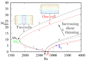
  $L=0.1$ has strongly evolved. The two primary bifurcations have changed from supercritical to subcritical, with an already important subcriticity. Both subcritical branches $B_1$ and $B_2$ turn towards larger ${Ra}$ values at saddle-node points $SN_1$ (black solid square, ${Ra}_{SN_1}=1788.96$) and $SN_2$ (green solid square, ${Ra}_{SN_2}=1822.42$), respectively. For $L=0.1$, as the first primary branch $B_1$ emerges subcritically, it is now one-time unstable at onset and is stabilized beyond the saddle-node point $SN_1$. Conversely, the second primary branch $B_2$ is now two-time unstable at onset, becomes one-time unstable at the secondary bifurcation point $S_2$ and is eventually stabilized beyond the saddle-node point $SN_2$. For such sufficiently large values of $L$, the important bifurcation points are then the saddle-node points $SN_1$ and $SN_2$ as, for both primary branches, they determine the range of ${Ra}$ where stable flow solutions can be obtained.

Figure 4. Bifurcation diagrams in the case of a shear-thinning fluid with  $n=0.5$ for three different values of $L$, 0, 0.01 and 0.1. First branch $B_1$ initiated at $P_1$ in black, second branch $B_2$ initiated at $P_2$ in red. The branches in the Newtonian case ( $L=0$) are given as dashed lines. The number of unstable real eigenvalues is indicated for each branch, $0$ corresponding to the stable solutions. The secondary bifurcation $S_2$ on the $B_2$ branch is given as blue solid circles. Saddle-node bifurcations appear on both branches for $L=0.1$.
To get a better understanding of the change of the bifurcation diagram with  $L$, we separately give the evolutions of the two branches $B_1$ and $B_2$ in figures 5 and 6. Different values of $L$ have been chosen between 0 and 1 for which the branches have been followed up to ${Ra}=5000$. Note that, for the larger values of $L$, the calculation has been stopped earlier, as soon as the convergence of the solutions by the Newton method becomes lengthy (due to the increasing importance of the viscous terms that are considered as explicit in the Newton steps), but in any case beyond the saddle-node point. In both cases, we have also followed the path of the different bifurcation points by continuation, $SN_1$ for $B_1$ and $SN_2$ and $S_2$ for $B_2$.

Figure 5. Modification of the first primary branch  $B_1$ of the bifurcation diagram in the case of a shear-thinning fluid with $n=0.5$ for an increase of $L$ from 0 to 1 (0, 0.01, 0.02, 0.03, 0.04, 0.06, 0.1, 0.2, 0.3, 0.5, 0.8, 1). The branch in the Newtonian case ( $L=0$) is given as a dashed line. The path of the saddle-node point $SN_1$ (black solid squares) is also given.

Figure 6. Modification of the second primary branch  $B_2$ of the bifurcation diagram in the case of a shear-thinning fluid with $n=0.5$ for an increase of $L$ from 0 to 1 (0, 0.01, 0.02, 0.03, 0.04, 0.06, 0.1, 0.2, 0.3, 0.5, 0.8, 1). The branch in the Newtonian case ( $L=0$) is given as a dashed line. The paths of the secondary bifurcation point $S_2$ (blue solid circles) and saddle-node point $SN_2$ (green solid squares) are also given.
The change of the first branch  $B_1$ with $L$ is shown in figure 5. We see that the saddle-node point $SN_1$ does not exist for $L=0.02$, whereas it is present for $L=0.03$, indicating that it appears between these values. A more precise estimation of this limit value $L_{l,SN_1}$ can be obtained by following the path of $SN_1$ by continuation. We thus get $L_{l,SN_1}\approx 0.0278$. The $B_1$ branch will then evolve supercritically for values of $L$ below $L_{l,SN_1}$ and subcritically for values of $L$ above $L_{l,SN_1}$. Note that, for the larger values of $L$, the subcritical part of $B_1$ appears at $P_1$ with a very weak flow intensity, and that the range of such solutions with weak flows increases with $L$. Concerning the evolution of $SN_1$, we see that $|u|_{max}$ associated with $SN_1$ progresses quickly close above the limit value $L_{l,SN_1}$ at almost constant ${Ra}$. Its critical value ${Ra}_{SN_1}$ is then found to decrease with the increase of $L$, reaching the value 610.15 for $L=1$. In a similar way, the change of the second branch $B_2$ with $L$ is shown in figure 6. The subcritical character of $B_2$ still appears above a limit value of $L$ which can be estimated at $L_{l,SN_2}\approx 0.0263$. Above this value, the saddle-node $SN_2$ exists and its critical value ${Ra}_{SN_2}$ is also found to decrease with the increase of $L$, reaching the value 604.01 for $L=1$, a value even slightly smaller than for $SN_1$. Concerning the secondary bifurcation $S_2$, its threshold ${Ra}_{S_2}$ decreases with the increase of $L$, from values above ${Ra}_{P_2}$ to values below ${Ra}_{P_2}$, $S_2$ being thus located in the subcritical part of the branch. For large $L$, due to the weak flows in these subcritical parts of $B_2$, $S_2$ is associated with small values of $|u|_{max}$ and its threshold ${Ra}_{S_2}$ seems to tend towards a constant.
3.4.2. Paths of the bifurcation points
As the different bifurcation points play a crucial role in the flow dynamics, determining in particular the domains of existence of the stable solutions, it is interesting to follow their paths more precisely and plot their characteristics as a function of  $L$. For the three bifurcation points $SN_1$, $SN_2$ and $S_2$, we give $|u|_{max}$, ${Nu}-1$ and ${Ra}_c$ vs $L$ in figure 7(a–c). In figure 7(a), we see the very steep increase of $|u|_{max}$ at the onset of the saddle-node points $SN_1$ and $SN_2$, before a moderate decrease for larger values of $L$. A similar trend is found for the Nusselt number, with a still weaker final decrease. The onsets of $SN_1$ and $SN_2$ can be determined from their paths calculated for decreasing values of $L$. We find that $SN_1$ appears on the first branch $B_1$ for $L_{l,SN_1}\approx 0.0278$ at ${{Ra}_c}\approx 2725.5$, i.e. very close to the primary threshold ${{Ra}}_{P_1}=2726.53$, whereas $SN_2$ appears on the second branch $B_2$ for $L_{l,SN_2}\approx 0.0263$ at ${{Ra}_c}\approx 2818.4$, i.e. also very close to the primary threshold ${{Ra}}_{P_2}=2818.78$. Considering these very steep variations and the difficulty of following bifurcation points in such conditions, it can be expected that the curves of $SN_1$ and $SN_2$ in figure 7(a) will in fact go to $|u|_{max}=0$ (and in figure 7(b) to ${Nu}-1=0$) for $L$ values very close to $L_{l,SN_1}$ and $L_{l,SN_2}$, respectively, and that the saddle-node points $SN_1$ and $SN_2$ emerge in reality directly from the primary bifurcations $P_1$ and $P_2$ of their respective branch. If the curves of $SN_1$ and $SN_2$ are quite distinct in terms of $|u|_{max}$ and ${Nu}-1$, they are in contrast very close in terms of ${Ra}_c$ (figure 7c), except, indeed, at their onsets, where they are close to ${{Ra}}_{P_1}$ and ${{Ra}}_{P_2}$, respectively. This means that, when shear-thinning properties are involved, the onset of the stable solutions at the saddle nodes does not depend much on the type of flow considered, two transverse rolls on $B_1$ and one longitudinal roll on $B_2$. Concerning the secondary bifurcation point $S_2$, its characteristics (threshold ${Ra}_c$, flow intensity $|u|_{max}$ and Nusselt number ${Nu}-1$) decrease with the increase of $L$, the main variations occurring for $L <0.2$. For larger $L$,
$L$,  $|u|_{max}$ and ${Nu}-1$ slowly diminish to very small values, whereas ${Ra}_c$ tends towards a limit value at ${Ra}_{l,S_2}\approx 2317$, as already expected from figure 6.

Figure 7. For a shear-thinning fluid with  $n=0.5$, paths of the different bifurcation points $SN_1$ (black dashed lines), $SN_2$ (green solid lines) and $S_2$ (blue solid lines) as a function of $L$, expressed through the variation of $|u|_{max}$ in (a), ${Nu}-1$ in (b) and ${Ra}_c$ in (c). On the first branch, $SN_1$ appears for $L_{l,SN_1}\approx 0.0278$ at ${{Ra}_c}\approx 2725.5$. On the second branch, $SN_2$ appears for $L_{l,SN_2}\approx 0.0263$ at ${{Ra}_c}\approx 2818.4$.
Finally, the different curves in figure 7 and their crossings give information about the modification of the stable parts of the two branches  $B_1$ and $B_2$ when $L$ is increased. For small $L$ and until $L=L_{l,SN_1}\approx 0.0278$, $B_1$ is stable above the primary bifurcation point $P_1$ (constant threshold at ${{Ra}}_{P_1}=2726.53$). For $L$ values beyond $L_{l,SN_1}$, $B_1$ will become stable above the saddle-node bifurcation $SN_1$ (decreasing threshold given by the black dashed curve in figure 7c). Concerning $B_2$, it is first stable for small $L$ above the secondary bifurcation $S_2$ (decreasing threshold given by the blue solid curve in figure 7c), and then, after the crossing of the $S_2$ and $SN_2$ curves at $L \approx 0.0298$, it becomes stable above the saddle node bifurcation $SN_2$ (decreasing threshold given by the green solid curve in figure 7c).
3.4.3. Change of the flow characteristics
We analyse the change of the flow characteristics at a fixed  ${Ra}$ ( ${Ra}=5000$) for a shear-thinning fluid with $n=0.5$, when the parameter $L$ is increased from 0 to 0.1. The maximum absolute values of the vertical velocity and the Nusselt number for both stable flows on branches $B_1$ and $B_2$ are given as a function of $L$ in figure 8. The curves of velocity (figure 8a) are very similar for both branches (with a parallel evolution, the curve for the branch $B_1$ remaining above) and they correspond to an increase of $|u_{max}|$ with $L$. The increase is weak close to $L=0$ (horizontal tangent), but progresses then quickly with a maximum slope of the curve for $L$ of approximately 0.024. Beyond this value, the increase becomes less steep, with a slope slowly varying in the vicinity of $L=0.1$. The curves of ${Nu}-1$ (figure 8b) increase in a similar way as the velocity curves. Note that the curve increases slightly more quickly for the branch $B_1$ than for the branch $B_2$, inducing an increased difference between them when $L$ is increased.

Figure 8. For a shear-thinning fluid with  $n=0.5$ (increasing curves) and a shear-thickening fluid with $n=1.5$ (decreasing curves), change of $|u|_{max}$ (a) and ${Nu}-1$ (b) with $L$ for the flow solutions on the branches $B_1$ (black) and $B_2$ (red) at ${{Ra}} = 5000$.
Contours of the vertical velocity and of the viscosity are given for both flow configurations on branches  $B_1$ and $B_2$ in figures 9 and 10. Two values of $L$ are chosen, $L=0.01$ for which the flow, although increased in intensity, has a similar structure as in the Newtonian case, and $L=0.1$ for which the change of the viscosity has remarkable effects. On branch $B_1$, the flow corresponds to a two transverse rolls structure, which, in figure 9, is up along the endwalls and down in the central part of the cavity. In addition to the increase of the flow intensity, the change of $L$ from 0.01 to 0.1 induces the development of boundary layers along the walls of the cavity. For the vertical velocity $u$ plotted here, these boundary layers are visible along all the vertical boundaries. The maxima of the velocity also appear to occur closer to the walls. All these changes are connected with the change of the viscosity. The viscosity $\mu _c/\mu _0=1+\mu$, plotted in figure 9, is 1 in the Newtonian case and already decreases below 0.74 in some boundary layers for $L=0.01$, while values close to 1 remain in the core. Such viscosity becomes very small (below 0.15) in the boundary layers for $L=0.1$ and the core is also affected, with values in the range $[0.3,0.8]$ and more specifically below 0.45 in the zone at the interface of the two counter-rotating rolls. Similar observations can be made for the one longitudinal roll flow structure on the $B_2$ branch when $L$ is increased from $0.01$ to $0.1$ (figure 10): increase of the flow intensity with maxima closer to the vertical walls, development of thin boundary layers along the walls, in zones where the viscosity is found to decrease strongly. The main difference from the $B_1$ branch is that there is no zone of lower viscosity in the core because of the single roll flow structure of branch $B_2$. The plots of the viscosity in the vertical transverse midplane in figure 10 (cross-section of the longitudinal roll) clearly show the zones of smaller viscosity along the four walls, with values smaller than 0.15 for $L=0.1$. Such lower viscosity zones are visible in figure 20(a) of Bouteraa et al. (Reference Bouteraa, Nouar, Plaut, Metivier and Kalck2015), but only along the upper and lower walls, as the other boundaries are periodic boundaries. In contrast, the zones of stronger viscosity appear in the corners of the cavity and in the core of the roll. Interestingly, the maxima in the core principally occur in four places, each one being closer to one of the walls, similarly to what can be seen in figure 13 of Jenny et al. (Reference Jenny, Plaut and Briard2015) along the upper and lower no-slip walls.

Figure 9. Stable solution on the first branch  $B_1$ at ${Ra}=5000$ for two values of $L$, 0.01 and 0.1 for a shear-thinning fluid with $n=0.5$. Different contours in the horizontal midplane are shown. The flow is given by the vertical velocity $u$ and the viscosity by its normalized value corresponding to $\mu _c/\mu _0=1+\mu$ (this value is 1 in the Newtonian case).

Figure 10. Stable solution on the second branch  $B_2$ at ${Ra}=5000$ for two values of $L$, 0.01 and 0.1 for a shear-thinning fluid with $n=0.5$. Different contours in characteristic planes are shown. The flow is given by the vertical velocity $u$ and the viscosity by its normalized value corresponding to $\mu _c/\mu _0=1+\mu$ (this value is 1 in the Newtonian case).
Some more precise profiles of velocity and viscosity are given for the flow on branch  $B_2$ along the horizontal transverse $y$-axis ( $x=0$, $z=0$) in figure 11. We see the strong increase of the flow when $L$ is increased from 0 to 0.1, together with the shift of the velocity maxima towards the walls at $y=-0.5$ and $y=0.5$ determining smaller boundary layers. Concerning the viscosity, at $L=0.01$, we get decreased values (down to below 0.7) along the walls in the sheared boundary layers while the core remains close to 1, with a slight minimum at the centre connected with the shear at the centre of the roll. When $L$ is increased, the minimum values of viscosity along the walls strongly decrease and the core becomes affected by a significant decrease of the viscosity. In this zone, for the larger values of $L$ (
$L$ ( $L=0.06$ and 0.1), besides the minimum at the centre, minima are also found closer to the velocity peaks.

Figure 11. Profiles of vertical velocity  $u$ and viscosity $\mu _c/\mu _0=1+\mu$ along the transverse direction $y$ at mid-height and mid-length ( $x=0$, $z=0$) for solutions on the second branch $B_2$ at ${Ra}=5000$ for different values of $L$ (0, 0.01, 0.02, 0.03, 0.04, 0.06, 0.1) for a shear-thinning fluid with $n=0.5$ (the viscosity is 1 for $L=0$). The velocity increases when $L$ is increased, whereas the viscosity decreases.
The shape of the viscosity profiles obtained in figure 11(b) can be related to the velocity profiles plotted in figure 11(a). Indeed, for the smallest value of  $L$ (
$L$ ( $L=0.01$), only the stronger velocity gradients along the walls have an effect and decrease the viscosity in these zones. When $L$ is further increased ( $L=0.02$, 0.03, 0.04), both gradients along the walls and near the centre (around $y=0$) have an effect on the viscosity, so that minima of viscosity are found along the walls and at the centre. For still larger values of $L$ (
$L$ ( $L=0.06$, 0.1), there is a change in the velocity gradients: instead of decreasing from the value at the centre towards zero at the velocity peak, they now increase beyond about $|y|>0.2$ above the value at the centre, before decreasing to zero at the velocity peak, which creates the new viscosity minimum just below $|y|=0.3$.
As the viscosity in the Carreau model is connected with the shear rate, it is interesting to consider the shear rate in the cavity. For the branch  $B_2$, we give shear rate and shear stress norms contours in the vertical transverse midplane (cross-section of the longitudinal roll) and along the wall at $y=0.5$ for the flows at $L=0.01$ and 0.1 in figure 12, together with profiles along the horizontal transverse $y$-axis in figure 13. As expected, the shear rate $|\dot {\gamma }_{\boldsymbol u}|$ is particularly important along the walls and, in these zones, it increases strongly with $L$, from maximum values just above 200 for $L=0.01$ to maximum values beyond 1200 for $L=0.1$, whereas it remains rather weak (between 10 and 40) in the core of the cavity for the different values of $L$. In contrast, the shear stress $(\mu _c/\mu _0)|\dot {\gamma }_{\boldsymbol u}|$ evolves in the same range for the different values of $L$. This is due to the fact that the stronger values of $|\dot {\gamma }_{\boldsymbol u}|$ along the boundaries for the strongest values of $L$ are multiplied by lower values of the viscosity $(\mu _c/\mu _0)$. The shear stress reaches even smaller maximum values along the boundaries for $L=0.1$ than for $L=0.01$. Despite the small variations of the shear stress with $L$, the profiles presented in figure 13(b) evolve with $L$ due to the thinner boundary layers obtained when $L$ is increased. Note finally that the contours of viscosity in the vertical transverse midplane (figure 10) reproduce quite well those of the shear rate and shear stress (figure 12).

Figure 12. Isocontours in different planes for the shear rate  $|\dot {\gamma }_{\boldsymbol u}|$ (a–b,e–f) and shear stress $(\mu _c/\mu _0)|\dot {\gamma }_{\boldsymbol u}|$ (c–d,g–h) for a stable solution on the second branch $B_2$ at ${Ra}=5000$ for a shear-thinning fluid with $n=0.5$, $L=0.01$ or $L=0.1$. The norms of these fields are given in the vertical transverse midplane and along the lateral wall at $y=0.5$.

Figure 13. Profiles of shear rate  $|\dot {\gamma }_{\boldsymbol u}|$ (a) and shear stress $(\mu _c/\mu _0)|\dot {\gamma }_{\boldsymbol u}|$ (b) along the transverse direction $y$ at mid-height and mid-length ( $x=0$, $z=0$) for solutions on the second branch $B_2$ at ${Ra}=5000$ for different values of $L$ (0.01, 0.02, 0.03, 0.04, 0.06, 0.1) for a shear-thinning fluid with $n=0.5$. The shear rate increases on the boundaries when $L$ is increased, whereas the shear stress does not change much.
3.4.4. Order of magnitude analysis of the subcritical convection onset
For this order of magnitude analysis, we come back to a very simplified 2-D inertialess approach, in a plane perpendicular to the rolls axis. We will use a dimensionless formulation as that given by (2.6), (2.8) and (2.9). A common idea is that rolls are observed when the heat diffusion time across the domain,  $\tau _{diff} \approx 1/{\rm \pi} ^2$, is equivalent to the heat convection time when rolls are present, $\tau _{conv} \approx 1/u$, where $u$ is a vertical velocity. The characteristic speed of the rolls at onset at the saddle-node point can then be estimated as $u_{SN} \approx {\rm \pi}^2$, which is consistent with what is observed for $n=0.5$ in figures 5 and 6.
To get an order of magnitude expression for the velocity, we first eliminate the pressure in (2.8) by taking the curl of this equation. In a steady inertialess approach, we get
 \begin{equation} \boldsymbol{\nabla} \times (\boldsymbol{\nabla} \boldsymbol{\cdot} ((1+\mu) \dot{\gamma}_{\boldsymbol u})) + {Ra} \, \boldsymbol{\nabla} \times ( T {\boldsymbol e_x}) =0. \end{equation}
Between two rolls, in the middle plane of the cavity, the order of magnitude of the first (viscous) term, denoted as  $Q_{visc}$, can be obtained by focusing on the horizontal variations (considered along $z$) of the vertical velocity (along $x$)
$x$)
 \begin{equation} Q_{visc}=\boldsymbol{\nabla} \times (\boldsymbol{\nabla} \boldsymbol{\cdot} ((1+\mu) \dot{\gamma}_{\boldsymbol u})) \approx \frac{\partial^2}{\partial z^2} \left((1+\mu) \frac{\partial u}{\partial z}\right). \end{equation}
An additional assumption is that the subcritical onset corresponds to a strong enough convective state for the fluid to behave as a power-law fluid ( $\dot {\gamma }_{\boldsymbol u} \gg L$, see figure 14(b) for an estimate of $\dot {\gamma }_{\boldsymbol u}$ justifying this assumption). Using (2.6), we can then write
 \begin{equation} (1+\mu) = [1+(L |\dot{\gamma}_{\boldsymbol u}|)^2]^{(n-1)/2} \approx (L |\dot{\gamma}_{\boldsymbol u}|)^{n-1} \approx \left(L |\frac{\partial u}{\partial z}|\right)^{n-1}. \end{equation}
Then  $Q_{visc}$ can be estimated as
 \begin{equation} Q_{visc} \approx \frac{\partial^2}{\partial z^2} \left(\left(L \left|\frac{\partial u}{\partial z}\right|\right)^{n-1} \frac{\partial u}{\partial z}\right) \approx L^{n-1} \frac{{u_{SN}}^n}{\xi^{n+2}} \approx \frac{{\rm \pi}^{2n}}{\xi^{n+2}} L^{n-1}, \end{equation}
where a flow shape factor  $\xi$ has been introduced to account for several effects enhancing dissipation in the system (size of the rolls smaller than 1, shear due to the sidewalls); $\xi$ is expected to be smaller than one and to depend on the power-law index $n$ of the Carreau model. Concerning the buoyant term in (3.1), denoted as $Q_{buoy}$, it can be estimated as
 \begin{equation} Q_{buoy} = {Ra} \, \boldsymbol{\nabla} \times ( T {\boldsymbol e_x}) = {Ra} \, \frac{\partial T}{\partial z} \approx \frac{{Ra}}{2}, \end{equation}
if we assume a horizontal temperature gradient between the rolls  $\partial T/\partial z \approx \frac {1}{2}$. From the balance of the viscous and buoyant terms given by (3.1), an estimation of the subcritical Rayleigh number ${Ra}_{SN}$ can finally be obtained
 \begin{equation} {Ra}_{SN} \approx 2 {\rm \pi}^{2n} \left(\frac{1}{\xi(n)}\right)^{n+2} L^{n-1}. \end{equation}
Let us recall that this very crude approach is known, when applied to the Rayleigh–Bénard problem featuring a Newtonian fluid, to underestimate the threshold value for the onset of convection, though it provides a practical interpretation for the expression of the Rayleigh number. Here, choosing  $n=1$, we recover the approximated value for the Newtonian case.

Figure 14. Variation of the critical Rayleigh number  ${Ra}_c$ (a) and of the maximum shear rate $|\dot {\gamma }_{\boldsymbol u}|$ (b) for the saddle-node point on the first branch as a function of $L$ for a shear-thinning fluid with different values of $n$. In (a), the numerically obtained variations of ${Ra}_{SN_1}$ with $L$ (black solid lines) are compared with different approximations: ${Ra}_{SN_1}|_{L=1} L^{n-1}$ ( $L^{n-1}$ variation given by the model, adjusted with the data for $L=1$) (red dashed lines); $Ra_{P_1} n^{2.25} L^{n-1}$ (3.7) (green dashed lines).
In figure 14, for the saddle-node point on the branch  $B_1$, we present the variation of the critical Rayleigh number ${Ra}_{SN_1}$ and of the maximum shear rate $|\dot {\gamma }_{\boldsymbol u}|$ as a function of $L$ for different values of the power-law index $n$. In figure 14(a), we have first compared the curves giving the critical value of ${Ra}$ (black solid lines) with the $L^{n-1}$ variation given by the order of magnitude analysis by adjusting the curves at $L=1$ for each value of $n$ (red dashed lines). We see that ${Ra}_{SN_1}$ depends on $n$, but varies quite well as $L^{n-1}$ at fixed value of $n$. In a 2-D periodic cavity, Jenny et al. (Reference Jenny, Plaut and Briard2015) also obtained a close to $L^{n-1}$ variation by fitting their data by a power-law behaviour. The subsequent dependence on $n$ of their data was then well fitted by a power of $n$, precisely $n^{2.2411}$, the multiplicative constant being close to the Newtonian threshold. Note also that for a shear-thinning fluid described by a power-law model (Turan et al. Reference Turan, Fotso-Choupe, Lai, Poole and Chakraborty2014), the minimum ${Ra}$ for 2-D convection to occur was also expressed as a function of the power-law index $n$ by characteristic laws, ${Ra}^{Newt}_c n^{2.5}$ and ${Ra}^{Newt}_c n^{2}$ (where ${Ra}^{Newt}_c$ is the Newtonian value), for prescribed temperature and prescribed flux at the horizontal boundaries, respectively. Following these ideas to fit the variations with a power of $n$ with a prefactor equal to the Newtonian threshold, we also plot the curves ${Ra}_{P_1} n^{2.25} L^{n-1}$ (green dashed lines) in figure 14(a). We see that the fit is not perfect, indicating that the proposed expression is too simple to perfectly catch the observed variations. This law, however, gives a reasonable estimation of the threshold variation for $SN_1$, except closer to the limit $L_{l,SN_1}$ where clearly overestimated values will be obtained compared with the expected ${Ra}_{P_1}$ value. We verified that the proposed law also fitted well the data for the saddle-node $SN_2$ on branch $B_2$. We then got the following approximate expressions for the saddle-node critical Rayleigh numbers:
 \begin{equation} {Ra}_{SN_1} \approx {Ra}_{P_1} n^{2.25} L^{n-1}, \end{equation}
and
 \begin{equation} {Ra}_{SN_2} \approx {Ra}_{P_2} n^{2.25} L^{n-1}. \end{equation}
Concerning the shear rate, the order of magnitude analysis simply gives
 \begin{equation} \dot{\gamma}_{\boldsymbol u} \approx \frac{\partial u}{\partial z} \approx \frac{u_{SN}}{\xi(n)} \approx \frac{{\rm \pi}^2}{\xi(n)}. \end{equation}
In figure 14(b), we see that the maximum shear rate quickly tends to a constant when  $L$ is increased and that this constant strongly depends on $n$, changing from 40 for $n=0.9$ to approximately 230 for $n=0.5$. Interestingly, the expression (3.9) obtained with the model gives a shear rate which does not depend explicitly on $L$, featuring the constant values reached by the data in figure 14(b). Moreover, assuming as previously that $\xi$ depends on $n$ and takes values smaller than 1, this shear rate is expected to reach values of several dozen, in agreement with the data.
3.4.5. Perturbation kinetic energy budgets at the transitions
Some information at the flow transitions can be obtained from the calculation at threshold of the perturbation kinetic energy budget associated with the perturbations (critical eigenvector). The basic steady solution at threshold [ $u_i$, $T$](
$T$]( $x_i$) and the critical eigenvector [ $u_{p,i}$, $T_p$]( $x_i$) both enter the equation of energy budget giving the rate of change of the perturbation kinetic energy defined as $e_k={\mathcal {R}}e(u_{p,i} \bar {u}_{p,i} /2)$ ( ${\mathcal {R}}e$ and the overbar denote the real part and the complex conjugate, respectively). After integration on the volume of the cavity, an equation for the rate of change of the total perturbation kinetic energy ( $E_k= \int _{\varOmega } e_k \, \textrm {d}\varOmega$) can be obtained
 \begin{equation} \frac{\partial E_k}{\partial t} = E_{shear} + E_{buoy} + E_{visc,0} + E_{visc,c} + E_{visc,p} ,\end{equation}
where
 \begin{gather} E_{shear}= {\mathcal{R}}e \left (- \int_{\varOmega} u_{p,j} \frac{\partial u_i}{\partial x_j} \bar{u}_{p,i} \, {\rm d}\varOmega \right ), \end{gather}
 \begin{gather}E_{buoy}= {\mathcal{R}}e \left ({Pr} \, {Ra} \int_{\varOmega} T_p \bar{u}_{p,i} \delta_{i1} \, {\rm d}\varOmega\right ), \end{gather}
 \begin{gather}E_{visc,0}= {\mathcal{R}}e \left (- {Pr} \int_{\varOmega} \frac{\partial u_{p,i}}{\partial x_j} \frac{\partial \bar{u}_{p,i}}{\partial x_j} \, {\rm d}\varOmega \right ), \end{gather}
 \begin{gather}E_{visc,c}= {\mathcal{R}}e \left (- {Pr} \int_{\varOmega} \mu \dot{\gamma}_{ \boldsymbol u_p ,ij} \frac{\partial \bar{u}_{p,i}}{\partial x_j} \, {\rm d}\varOmega \right ), \end{gather}
 \begin{gather}E_{visc,p}= {\mathcal{R}}e \left (- {Pr} \int_{\varOmega} (\partial \mu/\partial \boldsymbol u){ \boldsymbol u_p} \dot{\gamma}_{\boldsymbol u ,ij} \frac{\partial \bar{u}_{p,i}}{\partial x_j} \, {\rm d}\varOmega \right ). \end{gather}
Here,  $E_{shear}$ represents the production of perturbation kinetic energy by shear of the basic flow (inertia term), $E_{buoy}$ the production of perturbation kinetic energy by buoyancy, $E_{visc,0}$ the viscous dissipation of perturbation kinetic energy associated with the Newtonian viscosity, $E_{visc,c}$ the viscous contribution associated with the extra Carreau viscosity $\mu$ and $E_{visc,p}$ the viscous contribution associated with the perturbation of the Carreau viscosity. At threshold, the critical eigenvector is associated with an eigenvalue with zero real part. This implies that ${\partial E_k / \partial t}$ is equal to zero at marginal stability. Finally, we normalize (3.10) by $-E_{visc,0}=|E_{visc,0}|$, which is always positive, to get an equation involving normalized energy terms $E'=E/|E_{visc,0}|$ at threshold
 \begin{equation} E'_{shear} + E'_{buoy} + E'_{visc,c} + E'_{visc,p} =1. \end{equation}
 Finally, the critical Rayleigh number can also be expressed as a function of energetic contributions. For that, we use the fact that the expression of  $E'_{buoy}$ linearly depends on ${Ra}$. At the threshold, we can write $E'_{buoy} = {Ra}_c E''_{buoy}$. And from (3.16), we get ${Ra}_c E''_{buoy} = 1- E'_{shear} - E'_{visc,c} - E'_{visc,p}$ which, in the Newtonian case, gives ${Ra}_0 E''_{buoy,0} = 1- E'_{shear,0}$, where the subscript 0 refers to the Newtonian case. Finally, if we assume that the shear contributions remain small and can be neglected (as we will see later), the ratio of these two equations gives
 \begin{equation} \frac{{Ra}_c}{{Ra}_0} = \frac{ \overbrace{(1- E'_{visc,c} - E'_{visc,p})}^{{R_{visc}}} }{ \underbrace{ ( { E''_{buoy} / E''_{buoy,0}} ) }_{{R_{buoy}}} } , \end{equation}
which indicates that the variation of  ${Ra}_c$ with the non-Newtonian properties (as the value of $L$) can be expressed through the ratio of the two factors, $R_{visc}$ and $R_{buoy}$, the first factor being connected to the global viscous contributions and the second factor to the buoyancy contributions. Without non-Newtonian contributions, $R_{visc}$ and $R_{buoy}$ are equal to 1 and ${Ra}_c={Ra}_0$.
The different contributions to the perturbation kinetic energy expressed in (3.16) are first given as a function of  $L$ for the secondary bifurcation $S_2$ on the branch $B_2$ in figure 15(a). At $L=0$, the shear contribution $E'_{shear}$ has only a very weak destabilization effect so that the destabilization is mainly due to the buoyancy contribution $E'_{buoy}$. When $L$ is increased, this shear contribution decreases so as to become negligible, whereas the two extra viscous contributions connected with the shear-thinning properties increase and give destabilizing contributions. They, however, remain rather small (approximately 0.13 for the extra Carreau viscosity contribution $E'_{visc,c}$ and 0.03 for the contribution of the Carreau viscosity perturbation $E'_{visc,p}$) and $E'_{buoy}$ keeps the larger destabilizing values. Note that all these quantities quickly reach asymptotic values (for $L$ larger than about 0.3), as it was already observed for the threshold ${Ra}_{S_2}$ in figure 7(b). The variation of the energy factors $R_{visc}$ and $R_{buoy}$ in this case is given in figure 15(b), together with the variation of ${Ra}_c/{Ra}_0$. We observe that the decrease of the critical Rayleigh number is due to the decrease of the viscous ratio $R_{visc}$, but is accentuated by the increase of the buoyancy ratio $R_{buoy}$.

Figure 15. Perturbation kinetic energy budgets at the secondary bifurcation point  $S_2$ on the branch $B_2$ as a function of $L$ for a shear-thinning fluid with $n=0.5$. Variation of the perturbation kinetic energy terms (a). The different contributions are normalized by the viscous dissipation associated with the Newtonian viscosity: the inertia term $E'_{shear}$ (red), the buoyancy term $E'_{buoy}$ (green), the viscous contribution associated with the extra Carreau viscosity $E'_{visc,c}$ (blue) and the viscous contribution associated with the perturbation of the Carreau viscosity $E'_{visc,p}$ (pink). Energetic contributions to the critical Rayleigh number, $R_{visc}$ and $R_{buoy}$ such that ${Ra}_c/{Ra}_0=R_{visc}/R_{buoy}$ (b). The viscous factor $R_{visc}$ is given as a blue line, the buoyancy factor $R_{buoy}$ as a green line and the Rayleigh number ratio ${Ra}_c/{Ra}_0$ as a red line.
The energy contributions are also plotted for the saddle-node point  $SN_1$ in figure 16(a). The evolution of these quantities with $L$ is very similar for the two saddle-node points and very different from what was previously observed for $S_2$. As soon as the saddle-node point $SN_1$ is created at $L_{l,SN_1}$, the energy contributions evolve very quickly from their values at the primary bifurcation point $P_1$ ( $E'_{shear}=E'_{visc,c}=E'_{visc,p}=0$, $E'_{buoy}=1$). The two extra viscous contributions connected with the shear-thinning properties increase first very quickly in a similar way, but the contribution of the Carreau viscosity perturbation $E'_{visc,p}$ reaches quickly a maximum before a regular decrease, whereas the extra Carreau viscosity contribution $E'_{visc,c}$ continues to regularly increase. The shear contribution $E'_{shear}$ also increases, but remains really weak. As a consequence of (3.16), the buoyancy contribution $E'_{buoy}$ must decrease. It decreases, first very quickly and then more gently and, surprisingly, follows the decrease of $E'_{visc,p}$ in this second stage. We did not succeed in explaining this behaviour, although it does not seem to be incidental as it is observed for both saddle-node points. If we finally add the different viscous contributions, we find then that the global stabilizing viscous contribution expressed by $1-E'_{visc,c}-E'_{visc,p}$ has strongly decreased (mainly due to the extra Carreau viscosity contribution) and is equilibrated by a decreased buoyancy contribution and a weak shear contribution.

Figure 16. Perturbation kinetic energy budgets at the saddle-node point  $SN_1$ on the branch $B_1$ as a function of $L$ for a shear-thinning fluid with $n=0.5$. Variation of the perturbation kinetic energy terms (a). The different contributions are normalized by the viscous dissipation associated with the Newtonian viscosity: the inertia term $E'_{shear}$ (red), the buoyancy term $E'_{buoy}$ (green), the viscous contribution associated with the extra Carreau viscosity $E'_{visc,c}$ (blue) and the viscous contribution associated with the perturbation of the Carreau viscosity $E'_{visc,p}$ (pink). Energetic contributions to the critical Rayleigh number, $R_{visc}$ and $R_{buoy}$ such that ${Ra}_c/{Ra}_0=R_{visc}/R_{buoy}$ (b). The viscous factor $R_{visc}$ is given as a blue line, the buoyancy factor $R_{buoy}$ as a green line and the Rayleigh number ratio ${Ra}_c/{Ra}_0$ as a red line.
The variations with  $L$ of $R_{visc}$ and $R_{buoy}$ for the saddle-node point $SN_1$, together with the variations of ${Ra}_c/{Ra}_0$, are given in figure 16(b). For both saddle-node points, we observe a simultaneous strong decrease of $R_{visc}$ and $R_{buoy}$. This decrease, however, slows down more rapidly for $R_{buoy}$ than for $R_{visc}$, so that $R_{visc}$ remains smaller than $R_{buoy}$ with an increased difference between them when $L$ is increased and ${Ra}_c/{Ra}_0$, less than 1, decreases then with the increase of $L$. We can finally state that the decrease of the critical Rayleigh number for the saddle-node points $SN_1$ and $SN_2$ is a consequence of the decrease of the viscous factor $R_{visc}$ due to the shear-thinning properties of the fluid, but this effect is attenuated by the decrease of the buoyancy factor $R_{buoy}$.
3.5. Shear-thickening Carreau fluid
In this section, we will now study the influence of the shear-thickening properties on the bifurcation diagram. We choose a power-law index  $n=1.5$ and vary the parameter $L$. As indicated in § 3.4, the primary thresholds are not modified by the non-Newtonian properties and are the same as in the Newtonian case.
3.5.1. Bifurcation diagrams
The change of the bifurcation diagram with  $L$ for a shear-thickening fluid is illustrated by the evolution of the two branches $B_1$ and $B_2$ in figure 17. Different values of $L$ have been chosen between 0 and 0.1 for which the branches have been followed up to ${Ra}=5000$. Both branches keep evolving supercritically when $L$ is increased, but correspond to weaker flow intensities. Such decrease of the flow intensity for a shear-thickening fluid is depicted in figure 8 where the variation of $|u_{max}|$ with $L$ at ${Ra}=5000$ is given for both branches. For the branch $B_2$, we have also followed the path of the secondary bifurcation point $S_2$ by continuation when increasing $L$. In figure 17(b), we see the quick displacement of $S_2$, even for small values of $L$. More information is given in figure 18 with the plots of $|u_{max}|$ and ${Ra}_c$ as a function of $L$ for this point $S_2$. Both values increase with $L$, but the major fact is the strong increase of ${Ra}_c$ (almost linear beyond $L=0.04$), which indicates that the stabilization of the branch $B_2$ beyond $S_2$ is delayed to larger thresholds when $L$ is increased.

Figure 17. Modification of the first primary branches of the bifurcation diagram (branch  $B_1$ in a and branch $B_2$ in b) in the case of a shear-thickening fluid with $n=1.5$ for an increase of $L$ from 0 to 0.1 (0, 0.01, 0.02, 0.03, 0.05, 0.1). The branch in the Newtonian case ( $L=0$) is given as a dashed line. The path of the secondary bifurcation point $S_2$ (blue solid circles) is also given in (b).

Figure 18. For a shear-thickening fluid with  $n=1.5$, paths of the bifurcation point $S_2$ as a function of $L$, expressed through the variation of $|u|_{max}$ in (a) and ${Ra}_c$ in (b).
3.5.2. Change of the flow characteristics
Contours of the vertical velocity and of the viscosity are given for both branches  $B_1$ and $B_2$ for a shear-thickening fluid with $n=1.5$ in figures 19 and 20 for ${Ra}=5000$ and two values of $L$, 0.01 and 0.1. The profiles along the horizontal transverse $y$-axis are also given for $B_2$ for different values of $L$ in figure 21. The change of the flow structure is less marked than for shear-thinning fluids. The increased viscosity along the boundaries, which can reach values up to 2, slows down the flows, but does not change the flow structure much, except that the maximum vertical velocity occurs slightly farther from the boundaries. Profiles of shear stress and shear rate are also presented in figure 22. The shear rate $|\dot {\gamma }_{\boldsymbol u}|$ decreases with the increase of $L$, from maximum values along the walls above 100 for $L=0.01$ to 40 for $L=0.1$. This moderate decrease is connected with the moderate increase of the viscosity, which is due to the fact that the expected change of viscosity related to the change of $L$ (2.4) is attenuated by the decrease of $|\dot {\gamma }_{\boldsymbol u}|$ due to the decreased flow intensity. As expected, the shear stress $(\mu _c/\mu _0)|\dot {\gamma }_{\boldsymbol u}|$ is still less contrasted between the two values of $L$, due to the fact that the smaller values of $|\dot {\gamma }_{\boldsymbol u}|$ obtained along the boundaries for the larger values of $L$ are multiplied by larger values of the viscosity $(\mu _c/\mu _0)$.

Figure 19. Stable solution on the first branch  $B_1$ at ${Ra}=5000$ for a shear-thickening fluid with $n=1.5$ and two values of $L$, 0.01 and 0.1. Different contours in the horizontal midplane are shown. The flow is given by the vertical velocity $u$ and the viscosity by its normalized value corresponding to $\mu _c/\mu _0=1+\mu$ (this value is 1 in the Newtonian case).

Figure 20. Stable solution on the second branch  $B_2$ at ${Ra}=5000$ for a shear-thickening fluid with $n=1.5$ and two values of $L$, 0.01 and 0.1. Different contours in the horizontal midplane are shown. The flow is given by the vertical velocity $u$ and the viscosity by its normalized value corresponding to $\mu _c/\mu _0=1+\mu$ (this value is 1 in the Newtonian case).

Figure 21. Profiles of vertical velocity  $u$ (a) and viscosity $\mu _c/\mu _0=1+\mu$ (b) along the transverse direction $y$ at mid-height and mid-length ( $x=0$, $z=0$) for solutions on the second branch $B_2$ at ${Ra}=5000$ for a shear-thickening fluid with $n=1.5$ and different values of $L$ (0, 0.01, 0.02, 0.03, 0.05, 0.1) (the viscosity is 1 for $L=0$). The velocity decreases when $L$ is increased, whereas the viscosity increases.

Figure 22. Profiles of shear rate  $|\dot {\gamma }_{\boldsymbol u}|$ (a) and shear stress $(\mu _c/\mu _0)|\dot {\gamma }_{\boldsymbol u}|$ (b) along the transverse direction $y$ at mid-height and mid-length ( $x=0$, $z=0$) for solutions on the second branch $B_2$ at ${Ra}=5000$ for a shear-thickening fluid with $n=1.5$ and different values of $L$ (0.01, 0.02, 0.03, 0.05, 0.1). The shear rate and shear stress decrease when $L$ is increased.
3.5.3. Perturbation kinetic energy budgets at  $S_2$
$S_2$

The different contributions to the perturbation kinetic energy expressed in (3.16) are given as a function of  $L$ for the secondary bifurcation $S_2$ on the branch $B_2$ in figure 23(a). The shear contribution $E'_{shear}$ with a very weak destabilization remains negligible. The destabilization is due to the buoyancy contribution $E'_{buoy}$, which increases when $L$ is increased, in connection with the increased stabilizing extra viscous contributions. Here also the extra Carreau viscosity contribution $E'_{visc,c}$ is really larger than the contribution of the Carreau viscosity perturbation $E'_{visc,p}$. The variation of the energy factors $R_{visc}$ and $R_{buoy}$ in this case is given in figure 23(b), together with the variation of ${Ra}_c/{Ra}_0$. We observe that the strong increase of the critical Rayleigh number is due to the increase of the viscous ratio $R_{visc}$, but is accentuated by the decrease of the buoyancy ratio $R_{buoy}$, in connection with the change of the perturbation structure.

Figure 23. Perturbation kinetic energy budgets at the secondary bifurcation point  $S_2$ on the branch $B_2$ as a function of $L$ for a shear-thickening fluid with $n=1.5$. Variation of the perturbation kinetic energy terms (a). The different contributions are normalized by the viscous dissipation associated with the Newtonian viscosity: the inertia term $E'_{shear}$ (red), the buoyancy term $E'_{buoy}$ (green), the viscous contribution associated with the extra Carreau viscosity $E'_{visc,c}$ (blue) and the viscous contribution associated with the perturbation of the Carreau viscosity $E'_{visc,p}$ (pink). Energetic contributions to the critical Rayleigh number, $R_{visc}$ and $R_{buoy}$ such that ${Ra}_c/{Ra}_0=R_{visc}/R_{buoy}$ (b). The viscous factor $R_{visc}$ is given as a blue line, the buoyancy factor $R_{buoy}$ as a green line and the Rayleigh number ratio ${Ra}_c/{Ra}_0$ as a red line.
3.6. Influence of the Prandtl number
As shear-thinning fluids may have high Prandtl number values, we want to quantify the influence of an increase of the Prandtl number  ${Pr}$ on our results. For that, we consider the critical Rayleigh number at the saddle-node point $SN_1$ for $n=0.5$ and follow its variation by continuation when ${Pr}$ is increased from 1 to 10. The results are shown in figure 24 for two values of $L$, 0.1 and 1. We see that there is a clear influence of ${Pr}$ on ${Ra}_{SN_1}$ when ${Pr}$ is increased above 1, with a first steep decrease and then a slower evolution leading to an asymptotic regime, which is already well approached for ${Pr}=10$. However, looking to the scales which are on the right side of the figure for $L=1$ and on the left side for $L=0.1$, we see that the variations remain moderate. For $L=0.1$, ${Ra}_{SN_1}$ is changed from 1788.96 for ${Pr}=1$ to 1749.76 for ${Pr}=10$, corresponding to a 2.2 $\%$ decrease, whereas for $L=1$, $Ra _{SN_1}$ is changed from 610.15 to 565.70, corresponding to a 7.3 $\%$ decrease. This indicates that the overall description of the phenomena obtained for ${Pr}=1$ remains valid for larger Prandtl numbers, with only moderate changes of the critical parameters.

Figure 24. Critical Rayleigh number at the saddle-node point  $SN_1$ as a function of the Prandtl number ${Pr}$ for $n=0.5$ and two values of $L$. The scale for the red curve ( $L=1$) is on the right side of the figure and the scale for the black curve ( $L=0.1$) is on the left side.
4. Discussion
As shown in the introduction, different authors have considered Rayleigh–Bénard convective rolls in shear-thinning fluids obeying the Carreau law, either in extended 3-D cavities by weakly nonlinear analyses (Bouteraa et al. Reference Bouteraa, Nouar, Plaut, Metivier and Kalck2015) or in 2-D cavities (Benouared et al. Reference Benouared, Mamou and Ait Messaoudene2014; Jenny et al. Reference Jenny, Plaut and Briard2015). It is interesting to compare our results concerned with rolls in a 3-D confined cavity with some of those results.
Concerning the change of the primary bifurcation to rolls from supercritical to subcritical in shear-thinning fluids, Bouteraa et al. (Reference Bouteraa, Nouar, Plaut, Metivier and Kalck2015), considering small amplitude disturbances, have shown that, for an extended cavity with upper and lower walls at fixed temperature and rigid, this change occurs at a critical value of the degree of shear-thinning parameter  $\alpha$ (2.5). For ${Pr} \geq 1$, they give $\alpha _c=2.15 \times 10^{-4}$. In order to compare with this value, for both branches $B_1$ and $B_2$ and the different values of $n$, we have looked for the value of $L$ corresponding to the limit of existence of the corresponding saddle-node point (as was done for $n=0.5$ in figure 7) and deduced the critical value of $\alpha$. The results are shown in table 3. We see that the critical value of $\alpha$ is almost constant for a given branch, i.e. a given flow structure, indicating that the shear-thinning character of the fluid is well quantified by the parameter $\alpha$ at this supercritical/subcritical transition in our 3-D cavity. More precisely, we obtain $\alpha _c \approx 1.94 \times 10^{-4}$ for the branch $B_1$ (two transverse rolls) and $\alpha _c \approx 1.73 \times 10^{-4}$ for the branch $B_2$ (one longitudinal roll). These values are a little below the critical value given by Bouteraa et al. (Reference Bouteraa, Nouar, Plaut, Metivier and Kalck2015), but really of the same order of magnitude, despite the confinement existing in our 3-D rigid cavity.
Table 3. Critical values of the rheological parameters corresponding to the transition between supercritical and subcritical behaviours for both  $B_1$ and $B_2$ branches (limit of existence of the corresponding saddle-node point). Critical values of $L$ for different power-law indexes $n$, and deduced critical values of the degree of shear-thinning parameter $\alpha$. The critical value of $\alpha$ is approximately $1.94 \times 10^{-4}$ for the branch $B_1$ and $1.73 \times 10^{-4}$ for the branch $B_2$, compared with the value $\alpha _c=2.15 \times 10^{-4}$ given for rolls in extended cavities by Bouteraa et al. (Reference Bouteraa, Nouar, Plaut, Metivier and Kalck2015).

Concerning the saddle-node points appearing on the subcritical branches in shear-thinning fluids, for a 2-D periodic square cavity Jenny et al. (Reference Jenny, Plaut and Briard2015) showed that the corresponding Nusselt number  ${Nu}$ expressed as a function of the Parmentier–Rayleigh number ${Rap}$ belongs to a single curve for any value of the shear-thinning parameters and that this curve is the ${Nu}$ vs ${Ra}$ curve obtained in the Newtonian case. We recall that the Parmentier–Rayleigh number ${Rap}$ is defined with the use of a specific volume-average viscosity, weighted by the square of the shear rate. This viscosity, called Parmentier's viscosity, is then defined, in its dimensionless form, as
 \begin{equation} \mu_p=\frac{\displaystyle\int_V (\mu_c/\mu_0) |\dot{\gamma}_{\boldsymbol u}|^2 \, {\rm d}V}{\displaystyle\int_V |\dot{\gamma}_{\boldsymbol u}|^2 \, {\rm d}V}, \end{equation}
where  $V$ denotes the volume of the cavity. For all the saddle-node points determined in our study (for the different $n$ and $L$ values and for both branches), we have calculated the Nusselt number and the Parmentier–Rayleigh number and the results expressed as ${Nu}-1$ vs ${Rap}$ are shown in figure 25, together with the primary bifurcation curves obtained for a Newtonian fluid. For each branch, there exists a master curve, clearly depicted by the green short dashed lines, but this master curve departs from the Newtonian curve and is close to it only for weakly shear-thinning fluids (values of $n$ close to 1 or small values of $L$). Moreover, for the smallest values of $n$, the data even depart from the master curves, particularly for values of $L$ above 0.1 (black and red solid lines for branches $B_1$ and $B_2$, respectively). It then seems that the collapse of the saddle-node data on a single curve, as observed by Jenny et al. (Reference Jenny, Plaut and Briard2015), is not obtained in our 3-D confined cavity. Note that this previous study (Jenny et al. Reference Jenny, Plaut and Briard2015) concerned 2-D almost square cavities with horizontal periodicity, whereas our 3-D cavity is a rigid cavity with no-slip conditions on all the boundaries, thus inducing the presence of boundary layers.

Figure 25. Reduced Nusselt number ( ${Nu}-1$) vs the Parmentier–Rayleigh number ( ${Rap}$) for the convective flows at the saddle-node points $SN_1$ and $SN_2$. All the values of $L$ up to $1$ and of $n$ (0.5, 0.6, 0.7, 0.8, 0.9) are considered. For $SN_1$, the results for each $n$ value are plotted as black solid lines for $0.1 \leq L \leq 1$, continued by green short dashed lines for $L \leq 0.1$ (down to ${Ra}_{P_1}$). For $SN_2$, the results for each $n$ value are plotted as red solid lines for $0.1 \leq L \leq 1$, continued by green short dashed lines for $L \leq 0.1$ (down to ${Ra}_{P_2}$). The primary bifurcation curves for a Newtonian fluid are given as long dashed lines, in black for branch $B_1$ and in red for branch $B_2$.
Benouared et al. (Reference Benouared, Mamou and Ait Messaoudene2014) determined the critical Rayleigh number  ${Ra}_{SN}$ for the onset of finite amplitude convection (corresponding to our saddle-node point) for a 2-D square cavity. In their Table VI, for $L=0.4$ and different values of $n$, they give the ratio of ${Ra}_{SN}$ to the linear primary threshold for a cavity with either no-slip or slip vertical walls. We give these ratios for $n=0.6$ and 0.8 in table 4, together with our corresponding results for both branches $B_1$ and $B_2$. We see that the ratios we obtain for the two branches are very close. Moreover, these ratios are also close to those obtained by Benouared et al. (Reference Benouared, Mamou and Ait Messaoudene2014), in fact located between their no-slip and slip ratios.
Table 4. For a shear-thinning fluid with  $L=0.4$ and two values of $n$ (0.6 and 0.8), values of the critical Rayleigh number at the saddle-node bifurcation and its ratio to the corresponding primary threshold for both $B_1$ and $B_2$ branches. Comparison with the ratio given by Benouared et al. (Reference Benouared, Mamou and Ait Messaoudene2014) for a 2-D square cavity with either no-slip or slip vertical walls.

Jenny et al. (Reference Jenny, Plaut and Briard2015) proposed defining different dimensionless viscosities at the saddle-node points: the Parmentier viscosity  $\mu _p$ (4.1), the bulk-average viscosity
 \begin{equation} \mu_m=\frac{\displaystyle\int_V (\mu_c/\mu_0) \, {\rm d}V}{\displaystyle\int_V {\rm d}V} \end{equation}
and an effective viscosity such that the saddle-node Rayleigh number constructed on its dimensional value is constant, equal to the Newtonian critical value. This effective viscosity, in its dimensionless form, is then defined by
 \begin{equation} \mu_e= \frac{{Ra}_{SN}}{{Ra}^{Newt}_c}, \end{equation}
which, in our case, will give  $\mu _e= {Ra}_{SN_1}/{Ra}_{P_1}$ for branch $B_1$ and $\mu _e= {Ra}_{SN_2}/{Ra}_{P_2}$ for branch $B_2$. These different viscosities at the saddle-node points are plotted in figures 26(a) and 26(b) for branches $B_1$ and $B_2$, respectively. For clarity, we only plot the results for three values of $n$, 0.9, 0.7 and 0.5. We use the same notations as in Jenny et al. (Reference Jenny, Plaut and Briard2015), circles for the effective viscosity, squares for Parmentier's viscosity and crosses for the bulk-average viscosity. As in Jenny et al. (Reference Jenny, Plaut and Briard2015), we observe that the Parmentier viscosity is clearly below the effective viscosity, whereas the bulk-average viscosity $\mu _m$ remains close to the effective viscosity $\mu _e$ for both branches and in all the range of $n$ and $L$ values studied. The maximum departure is obtained for the branch $B_2$ and $n=0.5$, but it remains quite weak and constant with $L$. As Jenny et al. (Reference Jenny, Plaut and Briard2015), using the expressions (3.7) and (3.8), we can finally express the bulk-average viscosity $\mu _m$ at the saddle-node points in our 3-D cavity as
 \begin{equation} \mu_m \approx \mu_e \approx n^{2.25} L^{n-1}. \end{equation}
Figure 26. Average and equivalent viscosities for the convective flow at the saddle-node points  $SN_1$ (a) and $SN_2$ (b) in a shear-thinning fluid. Here, $\bigcirc$: equivalent viscosity; $\Box$: Parmentier's viscosity; $+$: bulk-average viscosity. These viscosities are given as a function of $L$ for three values of the power-law index $n$:
$n$:  $0.9$ (blue), $0.7$ (red) and $0.5$ (black).
We finally discuss the variation of the flow intensity and viscosity with the increase of  $L$ at constant $n$ for the saddle-node points. In their 2-D periodic cavity, for $n=0.7$ and rather large values of $L$ (from 1 to 100, see their figure 13), Jenny et al. (Reference Jenny, Plaut and Briard2015) indicate a rather constant flow intensity associated with increasing variations of the viscosity. In our 3-D cavity, the variation of the flow intensity can be observed in figure 7(a) for $n=0.5$. We see that, after the strong initial increase at $L_{l,SN_1}$ and $L_{l,SN_2}$ and the subsequent slow decrease, the curves of $|u_{max}|$ seem effectively to evolve towards asymptotic values. To have more information, we plot the transverse profiles of the vertical velocity and of the viscosity for solutions at the saddle-node point $SN_2$ in figure 27. As expected from figure 7(a), the velocity profiles first increase in intensity and then slightly decrease as $L$ is increased (figure 27a). The profiles also change shape with maxima closer to the walls. In contrast, the viscosity profiles continuously decrease as $L$ is increased (figure 27b), in agreement with (4.4). In the asymptotic large $L$ regime, the flow will then be almost constant, sustained by a decreased buoyant force (decrease of ${Ra}$) associated with decreased viscous forces.

Figure 27. Profiles of vertical velocity  $u$ and viscosity $\mu _c/\mu _0=1+\mu$ along the transverse direction $y$ at mid-height and mid-length ( $x=0$, $z=0$) for solutions at the saddle-node point $SN_2$ on the second branch $B_2$ for a shear-thinning fluid with $n=0.5$ and different values of $L$ (0.04, 0.05, 0.06, 0.08, 0.1, 0.2, 0.5, 1). With the increase of $L$, the viscosity is found to decrease, whereas the velocity extrema first increase and then slightly decrease.
5. Conclusion
The shear-thinning effect has been found to have a strong influence on the transition to instability in the considered 3-D truncated square duct. Stable convective flows exist at really lower values of the Rayleigh number than in the case of Newtonian fluids. These flows appear at saddle-node (SN) points on branches which evolve subcritically from the primary points, so that they cannot be reached with infinitesimal perturbations. For sufficiently large  $L$, however, the subcritical parts of these branches correspond to very weak flows, so that it could be easy with small perturbations of the diffusive solution to reach the stable solutions on the part of the branches beyond the SN points. This is the case for both branches, i.e. even for the branch $B_2$ which became stable in the Newtonian case beyond the secondary bifurcation point $S_2$. Because of this advanced onset, the flow also becomes much more intense at a given ${Ra}$ value when $L$ is increased, in connection with the strongly decreased viscosity in the sheared zones, particularly along the boundaries.
The SN point on each branch emerges from the primary bifurcation of the branch at a specific value of the parameter  $L$, which has been determined precisely for different values of $n$ from $0.5$ to $0.9$ for both branches. The transition of the branches from supercritical to subcritical occurs at these specific values of $L$ for a given $n$, but can also be expressed as a function of the degree of shear-thinning parameter $\alpha$, as proposed in Bouteraa et al. (Reference Bouteraa, Nouar, Plaut, Metivier and Kalck2015). Constant values of $\alpha$ are obtained for this transition for each branch in our case. These values are close to $2 \times 10^{-4}$, as was found in Bouteraa et al. (Reference Bouteraa, Nouar, Plaut, Metivier and Kalck2015). The flow intensity and the Nusselt number at the SN points increase very quickly with $L$ before a further slight decrease, whereas their threshold expressed by the ${Ra}_{SN}$ value, after a strong initial decrease, keeps decreasing with a $L^{-1}$ behaviour, as predicted by an order of magnitude analysis. The global variation of ${Ra}_{SN}$ with both $L$ and $n$ can be well approximated by an expression involving the primary or Newtonian threshold and a power of $n$,
$n$,  ${Ra}_{SN} \approx {Ra}^{Newt}_c n^{2.25} L^{n-1}$, similarly to what was obtained in a 2-D periodic cavity (Jenny et al. Reference Jenny, Plaut and Briard2015). The collapse of the SN curves to a single curve when expressed as the Nusselt number vs the Parmentier–Rayleigh number (Jenny et al. Reference Jenny, Plaut and Briard2015) was, however, not obtained in our 3-D case.
In contrast with the SN points, the threshold for the secondary  $S_2$ point decreases towards a quickly reached asymptotic value, associated with a very weak flow intensity. The stabilization of the branch $B_2$, however, quickly does not occur any more at this $S_2$ point as in the Newtonian case, but beyond the SN point $SN_2$.
Finally, the energy analysis at the thresholds points out the destabilization induced by the non-Newtonian viscous contributions, particularly the contribution associated with the extra Carreau viscosity. The decrease of the thresholds is connected with the decrease of the global viscous effect, but is also influenced by the change of the buoyancy contribution, favouring the decrease for  $S_2$ and limiting it for the SN points.
The shear-thickening effect has a less dramatic effect, as the branches evolve supercritically as in the Newtonian case. The branch  $B_1$ appears as a stable branch at the same primary bifurcation $P_1$. The branch $B_2$, however, is stabilized beyond $S_2$ at strongly increasing values of ${Ra}_c$ when $L$ is increased, making the access to this stable flow solution still more difficult. In these shear-thickening fluids, the flow becomes less intense at a given ${Ra}$ value when $L$ is increased, in connection with the increased viscosity in the sheared zones. Concerning the threshold of $S_2$, the energy analysis shows that its increase, which, after an initial transient, is almost linear with $L$, is due to the increase of the global viscous effect, but is accentuated by the change of the buoyancy contribution.
Acknowledgement
The support from the PMCS2I of Ecole Centrale de Lyon for the numerical calculations is gratefully acknowledged. We particularly thank L. Pouilloux for advice and great availability at any stage of our project. We also thank D.-G. Calugaru for helpful discussions concerning the adaptation of the code.
Funding
This research received no specific grant from any funding agency, commercial or not-for-profit sectors.
Declaration of interests
The authors report no conflict of interest.


 Open access