


1. Introduction
Multiphase systems composed of deformable solid structures permeated by fluids are found in many natural and industrial settings, including flow and mass transport in soils and rocks (Cheng Reference Cheng2016), and polymer gels (Doi Reference Doi2009). The main focus in this paper is on biological materials that are composed of flexible filamentous networks permeated by a fluid-like phase (Burla et al. Reference Burla, Mulla, Vos, Aufderhorst-Roberts and Koenderink2019), including tissues (Cowin & Doty Reference Cowin and Doty2007), the cell cytoskeleton (Howard Reference Howard2001) and the nucleus (Hobson, Falvo & Superfine Reference Hobson, Falvo and Superfine2021; Kalukula et al. Reference Kalukula, Stephens, Lammerding and Gabriele2022). In many processes, the mechanical deformations coincide with volumetric contraction and expansion of the skeleton. These volumetric deformations drive interstitial fluid flows, similar to those we observe when we squeeze a wet sponge. When the network (the solid skeleton hereafter referred to as the network) is incompressible and obeys no-slip boundary conditions (BCs), the fluid and the network phase co-move and the displacement field relaxation dynamics is uniform across the space in both phases. In contrast, the relaxation of the fluid pressure and network isotropic stress induced by volumetric deformations follows a diffusion process and, thus, increases quadratically with the distance from the applied force/stress (Doi Reference Doi2009). Studies in recent years have shown that this distinct poroelastic relaxation time plays a key role in several cellular processes. For example, poroelastic relaxation time is argued to set a constraint on the rate of swelling and mechanical response of plant cells (Dumais & Forterre Reference Dumais and Forterre2012; Forterre Reference Forterre, Jensen and Forterre2022) and the contraction of muscle fibres (Shankar & Mahadevan Reference Shankar and Mahadevan2022). The relaxation dynamics of interstitial fluid flows is also key to determining the dynamics of cells under osmotic perturbations (Jiang & Sun Reference Jiang and Sun2013; Moeendarbary et al. Reference Moeendarbary, Valon, Fritzsche, Harris, Moulding, Thrasher, Stride, Mahadevan and Charras2013; Esteki et al. Reference Esteki, Malandrino, Alemrajabi, Sheridan, Charras and Moeendarbary2021) and blebbing of the plasma membrane (Charras et al. Reference Charras, Yarrow, Horton, Mahadevan and Mitchison2005, Reference Charras, Coughlin, Mitchison and Mahadevan2008; Mitchison, Charras & Mahadevan Reference Mitchison, Charras and Mahadevan2008; Strychalski et al. Reference Strychalski, Copos, Lewis and Guy2015).
Biot theory of poroelasticity (Biot Reference Biot1941, Reference Biot1955) is a well-established framework for studying biphasic materials. In this model the fluid and elastic phases are coupled through a friction term that is linearly proportional to the relative velocity of the phases, and the fluid shear stresses are assumed to be negligible. Therefore, the fluid momentum equation is described by Darcy's equation. This is a reasonable assumption when studying the mechanical response in homogeneous systems over length scales much larger than the mesh size of the network. However, for the reasons outlined in the next two paragraphs, in many applications it is more suitable to include fluid shear stresses in modelling cellular materials.
The semi-flexible filament networks in biological materials often constitute a very small volume fraction of the system. Scaling analysis shows that the Brinkman equation is a more accurate description of the fluid flows than Darcy's equation, when the volume fraction of the network is very small (Lévy Reference Lévy1983; Auriault Reference Auriault2009). Furthermore, in many instances, e.g. in the cell nucleus (Cremer et al. Reference Cremer, Cremer, Hübner, Silahtaroglu, Hendzel, Lanctôt, Strickfaden and Cremer2020), the underlying poroelastic materials can be highly heterogeneous, made of more fluid-like domains with large permeability, to domains that are packed with the network phase. The size of these domains can be comparable in size to the network mesh size. The Brinkman equation has the advantage of asymptoting to correct limits of Stokes flow in network-free phases and Darcy's equation in small permeability. It also provides a natural framework for imposing physically consistent BCs at interfaces, where fluid shear forces cannot be ignored (Carrillo & Bourg Reference Carrillo and Bourg2019; Carrillo, Bourg & Soulaine Reference Carrillo, Bourg and Soulaine2020) and computing intracellular and intranuclear fluid flows.
Another example where the Brinkman equation provides clear advantages over Darcy's equation, is in studying the time-dependent response of the biological materials in microrheological techniques. As discussed in detail in Levine & Lubensky (Reference Levine and Lubensky2000), Levine & Lubensky (Reference Levine and Lubensky2001) and Moradi, Shi & Nazockdast (Reference Moradi, Shi and Nazockdast2022), at times smaller than the poroelastic relaxation time in the scale of the particle,  $\tau ^\star =a^2\xi /(2G+\lambda )$, the network and fluid phases co-move and the viscoelastic response of a biphasic material is determined only by the elastic and viscous shear stresses. Here, $G$ and $\lambda$ are the first and second Lamé coefficients of the network, and $\xi$ is the friction coefficient that relates the frictional body force to the relative motion of the fluid and the network phase. In this limit, the generalized Stokes–Einstein (GSE) relationship can be used to determine the rheology. These shear relaxation modes are absent in Biot theory. In comparison, pressure-driven fluid flows induced by the network compressibility develop at $t \ge \tau ^\star$ and lead to a slower distance-dependent relaxation dynamics that is captured using Biot theory, and not in the GSE framework (Moradi et al. Reference Moradi, Shi and Nazockdast2022). The Brinkman equation allows us to study the dynamics across different time scales and length scales.
The biopolyemric networks are heterogeneous and are filled with other bodies, such as organelles and vesicles in the cell cytoplasm, cells moving through the extracellular matrix and the cell nucleus within the cell itself. The transport of these bodies is to a great extent determined by their mediated mechanical interactions with the network and the fluid phases. Assuming that the solid and fluid phases can be described as linear viscoelastic materials, the conservation equations reduce to two coupled linear homogeneous elliptic partial differential equations (PDEs) and a mass conservation. Computing these interactions requires solving the PDEs, subject to appropriate BCs on the surface of all the involved domains. Finite element (Simon Reference Simon1992) and immersed boundary (Strychalski et al. Reference Strychalski, Copos, Lewis and Guy2015) methods have been used solve these PDEs.
A similar mathematical problem arises in Stokes flow, when studying the transport of inclusions. There, the linear homogeneous elliptic form of the momentum equation for velocity allows one to develop robust mathematical formulations and numerical recipes for solving these boundary value problems (Happel & Brenner Reference Happel and Brenner2012; Kim & Karrila Reference Kim and Karrila2013), providing massive improvement in efficiency compared with the finite element method and other PDE solvers that require discretization of the computational domain. A few important examples are Stokesian dynamics used for modelling suspensions of rigid particles (Brady & Bossis Reference Brady and Bossis1988; Fiore & Swan Reference Fiore and Swan2019) and boundary integral methods (Pozrikidis Reference Pozrikidis1992, Reference Pozrikidis2002) that allow modelling deformable bodies with complex geometry.
Our main objective is to develop a similar set of tools for linear poro-viscoelastic (PVE) or biphasic materials to study transport problems in intracellular and extracellular assemblies of filaments and biopolymers. These tools rest on three mathematical results in Stokes flow: general solutions to the equations of motion, known as Lamb's general solution; fundamental solutions, i.e. free space Green's function, of point forces and higher-order singularities; and the Lorentz's reciprocal theorem. In an earlier study (Moradi et al. Reference Moradi, Shi and Nazockdast2022) we presented the general solutions for PVE materials. The fundamental solutions have also been calculated (Levine & Lubensky Reference Levine and Lubensky2000, Reference Levine and Lubensky2001). Here, we develop the other piece of this mathematical framework by formulating the reciprocal theorem for this class of materials.
The reciprocal theorem appears in different areas of physics and engineering, surveyed in Masoud & Stone (Reference Masoud and Stone2019). The main idea in reciprocal theorem is that the solutions to an auxiliary problem under a given set of BCs can be used to obtain the solutions under another more complex set of BCs without having to solve the boundary value problem. The auxiliary problem must be sufficiently simple to obtain closed-form solutions. Because of the linearity of the equations, the reciprocal theorem implies that the relation between kinetics and kinematics is linear and the response functions must be symmetric (Lauga & Powers Reference Lauga and Powers2009). Apart from its mathematical elegance, the reciprocal theorem is useful in determining the motion of microswimmers in bulk Newtonian and viscoelastic fluids (Becker, Koehler & Stone Reference Becker, Koehler and Stone2003; Lauga & Powers Reference Lauga and Powers2009; Elfring Reference Elfring2015; Li, Lauga & Ardekani Reference Li, Lauga and Ardekani2021), and propulsion of particles at liquid–gas interfaces (Stone & Samuel Reference Stone and Samuel1996; Masoud & Stone Reference Masoud and Stone2014; Elfring, Leal & Squires Reference Elfring, Leal and Squires2016), among other things (Masoud & Stone Reference Masoud and Stone2019).
The integral representation for the unknown variables are also the restatement of the governing equations from a three-dimensional PDE to a two-dimensional integral equation for unknown densities over the boundary of the fluid domain, which forms the basis of boundary integral numerical methods (Pozrikidis Reference Pozrikidis2002). A reciprocal theorem has been developed for Biot consolidation theory and used to formulate boundary integral equations for Biot theory (Predeleanu Reference Predeleanu1984; Cheng & Predeleanu Reference Cheng and Predeleanu1987; Detournay & Cheng Reference Detournay and Cheng1993). The present work generalizes this reciprocal theorem to biphasic systems with non-negligible fluid shear stresses.
The paper is organized as follows. In § 2 we present the governing equations for linear PVE materials followed by the derivation for the reciprocal theorem. In § 3 we use the reciprocal theorem to derive analytical expressions for the net force on a rigid stationary sphere in response to point forces in the Newtonian fluid phase and the linear compressible elastic network phase of a linear PVE material. In § 4 we discuss some other applications of the reciprocal theorem. Specifically, we present formulations that allow (1) calculating the leading-order effects of network slip on the response of a sphere under a prescribed force/velocity, (2) computing the leading-order effects of nonlinear terms in forces and stresses in both phases, and (3) calculating self-propulsion speed of active microswimmers in biphasic systems. The summary of our results and brief discussions on other applications of the reciprocal theorem are presented in § 5.
2. Governing equations and the reciprocal theorem
The conservation equations for a two-phase system composed of a dilute network phase permeated by a fluid phase are
 $$\begin{gather} \boldsymbol{\nabla} \boldsymbol{\cdot} (\phi \boldsymbol{v}_n+(1-\phi)\boldsymbol{v}_f)=0 \quad\text{(mass conservation)}, \end{gather}$$
 $$\begin{gather}\boldsymbol{\nabla} \boldsymbol{\cdot} (\boldsymbol{\sigma}_f-(1-\phi) p \boldsymbol{I})+\xi (\boldsymbol{v}_f-\boldsymbol{v}_n) +\boldsymbol{f}_{\!\!f}=\boldsymbol{0} \quad\text{(momentum eq. for the fluid)}, \end{gather}$$
 $$\begin{gather}\boldsymbol{\nabla} \boldsymbol{\cdot} (\boldsymbol{\sigma}_n-\phi p \boldsymbol{I})-\xi (\boldsymbol{v}_f-\boldsymbol{v}_n)+\boldsymbol{f}_{\!\!n}=\boldsymbol{0} \quad \text{(momentum eq. for the network)} , \end{gather}$$
where subscripts  $n$ and $f$ denote network and fluid phases, $\phi \ll 1$ is the volume fraction of the network phase, $\boldsymbol {\sigma }_n$ is the network stress, $p$ is the pressure that ensures fluid incompressibility constraint; $\xi$ is the friction constant per unit volume of the material, $\boldsymbol {f}_f$ and $\boldsymbol {f}_n$ are the external body forces on the network and fluid phases, respectively, and $\boldsymbol {I}$ is the identity matrix. We take the volume fraction of the network phase, $\phi$, to remain constant in space and time. We use a general linear viscoelastic isotropic constitutive equation to describe the traceless part of the fluid stress, i.e.
 \begin{equation} {\boldsymbol{\sigma}}_f = \int_{0}^{t} G_f(t-t^\prime) ( \boldsymbol{\nabla} {\boldsymbol{v}}_f (t^\prime)+ \boldsymbol{\nabla} {\boldsymbol{v}}_f^{T} (t^\prime) )\, \mathrm{d} t^\prime,\end{equation}
where  $G_f(t)$ is the fluid's shear modulus. Similarly, we model the network stress, $\boldsymbol {\sigma }_n$, using a general linear viscoelastic constitutive equation
 \begin{equation} {\boldsymbol{\sigma}}_n = \int_{0}^{t} \boldsymbol{C}(t-t^\prime) : ( \boldsymbol{\nabla} {\boldsymbol{v}}_n (t^\prime)+ \boldsymbol{\nabla} {\boldsymbol{v}}_n^{T} (t^\prime) )\, {\rm d} t^\prime,\end{equation}
where  $\boldsymbol {C}(t)$ is the symmetric fourth-rank stiffness tensor. (The general form of the tensor $\boldsymbol {C}$ is defined by a linear relation between the stress and strain tensor as ${\sigma }_{ij} = C_{ij k \ell } {e}_{k \ell }$ and has symmetry properties due to symmetries of the stress and strain tensors, so that $C_{ij k \ell } = C_{ji k \ell }$ and $C_{ij k \ell } = C_{ji \ell k}$. Also, since the strain energy density is $W=\frac {1}{2} {\sigma }_{ij} {e}_{ij} = \frac {1}{2} C_{ij k \ell } {e}_{ij} e_{k \ell }$, we see that tensor $\boldsymbol {C}$ has reciprocal symmetry, i.e. $C_{ij k \ell } = C_{k \ell i j}$. For an isotropic tensor, only two independent constants remain: $C_{ijk \ell } = \lambda {\delta }_{ij} {\delta }_{k \ell } + G ( {\delta }_{i k} {\delta }_{j \ell } + {\delta }_{i \ell } {\delta }_{jk} )$, where $\lambda$ and $G$ are Lamé constants.). Here ‘:’ is the double dot product. Taking the Laplace transform of (2.2) and (2.3) gives $\tilde {\boldsymbol {\sigma }}_f=\tilde {\eta }(s) (\boldsymbol {\nabla } \tilde {\boldsymbol {v}}_f+\boldsymbol {\nabla } \tilde {\boldsymbol {v}}^T_f)$ and $\tilde {\boldsymbol {\sigma }}_n=\tilde {\boldsymbol {C}}(s) :(\boldsymbol {\nabla } \tilde {\boldsymbol {v}}_n+\boldsymbol {\nabla } \tilde {\boldsymbol {v}}^T_n)$, where superscripts $\sim$ denote variables in Laplace space, and $\tilde {\eta }(s)=\mathcal {L}(G_f(t))$, where $\mathcal {L}$ is the Laplace transform operator. Taking the Laplace transform of (2.1) and using convolution theorem we get
 $$\begin{gather} \boldsymbol{\nabla} \boldsymbol{\cdot} ( {\tilde{\boldsymbol{v}}}_n \phi + {\tilde{\boldsymbol{v}}}_f (1- \phi) ) =0, \end{gather}$$
 $$\begin{gather}\boldsymbol{\nabla} \boldsymbol{\cdot} \tilde{\boldsymbol{\varSigma}}_f+ \xi (\tilde{\boldsymbol{v}}_n - \tilde{\boldsymbol{v}}_f ) ={-}\tilde{\boldsymbol{f}}_{\!\!f}, \end{gather}$$
 $$\begin{gather}\boldsymbol{\nabla} \boldsymbol{\cdot} \tilde{\boldsymbol{\varSigma}}_n - \xi (\tilde{\boldsymbol{v}}_n - \tilde{\boldsymbol{v}}_f ) ={-}\tilde{\boldsymbol{f}}_{\!\!n}, \end{gather}$$
where  $\tilde {\boldsymbol {\varSigma }}_f= \tilde {\boldsymbol {\sigma }}_f-(1-\phi )\tilde {p} \boldsymbol {I}$ and $\tilde {\boldsymbol {\varSigma }}_n= \tilde {\boldsymbol {\sigma }}_n-\phi \tilde {p} \boldsymbol {I}$ are the total stresses in the fluid and network phases in Laplace space. Hereafter, we drop the superscript $\sim$ in the equations, noting that all the variables are in Laplace space, unless explicitly mentioned otherwise.
We take the variables with superscript  ${\hat {\,}}$ and no superscript to denote two independent solutions to the above system of equations, i.e. $({{\hat {\boldsymbol {v}}}}_{\{\,f,n \}} , {{\hat {\boldsymbol {\varSigma }}}}_{\{\,f,n \}})$ and $({\boldsymbol {v}}_{\{\,f,n \}} , {\boldsymbol {\varSigma }}_{\{\,f,n \}})$, with the corresponding body forces ${\hat {\boldsymbol {f}}}_{\{\,f,n \}}$ and ${\boldsymbol {f}}_{\{\,f,n \}}$, respectively; then, we take the dot product of (2.4b) and (2.4c), with $\boldsymbol {v}_f$ and $\boldsymbol {v}_n$, respectively, to get
 $$\begin{gather} \boldsymbol{v}_f \boldsymbol{\cdot} [\boldsymbol{\nabla} \boldsymbol{\cdot} {{\hat{\boldsymbol{\varSigma}}}}_{f} +\xi ({{\hat{\boldsymbol{v}}}}_{n }- {{\hat{\boldsymbol{v}}}}_{f } ) ]={-} \boldsymbol{v}_f\boldsymbol{\cdot} {{\hat{\boldsymbol{f}}}}_{\!\!f} , \end{gather}$$
 $$\begin{gather}\boldsymbol{v}_n \boldsymbol{\cdot} [\boldsymbol{\nabla} \boldsymbol{\cdot} {{\hat{\boldsymbol{\varSigma}}}}_{n} -\xi ( {{\hat{\boldsymbol{v}}}}_{n } - {{\hat{\boldsymbol{v}}}}_{f}) ]={-}\boldsymbol{v}_n \boldsymbol{\cdot} {{\hat{\boldsymbol{f}}}}_{\!\!n}. \end{gather}$$
We repeat the same process, using the solution  $(\boldsymbol {v}_{\{\,f , n\} }, {\boldsymbol {\varSigma }}_{ \{\,f , n\} } )$ with the corresponding body force, $\boldsymbol {f}_{\{\,f , n\} }$, of (2.4b), and (2.4c) and multiplying them by ${{\hat {\boldsymbol {v}}}}_{f}$ and ${{\hat {\boldsymbol {v}}}}_{n}$, respectively, to get
 $$\begin{gather} {{\hat{\boldsymbol{v}}}}_{f}\boldsymbol{\cdot} [\boldsymbol{\nabla} \boldsymbol{\cdot} {\boldsymbol{\varSigma}}_{f} +\xi ( \boldsymbol{v}_n- \boldsymbol{v}_f ) ]={-} {{\hat{\boldsymbol{v}}}}_{f}\boldsymbol{\cdot} \boldsymbol{f}_{\!\!f}, \end{gather}$$
 $$\begin{gather}{{\hat{\boldsymbol{v}}}}_{n } \boldsymbol{\cdot} [\boldsymbol{\nabla} \boldsymbol{\cdot} \boldsymbol{\varSigma}_n -\xi (\boldsymbol{v}_n- \boldsymbol{v}_f)]={-}{{\hat{\boldsymbol{v}}}}_{n } \boldsymbol{\cdot} \boldsymbol{f}_{\!\!n}. \end{gather}$$
Subtracting (2.5a) with (2.6a), and also (2.5b) with (2.6b) gives
 \begin{align} &\boldsymbol{\nabla}
\boldsymbol{\cdot} ( {{\hat{\boldsymbol{\varSigma}}}}_{ f}
\boldsymbol{\cdot} \boldsymbol{v}_f-
{\boldsymbol{\varSigma}}_{f} \boldsymbol{\cdot}
{{\hat{\boldsymbol{v}}}}_{f})+\xi[
\boldsymbol{v}_f\boldsymbol{\cdot} (
{{\hat{\boldsymbol{v}}}}_{n }- {{\hat{\boldsymbol{v}}}}_{f
})- {{\hat{\boldsymbol{v}}}}_{f}\boldsymbol{\cdot} (
\boldsymbol{v}_n- \boldsymbol{v}_f)] \nonumber\\ &\quad
+(1-\phi)( {\hat{p}} \boldsymbol{\nabla} \boldsymbol{\cdot}
\boldsymbol{v}_f- p \boldsymbol{\nabla} \boldsymbol{\cdot}
{{\hat{\boldsymbol{v}}}}_{f}) =
{{\hat{\boldsymbol{v}}}}_{f}\boldsymbol{\cdot}
\boldsymbol{f}_{\!\!f}- \boldsymbol{v}_f\boldsymbol{\cdot}
{\hat{\boldsymbol{f}}}_{\!\!f} ,\end{align}
\begin{align} &\boldsymbol{\nabla}
\boldsymbol{\cdot} ( {{\hat{\boldsymbol{\varSigma}}}}_{ f}
\boldsymbol{\cdot} \boldsymbol{v}_f-
{\boldsymbol{\varSigma}}_{f} \boldsymbol{\cdot}
{{\hat{\boldsymbol{v}}}}_{f})+\xi[
\boldsymbol{v}_f\boldsymbol{\cdot} (
{{\hat{\boldsymbol{v}}}}_{n }- {{\hat{\boldsymbol{v}}}}_{f
})- {{\hat{\boldsymbol{v}}}}_{f}\boldsymbol{\cdot} (
\boldsymbol{v}_n- \boldsymbol{v}_f)] \nonumber\\ &\quad
+(1-\phi)( {\hat{p}} \boldsymbol{\nabla} \boldsymbol{\cdot}
\boldsymbol{v}_f- p \boldsymbol{\nabla} \boldsymbol{\cdot}
{{\hat{\boldsymbol{v}}}}_{f}) =
{{\hat{\boldsymbol{v}}}}_{f}\boldsymbol{\cdot}
\boldsymbol{f}_{\!\!f}- \boldsymbol{v}_f\boldsymbol{\cdot}
{\hat{\boldsymbol{f}}}_{\!\!f} ,\end{align} \begin{align}
& \boldsymbol{\nabla} \boldsymbol{\cdot} (
{{\hat{\boldsymbol{\varSigma}}}}_{n}
\boldsymbol{\cdot}\boldsymbol{v}_n-
\boldsymbol{\varSigma}_n \boldsymbol{\cdot}
{{\hat{\boldsymbol{v}}}}_{n }
)-\xi[\boldsymbol{v}_n\boldsymbol{\cdot} (
{{\hat{\boldsymbol{v}}}}_{n }- {{\hat{\boldsymbol{v}}}}_{f
})- {{\hat{\boldsymbol{v}}}}_{n } \boldsymbol{\cdot} (
\boldsymbol{v}_n- \boldsymbol{v}_f)] \nonumber\\
& \quad +\phi( {\hat{p}}
\boldsymbol{\nabla} \boldsymbol{\cdot}\boldsymbol{v}_n- p
\boldsymbol{\nabla} \boldsymbol{\cdot}
{{\hat{\boldsymbol{v}}}}_{n } ) =
{{\hat{\boldsymbol{v}}}}_{n } \boldsymbol{\cdot}
\boldsymbol{f}_{\!\!n}-\boldsymbol{v}_n\boldsymbol{\cdot}
{\hat{\boldsymbol{f}}}_{\!\!n} .
\end{align}
\begin{align}
& \boldsymbol{\nabla} \boldsymbol{\cdot} (
{{\hat{\boldsymbol{\varSigma}}}}_{n}
\boldsymbol{\cdot}\boldsymbol{v}_n-
\boldsymbol{\varSigma}_n \boldsymbol{\cdot}
{{\hat{\boldsymbol{v}}}}_{n }
)-\xi[\boldsymbol{v}_n\boldsymbol{\cdot} (
{{\hat{\boldsymbol{v}}}}_{n }- {{\hat{\boldsymbol{v}}}}_{f
})- {{\hat{\boldsymbol{v}}}}_{n } \boldsymbol{\cdot} (
\boldsymbol{v}_n- \boldsymbol{v}_f)] \nonumber\\
& \quad +\phi( {\hat{p}}
\boldsymbol{\nabla} \boldsymbol{\cdot}\boldsymbol{v}_n- p
\boldsymbol{\nabla} \boldsymbol{\cdot}
{{\hat{\boldsymbol{v}}}}_{n } ) =
{{\hat{\boldsymbol{v}}}}_{n } \boldsymbol{\cdot}
\boldsymbol{f}_{\!\!n}-\boldsymbol{v}_n\boldsymbol{\cdot}
{\hat{\boldsymbol{f}}}_{\!\!n} .
\end{align}
Here, we used the identities  $\boldsymbol {v} \boldsymbol {\cdot } (\boldsymbol {\nabla } \boldsymbol {\cdot } \boldsymbol {\varSigma })=\boldsymbol {\nabla } \boldsymbol {\cdot } ( \boldsymbol {\varSigma }\boldsymbol {\cdot } \boldsymbol {v} )- \boldsymbol {\varSigma } :\boldsymbol {\nabla } \boldsymbol {v}$ and ${\hat {\boldsymbol {\sigma }}} :\boldsymbol {\nabla } \boldsymbol {v}= \boldsymbol {\sigma }:\boldsymbol {\nabla } {\hat {\boldsymbol {v}}}$, which results from linear elastic constitutive law. Adding (2.7a) and (2.7b) directly cancels the second terms on the left-hand side, and using continuity equation (( $1-\phi )\boldsymbol {\nabla } \boldsymbol {\cdot } \boldsymbol {v}_f+\phi \boldsymbol {\nabla } \boldsymbol {\cdot } \boldsymbol {v}_n =0$) cancels the terms involving $p_{\{\,f , n\} }(\boldsymbol {\nabla } \boldsymbol {\cdot } {\boldsymbol {v}}_{\{\,f , n\} } )$. The final result is the differential form of the reciprocal relations
 \begin{align} &\boldsymbol{\nabla} \boldsymbol{\cdot} ( {{\hat{\boldsymbol{\varSigma}}}}_{ f} \boldsymbol{\cdot} \boldsymbol{v}_f+{{\hat{\boldsymbol{\varSigma}}}}_{n} \boldsymbol{\cdot}\boldsymbol{v}_n)+{{\hat{\boldsymbol{v}}}}_{f}\boldsymbol{\cdot} \boldsymbol{f}_{\!\!f}+ {{\hat{\boldsymbol{v}}}}_{n } \boldsymbol{\cdot} {\boldsymbol{f}}_n= \boldsymbol{\nabla} \boldsymbol{\cdot} ( {\boldsymbol{\varSigma}}_{f} \boldsymbol{\cdot} {{\hat{\boldsymbol{v}}}}_{f}+ \boldsymbol{\varSigma}_n \boldsymbol{\cdot}{{\hat{\boldsymbol{v}}}}_{n } ) \nonumber\\ & \quad +\boldsymbol{v}_f\boldsymbol{\cdot} {\hat{\boldsymbol{f}}}_{\!\!f}+\boldsymbol{v}_n\boldsymbol{\cdot} {\hat{\boldsymbol{f}}}_{\!\!n}. \end{align}
Next, we select a control volume  $V$, that is bounded by a closed (simply or multiply connected) surface $S=S_p+S_\infty$; see figure 1. After integrating (2.8) over $V$ and using the divergence theorem we get
 \begin{align} &\int_{S_p} ( {{\hat{\boldsymbol{\varSigma}}}}_{ f} \boldsymbol{\cdot} \boldsymbol{v}_f +{{\hat{\boldsymbol{\varSigma}}}}_{n} \boldsymbol{\cdot}\boldsymbol{v}_n)\boldsymbol{\cdot} \boldsymbol{n} \, \mathrm{d}S+ \int_V ( {{\hat{\boldsymbol{v}}}}_{f}\boldsymbol{\cdot} {\boldsymbol{f}}_f+ {{\hat{\boldsymbol{v}}}}_{n } \boldsymbol{\cdot} {\boldsymbol{f}}_n)\, \mathrm{d}V \nonumber\\ & \quad = \int_{S_p} ( \boldsymbol{\varSigma}_f \boldsymbol{\cdot} {{\hat{\boldsymbol{v}}}}_{f} + \boldsymbol{\varSigma}_n \boldsymbol{\cdot}{{\hat{\boldsymbol{v}}}}_{n } )\boldsymbol{\cdot} \boldsymbol{n} \, \mathrm{d}S + \int_V( \boldsymbol{v}_f\boldsymbol{\cdot} {\hat{\boldsymbol{f}}}_{\!\!f}+\boldsymbol{v}_n\boldsymbol{\cdot} {\hat{\boldsymbol{f}}}_{\!\!n})\, \mathrm{d}V. \end{align}
Equation (2.9) is the reciprocal theorem for PVE materials we set out to derive, and the main result of this work. The theorem reduces to the reciprocal theorem for Biot consolidation theory (Predeleanu Reference Predeleanu1984; Cheng & Predeleanu Reference Cheng and Predeleanu1987), if the fluid stress is approximated by only the isotropic pressure component and the deviatoric stress components, which corresponds to shear stresses, are dropped. Note that we have made no assumption about material isotropy up to this point, and the derived reciprocal relationship also applies to linear anisotropic materials. For a linear isotropic material, the network stress in Laplace space simplifies to  $\boldsymbol {\sigma }_n (s)=G(s)(\boldsymbol {\nabla } {\boldsymbol {v}}_n+\boldsymbol {\nabla } {\boldsymbol {v}}^T_n)+\lambda (s)(\boldsymbol {\nabla } \boldsymbol {\cdot } {\boldsymbol {v}}_n)$, where $G (s)$ and $\lambda (s)$ are the Laplace transforms of the time-dependent first and second Lamé coefficients. For a linear elastic network (no viscous component), these coefficients are related through the Poisson ratio $\nu$: $\lambda ={2 G \nu }/({1-2\nu })$.

Figure 1. A schematic of an arbitrarily shaped inclusion, with surface  $S_p$ and unit outward normal vector $\boldsymbol {n}$, in an unbounded domain. The dashed line indicates an enclosing boundary in the ‘far field’.
3. The force on a rigid sphere due to point forces in fluid and network phases
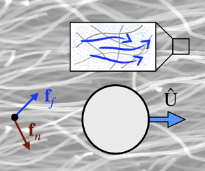
A consequence of the linearity of the governing equations is that any ambient displacement field can be expressed with a distribution of point forces in the fluid and network domains. This also includes the active stresses in cellular materials (used to maintain and rearrange their structures) that are typically described with distribution of forces, and force dipoles on the fluid and network phases in the continuum scale (Marchetti et al. Reference Marchetti, Joanny, Ramaswamy, Liverpool, Prost, Rao and Simha2013; Saintillan & Shelley Reference Saintillan and Shelley2015). Similarly, the presence of other immersed objects in a biphasic material can be modelled by distributions of point forces and higher-order singularities. In many instances the transport in cellular filamentous networks involve spherical (or sphere-like) objects, e.g. cell migration through the extracellular matrix (Camley & Rappel Reference Camley and Rappel2017), organelle transport throughout the cytoskeleton (Mogre, Brown & Koslover Reference Mogre, Brown and Koslover2020) and the dynamics of microinjected or endogenous probes in particle tracking microscopy (Weihs, Mason & Teitell Reference Weihs, Mason and Teitell2006). In these applications one must consider the movements of the spheres in response to active or passive forces/stresses in the medium. Motivated by this, and to show the utility of the reciprocal theorem, we consider a rigid spherical inclusion moving with a prescribed velocity  $\boldsymbol {U}$ in a PVE medium, subject to point forces $\boldsymbol {f}_{\{\,f,n\}}$ applied to fluid and network phases at some separation distance, $R$, from the centre of the sphere. Our goal is to derive a closed-form expression for the net force, $\boldsymbol {F}$, on the sphere in response to these point forces; see figure 2(a) for a schematic of this problem.

Figure 2. (a) The auxiliary problem in the implementation of the reciprocal theorem: a rigid sphere moving with a prescribed velocity  $\hat {\boldsymbol {U}}$ in a linear PVE medium with fluid shear viscosity $\eta$ and network shear modulus $G$ and Poisson ratio $\nu$. (b) The problem to be solved using reciprocal theorem: a rigid sphere moving with a prescribed velocity and subjected to external point forces in the fluid and the network phases, ${\boldsymbol {f}}_f$ and ${\boldsymbol {f}}_n$.
We assume the network is a linear elastic material with shear modulus  $G$ and Poisson ratio $\nu$, and the permeating fluid is Newtonian with shear viscosity $\eta$, so that $\tau (s)=s \eta /G=s\tau _\circ$, where $\tau _\circ =\eta /G$ is the shear relaxation time of the network in the fluid phase. However, the expressions that we are about to present are extendable to any other linear viscoelastic fluids and networks by modifying the expression for $\tau (s)$ in terms of constitutive parameters of the two phases. The flow fields and the net forces on the particle are first computed in Laplace space. We use Fourier–Euler summation (Abate & Whitt Reference Abate and Whitt1992) to numerically invert the results from $s$ space to time–space. The relative error of the numerical inversion is smaller than $10^{-9}$ in all the presented results.
To use the reciprocal theorem, we need a simple auxiliary problem that gives us  ${\hat {\boldsymbol {v}}}_{\{\,f,n\}}$ and ${\hat {\boldsymbol {\varSigma }}}_{\{\,f,n\}}$. We choose a sphere translating with velocity $\hat {\boldsymbol {U}}$ as our auxiliary problem. We derived these solutions in Moradi et al. (Reference Moradi, Shi and Nazockdast2022). Since the general solution is axisymmetric (see Appendix A), it can be expressed in the general form of
 $$\begin{gather} {\hat{\boldsymbol{v}}}_{f} = {\hat{\boldsymbol{U}}} \boldsymbol{\cdot} \left[ {A}_{f} \frac{\boldsymbol{r r}}{r^2} + {B}_{f} \left( \boldsymbol{I} - \frac{\boldsymbol{r r}}{r^2} \right) \right] , \quad {\hat{\boldsymbol{v}}}_{n} = {\hat{\boldsymbol{U}}} \boldsymbol{\cdot} \left[ {A}_{n} \frac{\boldsymbol{r r}}{r^2} + {B}_{n} \left( \boldsymbol{I} - \frac{\boldsymbol{r r}}{r^2} \right) \right], \end{gather}$$
 $$\begin{gather}{\hat{p}} = A_p {\hat{\boldsymbol{U}}} \boldsymbol{\cdot} \frac{\boldsymbol{r}}{r}. \end{gather}$$
Applying the BCs,  ${\hat {\boldsymbol {v}}}_{f} {|}_{r=a} = {\hat {\boldsymbol {U}}}$ and ${\hat {\boldsymbol {v}}}_{n} {|}_{r=a} = {\hat {\boldsymbol {U}}}$, specifies $A_{\{\,f,n\}}$ and $B_{\{\,f,n\}}$ as
 \begin{align} A_f &= \frac{1}{\varDelta} \left[ S_1 \left( \frac{a}{r} \right) + S_2 {\left( \frac{a}{r} \right)}^3 -3 \frac{a {\alpha}^2}{{\beta}^4 r^3} (1+ \beta r) \, {\rm e}^{-\beta (r-a)} \right], \end{align}
 \begin{align} B_f &= \frac{1}{\varDelta}
\left[ S_1 \left( \frac{a}{r} \right) - S_2 {\left(
\frac{a}{r} \right)}^3 +3 \frac{a {\alpha}^2}{{\beta}^4
r^3} (1+ \beta r + {\beta}^2 r^2 ) \, {\rm e}^{-\beta
(r-a)} \right],\end{align}
\begin{align} B_f &= \frac{1}{\varDelta}
\left[ S_1 \left( \frac{a}{r} \right) - S_2 {\left(
\frac{a}{r} \right)}^3 +3 \frac{a {\alpha}^2}{{\beta}^4
r^3} (1+ \beta r + {\beta}^2 r^2 ) \, {\rm e}^{-\beta
(r-a)} \right],\end{align} \begin{align}
A_n &=
\frac{1}{\varDelta} \left[ S_1 \left( \frac{a}{r} \right) -
S_3 {\left( \frac{a}{r} \right)}^3 + 3 \tau \frac{a
{\alpha}^2}{{\beta}^4 r^3} (1+ \beta r) \, {\rm e}^{-\beta
(r-a)} \right.\nonumber\\ &\quad\left. + 3 \frac{a
(1+\tau)}{{\beta}^2 r^3 } \, {\rm e}^{-\alpha (r-a)} \times
(2+2\alpha r + {\alpha}^2 r^2 ) \right],
\end{align}
\begin{align}
A_n &=
\frac{1}{\varDelta} \left[ S_1 \left( \frac{a}{r} \right) -
S_3 {\left( \frac{a}{r} \right)}^3 + 3 \tau \frac{a
{\alpha}^2}{{\beta}^4 r^3} (1+ \beta r) \, {\rm e}^{-\beta
(r-a)} \right.\nonumber\\ &\quad\left. + 3 \frac{a
(1+\tau)}{{\beta}^2 r^3 } \, {\rm e}^{-\alpha (r-a)} \times
(2+2\alpha r + {\alpha}^2 r^2 ) \right],
\end{align} \begin{align}
B_n &=
\frac{1}{\varDelta} \left[ S_1 \left( \frac{a}{r} \right) +
S_3 {\left( \frac{a}{r} \right)}^3 -3 \tau \frac{a
{\alpha}^2}{{\beta}^4 r^3} (1+ \beta r + {\beta}^2 r^2 ) \,
{\rm e}^{-\beta (r-a)} \right.\nonumber\\ &\quad\left. -6
\frac{a (1+\tau)}{{\beta}^2 r^3 } \, {\rm e}^{-\alpha
(r-a)} \times (1+\alpha r ) \right] ,
\end{align}
\begin{align}
B_n &=
\frac{1}{\varDelta} \left[ S_1 \left( \frac{a}{r} \right) +
S_3 {\left( \frac{a}{r} \right)}^3 -3 \tau \frac{a
{\alpha}^2}{{\beta}^4 r^3} (1+ \beta r + {\beta}^2 r^2 ) \,
{\rm e}^{-\beta (r-a)} \right.\nonumber\\ &\quad\left. -6
\frac{a (1+\tau)}{{\beta}^2 r^3 } \, {\rm e}^{-\alpha
(r-a)} \times (1+\alpha r ) \right] ,
\end{align} \begin{align} A_p &= \frac{G}{a \varDelta} \left[ \frac{1+\tau}{3} S_1 {\left( \frac{a}{r} \right)}^2 - 3 \tau {\left( \frac{a}{r} \right)}^2 (1+ \alpha r) \, {\rm e}^{-\alpha (r-a)} \right] , \end{align}
where
 \begin{align} &S_1 = 3 \tau \left( 1+ a \alpha + \frac{1}{2} \frac{{\alpha}^2}{{\beta}^2} (1+ a \beta + a^2 {\beta}^2) \right), \quad S_2 = \frac{{\alpha}^2}{a^2 {\beta}^4} (3+ 3a \beta + a^2 {\beta}^2 ) - \frac{1}{3} S_1, \end{align}
 \begin{align} &S_3 = \frac{2}{a^2 {\beta}^2} (3+3a \alpha + a^2 {\alpha}^2) + \frac{6+ a^2 {\beta}^2}{3 a^2 {\beta}^2} S_1, \quad \varDelta = \frac{{\alpha}^2}{{\beta}^2} + \frac{2}{3} S_1 . \end{align}
 Here,  ${\beta }^2 = {\beta }_{\circ }^2 (1+ \tau )$, with ${\beta }_{\circ } =\sqrt { {\xi }/{\eta }}$ being the inverse of permeability of the fluid and ${\alpha }^2 = s \tau _\circ \alpha _\circ ^2$, where $\alpha _\circ ^2={\beta }_{\circ }^2 (({ 1-2\nu })/{2(1-\nu )})$ with $\nu$ being the Poisson ratio. For an incompressible network, $\nu =0.5$ and $\alpha _\circ =0$. Substituting these values in the above equations cancels all the terms involving $\beta _\circ$ and reduces the expressions for $A_{\{\,f,n\}}$ and $B_{\{\,f,n\}}$ in (3.2), to their well-known form in Stokes flow:
 $$\begin{gather} A_{\{\,f,n\}}(\nu=0.5)=A_{Stokes}=\frac{3}{2} \left(\frac{a}{R}\right)-\frac{1}{2}\left(\frac{a}{R}\right)^3, \end{gather}$$
 $$\begin{gather}B_{\{\,f,n\}}(\nu=0.5)=B_{Stokes}=\frac{3}{4} \left(\frac{a}{R}\right)+\frac{1}{4}\left(\frac{a}{R}\right)^3. \end{gather}$$
We are interested in the dynamical features that arise due to network compressibility. Using the expressions in (3.1b), we can compute the traction applied by the fluid and the network phase on the surface of the sphere and integrate those on the sphere's surface to get the net force on the particle:
 \begin{equation} \left.\begin{array}{@{}c@{}} \displaystyle {\hat{\boldsymbol{F}}} = \int ( {\hat{\boldsymbol{\varSigma}}}_f + {\hat{\boldsymbol{\varSigma}}}_n ) \boldsymbol{\cdot} \boldsymbol{n}\, \mathrm{d}S \equiv{-} \mathcal{R} {\hat{\boldsymbol{U}}} , \\ \mathcal{R} = 6 {\rm \pi}\eta a \left[ \dfrac{ ( 1 + \tau ) (\alpha ^2 (a^2 \beta ^2+a \beta +1)+ 2 \beta ^2 (1+a\alpha) )}{ \tau ( \alpha ^2 (a^2 \beta ^2+a \beta +1)+2 \beta ^2 (1+a\alpha) )+\alpha ^2 } \right] . \end{array}\right\} \end{equation}
The term between the brackets is the correction to Stokes drag induced by network compressibility.
The second problem is the problem we seek to solve, which is shown in figure 2(b). We assume no-slip BCs for both the fluid and network on the surface of the sphere:  ${\boldsymbol {v}}_{\{\,f , n \}} (r=a) = \boldsymbol {U}$. No-slip BCs are generally valid for the fluid phase. The BCs for the network phase is more complex (Fu, Shenoy & Powers Reference Fu, Shenoy and Powers2010). When the particle size is much larger than the network's mesh size, $a\beta _\circ \gg 1$, the no-slip BC is a good approximation; this is the BC used in this section. In § 4.1 we discuss how the reciprocal theorem can be used to compute the leading-order effect of network slip on the dynamics of the sphere.
The point forces are expressed as  ${\boldsymbol {f}}_f = {\boldsymbol {f}}_{f}^{\circ } \delta (\boldsymbol {r}- \boldsymbol {R})$ and ${\boldsymbol {f}}_n = {\boldsymbol {f}}_{n}^{\circ } \delta (\boldsymbol {r}- \boldsymbol {R})$, where $\delta (\boldsymbol {r}- \boldsymbol {R})$ is the Dirac delta function. After substituting these expressions in (2.9) and a few simple lines of algebra we get
 \begin{equation} - \mathcal{R} \boldsymbol{U} + \boldsymbol{\mathcal{M}}_{f} \boldsymbol{\cdot} \boldsymbol{f}_{\!\!f}^{{\circ}} + \boldsymbol{\mathcal{M}}_{n} \boldsymbol{\cdot} \boldsymbol{f}_{\!\!n}^{{\circ}} = \boldsymbol{F},\end{equation}
where
 \begin{align} \boldsymbol{\mathcal{M}}_{f} = A_f (R) \frac{\boldsymbol{R R}}{R^2}+ B_f (R) \left( \boldsymbol{I} -\frac{\boldsymbol{RR}}{R^2} \right), \quad \boldsymbol{\mathcal{M}}_{n} = A_n (R) \frac{\boldsymbol{R R}}{R^2} + B_n (R) \left( \boldsymbol{I} - \frac{\boldsymbol{R R}}{R^2} \right). \end{align}
 Equations (3.6) and (3.7a,b) are the expressions we set out to derive. Here  $\boldsymbol {\mathcal {M}}_{f}$ and $\boldsymbol {\mathcal {M}}_{n}$ are the response functions that relate the forces on fluid and network phases to the net force and velocity of the spherical particle. For a force-free particle (mobility problem), we can set $\boldsymbol {F}=0$, which yields
 \begin{equation}\boldsymbol{U}=\mathcal{R}^{{-}1}(\boldsymbol{\mathcal{M}}_{f} \boldsymbol{\cdot} \boldsymbol{f}_{\!\!f}^{{\circ}} + \boldsymbol{\mathcal{M}}_{n} \boldsymbol{\cdot} \boldsymbol{f}_{\!\!n}^{{\circ}} ),\end{equation}
In this set-up,  $\boldsymbol {\mathcal {M}}_{f}$ and $\boldsymbol {\mathcal {M}}_{n}$ can be thought of as mobility tensors that relate the forces on each phase to the particle's velocity. For brevity, we only present the results of the fixed particle (resistance problem), $\boldsymbol {U}=\boldsymbol {0}$, in the next section. The solution can easily be extended to force-free particles (mobility problem), using (3.8).
3.1. Net force on a fixed sphere
We consider the special case of a fixed particle,  $\boldsymbol {U} =\boldsymbol {0}$, which simplifies (3.6) to
 \begin{equation} \boldsymbol{U}=\boldsymbol{0}:\quad \boldsymbol{F}=\boldsymbol{\mathcal{M}}_{f} \boldsymbol{\cdot} \boldsymbol{f}_{\!\!f}^{{\circ}} + \boldsymbol{\mathcal{M}}_{n} \boldsymbol{\cdot} \boldsymbol{f}_{\!\!n}^{{\circ}}. \end{equation}
It is useful to decompose the point forces and the force on the particle in parallel and perpendicular directions of the separation vector. Using  $\boldsymbol {f}_{\{\,f,n\}}^{\circ } = {f}_{\{\,f,n\}}^{\parallel } \hat {\boldsymbol {R}} + {f}_{\{\,f,n\}}^{\perp } \hat {\boldsymbol {R}}^{\perp }$ and $\boldsymbol {F}=F^\parallel \hat {\boldsymbol {R}}+F^\perp \hat {\boldsymbol {R}}^{\perp }$, we get
 \begin{equation} {F}^{{\parallel}} = A_f (R) {f}_f^{{\parallel}} + A_n (R) {f}_n^{{\parallel}} ,\quad {F}^{{\perp}} = B_f (R) {f}_f^{{\perp}} + B_n (R) {f}_n^{{\perp}} . \end{equation}
 We begin by analysing the limiting behaviours of  $A_{\{\,f,n\}}$ and $B_{\{\,f,n\}}$ at early ( $t\to 0$) and long ( $t\to \infty$) times. These limits can be computed analytically using the following relationships: $f(t\to 0^+)= \lim _{s\to \infty } s f(s)$ and $f(t\to \infty )= \lim _{s\to 0} s f(s)$ and the results are
 \begin{align} {A}_{ \{\,f , n\} } (t\to
0)&= \frac{3}{2} \left( \frac{a}{R} \right) -\frac{1}{2}
{\left( \frac{a}{R} \right)}^3 , \quad {B}_{ \{\,f , n\} }
(t\to 0)= \frac{3}{4} \left( \frac{a}{R} \right) +
\frac{1}{4} {\left( \frac{a}{R} \right)}^3 ,
\end{align}
\begin{align} {A}_{ \{\,f , n\} } (t\to
0)&= \frac{3}{2} \left( \frac{a}{R} \right) -\frac{1}{2}
{\left( \frac{a}{R} \right)}^3 , \quad {B}_{ \{\,f , n\} }
(t\to 0)= \frac{3}{4} \left( \frac{a}{R} \right) +
\frac{1}{4} {\left( \frac{a}{R} \right)}^3 ,
\end{align} \begin{align}
A_f (t\to \infty) &=
\frac{6(1-\nu)}{5-6\nu} \left( \frac{a}{R} \right) -
\frac{1}{5-6\nu} {\left( \frac{a}{R} \right)}^3 \nonumber\\
& \quad + \frac{3a(1-2\nu)}{{\beta}_{{\circ}}^2 R^3
(5-6\nu)} [ 1+a {\beta}_{{\circ}} -(1+ {\beta}_{{\circ}} R
)\times {\mathrm{e}}^{-{\beta}_{{\circ}} (R-a)} ] ,
\end{align}
\begin{align}
A_f (t\to \infty) &=
\frac{6(1-\nu)}{5-6\nu} \left( \frac{a}{R} \right) -
\frac{1}{5-6\nu} {\left( \frac{a}{R} \right)}^3 \nonumber\\
& \quad + \frac{3a(1-2\nu)}{{\beta}_{{\circ}}^2 R^3
(5-6\nu)} [ 1+a {\beta}_{{\circ}} -(1+ {\beta}_{{\circ}} R
)\times {\mathrm{e}}^{-{\beta}_{{\circ}} (R-a)} ] ,
\end{align} \begin{align}
B_f(t\to \infty) &= \frac{3(1-\nu)}{5-6\nu} \left( \frac{a}{R}
\right) + \frac{1}{2(5-6\nu)} {\left( \frac{a}{R}
\right)}^3 \nonumber\\ & \quad - \frac{3a(1-2\nu)}{2
{\beta}_{{\circ}}^2 R^3 (5-6\nu)} [ 1+a {\beta}_{{\circ}}
-(1+ {\beta}_{{\circ}} R+ {\beta}_{{\circ}}^2 R^2 ) \times
{\mathrm{e}}^{-{\beta}_{{\circ}} (R-a)} ] ,
\end{align}
\begin{align}
B_f(t\to \infty) &= \frac{3(1-\nu)}{5-6\nu} \left( \frac{a}{R}
\right) + \frac{1}{2(5-6\nu)} {\left( \frac{a}{R}
\right)}^3 \nonumber\\ & \quad - \frac{3a(1-2\nu)}{2
{\beta}_{{\circ}}^2 R^3 (5-6\nu)} [ 1+a {\beta}_{{\circ}}
-(1+ {\beta}_{{\circ}} R+ {\beta}_{{\circ}}^2 R^2 ) \times
{\mathrm{e}}^{-{\beta}_{{\circ}} (R-a)} ] ,
\end{align} \begin{align} A_n (t\to \infty) &= \frac{6(1-\nu)}{5-6\nu} \left( \frac{a}{R} \right) - \frac{1}{5-6\nu} {\left( \frac{a}{R} \right)}^3 , \end{align}
 \begin{align} B_n (t\to \infty) &= \frac{3(3-4\nu)}{2(5-6\nu)} \left( \frac{a}{R} \right) + \frac{1}{2(5-6\nu)} {\left( \frac{a}{R} \right)}^3. \end{align}
 As shown in (3.11a), at short times the response functions for both fluid and network asymptote to their well-known respective forms in Stokes flow (Kim & Karrila Reference Kim and Karrila2013). This can be explained by noting that at early times the network co-moves with the fluid phase,  $\boldsymbol {v}_n(\boldsymbol {r},t\to 0)=\boldsymbol {v}_f(\boldsymbol {r},t\to 0)$ and $\boldsymbol {\nabla } \boldsymbol {\cdot } \boldsymbol {v}_{\{\,f,n\}}(\boldsymbol {r},t\to 0)=0$. Furthermore, at long times the response functions of the network phase ( $A_n$ and $B_n$), approach their well-known form in linear elasticity (Phan-Thien & Kim Reference Phan-Thien and Kim1994); see (3.11d) and (3.11e). The long time forms of the fluid response functions ( $A_f$ and $B_f$) include extra $\beta _\circ$ dependent terms, which, as expected, become identically zero for an incompressible network.
Variations of the net force with time and the distance from the point forces in the parallel direction are determined by the behaviour of  $A_{\{\,f,n\}}$. Since we have the analytical form of these functions in short and long times in (3.11), we study the time-dependent behaviour of the following quantities:
 \begin{align} \hat{A}_{\{\,f,n\}}= \frac{A_{\{\,f,n\}}(t,R)-A_{\{\,f,n\}}(t\to \infty,R)}{A_{\{\,f,n\}}(0,R)-A_{\{\,f,n\}}(t\to \infty,R)},\quad \hat{B}_{\{\,f,n\}}=\frac{B_{\{\,f,n\}}(t,R)-B_{\{\,f,n\}}(t\to \infty,R)}{B_{\{\,f,n\}}(0,R)-B_{\{\,f,n\}}(t\to \infty,R)}.\end{align}
Here  $\hat {A}$ and $\hat {B}$, by construction relax over time from $\hat {A}=\hat {B}=1$ at $t=0$ to $\hat {A}=\hat {B}\to 0$ as $t\to \infty$. Next, we explore how the relaxation dynamics changes with the separation distance, $R$, and material properties of the fluid and network, $\eta, G, \beta _\circ$ and $\nu$.
The expressions for  $A_{\{\,f,n\}}$ and $B_{\{\,f,n\}}$ in (3.2) contain two types of $s$ and $R$ dependencies. One obvious relaxation mechanism is shear relaxation, $\tau _\circ =\eta /G$, which is independent of $\beta _\circ$ and $\nu$ and the separation distance, $R$. This is the relaxation time measured in the standard particle tracking microrheology. The terms involving $S_1$, $S_2$ and $S_3$ can be written as a product of only $s$-dependent and only $r$-dependent functions, $\tilde {\mathcal {Q}}(s) \mathcal {P}(r)$, resulting in a $\mathcal {Q}(t) \mathcal {P}(r)$ form after Laplace inversion. As a result, the relaxation behaviour becomes independent of $R$. In comparison, the terms that include $\exp (-\beta (s) r)$ and $\exp (-\alpha (s) r)$ cannot be written as a product of $s$- and $r$-dependent functions, and so the relaxation time of the force on the sphere becomes a function of the distance from the point forces.
As shown in our earlier work (Moradi et al. Reference Moradi, Shi and Nazockdast2022) and others (Detournay & Cheng Reference Detournay and Cheng1993; Doi Reference Doi2009), the divergence of the displacement field in a linear elastic network,  $\boldsymbol {\nabla } \boldsymbol {\cdot } \boldsymbol {v}_n$, is described by a diffusion equation, where the diffusion coefficient is $D=\tau _\circ \alpha _\circ ^{-2}$. Based on this, we can introduce two extra time scales: $\tau _D^a=(\alpha _\circ a)^2\tau _\circ$, which is the time scale for the network compressibility to diffuse over a particle radius, $a$; and $\tau _D^{R}=(\alpha _\circ R)^2\tau _\circ$ is the time for diffusing a distance $R$ from the point forces.
If the  $S_1$, $S_2$ and $S_3$ terms dominate the response, we expect the force relaxation time to be independent of $R$ and determined by $\tau _D^ a$; alternatively, if $\exp (-\alpha (s) r)$ and $\exp (-\beta (s) r)$ terms determine the behaviour of $A_{\{\,f,n\}}$ and $B_{\{\,f,n\}}$, we expect the force relaxation to be distance dependent and in part determined by $\tau _D^{R}$.
We begin with presenting the results for the relaxation dynamics of fluid phase functions  $\hat {A}_f$ and $\hat {B}_f$ versus time in figure 3 for different values of Poisson ratio, $\nu$ (figure 3a), permeability, $\beta _\circ$ (figure 3b) and distance from the point force $R$ (figure 3c). The solid lines that go through the markers are the computed values of $\widehat {(S_1/\varDelta )}$, which is simply the values of $S_1/\varDelta$ made dimensionless in the exact manner as $A_f$ and $B_f$ in (3.2). The relaxation time is made dimensionless with $\tau _D^a$ in all figures. When $R$ is fixed and $\nu$ and $\beta _\circ$ are varied (figure 3a,b), $\tau _D^a$ and $\tau _D^R$ are linearly related by a constant factor, $\tau _D^R/\tau _D^a = (R/a)^2$, and using $\tau _D^R$ (instead of $\tau _D^a$) would only shift the plots in the $x$ axis and would not change the overall superposition of the curves. In comparison, when $R$ is varied, the two time scales become distinct. Thus, to test if the relaxation is distance dependent or not, we present the results of figure 3(c) as a function of $t/\tau _D^R$ in the insets of those figures.

Figure 3. Time variations of the fluid hydrodynamic functions,  $\hat {A}_f$ (top row) and $\hat {B}_f$ (bottom row). (a) Different values of Poisson ratio, $\nu$, while setting $\beta _\circ =5$ and $R=2$. (b) Different values of permeability, $\beta _\circ$, while setting $\nu =0.3$ and $R=2$. (c) Different separation distances, $R$, while setting $\nu =0.3$ and $\beta _\circ =5$. The time axis is made dimensionless with $\tau _D^a=a^2\alpha _\circ ^2\tau _\circ$ in all the main plots. The values of $R$ and $\beta _\circ$ are made dimensionless with the sphere radius, which is equivalent to taking $a:=1$. The inset figures in figure 3(c) show the same results as the main figure, but the time axes are made dimensionless with $\tau _D^R=R^2\alpha _\circ ^2\tau _\circ$.
As can be seen, in all cases  $\widehat {(S_1/\varDelta )}$ (solid lines) closely match the predictions that include all the terms (symbols). This suggests that the relaxation is distance independent and that $\tau _D^a$ (and not $\tau _D^R$) is a more appropriate choice for relaxation time of $\hat {A}_f$ and $\hat {B}_f$. This can be clearly seen by comparing the nearly perfect superposition of the plots in the main figure against the inset plots in figure 3(c). Furthermore, the relaxation curves for different values of $\nu$ superimpose, when time is made dimensionless with $\tau _D^a$. The superposition is not as clean at shorter times when permeability is varied (see figure 3b), since shear relaxation time ( $\tau _\circ$) becomes increasingly more important at shorter time scales, where the fluid and network phase co-move. However, at longer times ( $t/\tau _D^a\ge 10$) the plots superimpose, showing that the long time behaviour of these hydrodynamic functions is determined by $\tau _D^a$. Collectively, these results show that the relaxation dynamics of $\hat {A}_{f}$ and $\hat {B}_f$ is not distance dependent, and is dominated by the terms involving $(S_1/\varDelta )(a/r)$ and the relaxation time, $\tau _D^a$.
Figure 4 shows the relaxation dynamics of the network functions,  $\hat {A}_n$ and $\hat {B}_n$. In this case, the solid lines are just showing the detailed predictions and are not showing $\widehat {(S_1/\varDelta )}$, since $\widehat {(S_1/\varDelta )}$ values did not match the detailed predictions. The time axis is made dimensionless by $\tau _D^{R}$ in all the main plots. Again, when the separation distance is varied, we replot the results of figure 4(c) in the inset figure, but with the dimensionless time being defined as $t/\tau _D^a$. As can be seen in figure 4(c), using $t/\tau _D^R$ gives a better collapse of the relaxation plots at long times and at different $R$ in the main plot, compared with the inset figures, with $t/\tau _D^a$ as the $x$ axis. However, the collapse is not as clean as the results for $\hat {A}_f$ and $\hat {B}_f$. For both cases of varying permeability and distance (figures 4b and 4c), the plots fail to collapse at shorter times, especially for $\hat {B}_n$, where the shape of the plots qualitatively changes with varying $\beta _\circ$ and $R$.
$R$.

Figure 4. Time variations of the network hydrodynamic functions,  $\hat {A}_n$ (top row) and $\hat {B}_n$ (bottom row). (a) Different values of Poisson ratio, $\nu$, while setting $\beta _\circ =5$ and $R=2$. (b) Different values of permeability, $\beta _\circ$, while setting $\nu =0.3$ and $R=2$. (c) Different separation distances, $R$, while setting $\nu =0.3$ and $\beta _\circ =5$. The time axis is made dimensionless with $\tau _D^R=R^2\alpha _\circ ^2\tau _\circ$ in all the main plots. The inset figures in figure 4(c) show the same results as the main figure, but the time axes are made dimensionless with $\tau _D^a=a^2\alpha _\circ ^2\tau _\circ$.
All together these results suggest that the relaxation behaviour of the network functions  $\hat {A}_n$ and $\hat {B}_n$ at long times is distance dependent and best described by $\tau _D^{R}$. However, at shorter times the fluid shear stress plays a more central role and the relaxation dynamics is a function of all three time scales ( $\tau _\circ$, $\tau _D^a$ and $\tau _D^R$). Including the shear stresses in the conservation equations allows us to study the complex variations in the relaxation behaviour from short to long time scales.
4. Other applications
In this section we give a brief overview of some of the other applications of the reciprocal theorem for PVE materials. Our focus here is to derive the final expressions (in form of surface and volume integrals) for each application, without evaluating these expressions and discussing the results for different choices of parameters.
4.1. Slip BC for the network phase
In deriving the expressions for the sphere's response to point forces, we assumed a no-slip BC for the network phase at the sphere's surface. This assumption generally holds when the size of the sphere is considerably larger than the network and there is no active interactions between the network and the sphere. As an example, the mesh size for actin networks in the cell is roughly in the range 20–200 nm (Charras et al. Reference Charras, Yarrow, Horton, Mahadevan and Mitchison2005; Keren et al. Reference Keren, Yam, Kinkhabwala, Mogilner and Theriot2009), and so the no-slip BC is appropriate for micron-sized endogenous bodies and injected probes used in microrheological measurements. But in many cases, such as transport of proteins and nanoscopic particles, the size of the inclusion can become comparable or smaller than the mesh size. In such conditions, we must account for slip velocity between the inclusion and the network phase (a no-slip BC generally holds for the fluid phase down to atomistic lengths).
One method of modelling the slip velocity is to use the equivalent of the Navier equation, where the tangential slip velocity is proportional to the traction in that direction, i.e.
 \begin{equation} \boldsymbol{v}_n =\boldsymbol{U}+\frac{b}{\mu}(\boldsymbol{I}-\boldsymbol{n} \boldsymbol{n}) \boldsymbol{\cdot} (\boldsymbol{\varSigma}_n \boldsymbol{\cdot} \boldsymbol{n}), \end{equation}
where  $b$ is the slip length and $\mu$ is the term with dimensions of viscosity. Recall that the above equation is written in Laplace space. The time dependence of $\mu$ depends on the mechanical coupling of the network with the sphere's surface in microscopic scale. For example, if the network is not tethered to the boundary, we may assume that the slip dynamics is viscous, and take $\mu (t)=\mu _\circ \to \mu (s)=\mu _\circ /s$; in the opposite case of the network tethered to the boundary, the slip dynamics may be predominantly elastic, leading to slip displacements rather than slip velocities: $\mu (t)=\mu _\circ \delta (t) \to \mu (s)=\mu _\circ$. In any case, we recover a no-slip BC when $b=0$.
Our goal is to find the leading-order correction to the force on a sphere moving with velocity  $\boldsymbol {U}$, subject to this BC. We would like to avoid solving this boundary value problem by using the reciprocal theorem. We use the sphere moving with velocity $\hat {\boldsymbol {U}}$, with a no-slip BC for both phases as our auxiliary problem, and use the slip BC for the network as our target solution. Upon substitution we find that
 \begin{equation} \boldsymbol{F} \boldsymbol{\cdot} {\hat{\boldsymbol{U}}}= {\hat{\boldsymbol{F}}} \boldsymbol{\cdot} \boldsymbol{U}+\left(\frac{b}{\mu}\right) \int_{S_p} ( {\hat{\boldsymbol{\varSigma}}}_n \boldsymbol{\cdot} \boldsymbol{n})\boldsymbol{\cdot} [(\boldsymbol{I}-\boldsymbol{n}\boldsymbol{n})\boldsymbol{\cdot} (\boldsymbol{\varSigma}_n\boldsymbol{\cdot} \boldsymbol{n})] \,\mathrm{d}S.\end{equation}
Next, we assume a small slip length ( ${b}/{a}\ll 1$), and so we can write down the following perturbation expansions:
 \begin{equation} \boldsymbol{v}_n = {\hat{\boldsymbol{v}}}_n +\left(\frac{b}{a}\right)\boldsymbol{v}_{n}^{(1)} +O\left[\left(\frac{b}{a}\right)^2\right],\quad \boldsymbol{\varSigma}_n ={\hat{\boldsymbol{\varSigma}}}_n + \left(\frac{b}{a}\right) \boldsymbol{\varSigma}_n^{(1)} +O\left[\left(\frac{b}{a}\right)^2\right]. \end{equation}
Substituting these expansions into (4.2), replaces  $\boldsymbol {\varSigma }_n$ with ${\hat {\boldsymbol {\varSigma }}}_n$, and so we get
 \begin{equation} \boldsymbol{F} \boldsymbol{\cdot} {\hat{\boldsymbol{U}}} = {\hat{\boldsymbol{F}}} \boldsymbol{\cdot} \boldsymbol{U}+\left(\frac{b}{\mu}\right) \int_{S_p} [ ({\hat{\boldsymbol{\tau}}}_n\boldsymbol{\cdot} {\hat{\boldsymbol{\tau}}}_n )-({\hat{\boldsymbol{\tau}}}_n \boldsymbol{\cdot} \boldsymbol{n})^2] \,\mathrm{d}S +O\left[\left(\frac{b}{a}\right)^2\right],\end{equation}
where  ${\hat {\boldsymbol {\tau }}}_n={\hat {\boldsymbol {\varSigma }}}_n \boldsymbol {\cdot } \boldsymbol {n}$ is the network traction of the auxiliary problem. We see that the reciprocal theorem can be used to compute the first-order correction to the drag due to slip in the network phase. Almost the exact same derivation can be used to model the slip BC in Stokes flow, as outlined in Masoud & Stone (Reference Masoud and Stone2019).
When the inclusion is considerably smaller than the mesh ( $b/a\gg 1$), it can move through the network pores and channels without experiencing any force from the network. In this limit, no network traction, $\boldsymbol {\varSigma }_n \boldsymbol {\cdot } \boldsymbol {n}=0$ at $|\boldsymbol {r}|=a$ would be a more appropriate BC. In this scenario and under a constant external force, the sphere will move with a steady-state velocity (viscous response) with the fluid velocity and the sphere's drag determined by the Brinkman equation. In comparison, when a no-slip BC is assumed for the network, as we showed earlier, the long time behaviour of the sphere under a constant force will be elastic.
Let us now consider the auxiliary problem of a sphere moving with velocity  $\hat {\boldsymbol {U}}$, but this time with a no-slip BC only applied to the fluid domain and zero traction BCs applied for the network phase. It is straightforward to find the displacement fields for this problem, using the general solutions of PVE equations (Moradi et al. Reference Moradi, Shi and Nazockdast2022). Fu, Shenoy & Powers (Reference Fu, Shenoy and Powers2008) also provide a closed-form solution of this problem. Assuming that we have the solution for this auxiliary problem, we would like to find the net force on the sphere moving with velocity $\boldsymbol {U}$ and subjected to point forces in the fluid and network phases, using no traction from the network as a BC. After substituting the auxiliary solution to the reciprocal theorem, and applying the BC, we recover (3.6) and (3.7a,b), with the distinction that $A_{\{\,f,n\}}$ and $B_{\{\,f,n\}}$ now correspond to the auxiliary problem with zero network traction as the BC.
Finally, we ask if the combination of perturbation methods and the reciprocal theorem can be used to find the sphere's response functions to point forces, subject to the slip BC given by (4.1). Again, we use the sphere moving with velocity  $\hat {\boldsymbol {U}}$ with no-slip BCs for both phases as the auxiliary problem, and seek to find the net force on the sphere in response to point forces $\boldsymbol {f}_{\{\,f,n\}} =\boldsymbol {f}_{\{\,f,n\}}^{\circ } \delta (\boldsymbol {r} - \boldsymbol {R})$, with the network BC given by (4.1). After substitution and using $b/a\ll 1$ we get
 \begin{align} \boldsymbol{F} \boldsymbol{\cdot} {\hat{\boldsymbol{U}}} &= {\hat{\boldsymbol{F}}} \boldsymbol{\cdot} \boldsymbol{U}+{\hat{\boldsymbol{v}}}_f (\boldsymbol{R}) \boldsymbol{\cdot} \boldsymbol{f}_{\!\!f}^{{\circ}}+{\hat{\boldsymbol{v}}}_n(\boldsymbol{R})\boldsymbol{\cdot} \boldsymbol{f}_{\!\!n}^{{\circ}} \nonumber\\ &\quad +\left(\frac{b}{\mu}\right) \int_{S_p} ( {\hat{\boldsymbol{\varSigma}}}_n \boldsymbol{\cdot} \boldsymbol{n})\boldsymbol{\cdot} [(\boldsymbol{I}-\boldsymbol{n}\boldsymbol{n})\boldsymbol{\cdot} (\boldsymbol{\varSigma}_n^{(0)} \boldsymbol{\cdot} \boldsymbol{n})] \,\mathrm{d}S +O\left[\left(\frac{b}{a}\right)^2\right]. \end{align}
The first line of (4.5) is exactly the expression we get using the no-slip BC in both phases. The second line shows the correction to the net force on the sphere due to network slip. Here,  $\boldsymbol {\varSigma }_n^{(0)}$ is the network stress in the target problem with a no-slip BC in both phases. Thus, we see that using the reciprocal theorem comes with the caveat of having to solve the problem of a sphere subjected to point forces, with a no-slip BC in both phases. Of course, the solution can be obtained, using the general solutions and the fundamental solutions to point forces in the fluid and network phase, but the calculations are lengthy and will not be pursued here.
4.2. Nonlinearities in the fluid and network forces and stresses
Another utility of the reciprocal theorem in fluid mechanics is in calculating the leading-order effects of nonlinear viscoelastic stresses (Leal Reference Leal1980; Hu & Joseph Reference Hu and Joseph1999; Koch & Subramanian Reference Koch and Subramanian2006; Khair & Squires Reference Khair and Squires2010; Elfring Reference Elfring2015) and finite inertia (Ho & Leal Reference Ho and Leal1974) in the net force and velocity of a particle, without the need to directly solve the nonlinear problem. See Masoud & Stone (Reference Masoud and Stone2019) for a comprehensive review of the topic.
The same ideas can be directly applied to study the nonlinear effects in biphasic systems. To demonstrate this point, we reconsider the problem of a sphere moving a prescribed velocity  $\boldsymbol {U}$ in an isotropic elastic network and a Newtonian fluid (with a no-slip BC in both phases), and derive an expression that allows computing the leading-order correction to the sphere's drag due to nonlinear terms that appear in the equations in finite deformations. One possible source of nonlinearity in the problem is the contribution of hyperelastic stresses in finite deformations of the elastic network. The simplest hyperelastic model is the Saint Venant–Kirchhoff model (Nezamabadi, Zahrouni & Yvonnet Reference Nezamabadi, Zahrouni and Yvonnet2011), where a linear stress–strain relationship is still assumed and only geometric nonlinearities are accounted for. We choose this model for its simplicity, but the methodology can be directly used for other choices of hyperelastic models that reduce to linear elasticity in small deformations. In the Saint Venant–Kirchhoff model the elastic stress in Eulerian coordinates is given by
 \begin{equation} \boldsymbol{\sigma}_n = 2G \boldsymbol{e} +\lambda \,\text{trace}(\boldsymbol{e}),\quad \boldsymbol{e}=\tfrac{1}{2}[\boldsymbol{\nabla} \boldsymbol{u}_n+(\boldsymbol{\nabla} \boldsymbol{u}_n)^T] - \boldsymbol{\nabla} \boldsymbol{u}_n\boldsymbol{\cdot} (\boldsymbol{\nabla} \boldsymbol{u}_n)^T, \end{equation}
where  $\boldsymbol {e}$ is the Eulerian finite strain tensor, which also includes the nonlinear term that is the product of the displacement gradient and its transpose. Another source on nonlinearity is in the term that models the relative frictional forces between the fluid and network, $\xi (\partial \boldsymbol {u}_n/\partial t -\boldsymbol {v}_f)$. Specifically, the partial time derivative of the displacement field ( $\partial \boldsymbol {u}_n/\partial t$) must be replaced with the velocity of material elements (Fu et al. Reference Fu, Shenoy and Powers2010), which is defined as $\textrm {d}\boldsymbol {u}_n/\textrm {d}t =\partial \boldsymbol {u}_n/\partial t + (\textrm {d}/\textrm {d}t)(\boldsymbol {u}_n(t) \boldsymbol {\cdot } \boldsymbol {\nabla } \boldsymbol {u}_n(t))$.
We use perturbation expansion of the displacement and stress fields and the net force, i.e.
 \begin{equation} \boldsymbol{v}_{\{\,f,n\}}=\boldsymbol{v}^{(0)}_{\{\,f,n\}} + \boldsymbol{v}^{(1)}_{\{\,f,n\}}, \quad \boldsymbol{\varSigma}_{\{\,f,n\}}=\boldsymbol{\varSigma}^{(0)}_{\{\,f,n\}} + \boldsymbol{\varSigma}^{(1)}_{\{\,f,n\}},\quad \boldsymbol{F}=\boldsymbol{F}^{(0)}+\boldsymbol{F}^{(1)}, \end{equation}
and assume a no-slip BC, which reduces to the following BCs for  $\boldsymbol {v}^{(0)}$ and $\boldsymbol {v}^{(1)}$:
 \begin{equation} \boldsymbol{v}_{\{\,f,n\}} ^{(0)} (|\boldsymbol{r}|=a)=\boldsymbol{U}, \quad \boldsymbol{v}_{\{\,f,n\}}^{(1)} (|\boldsymbol{r}|=a) =\boldsymbol{0}. \end{equation}
The solution to the linear problem is known:  $\boldsymbol {F}^{(0)}=-\mathcal {R}\boldsymbol {U}$. Importantly, $\boldsymbol {v}^{(1)}_{\{\,f,n\}}$ are also described by linear biphasic equations with the difference that the equations also include body forces that are only dependent on the solution of the linear problem:
 $$\begin{gather} \boldsymbol{\nabla} \boldsymbol{\cdot} \boldsymbol{\varSigma}_f^{(1)}+ \xi (\boldsymbol{v}^{(1)}_n - \boldsymbol{v}^{(1)}_f ) ={-}\boldsymbol{f}_{\!\!f},\quad \boldsymbol{f}_{\!\!f}=s\mathcal{L}[\boldsymbol{u}_n^{(0)} (t)\boldsymbol{\cdot} \boldsymbol{\nabla} \boldsymbol{u}^{(0)}_n(t)], \end{gather}$$
 $$\begin{gather}\boldsymbol{\nabla} \boldsymbol{\cdot} \boldsymbol{\varSigma}_n^{(1)} - \xi (\boldsymbol{v}^{(1)}_n - \boldsymbol{v}^{(1)}_f ) ={-}\boldsymbol{f}_{\!\!n},\quad \boldsymbol{f}_{\!\!n}=\mathcal{L}[\boldsymbol{\nabla} \boldsymbol{\cdot} \boldsymbol{\sigma}^{(0)}_{n,{n.l}}(t)]- s\mathcal{L}[\boldsymbol{u}_n^{(0)}(t)\boldsymbol{\cdot} \boldsymbol{\nabla} \boldsymbol{u}_n^{(0)}(t)]. \end{gather}$$
Here  $\boldsymbol {\sigma }^{(0)}_{n, {n.l}}=-2G[\boldsymbol {\nabla } \boldsymbol {u}_n^{(0)} \boldsymbol {\cdot } (\boldsymbol {\nabla } \boldsymbol {u}_n^{(0)})^T]-\lambda \, \textrm {trace}[\boldsymbol {\nabla } \boldsymbol {u}_n^{(0)} \boldsymbol {\cdot } (\boldsymbol {\nabla } \boldsymbol {u}_n^{(0)})^T]$ is the nonlinear piece of the elastic stress evaluated from the linear solution.
Next, we use the reciprocal theorem to find the drag contribution for the nonlinear terms,  $\boldsymbol {F}^{(1)}$, without directly solving (4.9). We use the solution to the linear problem with no body force as our auxiliary problem. Upon substitution we get
 \begin{equation} {\boldsymbol{F}} \boldsymbol{\cdot} {\hat{\boldsymbol{U}}} =\int_V ({\hat{\boldsymbol{v}}}_f\boldsymbol{\cdot} \boldsymbol{f}_{\!\!f}+{\hat{\boldsymbol{v}}}_n \boldsymbol{\cdot} \boldsymbol{f}_{\!\!n} )\, \mathrm{d}V, \end{equation}
where  ${\hat {\boldsymbol {U}}} := \boldsymbol {U}$, ${\boldsymbol {F}} :=\boldsymbol {F}^{(1)}$ and $\hat {\boldsymbol {v}}_{\{\,f,n\}} := \boldsymbol {v}_{\{\,f,n\}}^{(0)}$. Thus, $\boldsymbol {F}^{(1)}$ can be computed by evaluating the integral involving only known terms. Analytical evaluation of this integral is tedious, but the numerical integration is straightforward.
The same methodology can be used to account for weak nonlinear stresses in the fluid phase, due to viscoelasticity (small Deborah numbers), or shear rate-dependent viscosity (Leal Reference Leal1980; Elfring & Lauga Reference Elfring and Lauga2015; Boyko & Stone Reference Boyko and Stone2021).
4.3. Self-propulsion in biphasic systems
Another major application of the reciprocal theorem is in modelling the self-propulsion of active biological or synthetic entities at low Reynolds flows (Becker et al. Reference Becker, Koehler and Stone2003; Lauga & Powers Reference Lauga and Powers2009; Masoud & Stone Reference Masoud and Stone2014; Elfring Reference Elfring2015; Li et al. Reference Li, Lauga and Ardekani2021). As with the previous examples, the framework in Stokes flow can be directly extended to biphasic systems. We focus on the general case, where the active interactions between the motile object with the biphasic medium leads to slip velocities on the surface of the object with respect to the network and the fluid phases. The exact form of this slip velocity depends very much on the specifics of the involved active processes in smaller scales. For the purpose of this discussion, we assume the slip velocities in both phases,  $\boldsymbol {v}_{\{\,f,n\}}^s$, are known. Our goal is to find the net propulsion speed of the force-free particle, $\boldsymbol {U}$, due to these surface activities. Hence, the velocity on the particle's surface is $\boldsymbol {v}_{\{\,f,n\}}=\boldsymbol {U}+\boldsymbol {v}^s_{\{\,f,n\}}$.
We use the solution to a particle moving with  ${\hat {\boldsymbol {U}}}$ under a no-slip BC as the auxiliary solution, and seek to find $\boldsymbol {U}$. After substitution we get
 \begin{equation} {\hat{\boldsymbol{F}}} \boldsymbol{\cdot} \boldsymbol{U}={-}\int_{S_p} (\boldsymbol{v}^s_{f}\boldsymbol{\cdot} {\hat{\boldsymbol{\varSigma}}}_f + \boldsymbol{v}^s_{n}\boldsymbol{\cdot} {\hat{\boldsymbol{\varSigma}}}_n )\boldsymbol{\cdot} \boldsymbol{n} \, \mathrm{d}S, \end{equation}
where we used the force-free condition on the motile particle ( $\int _{S_p} (\boldsymbol {\varSigma }_f +\boldsymbol {\varSigma }_n )\boldsymbol {\cdot } \boldsymbol {n} \, \mathrm {d} S=\boldsymbol {0}$) to derive the final expression. This expression holds for any particle shape, but is only useful if the solution to the auxiliary problem is either known or can be obtained more easily using analytical and numerical methods. This formulation is also extendable to a collection of particles (Elfring Reference Elfring2015; Papavassiliou & Alexander Reference Papavassiliou and Alexander2015).
5. Summary
A reciprocal theorem was developed for a two-phase PVE material composed of a linear compressible viscoelastic network that is permeated by a linear viscoelastic fluid. The theorem is expressed in (2.9) and, like its counterparts in Stokes flow and linear elasticity, is applicable to anisotropic linear materials.
As an application of the reciprocal theorem, we analytically calculated the net force on a rigid stationary sphere due to point forces in the fluid and network phases outside of the sphere. We chose the solution to a sphere moving with a prescribed velocity in the PVE medium (Moradi et al. Reference Moradi, Shi and Nazockdast2022) as the auxiliary solution. We showed that the time evolution of the net force due to a point force in a Newtonian fluid permeating a linear compressible elastic network is independent of the distance between the point force and the sphere, and primarily determined by the diffusion time of network compressibility over lengths that scale with sphere radius:  $\tau _D^a$. In comparison, we found that the relaxation time scale of the net force on the sphere when the point force is applied to the network is dependent on the distance of the point force from the sphere, and at long times it is primarily determined by the diffusion time of network compressibility over lengths that scale with this distance: $\tau _D^R$.
The reciprocal theorem can be applied to a variety of other problems. For example, the analysis involving calculating the net force on the sphere due to external point forces in both phases can be readily extended to compute (a) the net stress (including pressure) on the sphere due to the same forces, (b) the net force on the sphere due to force dipoles on both phases, and (c) the stress on the sphere due to linear isotropic and shear displacement gradients in both phases. When combined with the method of reflection (Happel & Brenner Reference Happel and Brenner2012), these results can be used to develop the mobility tensors for spherical inclusions in the same manner done in Stokes flow microhydrodynamics (Happel & Brenner Reference Happel and Brenner2012; Kim & Karrila Reference Kim and Karrila2013). These formulas can then be used to develop pseudo-analytical methods, such as Stokesian dynamics (Fiore & Swan Reference Fiore and Swan2019) and its extensions (Swan, Brady & Moore Reference Swan, Brady and Moore2011) for computing the dynamics of a large assembly of particles. Furthermore, with some extra work these results can be extended from rigid spheres to viscous or poroelastic inclusions with more complex BCs. These extensions can be useful for studying cell migration in tissues and the extracellular matrix or the dynamics of microswimmers in poroelastic media.
Another immediate application of our reciprocal theorem is to develop a boundary integral formulation of equations of motion in the same manner as Stokes flow (Pozrikidis Reference Pozrikidis1992, Reference Pozrikidis2002). Boundary integral methods can be used for fast and accurate simulations of the displacement and flow fields in the network and fluid phase containing many inclusions with complex geometry and dynamics. These numerical methods can be used in a wide range of problems in cell mechanics.
Acknowledgements
We thank the members of Nazockdast and Klotsa Labs for fruitful discussions and suggestions.
Declaration of interest
The authors report no conflict of interest.
Funding
We acknowledge support by the National Science Foundation under grant no. CBET-1944156.
Appendix A. General solutions for axisymmetric spherical geometry
For the special case of the axisymmetric spherical geometry, the general solutions for the fluid and network velocity fields are (Moradi et al. Reference Moradi, Shi and Nazockdast2022) ( ${A}_{\ell }^{\pm }$, ${B}_{\ell }^{\pm }$, ${C}_{\ell }^{\pm }$, ${C}_{\ell }^{\prime \pm }$, ${D}_{\ell }^{\pm }$ and ${E}_{\ell }^{\pm }$ are constant coefficients)
 \begin{align} & v_{r,f} = \frac{1}{\eta
+ G} \left[ \sum_{\ell =0 }^{\infty} \left\{
{A}_{\ell}^{{\pm}} \begin{pmatrix} \ell r^{\ell -1} \\
-(\ell +1) r^{-\ell -2} \end{pmatrix} + {B}_{\ell}^{{\pm}}
\frac{\ell (\ell +1) G}{\beta r} \begin{pmatrix}
{\textsf{i}}_{\ell } (\beta r) \\ {\textsf{k}}_{\ell }
(\beta r) \end{pmatrix}\vphantom{\begin{pmatrix} \displaystyle
\frac{\ell}{2(2\ell +3)} r^2 - \frac{G}{{\eta} {\beta}^2}
\ell \\ \displaystyle \frac{\ell +1}{2(2\ell -1)} r^2 +
\frac{ G}{ {\eta} {\beta}^2} (\ell +1) \end{pmatrix}} \right.\right. \nonumber\\
& \quad + \left.\left. D_{\ell }^{{\pm}} \begin{pmatrix} r^{\ell -1}
\\ r^{-\ell -2} \end{pmatrix} \begin{pmatrix} \displaystyle
\frac{\ell}{2(2\ell +3)} r^2 - \frac{G}{{\eta} {\beta}^2}
\ell \\ \displaystyle \frac{\ell +1}{2(2\ell -1)} r^2 +
\frac{ G}{ {\eta} {\beta}^2} (\ell +1) \end{pmatrix}
\right\} P_{\ell} (\cos\theta) \right] ,
\end{align}
\begin{align} & v_{r,f} = \frac{1}{\eta
+ G} \left[ \sum_{\ell =0 }^{\infty} \left\{
{A}_{\ell}^{{\pm}} \begin{pmatrix} \ell r^{\ell -1} \\
-(\ell +1) r^{-\ell -2} \end{pmatrix} + {B}_{\ell}^{{\pm}}
\frac{\ell (\ell +1) G}{\beta r} \begin{pmatrix}
{\textsf{i}}_{\ell } (\beta r) \\ {\textsf{k}}_{\ell }
(\beta r) \end{pmatrix}\vphantom{\begin{pmatrix} \displaystyle
\frac{\ell}{2(2\ell +3)} r^2 - \frac{G}{{\eta} {\beta}^2}
\ell \\ \displaystyle \frac{\ell +1}{2(2\ell -1)} r^2 +
\frac{ G}{ {\eta} {\beta}^2} (\ell +1) \end{pmatrix}} \right.\right. \nonumber\\
& \quad + \left.\left. D_{\ell }^{{\pm}} \begin{pmatrix} r^{\ell -1}
\\ r^{-\ell -2} \end{pmatrix} \begin{pmatrix} \displaystyle
\frac{\ell}{2(2\ell +3)} r^2 - \frac{G}{{\eta} {\beta}^2}
\ell \\ \displaystyle \frac{\ell +1}{2(2\ell -1)} r^2 +
\frac{ G}{ {\eta} {\beta}^2} (\ell +1) \end{pmatrix}
\right\} P_{\ell} (\cos\theta) \right] ,
\end{align} \begin{align}
& v_{\theta ,f} = \frac{1}{\eta + G}
\left[ \sum_{\ell =0 }^{\infty} \left\{ {A}_{\ell}^{{\pm}}
\begin{pmatrix} r^{\ell -1} \\ r^{-\ell -2} \end{pmatrix} +
{B}_{\ell}^{{\pm}} \frac{ G}{\beta } \left[
\frac{\mathrm{d}}{\mathrm{d}r} \begin{pmatrix}
{\textsf{i}}_{\ell } (\beta r) \\ {\textsf{k}}_{\ell }
(\beta r) \end{pmatrix} + \frac{1}{r} \begin{pmatrix}
{\textsf{i}}_{\ell } (\beta r) \\ {\textsf{k}}_{\ell }
(\beta r) \end{pmatrix} \right]\vphantom{\begin{pmatrix}
\displaystyle \frac{\ell +3}{2(\ell +1)(2\ell +3)} r^2 -
\frac{ G}{{\eta}{\beta}^2} \\ \displaystyle \frac{2-
\ell}{2 \ell (2\ell -1)} r^2 - \frac{ G}{{\eta}{\beta}^2}
\end{pmatrix}} \right.\right. \nonumber\\
& \quad + \left.\left. D_{\ell }^{{\pm}} \begin{pmatrix}
r^{\ell -1} \\ r^{-\ell -2} \end{pmatrix} \begin{pmatrix}
\displaystyle \frac{\ell +3}{2(\ell +1)(2\ell +3)} r^2 -
\frac{ G}{{\eta}{\beta}^2} \\ \displaystyle \frac{2-
\ell}{2 \ell (2\ell -1)} r^2 - \frac{ G}{{\eta}{\beta}^2}
\end{pmatrix} \right\} \frac{\mathrm{d}}{\mathrm{d}\theta}
P_{\ell} (\cos\theta) \right] ,\end{align}
\begin{align}
& v_{\theta ,f} = \frac{1}{\eta + G}
\left[ \sum_{\ell =0 }^{\infty} \left\{ {A}_{\ell}^{{\pm}}
\begin{pmatrix} r^{\ell -1} \\ r^{-\ell -2} \end{pmatrix} +
{B}_{\ell}^{{\pm}} \frac{ G}{\beta } \left[
\frac{\mathrm{d}}{\mathrm{d}r} \begin{pmatrix}
{\textsf{i}}_{\ell } (\beta r) \\ {\textsf{k}}_{\ell }
(\beta r) \end{pmatrix} + \frac{1}{r} \begin{pmatrix}
{\textsf{i}}_{\ell } (\beta r) \\ {\textsf{k}}_{\ell }
(\beta r) \end{pmatrix} \right]\vphantom{\begin{pmatrix}
\displaystyle \frac{\ell +3}{2(\ell +1)(2\ell +3)} r^2 -
\frac{ G}{{\eta}{\beta}^2} \\ \displaystyle \frac{2-
\ell}{2 \ell (2\ell -1)} r^2 - \frac{ G}{{\eta}{\beta}^2}
\end{pmatrix}} \right.\right. \nonumber\\
& \quad + \left.\left. D_{\ell }^{{\pm}} \begin{pmatrix}
r^{\ell -1} \\ r^{-\ell -2} \end{pmatrix} \begin{pmatrix}
\displaystyle \frac{\ell +3}{2(\ell +1)(2\ell +3)} r^2 -
\frac{ G}{{\eta}{\beta}^2} \\ \displaystyle \frac{2-
\ell}{2 \ell (2\ell -1)} r^2 - \frac{ G}{{\eta}{\beta}^2}
\end{pmatrix} \right\} \frac{\mathrm{d}}{\mathrm{d}\theta}
P_{\ell} (\cos\theta) \right] ,\end{align} \begin{align} & v_{\varphi ,f} =
\frac{-1}{\eta +G} \left[ \sum_{\ell =0 }^{\infty} \left\{
C_{\ell}^{{\pm}} \begin{pmatrix} r^{\ell} \\ r^{-\ell -1}
\end{pmatrix} + G {C}_{\ell }^{ \prime \pm} \begin{pmatrix}
{\textsf{i}}_{\ell } (\beta r) \\ {\textsf{k}}_{\ell }
(\beta r) \end{pmatrix} \right\}
\frac{\mathrm{d}}{\mathrm{d}\theta} P_{\ell} (\cos \theta)
\right] ,
\end{align}
\begin{align} & v_{\varphi ,f} =
\frac{-1}{\eta +G} \left[ \sum_{\ell =0 }^{\infty} \left\{
C_{\ell}^{{\pm}} \begin{pmatrix} r^{\ell} \\ r^{-\ell -1}
\end{pmatrix} + G {C}_{\ell }^{ \prime \pm} \begin{pmatrix}
{\textsf{i}}_{\ell } (\beta r) \\ {\textsf{k}}_{\ell }
(\beta r) \end{pmatrix} \right\}
\frac{\mathrm{d}}{\mathrm{d}\theta} P_{\ell} (\cos \theta)
\right] ,
\end{align} \begin{align} & v_{r,n} = \frac{1}{\eta
+ G} \left[\! \sum_{\ell =0 }^{\infty} \left\{
{A}_{\ell}^{{\pm}} \begin{pmatrix} \ell r^{\ell -1} \\
-(\ell +1) r^{-\ell -2} \end{pmatrix} - {B}_{\ell}^{{\pm}}
\frac{\ell (\ell +1) \eta}{\beta r} \begin{pmatrix}
{\textsf{i}}_{\ell } (\beta r) \\ {\textsf{k}}_{\ell }
(\beta r) \end{pmatrix}\vphantom{\begin{pmatrix} \displaystyle
\frac{\ell}{2(2\ell +3)} r^2 + \frac{1}{{\beta}^2} \ell \\
\displaystyle \frac{\ell +1}{2(2\ell -1)} r^2 -
\frac{1}{{\beta}^2} (\ell +1) \end{pmatrix}} \right.\right. \nonumber\\
& \quad + \left.\left.D_{\ell }^{{\pm}} \begin{pmatrix} r^{\ell -1}
\\ r^{-\ell -2} \end{pmatrix} \begin{pmatrix} \displaystyle
\frac{\ell}{2(2\ell +3)} r^2 + \frac{1}{{\beta}^2} \ell \\
\displaystyle \frac{\ell +1}{2(2\ell -1)} r^2 -
\frac{1}{{\beta}^2} (\ell +1) \end{pmatrix} - \frac{ \eta +
G }{{\alpha}^2} {E}_{\ell}^{{\pm}}
\frac{\mathrm{d}}{\mathrm{d}r} \begin{pmatrix}
{\textsf{i}}_{\ell } ( {\alpha} r) \\ {\textsf{k}}_{\ell }
( {\alpha} r) \end{pmatrix}\! \right\} P_{\ell} (\cos\theta)\!
\right]\! ,
\end{align}
\begin{align} & v_{r,n} = \frac{1}{\eta
+ G} \left[\! \sum_{\ell =0 }^{\infty} \left\{
{A}_{\ell}^{{\pm}} \begin{pmatrix} \ell r^{\ell -1} \\
-(\ell +1) r^{-\ell -2} \end{pmatrix} - {B}_{\ell}^{{\pm}}
\frac{\ell (\ell +1) \eta}{\beta r} \begin{pmatrix}
{\textsf{i}}_{\ell } (\beta r) \\ {\textsf{k}}_{\ell }
(\beta r) \end{pmatrix}\vphantom{\begin{pmatrix} \displaystyle
\frac{\ell}{2(2\ell +3)} r^2 + \frac{1}{{\beta}^2} \ell \\
\displaystyle \frac{\ell +1}{2(2\ell -1)} r^2 -
\frac{1}{{\beta}^2} (\ell +1) \end{pmatrix}} \right.\right. \nonumber\\
& \quad + \left.\left.D_{\ell }^{{\pm}} \begin{pmatrix} r^{\ell -1}
\\ r^{-\ell -2} \end{pmatrix} \begin{pmatrix} \displaystyle
\frac{\ell}{2(2\ell +3)} r^2 + \frac{1}{{\beta}^2} \ell \\
\displaystyle \frac{\ell +1}{2(2\ell -1)} r^2 -
\frac{1}{{\beta}^2} (\ell +1) \end{pmatrix} - \frac{ \eta +
G }{{\alpha}^2} {E}_{\ell}^{{\pm}}
\frac{\mathrm{d}}{\mathrm{d}r} \begin{pmatrix}
{\textsf{i}}_{\ell } ( {\alpha} r) \\ {\textsf{k}}_{\ell }
( {\alpha} r) \end{pmatrix}\! \right\} P_{\ell} (\cos\theta)\!
\right]\! ,
\end{align} \begin{align}
& v_{\theta ,n} =
\frac{1}{\eta + G} \left[ \sum_{\ell =0 }^{\infty} \left\{
{A}_{\ell}^{{\pm}} \begin{pmatrix} r^{\ell -1} \\ r^{-\ell
-2} \end{pmatrix} - {B}_{\ell}^{{\pm}} \frac{\eta}{\beta }
\left[ \frac{\mathrm{d}}{\mathrm{d}r} \begin{pmatrix}
{\textsf{i}}_{\ell } (\beta r) \\ {\textsf{k}}_{\ell }
(\beta r) \end{pmatrix} + \frac{1}{r} \begin{pmatrix}
{\textsf{i}}_{\ell } (\beta r) \\ {\textsf{k}}_{\ell }
(\beta r) \end{pmatrix} \right]\vphantom{\begin{pmatrix}
\displaystyle \frac{\ell +3}{2(\ell +1)(2\ell +3)} r^2 +
\frac{1}{{\beta}^2} \\ \displaystyle \frac{2- \ell}{2 \ell
(2\ell -1)} r^2 + \frac{1}{{\beta}^2} \end{pmatrix}} \right.\right.\nonumber\\
& \quad + \left.\left. D_{\ell }^{{\pm}} \begin{pmatrix}
r^{\ell -1} \\ r^{-\ell -2} \end{pmatrix} \begin{pmatrix}
\displaystyle \frac{\ell +3}{2(\ell {+}1)(2\ell {+}3)} r^2 +
\frac{1}{{\beta}^2} \\ \displaystyle \frac{2{-} \ell}{2 \ell
(2\ell {-}1)} r^2 + \frac{1}{{\beta}^2} \end{pmatrix} -
\frac{ \eta + G }{{\alpha}^2} {E}_{\ell}^{{\pm}}
\frac{1}{r} \begin{pmatrix} {\textsf{i}}_{\ell } ( {\alpha}
r) \\ {\textsf{k}}_{\ell } ( {\alpha} r) \end{pmatrix}\!\!
\right\} \frac{\mathrm{d}}{\mathrm{d}\theta} P_{\ell}
(\cos\theta)\!\! \right]\! ,\end{align}
\begin{align}
& v_{\theta ,n} =
\frac{1}{\eta + G} \left[ \sum_{\ell =0 }^{\infty} \left\{
{A}_{\ell}^{{\pm}} \begin{pmatrix} r^{\ell -1} \\ r^{-\ell
-2} \end{pmatrix} - {B}_{\ell}^{{\pm}} \frac{\eta}{\beta }
\left[ \frac{\mathrm{d}}{\mathrm{d}r} \begin{pmatrix}
{\textsf{i}}_{\ell } (\beta r) \\ {\textsf{k}}_{\ell }
(\beta r) \end{pmatrix} + \frac{1}{r} \begin{pmatrix}
{\textsf{i}}_{\ell } (\beta r) \\ {\textsf{k}}_{\ell }
(\beta r) \end{pmatrix} \right]\vphantom{\begin{pmatrix}
\displaystyle \frac{\ell +3}{2(\ell +1)(2\ell +3)} r^2 +
\frac{1}{{\beta}^2} \\ \displaystyle \frac{2- \ell}{2 \ell
(2\ell -1)} r^2 + \frac{1}{{\beta}^2} \end{pmatrix}} \right.\right.\nonumber\\
& \quad + \left.\left. D_{\ell }^{{\pm}} \begin{pmatrix}
r^{\ell -1} \\ r^{-\ell -2} \end{pmatrix} \begin{pmatrix}
\displaystyle \frac{\ell +3}{2(\ell {+}1)(2\ell {+}3)} r^2 +
\frac{1}{{\beta}^2} \\ \displaystyle \frac{2{-} \ell}{2 \ell
(2\ell {-}1)} r^2 + \frac{1}{{\beta}^2} \end{pmatrix} -
\frac{ \eta + G }{{\alpha}^2} {E}_{\ell}^{{\pm}}
\frac{1}{r} \begin{pmatrix} {\textsf{i}}_{\ell } ( {\alpha}
r) \\ {\textsf{k}}_{\ell } ( {\alpha} r) \end{pmatrix}\!\!
\right\} \frac{\mathrm{d}}{\mathrm{d}\theta} P_{\ell}
(\cos\theta)\!\! \right]\! ,\end{align} \begin{align} & v_{\varphi ,n} =
\frac{-1}{\eta +G} \left[ \sum_{\ell =0 }^{\infty} \left\{
C_{\ell}^{{\pm}} \begin{pmatrix} r^{\ell} \\ r^{-\ell -1}
\end{pmatrix} - \eta \, {C}_{\ell }^{ \prime \, \pm}
\begin{pmatrix} {\textsf{i}}_{\ell } (\beta r) \\
{\textsf{k}}_{\ell } (\beta r) \end{pmatrix} \right\}
\frac{\mathrm{d}}{\mathrm{d}\theta} P_{\ell} (\cos \theta)
\right] .
\end{align}
\begin{align} & v_{\varphi ,n} =
\frac{-1}{\eta +G} \left[ \sum_{\ell =0 }^{\infty} \left\{
C_{\ell}^{{\pm}} \begin{pmatrix} r^{\ell} \\ r^{-\ell -1}
\end{pmatrix} - \eta \, {C}_{\ell }^{ \prime \, \pm}
\begin{pmatrix} {\textsf{i}}_{\ell } (\beta r) \\
{\textsf{k}}_{\ell } (\beta r) \end{pmatrix} \right\}
\frac{\mathrm{d}}{\mathrm{d}\theta} P_{\ell} (\cos \theta)
\right] .
\end{align}
Here,  $P_{\ell } (x)$ are the Legendre polynomials, and ${\textsf{i}}_{\ell } (x )$, and ${\textsf{k}}_{\ell } (x)$ are the modified spherical Bessel functions of the first and second kind, respectively (Arfken & Weber Reference Arfken and Weber1999). For brevity, we have presented these solutions in the array format $()^\pm$. The first row contains the internal solutions (the functions are finite when $r\to 0$ and are unbounded as $r\to \infty$) and the second row contains the external solutions (the functions decay to zero as $r\to \infty$ and are singular as $r\to 0$). Also, the pressure is
 \begin{equation} p = \sum_{\ell=0}^\infty \left\{ D_{\ell }^{{\pm}} \begin{pmatrix} r^{\ell} \\ r^{-\ell -1} \end{pmatrix} - \left( \lambda + 2 G \right) E_{\ell }^{{\pm}} \begin{pmatrix} {\textsf{i}}_{\ell } ( \alpha r) \\ {\textsf{k}}_{\ell } ( \alpha r) \end{pmatrix} \right\} P_{\ell } (\cos\theta ). \end{equation}


