


1. Introduction
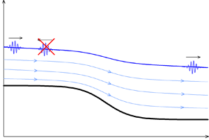
The conditions under which waves propagate in inhomogeneous media without reflection and scattering are of significant physical interest and are important for practical purposes. Under such conditions, wave energy can be most effectively transmitted over long distances. In a recent paper (Churilov & Stepanyants Reference Churilov and Stepanyants2022) we found two classes of shallow-water flows in channels with the variable width  $W(x)$ and bottom profile
  $z_B = B(x)$ (see figure 1) which provide reflectionless (RL) propagation of long surface waves. However, the profiles found in that paper do not exhaust all possible classes of flows that provide RL wave propagation. Recently, we found one more class of such flows which is noticeably different from those that have already been studied. The aim of this paper is to describe this specific class of flows and complete the description of all possible classes of RL flow, at least within the framework of the approach based on a factorisation of the wave equations (see below). Thus, this paper can be considered as the continuation of our previous paper (Churilov & Stepanyants Reference Churilov and Stepanyants2022).

Figure 1. Sketch of the flow configuration in the vertical plane.
2. Basic equations
In a stationary flow, the mass conservation,
 \begin{equation} U(x)H(x)W(x) = {\rm const.}, \end{equation}
together with the Bernoulli law,
 \begin{equation} \tfrac{1}{2}U^2(x) + g\left(H(x) + B(x)\right) = {\rm const.}, \end{equation}
provide independent variation along the longitudinal channel  $x$-axis the flow,
  $U(x)$, and wave,
  $c(x)=\sqrt {gH(x)}$, speeds (we assume that both of them are positive). Here,
  $H(x)$ is the water depth in the channel, and
  $g$ is the acceleration due to gravity.
In the shallow-water approximation, the linearised Euler equation,
 \begin{equation} \displaystyle\frac{\partial \tilde u}{\partial t} + \displaystyle\frac{\partial(U\tilde u)}{\partial x} ={-}g\displaystyle\frac{\partial\eta}{\partial x}, \end{equation}
where  $\tilde u(x,t)$ is the velocity perturbation and
  $\eta (x,t)$ is the deviation of the water surface from the equilibrium, and mass balance equation,
 \begin{equation} \displaystyle\frac{\partial\eta}{\partial t} + \displaystyle\frac{1}{W}\,\displaystyle\frac{\partial}{\partial x}\left[W(U\,\eta + H\,\tilde u)\right] \equiv \displaystyle\frac{\partial\eta}{\partial t} + HU\displaystyle\frac{\partial}{\partial x}\left(\displaystyle\frac{\eta}{H} + \displaystyle\frac{\tilde u}{U}\right) = 0, \end{equation}
can be reduced to a single equation in two ways.
On the one hand, we can introduce the velocity potential  $\varphi (x)$ by setting
  $\tilde{u}(x,t) = \partial \varphi (x,t)/\partial x$, expressing
  $\eta$ in terms of
  $\varphi (x)$ using (2.3) and substituting in (2.4). Then, we can present
  $\varphi$ in the form
  $\varphi (x, t) = a(x)\psi (x,t)$ and obtain an equation for
  $\psi$ in two equivalent forms (see Churilov & Stepanyants Reference Churilov and Stepanyants2022)
 $$\begin{align} &\left\{\displaystyle\frac{\partial}{\partial t} + \left[U(x) - c(x)\right]\,\displaystyle\frac{\partial}{\partial x} + U(x)\left(\displaystyle\frac{U'(x)}{U(x)} - \displaystyle\frac{c'(x)}{c(x)}\right)\right\} \left(\displaystyle\frac{\partial}{\partial t}+ \left[U(x)+c(x)\right]\displaystyle\frac{\partial}{\partial x}\right)\psi\nonumber\\ &\equiv \left\{\displaystyle\frac{\partial}{\partial t} + \left[U(x) + c(x)\right]\,\displaystyle\frac{\partial}{\partial x} + U(x)\left(\displaystyle\frac{U'(x)}{U(x)} - \displaystyle\frac{c'(x)}{c(x)}\right)\right\} \left(\displaystyle\frac{\partial}{\partial t}+ \left[U(x)-c(x)\right]\displaystyle\frac{\partial}{\partial x}\right)\psi \!=\! 0, \end{align}$$
(hereinafter the prime denotes the  $x$-derivative) provided that the following equations are fulfilled:
 \begin{equation} \displaystyle\frac{{\rm d} a}{{\rm d}\kern0.7pt x} = \displaystyle\frac{{\mathcal{B}}\,c^2U}{c^2-U^2} \quad \text{and} \quad a(x) = \left[c(x)\,U(x)\right]^{1/2}, \end{equation}
or, equivalently,
 \begin{equation} \displaystyle\frac{{\rm d}(c\,U)}{{\rm d}\kern0.7pt x} \equiv c(x)\displaystyle\frac{{\rm d} U}{{\rm d}\kern0.7pt x} + U(x) \displaystyle\frac{{\rm d} c}{{\rm d}\kern0.7pt x} = \displaystyle\frac{{\mathcal{B}}c^{5/2}(x)\,U^{3/2}(x)}{c^2(x)-U^2(x)}. \end{equation}
Here,  ${\mathcal {B}} = {\rm const.}$ (in Churilov & Stepanyants Reference Churilov and Stepanyants2022 it was denoted by
  $D$), and
  $c^{1/2}(x)$ and
  $U^{1/2}(x)$ should be considered as positive functions. The general solution of (2.5) is the sum of two independent waves of arbitrary shape travelling with different speeds,
 \begin{equation} \psi(x,t) = \psi_1\left(t-\int\displaystyle\frac{{\rm d}\kern0.7pt x}{U(x)+c(x)}\right) + \psi_2\left(t-\int\displaystyle\frac{{\rm d}\kern0.7pt x}{U(x)-c(x)}\right). \end{equation}
It is in (2.7), which specifies such a relationship between  $U(x)$ and
  $c(x)$, that the inhomogeneous flow becomes reflectonless.
On the other hand, we can introduce another potential,  $\phi$, by setting
  $W(x)\eta (x,t) = \partial \phi (x,t)/\partial x$. After integrating (2.4), expressing
  $\tilde{u}$ in terms of
  $\phi$ and substituting it into (2.3), we get the equation
 \begin{equation} \left(\displaystyle\frac{\partial}{\partial t}+U\displaystyle\frac{\partial}{\partial x}+2U'\right) \left(\displaystyle\frac{\partial\phi}{\partial t}+U\displaystyle\frac{\partial\phi}{\partial x}\right)= c^2W\displaystyle\frac{\partial}{\partial x}\left(\displaystyle\frac{1}{W}\displaystyle\frac{\partial\phi}{\partial x}\right). \end{equation}
Note that this equation is valid in the absence of flow as well. Now, we put  $\phi (x,t) = A(x)\chi (x,t)$, where
  $A(x) > 0$, eliminate
  $W$ using (2.1) and obtain
 $$\begin{align} &\displaystyle\frac{\partial^2\chi}{\partial t^2} + (U^2-c^2)\displaystyle\frac{\partial^2\chi}{\partial x^2} + 2U\displaystyle\frac{\partial^2\chi}{\partial t\partial x} + 2\left(U\displaystyle\frac{A'}{A} + U'\right)\displaystyle\frac{\partial\chi}{\partial t}\nonumber\\ &\quad +\left[2(U^2-c^2)\displaystyle\frac{A'}{A} - c^2\displaystyle\frac{U'}{U} + 3UU' - 2cc' \right]\displaystyle\frac{\partial\chi}{\partial x} + T(x)\chi = 0, \end{align}$$
where  $T(x)$ is defined through the equation
 \begin{equation} A(x)\,T(x) = (U^2-c^2)A'' + [3UU' - c^2(\ln U)' - 2cc']A'. \end{equation}
It can be readily shown that  $T(x) \equiv 0$ if
  $A(x)$ obeys the equation
 \begin{equation} \displaystyle\frac{{\rm d} A}{{\rm d}\kern0.7pt x} = \displaystyle\frac{{\mathcal{C}}}{U(x)[U^2(x) - c^2(x)]}, \quad {\mathcal{C}} = {\rm const.} \end{equation}
Following Churilov & Stepanyants (Reference Churilov and Stepanyants2022), consider the model equation
 \begin{equation} \left(\displaystyle\frac{\partial}{\partial t} + v_1(x)\displaystyle\frac{\partial}{\partial x} + {\mathcal{F}}(x)\right) \left(\displaystyle\frac{\partial}{\partial t} + v_2(x)\displaystyle\frac{\partial}{\partial x}\right){\mathcal{H}}(x,t) = 0. \end{equation}
At least one of its solutions has the form of a travelling wave,
 \begin{equation} {\mathcal{H}}(x,t) = {\mathcal{H}}_1\left(t - \int\displaystyle\frac{{\rm d}\kern0.7pt x}{v_2(x)}\right), \end{equation}
where  ${\mathcal {H}}_1(z)$ is an arbitrary function. Let us remove the brackets in (2.13)
 $$\begin{align} &\displaystyle\frac{\partial^2 \mathcal{H}}{\partial t^2} + v_1(x)v_2(x)\displaystyle\frac{\partial^2 \mathcal{H}}{\partial x^2} + \left[v_1(x) + v_2(x)\right]\displaystyle\frac{\partial^2 \mathcal{H}}{\partial t\partial x},\nonumber\\ &\quad + {\mathcal{F}}(x)\displaystyle\frac{\partial {\mathcal{H}}}{\partial t} + [v_1(x)v'_2(x) + {\mathcal{F}}(x)v_2(x)] \displaystyle\frac{\partial {\mathcal{H}}}{\partial x} = 0, \end{align}$$
and find conditions when this equation coincides with (2.10) provided that  $T(x)\equiv 0$. Then, we obtain
 \begin{gather} v_1(x)v_2(x) = U^2(x) - c^2(x), \quad v_1(x) + v_2(x) = 2U(x) , \end{gather}
 \begin{gather} {\mathcal{F}} = 2\left(U\displaystyle\frac{A'}{A} + U'\right), \quad v_1v'_2 + {\mathcal{F}} v_2 = 2(U^2-c^2)\displaystyle\frac{A'}{A} - c^2\displaystyle\frac{U'}{U}+3UU'-2cc'. \end{gather}
Equations (2.16a,b) are fulfilled if either  $v_1 = U - c$ and
  $v_2 = U + c$ or
  $v_1 = U + c$ and
  $v_2 = U - c$. In both these cases (2.17a,b) yields, up to an unimportant numerical factor,
 \begin{equation} A(x) = \left[c(x)U(x)\right]^{{-}1/2} \equiv a^{{-}1}(x). \end{equation}
With this in mind, (2.12) can be written as
 \begin{equation} \displaystyle\frac{{\rm d} A^{{-}1}}{{\rm d}\kern0.7pt x} \equiv \displaystyle\frac{{\rm d} a}{{\rm d}\kern0.7pt x} = \displaystyle\frac{{\mathcal{C}}\,c(x)}{c^2(x) - U^2(x)}, \quad \text{or} \quad \displaystyle\frac{{\rm d}(c\,U)}{{\rm d}\kern0.7pt x} = \displaystyle\frac{{\mathcal{C}}\,c^{3/2}(x)\,U^{1/2}(x)}{c^2(x) - U^2(x)}. \end{equation}
When (2.19) is fulfilled, the function  $\chi (x, t)$ obeys the same (2.5) as
  $\psi (x, t)$, and in the general case is also equal to the sum of two travelling waves of arbitrary shape,
 \begin{equation} \chi(x,t) = \chi_1\left(t-\int\displaystyle\frac{{\rm d}\kern0.7pt x}{U(x)+c(x)}\right) + \chi_2\left(t-\int\displaystyle\frac{{\rm d}\kern0.7pt x}{U(x)-c(x)}\right). \end{equation}
However, RL propagation of these two waves is now secured by (2.19), which differs from (2.7). The physical variables  $\tilde u$ and
  $\eta$ are related to
  $\phi$ and
  $\chi$ in the following way:
 \begin{equation} \left. \begin{aligned} \tilde u(x,t) & ={-}\displaystyle\frac{1}{H\,W}\left[\displaystyle\frac{\partial\phi}{\partial t} + U\displaystyle\frac{\partial\phi}{\partial x}\right] ={-}\displaystyle\frac{1}{HWa} \left[\displaystyle\frac{\partial\chi}{\partial t} + U\displaystyle\frac{\partial\chi}{\partial x} - \displaystyle\frac{a'}{a}U\chi(x,t)\right],\\ \eta(x,t) & = \displaystyle\frac{1}{W}\displaystyle\frac{\partial\phi}{\partial x} = \displaystyle\frac{1}{Wa} \left[\displaystyle\frac{\partial\chi}{\partial x} - \displaystyle\frac{a'}{a}\chi(x,t)\right]. \end{aligned} \right\} \end{equation}
 The problem of finding RL profiles  $c(x)$ and
  $U(x)$ is that there are an infinite number of solutions, since these two velocities are related by only one (2.7) or (2.19). To find specific solutions, it is necessary to set additionally either one of the speeds, or the relationship between them. Below we will assume that
  $c(x)$ is known. Other options (setting
  $U(x)$ or the functional relationship between the speeds) have been considered in the context of (2.7) by Churilov & Stepanyants (Reference Churilov and Stepanyants2022).
At first glance, the differences between (2.7) and (2.19) are insignificant, but the properties of the RL velocity profiles that satisfy them notably differ. Only when  ${\mathcal {B}} = {\mathcal {C}} = 0$ do both equations lead to the same relation between the velocities,
  $a(x) = \textrm {const.}$, or
 \begin{equation} c(x)\,U(x) = \varPi = {\rm const.} > 0. \end{equation}
In this class of RL flows (let us call it class A) the following relations are fulfilled owing to (2.22) and (2.1):
 \begin{equation} W(x)\,H^{1/2}(x) = {\rm const.} \quad \text{and} \quad U(x)\,H^{1/2}(x) = {\rm const.}, \end{equation}
so that  $U(x)/W(x) = \textrm {const.}$, i.e. the wider the channel, the higher the fluid velocity.
In studies of RL propagation of long surface waves in channels without a current, the relation (2.23b) plays an important role (see, for example, Pelinovsky et al. Reference Pelinovsky, Didenkulova, Shurgalina and Aseeva2017a; Pelinovsky, Didenkulova & Shurgalina Reference Pelinovsky, Didenkulova and Shurgalina2017b). It distinguishes the so-called self-consistent channels – the only class of channels with regular  $W (x)$ and
  $H(x)$ profiles, in which waves propagate without reflection along the entire
  $x$-axis. Class A contains RL flows in self-consistent channels with currents, and these flows are also regular. One can set the profile of one of the velocities (for example,
  $U(x)$) on the entire
  $x$-axis in the form of an arbitrary continuous positive function and, using (2.22), obtain a family of corresponding profiles for another velocity (
 $c(x)$) ‘labelled’ by the parameter
  $\varPi$.
The class of RL flows controlled by (2.7) with  ${\mathcal {B}} \ne 0$ (the B class of flows) has been studied in detail by Churilov & Stepanyants (Reference Churilov and Stepanyants2022). Below, we consider the C class of RL flows obeying equation (2.19) with
  ${\mathcal {C}} \ne 0$.
3. C-class RL flows
3.1. The distinctive features of C-class flows compared with B-class flows
The similarities and differences in the behaviour of C-class and B-class flows are determined by the similarities and differences between (2.19) and (2.7). Equation (2.7) is homogeneous in the velocities  $c$ and
  $U$, and the constant
  ${\mathcal {B}}$ has the dimension of inverse length, whereas (2.19) does not have this property, and
  ${\mathcal {C}}$ has the dimension of acceleration. Therefore, in the B class of flows one can introduce the dimensionless coordinate
  $\xi = {\mathcal {B}}\, x$ regardless of the velocity scale
  $c_0$, and in the C class, the dimensionless variables can be introduced only through the following scaling:
 \begin{equation} \tilde{\xi} = {\mathcal{C}}x/c^2_0, \quad \tilde{c} = c/c_0, \quad \tilde{U} = U/c_0, \quad \tilde{a} = a/c_0. \end{equation}
Omitting the tildes, we rewrite (2.19) in the dimensionless form
 \begin{equation} \displaystyle\frac{{\rm d}(cU)}{{\rm d}\xi} = \displaystyle\frac{2c^{3/2}(\xi)U^{1/2}(\xi)}{c^2(\xi) - U^2(\xi)}. \end{equation}
It should be noted that, due to the invariance of (2.19) with respect to the simultaneous replacement of  $x \to -x$ and
  ${\mathcal {C}} \to -{\mathcal {C}}$, the transition to the coordinate
  $\xi$ removes, to a certain extent, the distinction between the concepts of ‘upstream’ and ‘downstream.’ Indeed, if
  $c(x)$ and
  $U(x)$ satisfy (2.19) for
  ${\mathcal {C}} = {\mathcal {C}}_0$, then
  $c(-x)$ and
  $U(-x)$ satisfy the same equation for
  ${\mathcal {C}} = -{\mathcal {C}}_0$, however,
  $U(x) > 0$. For this reason, we will use the terms ‘to the left’ (‘to the right’) in the sense of ‘in the direction of decreasing (increasing) the coordinate
  $\xi$.’
The right-hand side of (3.2) is singular for  $U = c$,
  $U = 0$,
  $c = 0$ as well as for the unbounded growth of
  $U(\xi )$ and/or
  $c(\xi )$. To solve the question of whether these singularities are attainable at a finite
  $\xi$, we rewrite (2.19) in the form
 \begin{equation} \displaystyle\frac{{\rm d}}{{\rm d}\xi}\ln a(\xi) = \displaystyle\frac{c^{1/2}(\xi)} {U^{1/2}(\xi)\left[c^2(\xi) - U^2(\xi)\right]}. \end{equation}
It is easy to see that, if  $c(\xi )$ is bounded everywhere, i.e.
  $0 < c(\xi ) < \infty$, then not only can
  $U = c$ be reached at a finite
  $\xi$, as in the B class of flows, but also
  $U = 0$ can be reached at some other finite point
  $\xi$, whereas
  $U = \infty$ can be attained only asymptotically, when
  $\xi \to -\infty$. Similarly,
  $c = 0$ and
  $c = \infty$, are attainable only asymptotically.
For further consideration, it is convenient to introduce functions determined by the ratio of the velocities  $U(\xi )$ and
  $c(\xi )$ at each point
  $\xi$
$\xi$
 \begin{equation} F(\xi) = \left[\displaystyle\frac{U(\xi)}{c(\xi)}\right]^{1/2} \equiv \left[\displaystyle\frac{U^2(\xi)}{g H(\xi)}\right]^{1/4} \quad \text{and} \quad f(\xi) = \displaystyle\frac{1}{F(\xi)}. \end{equation}
For the sake of brevity, we will call function  $F(\xi )$ the Froude number, and function
  $f(\xi )$ the reciprocal Froude number (in Churilov & Stepanyants Reference Churilov and Stepanyants2022 they were denoted as
  $u(\xi )$ and
  $w(\xi )$). In terms of
  $F$ and
  $f$, (3.2) and (3.3) have the form
 $$\begin{gather} c^2(\xi)\displaystyle\frac{{\rm d} F}{{\rm d}\xi} = \displaystyle\frac{1}{1-F^4(\xi)} - M(\xi)F(\xi), \end{gather}$$
 $$\begin{gather}c^2(\xi)\displaystyle\frac{{\rm d} f}{{\rm d}\xi} = \displaystyle\frac{f^6(\xi)}{1-f^4(\xi)} + M(\xi)f(\xi), \end{gather}$$
 $$\begin{gather}c(\xi)\displaystyle\frac{{\rm d} a}{{\rm d}\xi} = \displaystyle\frac{1}{1 - F^4(\xi)} = \displaystyle\frac{f^4(\xi)}{f^4(\xi) - 1}, \end{gather}$$
where
 \begin{equation} M(\xi) = c(\xi)\displaystyle\frac{{\rm d} c}{{\rm d}\xi} \equiv \displaystyle\frac{{\rm d}}{{\rm d}\xi}\left(\displaystyle\frac{c^2(\xi)}{2}\right) \equiv \displaystyle\frac{g}{2}\displaystyle\frac{{\rm d} H(\xi)}{{\rm d}\xi} \end{equation}
is determined by the bottom slope. It is convenient to present solutions of these equations as a set of trajectories (the phase portrait) on the half-plane  $(\xi, F)$ or
  $(\xi, f)$ (recall that functions
  $F$ and
  $f$ are positive).
As a useful illustration, consider flows in channels of constant depth, where the wave velocity is also constant,  $c(\xi ) = c_0$. Setting
  $c_0 = 1$ and integrating (3.5), we arrive at the algebraic equation
 \begin{equation} F^5(\xi) - 5F(\xi) + 5(\xi - \xi_0) = 0, \quad \xi_0 = {\rm const.} \end{equation}
If  $\xi _0 < \xi \le \xi _* = \xi _0 + 4/5$, then this equation has two positive roots
  $F_\pm (\xi )$ which merge into one double root
  $F=1$ at
  $\xi = \xi _*$. In the vicinity of the point
  $\xi _*$ these solutions are
 \begin{equation} F_\pm(\xi) \approx 1 \pm\tfrac{1}{2}\left(\xi_*-\xi\right)^{1/2} - \tfrac{1}{4}\left(\xi_*-\xi\right) + \ldots . \end{equation}
The bigger root,  $F_+ \ge 1$, grows indefinitely when
  $\xi$ decreases from
  $\xi _*$ up to minus infinity, whereas the smaller root,
  $F_- \le 1$, changes its sign at
  $\xi = \xi _0$
 \begin{equation} F_-(\xi) = \xi - \xi_0 + \tfrac{1}{5}(\xi - \xi_0)^5 + \ldots, \end{equation}
so that, for  $\xi < \xi _0$, (3.9) has only a single positive root. Thus,
  $\xi _0$ is the singular point for subcritical flow in which
  $U(\xi )$ vanishes,
  $U(\xi ) \sim (\xi -\xi _0)^2$.
Thus, in channels of constant depth, subcritical flows of C class (as opposed to those of B class) remain RL only within a finite interval of  $\xi$,
  $\xi _0 < \xi < \xi _*$, and supercritical flows are RL on the semi-axis
  $\xi < \xi _*$ (see figure 2 and compare it with figure 3a in Churilov & Stepanyants Reference Churilov and Stepanyants2022). Let us find the conditions under which these restrictions are absent on some part of the trajectories.

Figure 2. Phase portrait of C-class flows in a channel of constant depth in subcritical ( $F < 1$) and supercritical (
 $F > 1$) regions.
3.2. Global trajectories and asymptotic behaviour
For a subcritical trajectory to be unbounded in  $\xi$, i.e. to be global, it must reach neither
  $F = 1$ when
  $\xi$ increases, nor
  $F = 0$ when
  $\xi$ decreases. Thus, the task is split into two parts. Let us find first the conditions under which a trajectory is not bounded from the right. As in the B-class flows, reaching the value
  $F = 1$ can only be prevented by the presence on the phase plane of regions with opposite signs of the right-hand side of (3.5), separated by the null-isocline (NI). NI is described by the equation
 \begin{equation} G(F_0) = F^5_0(\xi) - F_0(\xi) ={-}M^{{-}1}(\xi). \end{equation}
This equation has two positive roots,  $0 < F_{0-}(\xi ) \le F_{0+}(\xi ) < 1$ if (see figure 3a)
 \begin{equation} M(\xi) \ge M_c = \frac{5^{5/4}}{4} \approx 1.8692. \end{equation}


Thus, in the subcritical region, NI appears only at a sufficiently large slope of the channel bottom as a result of the merger of two complex conjugate roots of (3.12). NI has two branches that cannot extend far to the left. Indeed, if  $c(\xi _1) = c_1 > 0$ and
  $M(\xi ) \ge M_c$ for
  $\xi < \xi _1$ then, with decreasing
  $\xi$, we will inevitably arrive at the singularity
  $c = 0$ (
 $H = 0$) for a finite
  $\xi$.
Let us assume that  $M(\xi ) = M_c$ for
  $\xi = \xi _c$ and grows monotonically for
  $\xi > \xi _c$. Then NI branches,
  $F = F_{0\pm }(\xi )$, start at the point
  $\xi = \xi _c$ and each monotonically tends to its own limit (see figure 4). The slope of the trajectories is negative between the branches and positive outside. Therefore, trajectories passing above
  $F_{0+}(\xi )$ end up reaching
  $F = 1$ at finite
  $\xi$. But any trajectory that crosses any branch remains between them up to
  $\xi = +\infty$, i.e. is not bounded on the right, as well as all trajectories lying below it (see figure 4a).

Figure 4. The subcritical part of the phase portrait of (3.5) for  $M_0 = 3$. (a) NI (curve 1) and surrounding trajectories, bounded (curves 2–4) and unbounded (curves 5–8) on the right; trajectories 7 and 8 are bounded from the left by the singularity
  $F = 0$. (b) Bounded (curves 2–4 and 8) and global (curves 5–7) trajectories in the presence of a NI (curve 1) and with inequality (3.22) fulfilled; blue and red dashed lines show the boundaries of the bundle of global trajectories.
Monotonic growth of  $M(\xi )$ does not require so fast an increase in depth. In the borderline case, when
  $M(\xi )$ tends to the finite limit
  $M_0 > M_c$ when
  $\xi \to +\infty$,
 \begin{align} H(\xi)\sim M_0\xi, \quad F(\xi) \to F_{0-} > 0, \quad U(\xi) \approx F^2_{0-}c(\xi) \sim \xi^{1/2}, \quad W(\xi) \sim \xi^{{-}3/2}, \end{align}
that is, the flow and wave velocities grow in the same way, and the channel is narrowed.
As in the B class of flows, the asymptotic (for  $\xi \to \pm \infty$) behaviour of subcritical flows depends on the convergence at the upper limit of the integrals
 \begin{equation} I_{F\pm}(\xi) ={\pm}\displaystyle\int_{\xi}^{{\pm}\infty}\displaystyle\frac{{\rm d} y}{c(y)}. \end{equation}
The convergence requires that function  $c(\xi )$ must grow with
  $\xi$ faster than a linear function, for example, as
  $|\xi |^{1+\varepsilon }$, where
  $\varepsilon > 0$.
Let function  $M(\xi )$ grow unlimitedly, so that
  $F_{0-}(\xi ) \sim M^{-1}(\xi ) \to 0$. Consider a trajectory passing through the point
  $(\xi _1, \, F_1)$ into the region
  $\xi > \xi _1$, and denote
  $c_1 = c(\xi _1)$ and
  $a_1 = c_1F_1$. From (3.7) we find
 \begin{equation} a(\xi) = a_1 + \displaystyle\int_{\xi_1}^{\xi}\displaystyle\frac{{\rm d} y}{c(y)[1-F^4(y)]} = a_1 + \displaystyle\frac{1}{1-F^4(\xi_a)}\displaystyle\int_{\xi_1}^{\xi}\displaystyle\frac{{\rm d} y}{c(y)}, \end{equation}
where  $\xi _a$ lies between
  $\xi _1$ and
  $\xi$. If the integral
  $I_{F +}(\xi _1)$ converges, then
  $a(\xi )$ tends to the limiting value
  $a_{1+} > 0$, and the asymptotic relations hold (cf. (2.23))
 \begin{equation} W(\xi) \sim U(\xi) \sim F(\xi) \sim H^{{-}1/2}(\xi) \sim c^{{-}1}(\xi). \end{equation}
If  $c(\xi )$ grows slower than
  $\xi$, for example, as
  $\xi ^p$, where
  $1/2 \le p < 1$, then the integral
  $I_{F +}(\xi _1)$ diverges, and the following asymptotic relations are valid:
 \begin{align} a(\xi) \sim \xi^{1-p}, \quad F(\xi) \sim \xi^{1-2p}, \quad U(\xi) \sim \xi^{2-3p}, \quad W(\xi) \sim \xi^{p-2}, \quad H(\xi) \sim \xi^{2p}. \end{align}
For  $p = 1/2$ these relations reduce to (3.14a–d), and when
  $p < 1/2$, NI disappears, and all trajectories are bounded on the right.
Consider now the continuation of the trajectory passing through the point  $(\xi _1, F_c)$ to the left, into the region
  $\xi < \xi _1$. For
  $a(\xi )$ not to vanish (together with
  $F(\xi )$) at some finite
  $\xi$, the integral
  $I_{F-}(\xi _1)$ must converge, and
  $\lim _{\xi \to -\infty } a(\xi ) = a_{1-}$ must be positive. Since
  $M(\xi ) < 0$ and
  $F(\xi )$ grows monotonically, the following inequalities hold:
 \begin{equation} a_1 - \displaystyle\frac{I_{F-}(\xi_1)}{1-F^4_1} < a_{1-} < a_1 - I_{F-}(\xi_1). \end{equation}
For the unlimited continuation of the trajectory to the left, it is necessary that
 \begin{equation} a_1 \equiv c_1F_1 > I_{F-}(\xi_1). \end{equation}
Because  $\max \left [F(1-F^4)\right ] = M_c^{-1}$ at
  $F = F_c = 5^{-1/4}$, we obtain the condition
 \begin{equation} c_1 \ge M_cI_{F-}(\xi_1), \end{equation}
sufficient for the trajectory passing through the point  $(\xi _1, F_c)$ to continue with no limit to the left as well. Together with this trajectory, all the above-lying (with
  $F_1 > F_c$) and some part of the below-lying (with
  $F_1 < F_c$) trajectories also continue with no limit to the left. The condition (3.20) cuts off low-lying trajectories which inevitably reach
  $F = 0$ at some finite
  $\xi$ (curves 7 and 8 in figure 4a and curve 8 in figure 4b).
Thus, we see that, for the existence of global subcritical flows of C class, the channel depth  $H(\xi )$ must increase indefinitely both to the left (faster than
  $\xi ^2$), for the inequality
 \begin{equation} c(\xi_c) \ge M_cI_{F-}(\xi_c) \end{equation}
to be hold, and to the right (faster than  $M_c \xi$) to ensure the monotonic growth of
  $M(\xi )$ for
  $\xi > \xi _c$, which is necessary to maintain NI. When these conditions are met, the set of global trajectories forms a bundle of trajectories strung on the trajectory passing through the point
  $(\xi _c, F_c)$ (in figure 4b the bundle boundaries are shown by dashed lines). Note that, in the supercritical part of the phase portrait (
 $F > 1$), all trajectories are bounded on the right by the singularity
  $F = f = 1$, as in figure 2.
Global supercritical trajectories can arise if, to the right of some point  $\xi _m > -\infty$, function
  $c(\xi )$ decreases monotonically (i.e.
  $M(\xi ) < 0$) that leads to the appearance of NI
  $f = f_0(\xi )$, described, according to (3.6), by the equation
 \begin{equation} f^5_0(\xi) ={-}M(\xi)[1-f^4_0(\xi)]. \end{equation}
As seen in figure 3(b), for any  $M < 0$ there is one positive root
  $f_0 < 1$ such that
 $$\begin{gather} f_0(\xi) = \left[{-}M(\xi)\right]^{1/5} + \tfrac{1}{5}\,M(\xi) + O(|M|^{9/5}), \quad ({-}M)\ll 1, \end{gather}$$
 $$\begin{gather}f_0(\xi) = 1 + \tfrac{1}{4}\,M^{{-}1}(\xi) + O(M^{{-}2}), \quad ({-}M)\gg 1. \end{gather}$$
 The existence of global solutions and the asymptotic behaviour of  $f(\xi )$ depend on the convergence at the upper limit of integrals (cf. (3.15))
 \begin{equation} I_{f\pm}(\xi) ={\pm}\displaystyle\int_{\xi}^{{\pm}\infty} c^3(y)\,{\rm d} y . \end{equation}
For the trajectory passing through the point ( $\xi _2, f_2$), we write (3.7) in the form
 \begin{equation} c(\xi)\displaystyle\frac{{\rm d} a}{{\rm d}\xi} ={-}\displaystyle\frac{f^4(\xi)}{1-f^4(\xi)} ={-}\displaystyle\frac{c^4(\xi)}{a^4(\xi)[1-f^4(\xi)]}, \end{equation}
and integrate it
 \begin{align} a^5(\xi) \equiv \left[\displaystyle\frac{c(\xi)}{f(\xi)}\right]^5 = a^5(\xi_2) - 5\displaystyle\int_{\xi_2}^{\xi}\displaystyle\frac{c^3(y)\,{\rm d} y}{1-f^4(y)} = \left[\displaystyle\frac{c(\xi_2)}{f_2}\right]^5 - \displaystyle\frac{5}{1-f^4(\xi_b)}\displaystyle\int_{\xi_2}^{\xi}c^3(y)\,{\rm d} y, \end{align}
where the point  $\xi _b$ lies between
  $\xi _2$ and
  $\xi$. The trajectory will be global if the integral
  $I_{f+}(\xi _2)$ converges and
  $f_2$ is small enough for positiveness of the limit
  $a^5_{2+}$ of the right-hand side of (3.28) when
  $\xi \to +\infty$. Then
  $a(\xi ) \to a_{2+}$, and relations (3.17) are valid.
For  $\xi \to -\infty$, all trajectories are unlimited, but the behaviour of function
  $f(\xi )$ depends on the convergence of the integral
  $I_{f-}(x_2)$. If it converges,
  $a(\xi ) \to a_{2-} > 0$, and relations (3.17) hold. If it diverges and, for example,
  $c(\xi ) \sim (-\xi )^q$, where
  $-1/3 < q < 1/2$, then
 \begin{equation} \left. \begin{gathered} a(\xi) \sim (-\xi)^{(1+3q)/5}, \quad f(\xi) \sim (-\xi)^{(2q-1)/5},\\ U(\xi) \sim (-\xi)^{(2+q)/5}, \quad W(\xi) \sim (-\xi)^{-(2+11q)/5}. \end{gathered} \right\} \end{equation}
For  $q > 0$, we have
 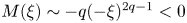 $M(\xi ) \sim -q(-\xi )^{2q-1} < 0$, and NI
  $f = f_0(\xi ) \approx M^{1/5}(\xi )$ appears, to which
  $f(\xi )$ tends asymptotically. And when
  $q \ge 1/2$, they both tend to a finite non-zero limit, so that, in this case for
  $\xi \to -\infty$, we have
 \begin{equation} a(\xi) \sim U(\xi) \sim c(\xi), \quad W(\xi) \sim c^{{-}3}(\xi), \quad H(\xi) \sim c^2(\xi). \end{equation}
 Let us describe in more detail the phase portrait of flows in a channel with the depth decreasing in such a manner that  $M(\xi ) < 0$ monotonically increases. Let
  $M(\xi )$ have a negative (finite or infinite) limit
  $M_-$ when
  $\xi \to -\infty$, whereas
  $M(\xi )$ goes to zero when
  $\xi \to +\infty$ faster than
  $-\xi ^{-5/3}$ to secure the existence of global trajectories. Then NI
  $f_0(\xi )$ decreases monotonically from
  $f_0(M_-)$ (see figure 3b) to zero. Each trajectory lying above NI or intersecting it is bounded on the right, but there are also global trajectories that lie entirely below NI and approach it from below as
  $\xi \to -\infty$ (see figure 5a).

Figure 5. Qualitative view of the phase portrait for  $M(\xi ) < 0$: (a) the supercritical part (
 $f < 1$,
  $f_0 (M_-) = 0.8$), line 1 is the NI; (b) the subcritical part (
 $F < 1$), the dashed line shows the separatrix.
Since  $M(\xi ) < 0$, in the subcritical part of the phase portrait (
 $f > 1$,
  $F < 1$) all trajectories are bounded on the right by the singularity
  $F = f = 1$. Suppose, however, that for some
  $\xi _1$ condition (3.21) is satisfied, so that there are trajectories that are unbounded from the left. From underlying trajectories, bounded on both sides, they are separated by a separatrix. For greater clarity, this part of the phase portrait is shown in figure 5(b) in coordinates
  $(\xi, F)$.
4. Concluding remarks
The C class of RL flows considered here is in many ways similar to the B class studied in Churilov & Stepanyants (Reference Churilov and Stepanyants2022). Indeed, in both of these classes flows can be either subcritical or supercritical, since, unlike flows of A class, the profiles  $c(\xi )$ and (or)
  $U(\xi )$ are inevitably singular in the critical point
  $U = c$. Flows passing through this point are, apparently, not RL. Further, supercritical flows of both classes are not bounded on the left in
  $\xi$, and their asymptotic behaviour and the existence of global flows are equally dependent on the behaviour of
  $c(\xi )$, namely, on the convergence of integrals (3.26).
The differences, and they are very significant ones, show subcritical currents. First of all, subcritical trajectories of the C class can be bounded in  $\xi$ not only from the right (by the critical point
  $U = c$), but also from the left by the singularity
  $U = 0$ (see figure 2 and compare with figure 3a in Churilov & Stepanyants Reference Churilov and Stepanyants2022). Further, the continuation of the trajectories to the right in both classes is possible only when a NI appears in the phase portrait. But the C class differs in both the geometry of NI (cf. NIs in figure 4 and figure 7 in Churilov & Stepanyants Reference Churilov and Stepanyants2022), and the need to exceed the threshold value (3.13) of the bottom slope for its appearance. Due to the
  $U$-shaped NI, there is no need for the convergence of the integral
  $I_{F+}(\xi )$ (see (3.15)) for the existence of trajectories that are not bounded on the right. Therefore, they appear with a slower increase in the depth of the channel
  $H(\xi )$ than in the B class, and differ in a variety of asymptotic behaviours, cf. (3.14a–d), (3.18a–e) and (3.17).
A separate question that does not arise in the B class but is important in the C class is the continuation of subcritical trajectories to the left. For this, the convergence of the integral  $I_{F-}(\xi )$ is not enough, and the more stringent inequalities (3.20) or (3.21) must hold. The simultaneous observance of the conditions for the unbounded continuation of the trajectory both to the right and to the left leads to the fact that, in the C class of flows, global trajectories form a bundle bounded by the Froude number
  $F$ both above and below (see figure 4b), whereas in the B class there is only an upper constraint (see figure 7 in Churilov & Stepanyants Reference Churilov and Stepanyants2022).
Funding
S.C. was financially supported by the Ministry of Science and Higher Education of the Russian Federation. Y.S. acknowledges the funding of this study provided by the grant No. FSWE-2020-0007 through the State task program in the sphere of scientific activity of the Ministry of Science and Higher Education of the Russian Federation, and grant No. NSH-70.2022.1.5 provided by the President of the Russian Federation for the State support of leading Scientific Schools of the Russian Federation.
Declaration of interests
The authors report no conflict of interest.
Author contributions
S.C. derived the theory. All authors contributed equally to analysing data, reaching conclusions and in writing the paper.


 Open access