2.1. Set-up

We consider a slender body placed in a fluid with a prescribed constant viscosity gradient

(2.1)\begin{equation} \eta({\boldsymbol{x}})=\eta_0\left(1+ \tilde{\boldsymbol{\kappa}}\boldsymbol{\cdot}\frac{\boldsymbol{x}-\boldsymbol{x}_0}{2a}\right). \end{equation}

Here, $\boldsymbol {x}_0$ represents the location at which the viscosity $\eta$ equals the reference viscosity $\eta _0$, and $\tilde {\boldsymbol {\kappa }}$ is the constant viscosity gradient, made dimensionless using $\eta _0$ and the body's half-length $a$. The fluid is subject to an incompressible external flow field denoted by $\boldsymbol {u}^{\infty }$. In the limit of vanishing Reynolds number, the total velocity field $\boldsymbol {u}$ satisfies the incompressible Stokes equations

(2.2)\begin{equation} \boldsymbol{\nabla} \boldsymbol{\cdot}\left\{\eta(\boldsymbol{x}) \left[\boldsymbol{\nabla} \boldsymbol{u}+(\boldsymbol{\nabla} \boldsymbol{u})^{\rm T}\right]\right\}= \boldsymbol{\nabla} p , \quad \boldsymbol{\nabla} \boldsymbol{\cdot} \boldsymbol{u}=0. \end{equation}

The slender body has half-length $a$ and a circular cross-section with maximum radius $b$, as illustrated in figure 1. The width-to-length aspect ratio of the body, $\varepsilon =b/a$, is assumed to be small. We parametrise the body using a dimensionless arc length $s$ running through its longitudinal centre (made dimensionless with respect to $a$). Under this parametrisation, the body's longitudinal centreline can thus be written as $a\,\tilde {\boldsymbol {R}}(s)$, where $-1\leq s\leq 1$, and its radius is described by $b\,\tilde {\lambda }(s)$. We assume that the dimensionless radius $\tilde {\lambda }(s)$ is continuous and that the radii at the endpoints of the body are zero (i.e. $\tilde {\lambda }(-1)=\tilde {\lambda }(1)=0$). Without loss of generality, we may set $\eta _0=\eta (a\,\tilde {\boldsymbol {R}}(s=0))$, i.e. we take the reference viscosity to be that at the instantaneous middle point of the filament. Unless otherwise stated, we carry out in what follows our derivation in a dimensionless form, non-dimensionalising all length scales by $a$, viscosity by $\eta _0$ (so that $\tilde \eta =\eta /\eta _0$), and velocity by a characteristic velocity $U$, with tilde signs used to represent the dimensionless variables.

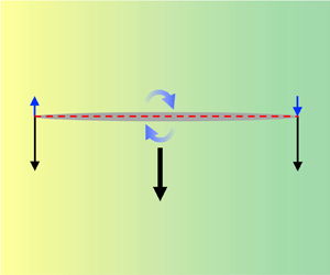
Figure 1. Sketch of a slender filament of length $2a$ and maximum radius $b$ in an external velocity field $\boldsymbol {u}^{\infty }$ in a fluid with a linearly varying viscosity $\eta ({\boldsymbol {x}})=\eta _0(1+\tilde {\boldsymbol {\kappa }}\boldsymbol {\cdot }(\boldsymbol {x}-\boldsymbol {x}_0)/(2a))$, where $\eta _0$ is the value of the viscosity at the instantaneous centre of the filament, and the constant viscosity gradient is denoted $\tilde {\boldsymbol {\kappa }}$. The red dashed line represents the body's centreline, located at $a\,\tilde {\boldsymbol {R}}(s)$, while the radius of the filament is denoted by $b\,\tilde {\lambda }(s)$. The gradient background represents the variation in viscosity schematically.

A classical approach used to compute the hydrodynamics of slender bodies in Stokes flows (Batchelor Reference Batchelor1970) is to approximate the velocity field $\boldsymbol {u}$ by a line distribution of point forces of density $\boldsymbol {f}$ over the centreline $a\,\tilde {\boldsymbol {R}}(s)$. The effects of the edges on the leading force distribution are assumed to be subdominant.

We introduce the Green's function $\boldsymbol{\mathsf{G}}^{V}\boldsymbol {\cdot }{\boldsymbol {f}}\,\text {d}\hat {s}/(8{\rm \pi} )$ to represent the velocity field produced by a force density $\boldsymbol {f}$ spread over an infinitesimal length $\text {d}\hat {s}$ in a viscous flow field with the prescribed viscosity field $\eta (\tilde {\boldsymbol {x}})$, where $\hat s$ is the dimensionless arc length integration variable. Since the viscosity field $\eta (\tilde {\boldsymbol {x}})$ is embedded into $\boldsymbol{\mathsf{G}}^{V}$, the Green's function has dimensions of the inverse of viscosity. Non-dimensionalising as ${\mathsf{G}}^{V}_{ij} \equiv \tilde{{\mathsf{G}}}^{V}_{ij}/\eta _0$, the flow created by a continuous force density $\boldsymbol {f}$ is written as

(2.3)\begin{equation} u_i(\boldsymbol{x})=\frac{1}{8{\rm \pi}\eta_0 }\int^1_{{-}1} \tilde{{\mathsf{G}}}^{V}_{ij}(\tilde{\boldsymbol{x}}-\tilde{\boldsymbol{R}}(\hat{s}))\,f_j(\hat{s}) \,\text{d}\hat{s}, \end{equation}

where, up to leading order in the viscosity gradient $\tilde {\boldsymbol {\kappa }}$, the Green's function is given by (Laumann & Zimmermann Reference Laumann and Zimmermann2019)

(2.4)\begin{equation} \tilde{{\mathsf{G}}}_{ij}^{V}(\boldsymbol{x}')=\frac{1}{\tilde{\eta}(\hat{s})}\left[\left(\frac{\delta_{ij}}{X}+\frac{x'_i x'_j}{X^3}\right)\left(1-\frac{\tilde{\kappa}_k x'_k}{4a\, \tilde{\eta}(\hat{s})}\right)+\frac{1}{4\tilde{\eta}(\hat{s})}\,\frac{x'_i\tilde{\kappa}_j - \tilde{\kappa}_i x'_j}{aX}\right], \quad X=|\boldsymbol{x}'|. \end{equation}

The objective is then to identify a suitable force density $\boldsymbol {f}$ so that (2.3) satisfies (2.2) along with the no-slip conditions $\boldsymbol {u}(s)=\boldsymbol {u}^{*}(s)$ along the surface of the body (where $\boldsymbol {u}^{*}(s)$ corresponds to the velocity averaged on the cross-section of the body).

The flow field in (2.3) is known to lead to a mathematical singularity if we model the filament as a line of vanishing thickness (Stokes paradox). To overcome this issue, the now-classical approach that leads to the results of RFT was proposed in the 1970s (Batchelor Reference Batchelor1970; Cox Reference Cox1970). The idea is to exploit the slenderness of the filament to match (2.3) at a point $s$ on the centreline to an inner flow field that corresponds to the flow around a cylinder of infinite extent and radius $b\, \tilde {\lambda }(s)$ that satisfies the uniform no-slip condition $\boldsymbol {u}(s)=\boldsymbol {u}^{*}(s)$ on its surface. The case of a uniform viscosity field ($\eta =\eta _0$) has been solved in classical work (Batchelor Reference Batchelor1970; Cox Reference Cox1970), and in this paper, we expand on these studies.

Specifically, we follow closely the derivation of Cox (Reference Cox1970) to obtain a solution for $\boldsymbol {f}$ that depends on the curved shape of the centreline in a constant viscosity gradient. In our derivation, we assume that the dimensionless viscosity gradient $\tilde {\boldsymbol {\kappa }}$ is small with respect to the spatial change in the length of the body. Since, as we see below, $\varepsilon$ needs to be exponentially small for RFT to be valid (meaning that $|\ln {\varepsilon }|$ is an asymptotically large number), it also follows that $|\tilde {\boldsymbol {\kappa }}| \gg \varepsilon$. Moreover, since any spatial deviation of the relative viscosity $\eta (a\,\tilde {\boldsymbol {R}})/(\eta _0 )$ along the radial direction away from the body's centreline (using the unit radial vector $\hat {\boldsymbol {e}}_{\rho }$ in local polar coordinates along the instantaneous centreline) is of the order of $(\tilde {\boldsymbol {\kappa }}\boldsymbol {\cdot }\hat {\boldsymbol {e}}_{\rho })\varepsilon$, the effects of a spatial change in the viscosity in the radial direction $\tilde {\boldsymbol {\kappa }}\boldsymbol {\cdot }\hat {\boldsymbol {e}}_{\rho }$ can be ignored to leading order in the body slenderness. The only relevant spatial component of the dimensionless viscosity gradient $\tilde {\boldsymbol {\kappa }}$ therefore acts in the tangential direction along the centreline itself, i.e. the component $\tilde {\kappa }_1=\tilde {\boldsymbol {\kappa }}\boldsymbol {\cdot }\hat {\boldsymbol {e}}_1$, where $\hat {\boldsymbol {e}}_1$ denotes the local unit vector directed in the tangent to the centreline.

We proceed in evaluating the force density $\boldsymbol {f}$ by computing the leading correction due to $\tilde {\kappa }_1$ to the inner flow field (§ 2.2) and the outer flow field for a uniform viscosity field (§ 2.3).

2.2. Inner solution

Following the calculation in Cox (Reference Cox1970), the inner solution $\tilde {\boldsymbol {u}}^{{in}}$ is found by focusing on an arbitrary point $s$ on the surface of the filament $s$ on the surface of the filament. Given that the filament is slender, on the relevant length scale $b$, we have $b\ll a$ and thus the filament appears locally to be a cylinder of circular cross-section and infinite extent, as sketched in figure 1. The radius of the cylinder is therefore approximately uniform. Using dimensionless polar coordinates $(\bar {\rho },\theta,\bar {x}_1)$, the surface of the cylinder $\bar {{\boldsymbol {x}}}$ can be parametrised using inner variables as

(2.5)\begin{equation} \bar{{\boldsymbol{x}}}=\bar{x}_1\,\hat{\boldsymbol{e}}_1 +\bar{\rho}\cos{\theta}\,\hat{\boldsymbol{e}}_2 +\bar{\rho}\sin{\theta}\,\hat{\boldsymbol{e}}_3, \quad \bar{\rho} =\tilde{\lambda}(s)+O(\varepsilon), \quad \bar{x}_1=s+O(\varepsilon), \end{equation}

about an orthogonal coordinate system with $\hat {\boldsymbol {e}}_1$, $\hat {\boldsymbol {e}}_2$ and $\hat {\boldsymbol {e}}_3$ directed in the direction of the tangent, normal and binormal of the centreline at $s$, respectively. Here, $\bar {(\cdot )}$ is used to denote the inner (dimensionless) variables, and we use $\tilde {(\cdot )}$ for the outer (dimensionless) variables. The inner flow $\tilde {\boldsymbol {u}}^{{in}}$ must satisfy (2.2) with the no-slip boundary conditions on the body surface, i.e. 

(2.6)\begin{equation} \tilde{\boldsymbol{u}}^{{in}}(\bar{\boldsymbol{x}})=\tilde{\boldsymbol{u}}^{*}(s). \end{equation}

We wish to solve the inner solution up to the leading order correction in $\tilde {\kappa }_1$ for a varying viscosity gradient. We thus solve for the velocity and pressure fields as expansions $\tilde {\boldsymbol {u}}^{{in}}=\tilde {\boldsymbol {u}}_0^{{in}}(\tilde {\kappa }_1)+O(\varepsilon )$ and $\tilde {p}^{{in}}=\tilde {p}_0^{{in}}(\tilde {\kappa }_1)+O(\varepsilon )$.

At the inner scale, the spatial change in the viscosity at a point $\bar {\boldsymbol {x}}$ on the surface is of the order of $\tilde {\kappa }_1(\bar {x}_1-s) \sim O(\tilde {\kappa }_1 \varepsilon )$. Therefore, the leading-order correction to $\tilde {\boldsymbol {u}}^{{in}}$ due to the viscosity change $\tilde {\boldsymbol {\kappa }}$ is asymptotically smaller than the zeroth-order solution for $\tilde {\boldsymbol {u}}_0^{{in}}$ in a uniform viscosity field with dimensionless viscosity taken to be $\tilde {\eta }_{s}\equiv \tilde {\eta }(\tilde {\boldsymbol {R}}(s))$ at each point along the centreline. The leading-order solution for $\tilde {\boldsymbol {u}}^{{in}}$ in both $\varepsilon$ and $\tilde {\boldsymbol {\kappa }}$ is thus exactly the same as that derived by Cox (Reference Cox1970) but with $\tilde {\eta }_0$ (which is equal to unity) formally interchanged with $\tilde {\eta }_{s}$.

Re-writing the expression for $\tilde {\boldsymbol {u}}^{{in}}$ using the outer variables $\tilde {\rho }=\varepsilon \bar {\rho }$ and $\tilde {x}=\varepsilon \bar {x}$ gives the inner boundary condition on the outer flow field $\tilde {\boldsymbol {u}}$ in the inner limit $\tilde {\rho }\to 0$, up to leading order in $\varepsilon$ and $\tilde {\kappa }_1$:

(2.7) \begin{gather} \left. \begin{gathered} \tilde{u}_z= E(\varepsilon) \ln(\tilde{\rho}/\tilde{\lambda})+\tilde{u}^{*}_{1}, \\ \tilde{u}_{\tilde{\rho}}= \tilde{u}^{*}_{2}\cos{\theta}+\tilde{u}^{*}_{3}\sin{\theta}+ (1-\tilde{\lambda}^2\tilde{\rho}^{{-}2}-2 \ln(\tilde{\rho}/\tilde{\lambda}))(C(\varepsilon)\cos{\theta} +D(\varepsilon)\sin{\theta} ), \\ \tilde{u}_{\theta}={-}\tilde{u}^{*}_{2}\sin{\theta}+\tilde{u}^{*}_{3}\cos{\theta}+ ({-}1+\tilde{\lambda}^2\tilde{\rho}^{{-}2}-2 \ln(\tilde{\rho}/\tilde{\lambda}))(D(\varepsilon)\cos{\theta}-C(\varepsilon)\sin{\theta} ), \\ \tilde{p}= \frac{4}{\tilde{\rho}}\left(C(\varepsilon)\cos{\theta}+D(\varepsilon)\sin{\theta}\right)+F(\varepsilon). \end{gathered} \right\} \end{gather}

Here, $C$, $D$, $E$ and $F$ are dimensionless coefficients that depend on $\varepsilon$, still to be determined.

2.3. Outer solution and matching

The calculation of the outer solution, and the matching with the inner solution, is computed analogously to Cox (Reference Cox1970). The method requires first expanding the coefficients $C$, $D$, $E$ and $F$ from (2.7) to leading order in $1/\ln {\varepsilon }$, and then equating each order of the expansion to the outer flow and pressure field. The expansion of the outer flow field to $O((\ln {\varepsilon })^{-1})$ is written formally as

(2.8)\begin{equation} \tilde{\boldsymbol{u}}= \tilde{\boldsymbol{u}}^{\infty}+ \tilde{\boldsymbol{u}}^{(1)}/\ln{\varepsilon}. \end{equation}

The leading-order terms in (2.7) are first equated with the leading-order velocity $\tilde{\boldsymbol {u}}^{\infty } -\tilde{\boldsymbol {u}}^{*}$. At $O((\ln {\varepsilon })^{-1})$, the outer flow field at the point at $\tilde {\boldsymbol {R}}(s)$ corresponds to the leading distribution of point forces as $\varepsilon \to 0$. Matching (2.7) to a line distribution of dimensionless point forces on $\tilde {\boldsymbol {R}}(s)$ with density $\tilde {\boldsymbol {f}}(s)$ as $\tilde {\rho }\to 0$ requires the outer force density to be (Cox Reference Cox1970)

(2.9)\begin{equation} \tilde{\boldsymbol{f}}(s)=4{\rm \pi}\,\tilde{\eta}_{s} (\tilde{\boldsymbol{u}}^{\infty}(\tilde{\boldsymbol{R}})-\tilde{\boldsymbol{u}}^{*}(s))\boldsymbol{\cdot} \left(\boldsymbol{I}-\frac{1}{2}\,\frac{\text{d}\tilde{\boldsymbol{R}}}{\text{d} s}\,\frac{\text{d}\tilde{\boldsymbol{R}}}{\text{d} s}\right). \end{equation}

Here, we have assumed that $\hat {\boldsymbol {e}}_2$ lies in the same plane as $\hat {\boldsymbol {e}}_1$ and $\tilde {\boldsymbol {u}}^{\infty }(\tilde {\boldsymbol {R}})-\tilde {\boldsymbol {u}}^{*}(s)$, so that the unit vectors $\hat {\boldsymbol {e}}_1, \hat {\boldsymbol {e}}_2, \hat {\boldsymbol {e}}_3$ can be expressed in terms of $\tilde {\boldsymbol {u}}^{\infty }(\tilde {\boldsymbol {R}})-\tilde {\boldsymbol {u}}^{*}(s)$ and $\textrm {d} \tilde {\boldsymbol {R}}(s)/ \textrm {d} s$ (Cox Reference Cox1970).

The flow field $\tilde {\boldsymbol {u}}^{(1)}$ can then be obtained as that produced by the distribution of point forces with density $\tilde {\boldsymbol {f}}$ to leading order, analogously to (2.3). It is thus written as

(2.10)\begin{equation} \tilde{u}^{(1)}_i=\lim_{\tilde{\rho}\to 0}\frac{1}{2}\int_{{-}1}^{1} \tilde{{\mathsf{G}}}^{V}_{ij}\left(\tilde{\boldsymbol{x}}'\right)\tilde{f}_{j}(\hat{s}) \,\text{d}\hat{s} , \quad \tilde{\boldsymbol{x}}'=\tilde{\boldsymbol{x}}(s)-\tilde{\boldsymbol{x}}(\hat{s}). \end{equation}

The only (but important) difference from the Cox (Reference Cox1970) derivation is with the definition of the tensor $\tilde {\boldsymbol{\mathsf{G}}}^V$, where here $\tilde {\boldsymbol{\mathsf{G}}}^V$ accounts for the prescribed viscosity gradient $\tilde {\boldsymbol {\kappa }}$, as given in (2.4).

Since we are interested in only the leading-order terms in $\varepsilon$, we can simplify the tensor $\tilde{{\mathsf{G}}}_{ij}^{V}$ in (2.10) further by noting that in the spatial region of the integrand, we have $1/\tilde {\eta }(\hat {s}) \approx (1/\tilde {\eta }_s)(1+\tilde {\boldsymbol {\kappa }}\boldsymbol {\cdot }(\tilde {\boldsymbol {x}}'/2))$. Under this assumption, the tensor in (2.4) becomes, to leading order in $\tilde {\boldsymbol {\kappa }}$ and $\varepsilon$,

(2.11)\begin{equation} \tilde{{\mathsf{G}}}_{ij}^{V}(\boldsymbol{x}')=\frac{1}{\tilde{\eta}_s}\left[\left(\frac{\delta_{ij}}{X'}+\frac{x'_i x'_j}{X'^3}\right)\left(1+\frac{\tilde{\kappa}_k x'_k}{4a }\right)+\frac{1}{4 }\,\frac{x'_i \tilde{\kappa}_j - \tilde{\kappa}_i x'_j}{aX'}\right] +O(\tilde{\boldsymbol{\kappa}}^2,\varepsilon). \end{equation}

To evaluate the flow from (2.10), we let $\tilde {\boldsymbol {u}}^{(1)}=\boldsymbol {J}^{*}+\boldsymbol {J}$, where $\boldsymbol {J}^{*}$ denotes the integral over the singular part of the integrand in (2.10) taken over the region $[s-\epsilon,s+\epsilon ]$ (where $\epsilon$ is an arbitrary number such that $\epsilon \ll 1$), and $\boldsymbol {J}$ is the integral on the remaining part of the line. Since $\epsilon \ll 1$, $\boldsymbol {J}^{*}$ can be evaluated analytically in the singular region of the integral as

(2.12)\begin{equation} J^{*}_i= \lim_{\tilde{\rho}\to 0}\frac{\tilde{\eta}_s}{2}(\tilde{u}^{\infty}_k(\hat{R})-\tilde{u}^{*}_k(s))\left(\delta_{jk}-\frac{1}{2}\,\frac{\text{d}\tilde{R}_j}{\text{d} s}\,\frac{\text{d}\tilde{R}_k}{\text{d} s}\right) \int_{s-\epsilon}^{s+\epsilon} \tilde{{\mathsf{G}}}^{V}_{ij}\left(\tilde{\boldsymbol{x}}'\right) \text{d}\hat{s}. \end{equation}

We can further simplify $\tilde {\boldsymbol{\mathsf{G}}}^V$ in this singular region. Since $\tilde {\boldsymbol {x}}(\hat {s}) \approx \hat {s} \hat {\boldsymbol {e}}_1$, we have $\tilde {\boldsymbol {x}}(s)=(s,\tilde {\rho } \cos {\theta },\tilde {\rho } \sin {\theta })$ and $\tilde {\boldsymbol {x}}(\hat {s})=(\hat {s},\tilde {\rho } \cos {\theta },\tilde {\rho } \sin {\theta })$. Recalling that the only contribution in $\tilde {\boldsymbol {\kappa }}$ with terms of order greater than $\varepsilon$ comes from $\tilde {\boldsymbol {\kappa }} \boldsymbol {\cdot }{\hat {\boldsymbol {e}}_1}=\tilde {\kappa }_1$, we obtain

(2.13)\begin{equation} \tilde{{\mathsf{G}}}_{ij}^{V}(\boldsymbol{x}')=\frac{1}{\tilde{\eta}_s}\left[\left(\frac{\delta_{ij}}{X'}+\frac{x'_i x'_j}{X'^3}\right)\left(1+\frac{\tilde{\kappa}_1 x'_1}{4a }\right)+\frac{1}{4 }\,\frac{x'_i \tilde{\kappa}_j \delta_{1j} - \tilde{\kappa}_i x'_j\delta_{1i}}{aX'}\right]+O(\tilde{\boldsymbol{\kappa}}^2,\varepsilon). \end{equation}

The integral in (2.12) can be evaluated analytically by introducing

(2.14)\begin{equation} {\mathsf{M}}_{ij}^{*}=\lim_{\tilde{\rho} \to 0} \int_{s-\epsilon}^{s+\epsilon} \tilde{{\mathsf{G}}}^{V}_{ij}\left(\tilde{\boldsymbol{x}}'\right) \text{d}\hat{s}, \end{equation}

with

(2.15)$$\begin{gather} {\mathsf{M}}_{xx}^{*}=\frac{1}{\tilde{\eta}_s}\left(4\ln\left(\frac{2\epsilon}{\tilde{\rho}}\right)-2\right) +O(\varepsilon\tilde{\boldsymbol{\kappa}},\varepsilon), \end{gather}$$

(2.16)$$\begin{gather}{\mathsf{M}}_{yy}^{*}=\frac{1}{\tilde{\eta}_s}\left(2\ln\left(\frac{2\epsilon}{\tilde{\rho}}\right) +2\cos^{2}{\theta}\right) +O(\varepsilon\tilde{\boldsymbol{\kappa}},\varepsilon), \end{gather}$$

(2.17)$$\begin{gather}{\mathsf{M}}_{zz}^{*}=\frac{1}{\tilde{\eta}_s}\left(2\ln\left(\frac{2\epsilon}{\tilde{\rho}}\right) +2\sin^{2}{\theta}\right) +O(\varepsilon\tilde{\boldsymbol{\kappa}},\varepsilon), \end{gather}$$

(2.18)$$\begin{gather}{\mathsf{M}}_{yz}^{*}={\mathsf{M}}_{zy}^{*}= \frac{2}{\tilde{\eta}_s}\sin{\theta}\cos{\theta}+O(\varepsilon\tilde{\boldsymbol{\kappa}},\varepsilon), \end{gather}$$

(2.19)$$\begin{gather}{\mathsf{M}}_{xy}^{*}={\mathsf{M}}_{yx}^{*}= O(\varepsilon\tilde{\boldsymbol{\kappa}},\varepsilon), \end{gather}$$

(2.20)$$\begin{gather}{\mathsf{M}}_{xz}^{*}={\mathsf{M}}_{zx}^{*}= O(\varepsilon\tilde{\boldsymbol{\kappa}},\varepsilon). \end{gather}$$

It is important to note that all integrated terms containing $\tilde {\kappa }_1$ either vanish over the region $[s-\epsilon,s+\epsilon ]$, or are of the order $O(\varepsilon \tilde {\kappa }_1)$. Therefore, $\boldsymbol {J}^{*}$ is the same as for the classical case of a constant viscosity up to order $O(\varepsilon \tilde {\boldsymbol {\kappa }},\varepsilon )$, but with the addition of the prefactor $1/\tilde {\eta }_s$ for the varying viscosity.

Since the leading-order contribution of $\tilde {\kappa }_1$ enters only in the non-singular part of the integral, $\boldsymbol {J}$, the dimensionless outer flow $\tilde {\boldsymbol {u}}^{(1)}$, pressure $\tilde {p}^{(1)}$ and force density $\bar {\boldsymbol {f}}(s)$ can be expressed in the same way as in Cox (Reference Cox1970) for a uniform viscosity field. Namely, equating (2.7)–(2.8) for $\tilde {\rho }\to 0$, one obtains the coefficients in (2.7) to be

(2.21)$$\begin{gather} C(\varepsilon ) = \frac{1}{\ln{\varepsilon}}\,\frac{1}{2}\,(\tilde{u}^{\infty}_{2}-\tilde{u}^{*}_{2})+ \frac{1}{(\ln{\varepsilon})^2}\,\frac{1}{4}\,(\tilde{u}^{\infty}_{2}-\tilde{u}^{*}_{2})\left(1+2\ln{\left(\frac{2\epsilon}{\tilde{\lambda}}\right)}+J_{2}\right) \nonumber\\ +\,O((\ln{\varepsilon})^{{-}3},\tilde{\boldsymbol{\kappa}} \varepsilon (\ln{\varepsilon})^{{-}1}), \end{gather}$$

(2.22)$$\begin{gather}D(\varepsilon )= \frac{1}{(\ln{\varepsilon})^2}\,\frac{J_{3}}{2}+O((\ln{\varepsilon})^{{-}3},\tilde{\boldsymbol{\kappa}} \varepsilon (\ln{\varepsilon})^{{-}1}) , \end{gather}$$

(2.23)$$\begin{gather}E(\varepsilon )={-}\frac{1}{\ln{\varepsilon}}\,(\tilde{u}^{\infty}_{1}-\tilde{u}^{*}_{1})+ \frac{1}{(\ln{\varepsilon})^2}\,\frac{1}{2}\,(\tilde{u}^{\infty}_{1}-\tilde{u}^{*}_{1})\left(1-2\ln{\left(\frac{2\epsilon}{\tilde{\lambda}}\right)}-J_{1}\right) \nonumber\\ +\,O((\ln{\varepsilon})^{{-}3},\tilde{\boldsymbol{\kappa}} \varepsilon (\ln{\varepsilon})^{{-}1}) . \end{gather}$$

The integral $\boldsymbol {J}$ is defined as

(2.24)\begin{align} J_i= \lim_{\epsilon\to 0}\frac{\tilde{\eta}_s}{2}\left[\int_{{-}1}^{s-\epsilon}+\int_{s+\epsilon}^{1}\right] \tilde{{\mathsf{G}}}^{V}_{ij}\left(\tilde{\boldsymbol{x}}(s)-\tilde{\boldsymbol{x}}(\hat{s})\right)\left(\delta_{jk}-\frac{1}{2}\,\frac{\text{d}\hat{R}_j}{\text{d} \hat{s}}\,\frac{\text{d}\hat{R}_k}{\text{d} \hat{s}} \right)\left(\tilde{u}^{\infty}_k(\hat{R})-\tilde{u}^{*}_k(\hat{s})\right) \text{d}\hat{s}, \end{align}

where $\hat {R}_i=\tilde {R}_i(\hat {s})$.

2.4. Force distribution

As shown by Cox (Reference Cox1970), the force distribution can be evaluated explicitly from (2.7) and (2.21)–(2.23) to give

(2.25)$$\begin{gather} \bar{\boldsymbol{f}}(s)=2{\rm \pi}\,\tilde{\eta}_s(\tilde{\boldsymbol{\kappa}}) \left[\frac{\tilde{\boldsymbol{u}}^{\infty}-\tilde{\boldsymbol{u}}^{*}}{\ln{\varepsilon}}+\frac{\boldsymbol{J}(\tilde{\boldsymbol{\kappa}})+(\tilde{\boldsymbol{u}}^{\infty}-\tilde{\boldsymbol{u}}^{*})\ln{(2\epsilon/\tilde{\lambda})}}{(\ln{\varepsilon})^2}\right]\boldsymbol{\cdot}\left[\frac{\text{d}\tilde{\boldsymbol{R}}}{\text{d} s}\,\frac{\text{d}\tilde{\boldsymbol{R}}}{\text{d} s}-2\boldsymbol{I}\right] \nonumber\\ {}+ \frac{\tilde{\boldsymbol{u}}^{\infty}-\tilde{\boldsymbol{u}}^{*}}{2(\ln{\varepsilon})^2}\boldsymbol{\cdot}\left[3\,\frac{\text{d}\tilde{\boldsymbol{R}}}{\text{d} s}\,\frac{\text{d}\tilde{\boldsymbol{R}}}{\text{d} s}-2\boldsymbol{I}\right]+O((\ln{\varepsilon})^{{-}3},\tilde{\boldsymbol{\kappa}} \varepsilon (\ln{\varepsilon})^{{-}1}). \end{gather}$$

Crucially, the only differences between our results and the derivation from Cox (Reference Cox1970) are that the correction due to the viscosity gradient $\tilde {\boldsymbol {\kappa }}$ enters through $\tilde {\eta }_s(\tilde {\boldsymbol {\kappa }})$ and $\boldsymbol {J}(\tilde {\boldsymbol {\kappa }})$.

Finally, with the knowledge of $\bar {\boldsymbol {f}}(s)$ in (2.25), the total hydrodynamic force $\boldsymbol {F}$, torque $\boldsymbol {T}$ and stresslet $\boldsymbol{\mathsf{S}}$ are

(2.26)$$\begin{gather} {F}_{i}=a\eta_0 U\int^{1}_{{-}1} \bar{f}_i(s) \,\text{d}s, \end{gather}$$

(2.27)$$\begin{gather}{T}_i=a^2\eta_0 U\int^{1}_{{-}1} [\tilde{\boldsymbol{R}}(s)\times \bar{\boldsymbol{f}}(s)]_i \,\text{d}s, \end{gather}$$

(2.28)$$\begin{gather}{\mathsf{S}}_{ij}=a^2\eta_0 U\int^{1}_{{-}1} \tilde{R}_i(s)\,\bar{f}_j(s)+ \tilde{R}_j(s)\,\bar{f}_i(s)]\,\text{d}s, \end{gather}$$

where in the expression for $\boldsymbol{\mathsf{S}}$, we have assumed that the centreline of the slender body is not deforming with time.

3.1. Uniform flow field

We begin here by focusing on a straight filament of length $2a$, which is held fixed in a uniform flow field $\boldsymbol {u}^{\infty }=U_1\hat {\boldsymbol {e}}_1+U_2\hat {\boldsymbol {e}}_2$ with constant viscosity gradient $\tilde {\boldsymbol {\kappa }}$. Without loss of generality, we may assume that the filament is held fixed with $\tilde {\boldsymbol {R}}(s)=s\hat {\boldsymbol {e}}_1$, hence $\textrm {d} \tilde {\boldsymbol {R}}/ \textrm {d} s =\hat {\boldsymbol {e}}_1$.

3.1.1. Computation of forces and torques

Under this parametrisation, (2.24) becomes

(3.1)\begin{equation} J_i=\frac{\tilde{\eta}_s}{2}\left[\int_{{-}1}^{s-\epsilon}+\int_{s+\epsilon}^{1}\right]\tilde{{\mathsf{G}}}^{V}_{ij}\left(s-\hat{s},0,0\right)\left(\frac{\tilde{U}_1}{2}\, \delta_{j1}+\tilde{U}_2\,\delta_{j2} \right)\text{d}\hat{s}. \end{equation}

Here, we have dimensionalised $U_1$ and $U_2$ by a typical speed $U$. This integral can be evaluated analytically using

(3.2)\begin{equation} {\mathsf{M}}_{ij}= \left[\int_{{-}1}^{s-\epsilon}+\int_{s+\epsilon}^{1}\right] \tilde{{\mathsf{G}}}^{V}_{ij}\left(s-\hat{s},0,0\right) \text{d}\hat{s}, \end{equation}

and its components are

(3.3)$$\begin{gather} {\mathsf{M}}_{xx}=\frac{2}{\tilde{\eta}_s}\left(\ln(1-s^2)-2\ln{\epsilon} +\frac{\tilde{\kappa}_1}{2}\,s \right) +O(\varepsilon\tilde{\boldsymbol{\kappa}},\varepsilon), \end{gather}$$

(3.4)$$\begin{gather}{\mathsf{M}}_{yy}=\frac{1}{\tilde{\eta}_s}\left(\ln(1-s^2)-2\ln{\epsilon} +\frac{\tilde{\kappa}_1}{2}\,s \right) +O(\varepsilon\tilde{\boldsymbol{\kappa}},\varepsilon), \end{gather}$$

(3.5)$$\begin{gather}{\mathsf{M}}_{zz}=\frac{1}{\tilde{\eta}_s}\left(\ln(1-s^2)-2\ln{\epsilon} +\frac{\tilde{\kappa}_1}{2}\,s \right) +O(\varepsilon\tilde{\boldsymbol{\kappa}},\varepsilon), \end{gather}$$

(3.6)$$\begin{gather}{\mathsf{M}}_{yz}={\mathsf{M}}_{zy}= O(\varepsilon\tilde{\boldsymbol{\kappa}},\varepsilon), \end{gather}$$

(3.7)$$\begin{gather}{\mathsf{M}}_{xy}={\mathsf{M}}_{yx}= O(\varepsilon\tilde{\boldsymbol{\kappa}},\varepsilon), \end{gather}$$

(3.8)$$\begin{gather}{\mathsf{M}}_{xz}={\mathsf{M}}_{zx}= O(\varepsilon\tilde{\boldsymbol{\kappa}},\varepsilon). \end{gather}$$

The integral in (3.1) then becomes

(3.9)\begin{equation} J_i=\frac{\tilde{U}_1\delta_{i1}+\tilde{U}_2\delta_{i2}}{4}(2\ln(1-s^2)-4\ln{\epsilon} +\tilde{\kappa}_1 s) +O(\varepsilon\tilde{\boldsymbol{\kappa}},\varepsilon). \end{equation}

Substituting (3.9) into (2.25) allows us to compute the components of the hydrodynamic force density as

(3.10)$$\begin{align} \bar{f}_1&=2{\rm \pi} \tilde{U}_1\tilde{\eta}_s \left[-\frac{1}{\ln{\varepsilon}}+\frac{1}{2(\ln{\varepsilon})^2}\left(1-2\ln{2}-\ln\left(\frac{1-s^2}{\tilde{\lambda}^2}\right)-s\,\frac{\tilde{\kappa}_1}{2}\right)\right]\nonumber\\ &\quad +O((\ln{\varepsilon})^{{-}3},\tilde{\boldsymbol{\kappa}} \varepsilon (\ln{\varepsilon})^{{-}1}), \end{align}$$

(3.11)$$\begin{align}\bar{f}_2&=2{\rm \pi} \tilde{U}_2\tilde{\eta}_s\left[-\frac{2}{\ln{\varepsilon}}+\frac{1}{(\ln{\varepsilon})^2}\left({-}1-2\ln{2}-\ln\left(\frac{1-s^2}{\tilde{\lambda}^2}\right)-s\,\frac{\tilde{\kappa}_1}{2}\right)\right]\nonumber\\ &\quad +O((\ln{\varepsilon})^{{-}3},\tilde{\boldsymbol{\kappa}} \varepsilon (\ln{\varepsilon})^{{-}1}). \end{align}$$

Evaluating the total force and torque in (2.26) and (2.27) requires integrating terms containing $\tilde {\eta }_s(s)=1+s\tilde {\kappa }_1/2$. Writing the total force $\boldsymbol {F}$ and torque $\boldsymbol {T}$ as asymptotic expansions, we have

(3.12)$$\begin{gather} F_i=F_i^{(0)}+\tilde{\kappa}_1 F_i^{(1)}+O(\tilde{\kappa}^2_1,\varepsilon\tilde{\kappa}_2, \varepsilon\tilde{\kappa}_3), \end{gather}$$

(3.13)$$\begin{gather}T_i=T_i^{(0)} +\tilde{\kappa}_1 T_i^{(1)}+O(\tilde{\kappa}^2_1,\varepsilon\tilde{\kappa}_2, \varepsilon\tilde{\kappa}_3). \end{gather}$$

The terms proportional to $U_1$ are, to leading order in $O((\ln {\varepsilon })^{-2})$, given by

(3.14)$$\begin{gather} F^{(0)}_1=a\eta_0 U_1\left[\frac{4{\rm \pi} }{\ln(2a/b)+C_1} \right], \quad C_1={-}\frac{1}{2}+\frac{1}{4}\int^{1}_{{-}1} \ln\left(\frac{1-s^2}{\tilde{\lambda}^2}\right) \text{d} s, \end{gather}$$

(3.15)$$\begin{gather}F^{(1)}_1= a\eta_0 U_1\left[-\frac{\rm \pi}{2(\ln{(b/a)})^2} \int^{1}_{{-}1} s\ln\left(\frac{1-s^2}{\tilde{\lambda}^2}\right) \text{d} s\right] , \end{gather}$$

(3.16)$$\begin{gather}T^{(0)}_2 = 0, \end{gather}$$

(3.17)$$\begin{gather}T^{(1)}_2 = 0, \end{gather}$$

while the terms proportional to $U_2$ are, to leading order in $O((\ln {\varepsilon })^{-2})$, given by

(3.18)$$\begin{gather} F^{(0)}_2=a\eta_0 U_2\left[\frac{8{\rm \pi} }{\ln(2a/b)+C_2} \right], \quad C_2=\frac{1}{2}+\frac{1}{4}\int^{1}_{{-}1} \ln\left(\frac{1-s^2}{\tilde{\lambda}^2}\right) \text{d} s, \end{gather}$$

(3.19)$$\begin{gather}F^{(1)}_2= a\eta_0 U_2\left[-\frac{\rm \pi}{(\ln{(b/a)}^2} \int^{1}_{{-}1} s\ln\left(\frac{1-s^2}{\tilde{\lambda}^2}\right) \text{d} s \right] , \end{gather}$$

(3.20)$$\begin{gather}T^{(0)}_3= a\eta_0 U_2\left[-\frac{2{\rm \pi}}{(\ln{(b/a)})^2} \int^{1}_{{-}1} s^2\ln\left(\frac{1-s^2}{\tilde{\lambda}^2}\right) \text{d} s \right] , \end{gather}$$

(3.21)$$\begin{gather}T^{(1)}_3= a^2\eta_0 U_2\left[\frac{4{\rm \pi} }{3(\ln(2a/b)+C_3)} \right], \quad C_3=1+\frac{3}{4}\int^{1}_{{-}1} s^2\ln\left(\frac{1-s^2}{\tilde{\lambda}^2}\right) \text{d} s. \end{gather}$$

Note that in the dimensional calculations above, and in all dimensional expressions to come, we have replaced $\ln {\varepsilon }$ by $\ln {(b/a)}$, so that the geometrical parameters appear explicitly.

From our results, we see that if the dimensionless cross-section shape $\tilde {\lambda }(s)$ is symmetric about its centre $s=0$, then $F^{(1)}_1$, $F^{(1)}_2$ and $T_3^{(0)}$ are all zero. Therefore, $\tilde {\kappa }_1$ does not affect the force $\boldsymbol {F}$ to leading order. For $T_3$, however, there is now a leading-order correction proportional to $\tilde {\kappa }_1$. If the particle was freely suspended in the linear flow field $U_2\hat {\boldsymbol {e}}_2$ at an orientation $R(s)=s\hat {\boldsymbol {e}}_1$, then this result is equivalent to the filament slowly rotating with an angular velocity $\boldsymbol {\omega }\boldsymbol {\cdot }\hat {\boldsymbol {e}}_3 \propto U_2 \tilde {\kappa }_1$.

3.1.2. Discussion and physical interpretation

We now provide a physical interpretation for this induced torque (and thus the rotation) due to a gradient in viscosity, which we illustrate in figures 2(a,b). A filament held fixed in a uniform (prescribed) flow field with constant viscosity gradient $\tilde {\kappa }_1$ experiences a greater hydrodynamic force density $\bar {\boldsymbol {f}}$ in the region where the viscosity is larger than $\eta _0$, and a decrease in $\bar {\boldsymbol {f}}$ in the region where the viscosity is smaller. We use arrows in figures 2(a,b) to illustrate this change in $\bar {\boldsymbol {f}}$: the black (thin) arrows correspond to $\bar {\boldsymbol {f}}$ generated in the constant-viscosity case ($\eta _0$), while the blue (thin) arrows show the additional $\bar {\boldsymbol {f}}$ induced by a gradient of viscosity $\tilde {\kappa }_1$. For symmetric shapes with $\tilde {\lambda }(-s)=\tilde {\lambda }(s)$, the effect of $\tilde {\kappa }_1$ on $\bar {\boldsymbol {f}}$ is to thus create an antisymmetric distribution about the centre $s=0$, as a difference with the symmetric distribution arising in the case of a constant viscosity $\eta _0$. The antisymmetric distribution of $\bar {\boldsymbol {f}}$ results in no torque at leading order when the flow is aligned with the filament (figure 2a), but an applied torque proportional to $\tilde {\kappa }_1$ when the uniform flow is perpendicular to the filament (figure 2b). Note that when $\bar {\boldsymbol {f}}$ is proportional to $\hat {\boldsymbol {e}}_1$, the leading torque distribution is of order $O(\varepsilon ^2)$ (Cox Reference Cox1971) and is thus subdominant in our leading expansion with respect to $\varepsilon$. If the filament was torque- and force-free, then instead of net forces and torques, the viscosity gradient $\tilde {\kappa }_1$ results in an additional rotational or translational motion, as illustrated by the (thick) blue arrows in figure 2.

Figure 2. Illustration of the leading-order effect on the hydrodynamic forces applied to a filament held fixed in a prescribed (a,b) uniform, and (c,d) linear flow field. We use (grey) bold arrows to represent the external flow, and thin arrows to represent the force density applied to the fixed filament; thin black arrows are the forces (or motion) for a filament in a uniform viscosity field, while thin blue arrows illustrate the correction due to the linear viscosity gradient, which induces new forces and torques.

3.2. Linear flow field

After the case of a uniform flow, we now assume that the filament is held fixed in a linear external flow field, consisting of an extensional flow $\dot {\gamma }_e(x_1\hat {\boldsymbol {e}}_1-(x_2/2)\hat {\boldsymbol {e}}_2-(x_3/2)\hat {\boldsymbol {e}}_3)$ and a rotational flow $\dot {\gamma }_r(-x_2\hat {\boldsymbol {e}}_1+x_1\hat {\boldsymbol {e}}_2)$.

3.2.1. Computation of forces and torques

Non-dimensionalising $\dot {\gamma }_e$ and $\dot {\gamma }_r$ by a typical shear scale $\dot {\gamma }$, (2.24) becomes

(3.22)\begin{equation} J_i=\frac{\tilde{\eta}_s}{4}\left[\int_{{-}1}^{s-\epsilon}+\int_{s+\epsilon}^{1}\right]\tilde{{\mathsf{G}}}^{V}_{ij}\left(s-\hat{s},0,0\right)\left(\tilde{\dot{\gamma}}_e \delta_{j1}+2\tilde{\dot{\gamma}}_r\delta_{j2}\right) s \,\text{d}\hat{s}. \end{equation}

Evaluating the integral in (3.22) analytically, one finds to leading order

(3.23)\begin{equation} J_i=\frac{\tilde{\dot{\gamma}}_e\delta_{i1}+\tilde{\dot{\gamma}}_r\delta_{i2}}{2}\left(s\left(\ln(1-s^2)-2-2\ln{\epsilon}\right) +\frac{\tilde{\kappa}_1}{4}\,(s^2-1) \right) +O(\varepsilon\tilde{\boldsymbol{\kappa}},\varepsilon). \end{equation}

Substituting $J_i$ into (2.25) gives

(3.24)\begin{align} \bar{f}_1&= \tilde{\dot{\gamma}}_e{\rm \pi}\left[-\frac{2s}{\ln{\varepsilon}}+\frac{s}{(\ln{\varepsilon})^2}\left(3-2\ln{2}-\ln\left(\frac{1-s^2}{\tilde{\lambda}^2}\right)\right)\right] \nonumber\\ &\quad + \tilde{\dot{\gamma}}_e{\rm \pi} \tilde{\kappa}_1\left[-\frac{s^2}{\ln{\varepsilon}}+\frac{1}{4(\ln{\varepsilon})^2}\left(1+s^2\left(5-4\ln{2}-2\ln\left(\frac{1-s^2}{\tilde{\lambda}^2}\right)\right)\right)\right]\nonumber\\ &\quad +O((\ln{\varepsilon})^{{-}3},\tilde{\boldsymbol{\kappa}} \varepsilon /\ln{\varepsilon}), \end{align}

(3.25)\begin{align} \bar{f}_2&= \tilde{\dot{\gamma}}_r{\rm \pi}\left[-\frac{2s}{\ln{\varepsilon}}+\frac{s}{(\ln{\varepsilon})^2}\left(1-2\ln{2}-\ln\left(\frac{1-s^2}{\tilde{\lambda}^2}\right)\right) \right] \nonumber\\ &\quad +{\rm \pi} \dot{\gamma}_r\tilde{\kappa}_1\left[-\frac{s^2}{\ln{\varepsilon}}+\frac{1}{2(\ln{\varepsilon})^2}\left(1+s^2\left(1-4\ln{2}-2\ln\left(\frac{1-s^2}{\tilde{\lambda}^2}\right)\right)\right)\right]\nonumber\\ &\quad +O((\ln{\varepsilon})^{{-}3},\tilde{\boldsymbol{\kappa}} \varepsilon /\ln{\varepsilon}). \end{align}

We may then use $\bar {\boldsymbol {f}}$ to evaluate the leading-order contribution to $\boldsymbol {F}$ in (2.26), $T_3$ in (2.27), and the stresslet $S_{11}$ in (2.28), while all other components of $\boldsymbol {T}$ and $\boldsymbol{\mathsf{S}}$ are zero to leading order in $\varepsilon$. At leading order in the viscosity gradient $\tilde {\boldsymbol {\kappa }}$, one finds

(3.26a–c)\begin{equation} F_i\approx F^{(0)}_i+\tilde{\kappa}_1 F^{(1)}_i, \quad T_3\approx T^{(0)}_3 +\tilde{\kappa}_1 T^{(1)}_3 ,\quad S_{11}\approx S^{(0)}_{11} +\tilde{\kappa}_1 S^{(1)}_{11}. \end{equation}

In the extensional flow field, the leading terms proportional to the extension rate $\dot {\gamma }_e$ are, to leading order in $O((\ln {\varepsilon })^{-2})$, given by

(3.27)$$\begin{gather} F^{e(0)}_1= a^2\eta_0 \dot\gamma_e \left[-\frac{\rm \pi}{(\ln{(b/a)})^2} \int^{1}_{{-}1} s \ln\left(\frac{1-s^2}{\tilde{\lambda}^2}\right) \text{d} s \right] , \end{gather}$$

(3.28)$$\begin{gather}F^{e(1)}_1=a^2\eta_0 \dot{\gamma}_e \left[\frac{2{\rm \pi} }{3(\ln(2a/b)+C_{e_1})} \right], \quad C_{e_1}={-}2+\frac{3}{4}\int^{1}_{{-}1} s^2\ln\left(\frac{1-s^2}{\tilde{\lambda}^2}\right) \text{d} s, \end{gather}$$

(3.29)$$\begin{gather}S^{e(0)}_{11} = a^3\eta_0 \dot{\gamma}_e \left[-\frac{4{\rm \pi} }{3(\ln(2a/b)+C_{e_2})} \right], \quad C_{e_2}={-}\frac{3}{2}+\frac{3}{4}\int^{1}_{{-}1} s^2\ln\left(\frac{1-s^2}{\tilde{\lambda}^2}\right) \text{d} s, \end{gather}$$

(3.30)$$\begin{gather}S^{e(1)}_{11} = a^3\eta_0 \dot\gamma_e \left[\frac{\rm \pi}{2(\ln{(b/a)})^2} \int^{1}_{{-}1} s^3 \ln\left(\frac{1-s^2}{\tilde{\lambda}^2}\right) \text{d} s \right]. \end{gather}$$

Similarly, in the rotational flow field, the leading terms proportional to the rotation rate $\dot {\gamma }_r$ are given by

(3.31)$$\begin{gather} F^{r(0)}_2= a^2\eta_0 \dot\gamma_r \left[-\frac{2{\rm \pi}}{(\ln{(b/a)})^2} \int^{1}_{{-}1} s \ln\left(\frac{1-s^2}{\tilde{\lambda}^2}\right) \text{d} s \right] , \end{gather}$$

(3.32)$$\begin{gather}F^{r(1)}_2=a^2\eta_0 \dot{\gamma}_r \left[\frac{4{\rm \pi} }{3(\ln(2a/b)+C_{r_1})} \right], \quad C_{r_1}={-}1+\frac{3}{4}\int^{1}_{{-}1} s^2\ln\left(\frac{1-s^2}{\tilde{\lambda}^2}\right) \text{d} s, \end{gather}$$

(3.33)$$\begin{gather}T^{r(0)}_{3}= a^3\eta_0 \dot{\gamma}_r \left[\frac{8{\rm \pi} }{3(\ln(2a/b)+C_{r_2})} \right], \quad C_{r_2}={-}\frac{1}{2}+\frac{3}{4}\int^{1}_{{-}1} s^2\ln\left(\frac{1-s^2}{\tilde{\lambda}^2}\right) \text{d} s, \end{gather}$$

(3.34)$$\begin{gather}T^{r(1)}_{3}= a^3\eta_0 \dot\gamma_r \left[-\frac{\rm \pi}{(\ln{(b/a)})^2} \int^{1}_{{-}1} s^3 \ln\left(\frac{1-s^2}{\tilde{\lambda}^2}\right) \text{d} s \right]. \end{gather}$$

Here, the superscripts $e$ and $r$ have been added to highlight the contribution to $\boldsymbol {F}$, $T_3$ and $S_{11}$ from the extensional ($\dot {\gamma }_e$) and rotational ($\dot {\gamma }_r$) flow fields, respectively.

3.3. Sedimentation

The linearity of the incompressible Stokes equations leads to a set of linear relationships between the stress, and therefore the force and torque, exerted on a fixed body and the rotational and translational motion of a freely suspended body in an external linear flow field, with the linear coefficient being referred to as the ‘resistance coefficient’ (Kim & Karrila Reference Kim and Karrila2013). The leading force, torques and stress given in (3.14)–(3.21) and (3.27)–(3.34) can be used to obtain the leading resistance coefficients acting on the filament. Assuming a symmetric cross-section with $\tilde {\lambda }(-s)=\tilde {\lambda }(s)$, we have

(3.35a–c)\begin{equation} {\lambda}_1=F^{(0)}_1/U_1, \quad {\lambda}_2=F^{(0)}_2/U_2, \quad {\lambda}_r =\tilde{\kappa}_1F^{r(1)}_2/\dot{\gamma}_r \end{equation}

and

(3.36a,b)\begin{equation} L_2=\tilde{\kappa}_1 T^{(1)}_3/U_2, \quad L_r =T^{r(0)}_3/\dot{\gamma}_r, \end{equation}

where $F^{(0)}_1$, $F^{(0)}_2$, $T^{(1)}_3$, $F^{r(1)}_2$ and $T^{r(0)}_3$ are given in (3.14), (3.18), (3.21), (3.32) and (3.33), respectively.

We can now use these resistance coefficients to examine the sedimentation of a straight filament under the action of gravity. This set-up is illustrated in figure 3. The lab frame is set in a Cartesian coordinate system spanned by the unit vectors $(\hat {\boldsymbol {e}}_x,\hat {\boldsymbol {e}}_y,\hat {\boldsymbol {e}}_3)$. We assume that the filament is aligned at an angle $\theta$ from the gravitational field, has weight $-m g \hat {\boldsymbol {e}}_y$, and is settling with an orientation $\alpha$ from the vertical. The fluid has a constant viscosity gradient, which, in the lab frame, is set as $\tilde {\boldsymbol {\kappa }}=\tilde {\kappa }_x\hat {\boldsymbol {e}}_x+\tilde {\kappa }_y\hat {\boldsymbol {e}}_y$ so that the dynamics occurs in the $(\hat {\boldsymbol {e}}_x,\hat {\boldsymbol {e}}_y)$ plane. In a constant viscosity field, a filament settles without rotating and with a uniform drift orientation given by $\tan {\alpha }=(\lambda _1/\lambda _2)\tan \theta$ (Taylor Reference Taylor1967; Guyon et al. Reference Guyon, Hulin, Petit and Mitescu2015).

Figure 3. Sketch of a filament settling under the action of gravity (side view); the filament is oriented at an angle $\theta$ from the vertical and sediments instantaneously at angle $\alpha$ to the vertical.

In the case of a viscosity gradient, the sedimentation velocity $\boldsymbol {U}^{{sed}}$ and the angular velocity $\varOmega ^{{sed}}\hat {\boldsymbol {e}}_3$ are found by balancing the hydrodynamic forces with gravity, and by applying the zero-torque condition, as appropriate for a freely suspended filament. The resulting balances are written in the body frame along the three basis vectors

(3.37)$$\begin{gather} \hat{\boldsymbol{e}}_1:\quad mg\cos{\theta}+\tilde{\lambda}_1 U^{{sed}}_1=0, \end{gather}$$

(3.38)$$\begin{gather}\hat{\boldsymbol{e}}_2:\quad mg \sin{\theta}+ \tilde{\lambda}_2 U_2^{{sed}}+\tilde{\lambda}_r\varOmega^{{sed}}=0, \end{gather}$$

(3.39)$$\begin{gather}\hat{\boldsymbol{e}}_3:\quad L_r \varOmega^{{sed}} +L_2 U_2^{{sed}}=0. \end{gather}$$

Solving (3.37)–(3.39) to leading order in $\tilde {\kappa }_1$ and in $\ln {(a/b)}$ in the lab frame gives

(3.40)$$\begin{gather} \varOmega^{{sed}}=\frac{mg}{16{\rm \pi} a^2\eta}\ln{\left(\frac{a}{b}\right)}\left(\tilde{\kappa}_x\sin{\theta}+\tilde{\kappa}_y\cos{\theta}\right)\sin{\theta}, \end{gather}$$

(3.41)$$\begin{gather}U^{{sed}}_x={-}\frac{mg}{8{\rm \pi} a\eta}\ln{\left(\frac{a}{b}\right)}\cos{\theta}\sin{\theta}, \end{gather}$$

(3.42)$$\begin{gather}U^{{sed}}_y={-}\frac{mg}{8{\rm \pi} a\eta}\ln{\left(\frac{a}{b}\right)}(1+\cos^2{\theta}). \end{gather}$$

We see that the impact of the viscosity gradient $\tilde {\boldsymbol {\kappa }}$ is to create a non-zero angular rotation $\varOmega ^{{sed}}$ (which is therefore zero in the case of a constant viscosity). We further observe that $\varOmega ^{{sed}}=0$ at a critical angle for which $\tan {\theta _c}= -\tilde {\kappa }_y/\tilde {\kappa }_x$. It is straightforward to show that $\theta _c$ is stable if and only if $\tilde {\kappa }_1$ acts in the direction opposite to the gravitational field (i.e. if $\tilde {\kappa }_y>0$). Indeed, for $\theta _c$ to be stable, we need $(\textrm {d}\varOmega ^{{sed}}/\textrm {d} \theta ) |_{\theta =\theta _c}<0$. But

(3.43)\begin{equation} \frac{\text{d}\varOmega^{{sed}}}{\text{d} \theta} =\frac{mg}{16{\rm \pi} a^2\eta}\ln{\left(\frac{a}{b}\right)}\cos^{2}{\theta}(\tilde{\kappa}_x\tan{\theta}+\tilde{\kappa}_y(1-\tan^2{\theta})). \end{equation}

Evaluating this expression at $\theta =\theta _c$ gives

(3.44)\begin{equation} \left.\frac{\text{d}\varOmega^{{sed}}}{\text{d} \theta}\right|_{\theta=\theta_c} ={-}\frac{mg}{16{\rm \pi} a^2\eta}\ln{\left(\frac{a}{b}\right)}\cos^{2}{\theta_c}\left(1+\frac{\tilde{\kappa}^2_y}{\tilde{\kappa}^2_x}\right)\tilde{\kappa}_y, \end{equation}

which is negative if and only if $\tilde {\kappa }_y>0$.

3.3.1. Filament orientation

The effect of the viscosity gradient $\tilde {\boldsymbol {\kappa }}$ on $\theta$ can be shown explicitly by integrating (3.40) to obtain the angle $\theta (t)$. With an initial condition $\theta _0\equiv \theta (0)$, we obtain

(3.45)\begin{equation} \theta(t)=\begin{cases} \text{acot}\left(\cot{\theta_0}+K\tilde{\kappa}_x t\right) ,\quad K={-}\dfrac{mg}{a^2\eta}\,\dfrac{\ln(a/b)}{16{\rm \pi}}, \quad & \text{if } \tilde{\kappa}_y=0,\\ \text{atan2}\left(\tilde{\kappa}_y,\left(\dfrac{\tilde{\kappa}_y}{\tan{\theta_0}}+\tilde{\kappa}_x\right)\exp{\left(K \tilde{\kappa}_y t\right)} -\tilde{\kappa}_x\right), \quad & \text{otherwise.} \end{cases} \end{equation}

Here, we have introduced the two-argument arc-tangent function atan2$(x,y)$, which returns the angle of the complex number $x+iy$. Note that the prefactor $K$ is the contribution to $m g L_2/(\tilde {\kappa }_1(L_2\lambda _{r}-L_r\lambda _{2}))$ at leading order in $\ln (\varepsilon )$ and $\tilde {\kappa }_1$.

With the result in (3.45), we see that as $t \to \infty$, the exponential in (3.45) vanishes if and only if $\tilde {\kappa }_y>0$ and thus $\theta \to \theta _c$, as predicted above; otherwise, $\theta \to {\rm \pi}$ or $\theta \to 0$. We illustrate an example of the orientation dynamics in figure 4 using the parameters $\tilde {\kappa }_x=-\tilde {\kappa }_y=0.01$ (solid black line) and $\tilde {\kappa }_x=\tilde {\kappa }_y=0.01$ (dashed red line), and an initial condition $\theta _0={\rm \pi} /2$. For $\tilde {\kappa }_y=-0.01$, $\theta _c=-\tilde {\kappa }_y/\tilde {\kappa }_x\equiv {\rm \pi}/4$ is unstable. For all values of $\theta _0\neq \theta _c$, the filament always rotates away from $\theta _c$ to align itself in the direction of gravity. This is seen in figure 4, where as $t \to \infty$, the filament rotates away from $\theta _c$ towards $\theta ={\rm \pi}$. For $\tilde {\kappa }_y=0.01$, however, $\theta _c= 3{\rm \pi} /4$ is stable. Therefore, $\theta \to \theta _c$ as $t\to \infty$ for all initial orientations.

Figure 4. Rotation of a settling filament with aspect ratio $b/a=10^{-4}$ under a constant viscosity gradient with $\tilde {\kappa }_x=0.01$, and $\tilde {\kappa }_y=0.01$ (dashed red line) or $\tilde {\kappa }_y=-0.01$ (solid black line), as predicted by (3.45).

If $\tilde {\kappa }_x=0$ and $\tilde {\kappa }_y>0$, then the filament always rotates towards $\theta ={\rm \pi} /2$, regardless of its initial condition, thus aligning perpendicular to the gravitational field with time. Otherwise, for $\tilde {\kappa }_y<0$, the filament rotates in the opposite direction, towards $\theta =0$ for $0\leq \theta _0<{\rm \pi} /2$, or towards $\theta ={\rm \pi}$ for ${\rm \pi} /2 < \theta _0\leq {\rm \pi}$, thus aligning in the direction of gravity with time. An example of this rotation for $\theta _0=5{\rm \pi} /8, 3{\rm \pi} /8$ and $\tilde {\kappa }_y=\pm 1$ is illustrated in figure 5.

Figure 5. Rotation of a filament settling under the action of gravity in a viscosity gradient with $\tilde {\kappa }_x=0$, and $\tilde {\kappa }_y=0.01$ (dashed lines) and $\tilde {\kappa }_y=-0.01$ (solid lines), for $\theta _0=5{\rm \pi} /8$ (black lines) and $\theta _0=3{\rm \pi} /8$ (red lines), as predicted by (3.45).

If $\theta _0={\rm \pi} /2$, then the sign of $\tilde {\kappa }_x$ determines in which direction the particle rotates: if $\tilde {\kappa }_x>0$, then the particle rotates towards $\theta _c$ or $\theta ={\rm \pi}$; otherwise, $\theta$ decreases towards $\theta _c$ or $\theta =0$. An example of this dependency is shown in figure 6 for $\tilde {\kappa }_y=0$ and $\tilde {\kappa }_x=\pm 0.01$. For $\tilde {\kappa }_x=0.01$, $\theta (t) \to {\rm \pi}$, and for $\tilde {\kappa }_x=-0.01$, $\theta (t) \to 0$, as expected.

Figure 6. Rotation of a filament settling under the action of gravity in a viscosity gradient with $\tilde {\kappa }_y=0$, and $\tilde {\kappa }_x=0.01$ (dashed red line) and $\tilde {\kappa }_x=-0.01$ (solid black line), as predicted by (3.45). (The filament has aspect ratio $b/a=10^{-4}$.)

3.3.2. Drift orientation

We focus next on the drift of the filament. Denoting by $x(t)$ and $y(t)$ the time-varying coordinates of the filament, the drift orientation angle $\alpha$ is the solution to $\tan {\alpha }=x(t)/y(t)$. To find $\alpha$, we can solve (3.41)–(3.42) explicitly to compute the trajectory of the filament. Two cases have to be considered separately, depending on the value of $\tilde {\kappa }_y$.

When $\tilde {\kappa }_y \neq 0$, we obtain to leading order in $\tilde {\boldsymbol {\kappa }}$ and $\ln {\varepsilon }$ the trajectory

(3.46)\begin{align} x(t)-x(0)&={-}4\,\frac {{\tilde{\kappa}_x} {\tilde{\kappa}_y} Ka}{{\tilde{\kappa}_x}^{2}+\tilde{\kappa}_y^{2}}\,t \nonumber\\ &\quad +{\frac {a}{ \tilde{\kappa}_x^{2}+ \tilde{\kappa}_y^{2}} \left( 2 {\tilde{\kappa}_y} \left( \arctan ( K_2 ) -{\rm \pi}/2 +{{\theta_0}} \right) +{\tilde{\kappa}_x} \ln ( {K_1} ) \right) } , \end{align}

(3.47)\begin{align} y(t)-y(0)&={\frac { 2( 2 \tilde{\kappa}_x^{2}+\tilde{\kappa}_y^{2} ) Ka}{ \tilde{\kappa}_x^{2}+\tilde{\kappa}_y^{2}}}\,t\nonumber\\ &\quad +{\frac {a}{ \tilde{\kappa}_x^{2}+ \tilde{\kappa}_y^{2}} \left( 2 {\tilde{\kappa}_x} \left( {\rm \pi}/2-{{\theta_0}}-\arctan ( K_2 ) \right) +{ \tilde{\kappa}_y} \ln ( { K_1} ) \right) } , \end{align}

where

(3.48)\begin{align} K_1&={\frac { \left( { \tilde{\kappa}_x} \tan{\theta_0} +{ \tilde{\kappa}_y} \right)^{2}{{\rm e}^{2 K{ \tilde{\kappa}_y} t}}-2 \left( \left( \tan{\theta_0} \right)^{2}\tilde{\kappa}_x^{2} +{ \tilde{\kappa}_x} { \tilde{\kappa}_y} \tan{\theta_0} \right) {{\rm e}^{K{ \tilde{\kappa}_y} t}} }{ \tilde{\kappa}_y^{2} \left( \left( \tan{\theta_0} \right) ^{2}+1 \right) }} \nonumber\\ &\quad+ \frac{( \tan{\theta_0} )^{2} ( \tilde{\kappa}_x^{2}+ \tilde{\kappa}_y^{2} ) }{ \tilde{\kappa}_y^{2} \left( ( \tan{\theta_0} ) ^{2}+1 \right) }, \end{align}

(3.49)\begin{align} K_2&={\frac {{{\rm e}^{K{ \tilde{\kappa}_y} t}}\,{ \tilde{\kappa}_x} \sin{\theta_0} +{{\rm e}^{K{ \tilde{\kappa}_y} t}}\,{ \tilde{\kappa}_y} \cos {\theta_0} -{ \tilde{\kappa}_x} \sin{\theta_0} }{\sin {\theta_0}\,{ \tilde{\kappa}_y}}} . \end{align}

As $t \to \infty$, the displacement of the filament tends to the limit behaviour

(3.50)$$\begin{gather} x(t)-x(0)\approx \begin{cases} \dfrac {{ \tilde{\kappa}_x} { \tilde{\kappa}_y} mg}{4 {\rm \pi}( \tilde{\kappa}_x^{2}+ \tilde{\kappa}_y^{2} ) \eta a}\ln \left( {\dfrac {a}{b}} \right) t+ b_x, & \text{if } \tilde{\kappa}_y>0, \\ \dfrac {a \left( { \tilde{\kappa}_y} \left( {\rm \pi}\, \text{sign} \left( {\dfrac {{ \tilde{\kappa}_x}}{{ \tilde{\kappa}_y}}} +\cot {\theta_0} \right) -\dfrac{\rm \pi}{2}+{ {\theta_0}} \right) + \tilde{\kappa}_x K_4 \right) }{2 ( \tilde{\kappa}_x^{2}+ \tilde{\kappa}_y^{2})} , & \text{if } \tilde{\kappa}_y<0, \end{cases} \end{gather}$$

(3.51)$$\begin{gather}y(t)-y(0)\approx \begin{cases} -\dfrac { ( 2 \tilde{\kappa}_x^{2}+\tilde{\kappa}_y^{2} ) mg}{8 {\rm \pi}( \tilde{\kappa}_x^{2}+ \tilde{\kappa}_y^{2} ) \eta a}\ln \left( {\dfrac {a}{b}} \right) t+b_y , & \text{if } \tilde{\kappa}_y>0 ,\\ -\dfrac {3\;mg}{8 {\rm \pi}\eta a}\ln \left( {\dfrac {a}{b}} \right) t+ c_y , & \text{if } \tilde{\kappa}_y<0, \end{cases} \end{gather}$$

where

(3.52)$$\begin{gather} b_x={\dfrac {a\left( 2 { \tilde{\kappa}_y} \left({\theta_0} -\arctan \left( {\dfrac {{ \tilde{\kappa}_x}}{{ \tilde{\kappa}_y}}} \right) -\dfrac{\rm \pi}{2} \right) +{ \tilde{\kappa}_x} K_3 \right)}{2 ( \tilde{\kappa}_x^{2}+ \tilde{\kappa}_y^{2})} }, \end{gather}$$

(3.53)$$\begin{gather}b_y={\dfrac {a \left( 2 { \tilde{\kappa}_x} \left( \dfrac{\rm \pi}{2}-{\theta_0}+\arctan \left( {\dfrac {{ \tilde{\kappa}_x}}{{ \tilde{\kappa}_y}}} \right) \right) +{ \tilde{\kappa}_y} K_3 \right) }{2 ( \tilde{\kappa}_x^{2}+ \tilde{\kappa}_y^{2})}}, \end{gather}$$

(3.54)$$\begin{gather}c_y= \dfrac {a \left( 2 { \tilde{\kappa}_x} \left( \dfrac{\rm \pi}{2}-{ {\theta_0}}-\dfrac{\rm \pi}{2}\, \text{sign}\left(\dfrac {{ \tilde{\kappa}_x}}{{ \tilde{\kappa}_y}}+\cot {\theta_0} \right) \right) + \tilde{\kappa}_y K_4 \right) }{2 ( \tilde{\kappa}_x^{2}+ \tilde{\kappa}_y^{2})} \end{gather}$$

and

(3.55a,b)\begin{equation} K_3= \ln \left( {\dfrac { ( {{ \tilde{\kappa}_x}}^{2}+{{ \tilde{\kappa}_y}}^{2} ) ( \tan {\theta_0} ) ^{2}}{{{ \tilde{\kappa}_y}}^{2} \left( ( \tan {\theta_0} ) ^{2}+1 \right) }} \right),\quad K_4=\ln \left( {\dfrac { \left( { \tilde{\kappa}_x} \tan {\theta_0} +{ \tilde{\kappa}_y} \right) ^{2}}{{{ \tilde{\kappa}_y}}^{2} \left( ( \tan {\theta_0} ) ^{2}+1 \right) } } \right). \end{equation}

The drift orientation angle $\alpha$ simplifies considerably in the limit $t\to \infty$, and it is seen to depend on the sign of $\tilde {\kappa }_y$. If the viscosity gradient acts in the direction opposite to the gravitational field ($\tilde {\kappa }_y>0$, viscosity decreasing with depth), then both $x(t)$ and $y(t)$ vary linearly with $t$ as $t\to \infty$: the displacements of $x(t)$ and $y(t)$ are of the form $a_i t+ b_i$ as $t \to \infty$, where $a_i$ and $b_i$ are constants for $i=x,y$, respectively. The ratio between the linear coefficients, $a_x/a_y$, is then used to determine the limit value $\alpha \to \alpha _c$ as $t\to \infty$ as

(3.56)\begin{equation} \tan{\alpha_c}=\lim_{t\to\infty}\tan{\alpha}= \frac{a_x}{a_y} \equiv{-}\frac{2\tilde{\kappa}_x\tilde{\kappa}_y}{\tilde{\kappa}_y^2+2\tilde{\kappa}_x^2}. \end{equation}

In the long-time limit $t\to \infty$, the filament tends therefore towards a steady state where it translates with a fixed deflection angle $\alpha _c$. This asymptotic result is reminiscent of the uniform viscosity behaviour where the filament does not rotate and sediments at a constant deflection angle whose value is set by the filament orientation. The maximum deflection angle, in that case, has magnitude $\alpha \approx 19.5^{\circ }$ obtained for $\theta \approx 54.7^{\circ }$ in the case of an asymptotically slender filament (Taylor Reference Taylor1967; Guyon et al. Reference Guyon, Hulin, Petit and Mitescu2015). The crucial difference brought to the viscosity gradient is that now the values of $\theta _c$ and $\alpha _c$ can be tuned by varying the ratio $\tilde {\kappa }_y/\tilde {\kappa }_x$.

If now $\tilde {\kappa }_y<0$ (i.e. when the viscosity increases with depth), then as $t\to \infty$, the filament aligns in the direction parallel to the gravitational field and it falls vertically. As a result, the filament drifts over a finite amount in the $\hat {\boldsymbol {e}}_x$ direction with a drift orientation $\alpha \propto 1/t$ as $t\to \infty$. The total drift displacement in the $\hat {\boldsymbol {e}}_x$ direction, given in (3.50), depends on the time required for the filament to reorientate parallel to the gravitational field, which depends on $\tilde {\kappa }_x$, $\tilde {\kappa }_y$ and $\theta _0$. This result is similar to the sedimentation of a ribbon torus (Koens & Lauga Reference Koens and Lauga2017), which also reorientates in a direction parallel to the gravitational field. For the case of the ribbon, the total drift in the $\hat {\boldsymbol {e}}_x$ direction depends on the angle between the plane of the ribbon and its centreline normal vector, whereas here the total drift of the filament depends on the imposed viscosity gradient $\tilde {\boldsymbol {\kappa }}$.

We illustrate in figures 7(a,b) examples of the two different types of trajectories obtained as a function of the sign of $\tilde {\kappa }_y$; animated versions of the long-time behaviour are provided in the supplementary material (movies 1 and 2) available at https://doi.org/10.1017/jfm.2023.336. After sufficient time, we see that when $\tilde {\kappa }_y=-0.01$, $x(t)$ tends to a constant and $y(t)$ varies linearly with time (solid black line), whereas both $x(t)$ and $y(t)$ vary linearly with time for $\tilde {\kappa }_y=0.01$ (dashed red line), in agreement with the theory. At small time, in comparison, the trajectories are almost identical for $\tilde {\kappa }_y=-0.01$ and $\tilde {\kappa }_y=0.01$. This result is because the trajectories depend on the orientation of the filament to leading order, which is identical for these given examples in the limit $t\to 0$.

Figure 7. Displacement $(a,b)$ of the filament in figure 4 settling under a constant viscosity gradient with $\tilde {\kappa }_x=0.01$, and $\tilde {\kappa }_y=0.01$ (dashed red line) or $\tilde {\kappa }_y=-0.01$ (solid black line), as predicted by (3.46) and (3.47).

We note that a different solution exists in the special limit where $\tilde {\kappa }_y=0$, i.e. when the gradient in viscosity is purely horizontal. In that case, the displacement of the filament is given to leading order in $\tilde {\boldsymbol {\kappa }}$ and $\ln {\varepsilon }$ by

(3.57)$$\begin{gather} x(t)-x(0)={\frac {a\ln \left( \left| {K}^{2} \tilde{\kappa}_x^{2} t^2 \left( 1- \cos^2{\theta_0} \right) +2 K t{ \tilde{\kappa}_x}\cos{\theta_0} \sin{\theta_0} +1 \right| \right) }{ { \tilde{\kappa}_x}}}, \end{gather}$$

(3.58)$$\begin{gather}y(t)-y(0)={-}\frac {mg}{4 {\rm \pi}\eta a}\ln \left( {\frac {a}{b}} \right) t-{ \frac {a \left( 2 \arctan \left( \cot{\theta_0} +tK{ \tilde{\kappa}_x} \right) -2{\theta_0}+{\rm \pi} \right) }{ { \tilde{\kappa}_x}}}. \end{gather}$$

As $t\to \infty$, this displacement tends to

(3.59)$$\begin{gather} x(t)-x(0)=\frac{a\ln(t)}{\tilde{\kappa}_x }+{\frac {a\ln \left( \left| {K}^{2} \tilde{\kappa}_x^{2} \left( 1- \cos^2{\theta_0} \right) \right| \right) }{ { \tilde{\kappa}_x}}}, \end{gather}$$

(3.60)$$\begin{gather}y(t)-y(0)={-}\frac {mg}{4 {\rm \pi}\eta a}\ln \left( {\frac {a}{b}} \right) t-\frac{a}{\tilde{\kappa}_x }\left({\rm \pi}-{\rm \pi}\,\text{sign}(\tilde{\kappa}_x)-2\theta_0\right). \end{gather}$$

If $\theta _0=0$ or $\theta _0={\rm \pi}$, then the filament falls vertically without drifting in the $\hat {\boldsymbol {e}}_x$ direction. Otherwise, as $t \to \infty$, the filament slowly drifts in the $\hat {\boldsymbol {e}}_x$ direction with a drift proportional to $\ln ({t})/\tilde {\kappa }_x$. Therefore, the deflection angle varies as $\alpha \propto \ln (t)/t$, which slowly decays to zero as $t \to \infty$. Examples of the displacement for $\tilde {\kappa }_x=\pm 0.01$ are shown in figures 8(a,b), with an animated version of the long-time behaviour provided in the supplementary material (movie 3 for $\tilde {\kappa }_x=0.01$). At long time, $y(t)-y(0)$ is the same for both $\tilde {\kappa }_x=\pm 0.01$ since the linear term in $y(t)$ is independent of $\tilde {\kappa }_x$ to leading order.

Figure 8. Displacement $(a,b)$ of the filament in figure 6 settling under the action of gravity in a viscosity gradient with $\tilde {\kappa }_y=0$, and $\tilde {\kappa }_x=0.01$ (dashed red line) and $\tilde {\kappa }_x=-0.01$ (solid black line), as predicted by (3.57) and (3.58).

4.1. Uniform flow field

After the straight configuration, we now consider the case of a toroidal filament of uniform cross-section ($\tilde {\lambda }(s)=1$) held fixed in a linear flow field $\boldsymbol {u}^{\infty }=U_1\hat {\boldsymbol {e}}_1+U_2\hat {\boldsymbol {e}}_2$ in a fluid with a constant viscosity gradient $\tilde {\boldsymbol {\kappa }}$. The (dimensionless) centreline of the toroidal filament is parametrised in polar coordinates as $\tilde {\boldsymbol {R}}(\theta )=\cos {\theta }\,\hat {\boldsymbol {e}}_1+\sin {\theta }\,\hat {\boldsymbol {e}}_3$ for $s=\theta \in [\theta _0,\theta _0+2{\rm \pi} ]$. Using this notation and dimensionalising $U_1$ and $U_2$ by a typical speed $U$, (2.24) becomes

(4.1)$$\begin{gather} J_1=\lim_{\epsilon\to 0} \frac{\tilde{U}_1\tilde{\eta}_s}{4}\int_{\theta+\epsilon}^{\theta+2{\rm \pi}-\epsilon}[(2-\sin^2{\hat{\theta}})\tilde{{\mathsf{G}}}^V_{11}(x_1',0,x_3')+\sin{\hat{\theta}}\cos{\hat{\theta}}\,\tilde{{\mathsf{G}}}^V_{13}(x_1',0,x_3') ]\text{d}\hat{\theta} , \end{gather}$$

(4.2)$$\begin{gather}J_2=\lim_{\epsilon\to 0} \frac{\tilde{U}_2\tilde{\eta}_s}{2}\int_{\theta+\epsilon}^{\theta+2{\rm \pi}-\epsilon}\tilde{{\mathsf{G}}}^V_{22}\left(x_1',0,x_3'\right)\text{d}\hat{\theta} , \end{gather}$$

(4.3)$$\begin{gather}J_3=\lim_{\epsilon\to 0} \frac{\tilde{U}_1\tilde{\eta}_s}{4}\int_{\theta+\epsilon}^{\theta+2{\rm \pi}-\epsilon}[(2-\sin^2{\hat{\theta}})\tilde{{\mathsf{G}}}^V_{13}\left(x_1',0,x_3'\right)+\sin{\hat{\theta}}\cos{\hat{\theta}}\,\tilde{{\mathsf{G}}}^V_{33}\left(x_1',0,x_3'\right) ]\text{d}\hat{\theta} , \end{gather}$$

with

(4.4a,b)\begin{equation} x'_1=\cos{\theta}-\cos{\hat{\theta}},\quad x'_3=\sin{\theta}-\sin{\hat{\theta}}. \end{equation}

Evaluating these integrals analytically to leading order in $\tilde {\boldsymbol {\kappa }}$ and $\varepsilon$ gives

(4.5)$$\begin{gather} J_1=\tilde{U}_1\left[\tfrac{1}{2}\sin^{2}{\theta}-\ln{\epsilon}+2\ln2+\tfrac{2}{3}\,\tilde{\kappa}_1\cos{\theta}+\tfrac{1}{2}\,\tilde{\kappa}_3\sin{\theta}\right]+O(\varepsilon\tilde{\boldsymbol{\kappa}},\varepsilon), \end{gather}$$

(4.6)$$\begin{gather}J_2= \tilde{U}_2\left[2\ln{2}-\ln{\epsilon}+\tfrac{1}{2}\left(\tilde{\kappa}_1\cos{\theta}+\tilde{\kappa}_3\sin{\theta}\right)\right]+O(\varepsilon\tilde{\boldsymbol{\kappa}},\varepsilon), \end{gather}$$

(4.7)$$\begin{gather}J_3=\tilde{U}_1\left[-\frac{\sin(2\theta)}{4}+\frac{1}{2}\,\tilde{\kappa}_1\sin{\theta}-\frac{1}{3}\,\tilde{\kappa}_3\cos{\theta}\right] +O(\varepsilon\tilde{\boldsymbol{\kappa}},\varepsilon). \end{gather}$$

Substituting (4.5)–(4.7) into (2.25) allows us to compute the dimensionless force density components

(4.8)$$\begin{gather} \bar{f}_1=2{\rm \pi}\tilde{U}_1\tilde{\eta}_s\left[\frac{A}{\ln{\varepsilon}}+\frac{B}{(\ln{\varepsilon})^2}+O((\ln{\varepsilon})^{{-}3},\tilde{\boldsymbol{\kappa}} \varepsilon (\ln{\varepsilon})^{{-}1})\right], \end{gather}$$

(4.9)$$\begin{gather}\bar{f}_2=2{\rm \pi}\tilde{U}_2\tilde{\eta}_s\left[\frac{-2}{\ln{\varepsilon}}-\frac{6\ln{2}+\tilde{\kappa}_1\cos{\theta}+\tilde{\kappa}_3\sin{\theta}}{(\ln{\varepsilon})^2}\right]+O((\ln{\varepsilon})^{{-}3},\tilde{\boldsymbol{\kappa}} \varepsilon (\ln{\varepsilon})^{{-}1}), \end{gather}$$

with

(4.10)\begin{align} A&=\left(1+\tfrac{1}{2}\left(\tilde{\kappa}_1\cos{\theta}+\tilde{\kappa}_3\sin{\theta}\right)\right)(\sin^{2}{\theta}-2), \end{align}

(4.11)\begin{align} B&={-}\tfrac{1}{2}\left(1+\tfrac{1}{2}\left(\tilde{\kappa}_1\cos{\theta}+\tilde{\kappa}_3\sin{\theta}\right)\right)\left( 9\ln{2} +1+ \cos \left( 2\theta \right) +3\ln{2} \cos\left( 2\theta \right) \right) \nonumber\\&\quad-\tfrac{1}{24}\left(\tilde{\kappa}_3\left(\sin \left( 3\theta \right)+13\sin{\theta}\right) +\tilde{\kappa}_1\left(\cos \left( 3\theta \right) +31\cos{\theta}\right) \right). \end{align}

The results for the net force and torque $\boldsymbol {F}$ and $\boldsymbol {T}$ (in dimensional form), written in increasing order of $\tilde {\boldsymbol {\kappa }}$, are

(4.12a,b)\begin{equation} F_i=F^{(0)}_i+F^{(1)}_i+\cdots, \quad T_i=T^{(0)}_i + T^{(1)}_i+\cdots. \end{equation}

The terms proportional to $U_1$, up to order $O((\ln {\varepsilon })^{-2})$, are given by

(4.13)$$\begin{gather} F^{(0)}_1=a\eta_0 U_1\left[\frac{6{\rm \pi}^2 }{\ln(2{\rm \pi} a/b)+C_{T1}} \right], \quad C_{T1}=\frac{1}{3}-\ln\left(\frac{\rm \pi}{4}\right), \end{gather}$$

(4.14)$$\begin{gather}F^{(1)}_1= 0 , \end{gather}$$

(4.15)$$\begin{gather}T^{(0)}_2= 0, \end{gather}$$

(4.16)$$\begin{gather}T^{(1)}_2= \tilde{\kappa}_3a^2\eta_0 U_1\left[\frac{5{\rm \pi}^2 }{4\left(\ln(2{\rm \pi} a/b)+C_{T2}\right)}\right], \quad C_{T2}=\frac{16}{15}-\ln\left(\frac{\rm \pi}{4}\right), \end{gather}$$

while those proportional to $U_2$, up to order $O((\ln {\varepsilon })^{-2})$, are written as

(4.17)$$\begin{gather} F^{(0)}_2=a\eta_0 U_2\left[\frac{8{\rm \pi}^2 }{\ln(2{\rm \pi} a/b)+C_{T3}}\right], \quad C_{T3}={-}\ln{\left(\frac{\rm \pi}{4}\right)}+\frac12, \end{gather}$$

(4.18)$$\begin{gather}F^{(1)}_2= 0 , \end{gather}$$

(4.19)$$\begin{gather}T^{(0)}_3/\tilde{\kappa}_1 ={-}T^{(0)}_1/\tilde{\kappa}_3 =0, \end{gather}$$

(4.20)$$\begin{gather}T^{(1)}_3/\tilde{\kappa}_1 ={-}T^{(1)}_1/\tilde{\kappa}_3 =a^2\eta_0 U_2\left[\frac{2{\rm \pi}^2 }{\ln(2{\rm \pi} a/b)+C_{T4}}\right], \quad C_{T4}=\frac32-\ln{\left(\frac{\rm \pi}{4}\right)}. \end{gather}$$

Similar to the straight filament, we see that the leading-order effect of the viscosity gradient is to exert a torque on the toroidal filament proportional to either $\tilde {\kappa }_1$ or $\tilde {\kappa }_3$. By symmetry of the toroidal filament, the leading torque due to a uniform flow $U_3\hat {\boldsymbol {e}}_3$ is equal to $-T_2^{(1)} U_3\tilde {\kappa }_1/(U_1 \tilde{\kappa }_3 )$, where $T_2^{(1)}$ is given in (4.16).

In figure 9, we provide sketches to illustrate the effect of a viscosity gradient $\tilde {\boldsymbol {\kappa }}$ on the force and torques exerted on the toroidal filament. The viscosity gradient leads to an antisymmetric force density $\bar {\boldsymbol {f}}$, creating a viscous torque. The direction of this torque acts either in the tangential direction of the surface of the toroidal filament or in the normal direction to the plane in which the toroidal filament lies.

Figure 9. Sketch of the leading force distribution applied to a toroidal filament held fixed in a uniform flow field at selected orientations. The bold (grey) arrows represent the flow field, and the thin arrows represent the force density due to this flow field. Black (thin) arrows are the leading forces due to $\eta _0$, and the blue and red arrows show the corrections due to $\tilde {\kappa }_1$ and $\tilde {\kappa }_3$, respectively.

4.2. Rotational flow field

We now assume that the external flow $\boldsymbol {u}^{\infty }$ is rotational. Specifically, we write it as the sum of two rotational flows $\dot {\gamma }_{3}(-x_2\hat {\boldsymbol {e}}_1+x_1\hat {\boldsymbol {e}}_2)$ and $\dot {\gamma }_{2}(-x_3\hat {\boldsymbol {e}}_1+x_1\hat {\boldsymbol {e}}_3)$. Non-dimensionalising $\dot {\gamma }_{1}$ and $\dot {\gamma }_{2}$ by a shear scale $\dot {\gamma }$, (2.24) becomes

(4.21)\begin{align} J_1&=\lim_{\epsilon\to 0} \frac{\tilde{\dot{\gamma}}_{2}\tilde{\eta}_s}{4}\int_{\theta+\epsilon}^{\theta+2{\rm \pi}-\epsilon}\tilde{{\mathsf{G}}}^V_{11}\left(x_1',0,x_3'\right)\left(\cos^2{\hat{\theta}}\sin{\hat{\theta}}-\sin{\hat{\theta}}(2-\sin^2{\hat{\theta}})\right)\nonumber\\ &\quad +\tilde{{\mathsf{G}}}^V_{13}\left(x_1',0,x_3'\right)\left(\cos{\hat{\theta}}(2-\cos^2{\hat{\theta}})-\cos{\hat{\theta}}\sin^2{\hat{\theta}}\right)\text{d}\hat{\theta} , \end{align}

(4.22)\begin{align} J_2&=\lim_{\epsilon\to 0} \frac{\tilde{\dot{\gamma}}_{3}\tilde{\eta}_s}{2}\int_{\theta+\epsilon}^{\theta+2{\rm \pi}-\epsilon}\tilde{{\mathsf{G}}}^V_{22}\left(x_1',0,x_3'\right)\text{d}\hat{\theta} , \end{align}

(4.23)\begin{align} J_3&=\lim_{\epsilon\to 0} \frac{\tilde{\dot{\gamma}}_{2}\tilde{\eta}_s}{4}\int_{\theta+\epsilon}^{\theta+2{\rm \pi}-\epsilon}\tilde{{\mathsf{G}}}^V_{33}\left(x_1',0,x_3'\right)\left(\cos{\hat{\theta}}(2-\cos^2{\hat{\theta}})-\cos{\hat{\theta}}\sin^2{\hat{\theta}}\right)\nonumber\\ &\quad +\tilde{{\mathsf{G}}}^V_{31}\left(x_1',0,x_3'\right)\left(\cos^2{\hat{\theta}}\sin{\hat{\theta}}-\sin{\hat{\theta}}(2-\sin^2{\hat{\theta}})\right)\text{d}\hat{\theta}. \end{align}

To leading order in $\tilde {\boldsymbol {\kappa }}$, one then finds

(4.24)$$\begin{gather} J_1=\tilde{\dot{\gamma}}_{2}\left[-\sin{\theta}\left(2\ln{2}-\tfrac{3}{2}-\ln{\epsilon}\right)+\tfrac{1}{6}\left(\tilde{{\kappa}}_3\cos{2\theta}-\tilde{{\kappa}}_1\sin{2\theta}\right)\right], \end{gather}$$

(4.25)$$\begin{gather}J_2= \tilde{\dot{\gamma}}_{3}\left[\cos{\theta}\left(2\ln{2}-2-\ln{\epsilon}\right)+\tfrac{1}{12}\left(\tilde{{\kappa}}_1(\cos{2\theta}-3)+\tilde{{\kappa}}_3\sin{2\theta}\right)\right], \end{gather}$$

(4.26)$$\begin{gather}J_3=\tilde{\dot{\gamma}}_{2}\left[\cos{\theta}\left(2\ln{2}-\tfrac{3}{2}-\ln{\epsilon}\right)+\tfrac{1}{6}\left(\tilde{{\kappa}}_1\cos{2\theta}+\tilde{{\kappa}}_3\sin{2\theta}\right)\right]. \end{gather}$$

Substituting the expressions for $J_i$ into (2.25) gives, to leading order in $\tilde {\kappa }_1$, the force density with components

(4.27)\begin{equation} \bar{f}_i=2{\rm \pi}\tilde{\eta}_s(\tilde{\dot{\gamma}}_{2}(\delta_{i1}+\delta_{i3})+\tilde{\dot{\gamma}}_{3}\delta_{i2})\left[\frac{A_i}{\ln{\varepsilon}}+\frac{B_i}{(\ln{\varepsilon})^2}+O((\ln{\varepsilon})^{{-}3},\tilde{\boldsymbol{\kappa}} \varepsilon (\ln{\varepsilon})^{{-}1})\right], \end{equation}

for $i=1,2$ and $3$, with constants given by

(4.28)$$\begin{gather} A_1={-}\sin{\theta}(\sin^2{\theta}-2)-\sin{\theta}\cos^2{\theta}, \end{gather}$$

(4.29)$$\begin{gather}B_1=B_{11}(\sin^2{\theta}-2)-B_{12}\sin{\theta}\cos{\theta}-\tfrac{1}{2}\sin{\theta}, \end{gather}$$

(4.30)$$\begin{gather}A_2={-}2\cos{\theta} , \end{gather}$$

(4.31)$$\begin{gather}B_2=3\cos{\theta} \left(1-2\ln{2}\right)+\tfrac{1}{6}\left(\tilde{{\kappa}}_1(3-\cos{2\theta})-\tilde{{\kappa}}_3\sin{2\theta}\right), \end{gather}$$

(4.32)$$\begin{gather}A_3=\cos{\theta}(\cos^2{\theta}-2)+\sin^2{\theta}\cos{\theta}, \end{gather}$$

(4.33)$$\begin{gather}B_3=B_{12}(\cos^2{\theta}-2)-B_{11}\sin{\theta}\cos{\theta}-\tfrac{1}{2}\cos{\theta}, \end{gather}$$

(4.34)$$\begin{gather}B_{11}={-}\tfrac{3}{2}\sin{\theta}\left(2\ln2-1\right)+\tfrac{1}{6}\left(\tilde{{\kappa}}_3\cos{2\theta}-\tilde{{\kappa}}_1\sin{2\theta}\right) , \end{gather}$$

(4.35)$$\begin{gather}B_{11}=\tfrac{3}{2}\cos{\theta}\left(2\ln2-1\right)+\tfrac{1}{6}\left(\tilde{{\kappa}}_1\cos{2\theta}+\tilde{{\kappa}}_3\sin{2\theta}\right). \end{gather}$$

The results for $\boldsymbol {F}$ and $\boldsymbol {T}$ (in dimensional form), in increasing order of $\tilde {\boldsymbol {\kappa }}$, are

(4.36a,b)\begin{equation} F_i=F^{(0)}_i+F^{(1)}_i+\cdots, \quad T_i=T^{(0)}_i + T^{(1)}_i+\cdots. \end{equation}

The terms proportional to $\dot {\gamma }_3$ are, to leading order $O((\ln {\varepsilon })^{-2})$, given by

(4.37)$$\begin{gather} F^{\dot{\gamma}_3(0)}_2=0, \end{gather}$$

(4.38)$$\begin{gather}F^{\dot{\gamma}_3(1)}_2= a^2\eta_0 \dot{\gamma}_3\tilde{\kappa}_1\left[\frac{2{\rm \pi}^2 }{\ln(2{\rm \pi} a/b)+C_{T5}} \right], \quad C_{T5}={-}\frac{5}{2}-\ln\left(\frac{\rm \pi}{4}\right), \end{gather}$$

(4.39)$$\begin{gather}T^{\dot{\gamma}_3(0)}_3 = a^3\eta_0 \dot{\gamma}_3\left[\frac{4{\rm \pi}^2 }{\ln(2{\rm \pi} a/b)+C_{T6}} \right], \quad C_{T6}={-}\frac{3}{2}-\ln{\left(\frac{\rm \pi}{4}\right)}, \end{gather}$$

(4.40)$$\begin{gather}T^{\dot{\gamma}_3(1)}_3 = 0. \end{gather}$$

Similarly, the terms proportional to $\dot {\gamma }_2$ are, to leading order $O((\ln {\varepsilon })^{-2})$, given by

(4.41)$$\begin{gather} F^{\dot{\gamma}_2(0)}_1=0, \end{gather}$$

(4.42)$$\begin{gather}F^{\dot{\gamma}_2(1)}_1={-}a^2\eta_0 \dot{\gamma}_2\tilde{\kappa}_3\left[\frac{{\rm \pi}^2 }{\ln(2{\rm \pi} a/b)+C_{T7}} \right], \quad C_{T7}={-}\frac{7}{3}-\ln{\left(\frac{\rm \pi}{4}\right)}, \end{gather}$$

(4.43)$$\begin{gather}F_3^{\dot{\gamma}_2}/\tilde{\kappa}_1={-}F_1^{\dot{\gamma}_2}/\tilde{\kappa}_3 , \end{gather}$$

(4.44)$$\begin{gather}T^{\dot{\gamma}_2(0)}_2 = a^3\eta_0 \dot{\gamma}_2\left[\frac{4{\rm \pi}^2 }{\ln(2{\rm \pi} a/b)+C_{T6}} \right], \quad C_{T6}={-}2-\ln{\left(\frac{\rm \pi}{4}\right)}, \end{gather}$$

(4.45)$$\begin{gather}T^{\dot{\gamma}_2(1)}_2 =0. \end{gather}$$

Here, the superscripts $(\ )^{\dot {\gamma }_3}$ and $( )^{\dot {\gamma }_2}$ have been added to highlight the contributions to $\boldsymbol {F}$ and $\boldsymbol {T}$ from the rotational flow fields proportional to ${\dot {\gamma }_3}$ and ${\dot {\gamma }_2}$, respectively. Similar to the straight filament, the effect of $\tilde {\boldsymbol {\kappa }}$ is to create a leading force acting on the toroidal filament proportional to $-\dot {\gamma }_{2}\tilde {\kappa }_3\hat {\boldsymbol {e}}_x +\dot {\gamma }_{3}\tilde {\kappa }_1\hat {\boldsymbol {e}}_y+ \dot {\gamma }_{2}\tilde {\kappa }_1\hat {\boldsymbol {e}}_z$. A sketch is provided in figure 10 to illustrate this effect. A new symmetric contribution to $\bar {\boldsymbol {f}}$ is induced by $\tilde {\boldsymbol {\kappa }}$. In addition, by symmetry of the toroidal filament for $\boldsymbol {u}^{\infty }= \dot {\gamma }_{1}(-x_2\hat {\boldsymbol {e}}_3+x_3\hat {\boldsymbol {e}}_2)$, one obtains $F^{\dot {\gamma }_1}_2/(\dot {\gamma }_1\tilde {\kappa }_3)=-F^{\dot {\gamma }_3}_2/(\dot {\gamma }_3\tilde {\kappa }_1)$.

Figure 10. Sketch of the leading force and torque applied to a toroidal filament held fixed in a rotational flow field. The thin arrows represent the force density, and the bolder (grey) arrows represent the external flow field. Black (thin) arrows are the leading hydrodynamic forces due to a constant viscosity $\eta _0$, and the blue and red (thin) arrows represent the force corrections due to the gradients $\tilde {\kappa }_1$ and $\tilde {\kappa }_3$, respectively.

4.3. Sedimentation

We finally consider the sedimentation dynamics of the toroidal filament. If we constrain the motion of the settling filament in the $(\hat {\boldsymbol {e}}_x,\hat {\boldsymbol {e}}_y)$ plane, then its governing equations are the same as in (3.37)–(3.38) but with $\tilde {\lambda }_1, \tilde {\lambda }_2, \tilde {\lambda }_r, L_2, L_r$ interchanged for the equivalent resistance coefficients for the toroidal geometry. At leading order in $\ln (a/b)$, the velocity of the settling toroidal filament becomes then

(4.46)$$\begin{gather} \varOmega^{{sed}}=\frac{mg}{16{\rm \pi} a^2\eta}\ln{\left(\frac{a}{b}\right)}\left(\tilde{\kappa}_x\sin{\theta}+\tilde{\kappa}_y\cos{\theta}\right)\sin{\theta}, \end{gather}$$

(4.47)$$\begin{gather}U^{{sed}}_x={-}\frac{mg}{24{\rm \pi} a\eta}\ln{\left(\frac{a}{b}\right)}\cos{\theta}\sin{\theta}, \end{gather}$$

(4.48)$$\begin{gather}U^{{sed}}_y={-}\frac{mg}{24{\rm \pi} a\eta}\ln{\left(\frac{a}{b}\right)}(3+\cos^2{\theta}). \end{gather}$$

We see that the velocity of the toroidal filament is similar to that of the settling straight filament (see (3.40)–(3.42)), up to a change in prefactors. Therefore, $\theta (t)$ is the same as that given in (3.45) but with $K$ becoming the toroidal value $K^{T}$ given by

(4.49)\begin{equation} K^{T}={-}\dfrac{mg}{a^2\eta}\,\dfrac{\ln(a/b)}{16{\rm \pi}}. \end{equation}

Similarly to the case of a straight filament, if there exists a viscosity gradient in the direction opposite to the gravitational field, then the toroidal filament aligns at an angle with $\tan {\theta _c}=-\tilde {\kappa }_y/\tilde {\kappa }_x$ as $t \to \infty$. Otherwise, it aligns in the direction of the gravitational field itself. Moreover, for an initial orientation $\theta _0={\rm \pi} /2$, the direction at which the filament rotates depends on the sign of $\tilde {\kappa }_x$: a toroidal filament has a positive angular velocity if $\tilde {\kappa }_x>0$, causing it to rotate towards $\theta \to {\rm \pi}$, and a negative angular velocity if $\tilde {\kappa }_x<0$, inducing rotation in the opposite direction towards $\theta \to 0$.

The difference with the straight filament lies in the direction and speed at which the toroidal filament settles. In the limit $t\to \infty$, one finds explicitly

(4.50)$$\begin{gather} x(t)-x(0)\approx \begin{cases} \dfrac {{ \tilde{\kappa}_x} { \tilde{\kappa}_y} mg}{12 {\rm \pi}( \tilde{\kappa}_x^{2}+ \tilde{\kappa}_y^{2} ) \eta a}\ln \left( {\dfrac {a}{b}} \right) t+ b^{T}_x , & \text{if } \tilde{\kappa}_y>0, \\ \dfrac {a \left( { \tilde{\kappa}_y} \left( {\rm \pi}\text{sign} \left( {\dfrac {{ \tilde{\kappa}_x}}{{ \tilde{\kappa}_y}}} +\cot {\theta_0} \right) -\dfrac{\rm \pi}{2}+{ {\theta_0}} \right) + \tilde{\kappa}_x K_4 \right) }{3 ( \tilde{\kappa}_x^{2}+ \tilde{\kappa}_y^{2})} , & \text{if } \tilde{\kappa}_y<0, \end{cases} \end{gather}$$

(4.51)$$\begin{gather}y(t)-y(0)\approx \begin{cases} -\dfrac { ( 4 \tilde{\kappa}_x^{2}+3\tilde{\kappa}_y^{2} ) mg}{24 {\rm \pi}( \tilde{\kappa}_x^{2}+ \tilde{\kappa}_y^{2} ) \eta a}\ln \left( {\dfrac {a}{b}} \right) t+b^{T}_y , & \text{if } \tilde{\kappa}_y>0 ,\\ -\dfrac{ mg}{6 {\rm \pi}\eta a}\ln \left( {\dfrac {a}{b}} \right) t+ c^{T}_y , & \text{if } \tilde{\kappa}_y<0, \end{cases} \end{gather}$$

where

(4.52)$$\begin{gather} b^{T}_x=\dfrac { a\left( { 2\tilde{\kappa}_y} \left({\theta_0} -\arctan \left( {\dfrac {{ \tilde{\kappa}_x}}{{ \tilde{\kappa}_y}}} \right) -\dfrac{\rm \pi}{2} \right) +{ \tilde{\kappa}_x} K_3 \right)}{3 ( \tilde{\kappa}_x^{2}+ \tilde{\kappa}_y^{2})} , \end{gather}$$

(4.53)$$\begin{gather}b^{T}_y=\dfrac {a \left( 2 { \tilde{\kappa}_x} \left( \dfrac{\rm \pi}{2}-{\theta_0}+\arctan \left( {\dfrac {{ \tilde{\kappa}_x}}{{ \tilde{\kappa}_y}}} \right) \right) +{ \tilde{\kappa}_y} K_3 \right) }{3 ( \tilde{\kappa}_x^{2}+ \tilde{\kappa}_y^{2})} , \end{gather}$$

(4.54)$$\begin{gather}c^{T}_y=\dfrac {3 a \left( 2 { \tilde{\kappa}_x} \left( \dfrac{\rm \pi}{2}-{ {\theta_0}}-\dfrac{\rm \pi}{2} \text{sign}\left(\dfrac {{ \tilde{\kappa}_x}}{{ \tilde{\kappa}_y}}+\cot {\theta_0} \right) \right) + \tilde{\kappa}_y K_4 \right) }{ \tilde{\kappa}_x^{2}+ \tilde{\kappa}_y^{2}}, \end{gather}$$

with the coefficients $K_3$ and $K_4$ defined in (3.51).

Therefore, when $\tilde {\kappa }_y>0$, the toroidal filament drifts with an orientation

(4.55)\begin{equation} \lim_{t\to\infty}\tan{\alpha}\approx\frac{-2\tilde{\kappa}_x\tilde{\kappa}_y}{3\tilde{\kappa}_x^2+4\tilde{\kappa}_y^2}. \end{equation}

If instead $\tilde {\kappa }_y<0$, then the toroidal filament drifts a finite amount in the $\hat {\boldsymbol {e}}_x$ direction until it becomes aligned in the direction of the gravitational force, where it falls without any drift in the $\hat {\boldsymbol {e}}_x$ direction; the size of the drift is given in (4.50). Here, the total drift in the $\hat {\boldsymbol {e}}_x$ direction for the toroidal filament is $2/3$ of the equivalent drift for a straight filament.

Note that the displacements given in (4.50) and (4.51) are not valid in the singular case where $\tilde {\kappa }_y=0$. In this case, the displacement of the toroidal filament is obtained as

(4.56)$$\begin{gather} x(t)-x(0)={\frac {a\ln \left( \left| (K^{T})^{2} \tilde{\kappa}_x^{2} t^2 ( 1- \cos^2{\theta_0} ) +2 K^{T} t{ \tilde{\kappa}_x}\cos{\theta_0} \sin{\theta_0} +1 \right| \right) }{ 3{ \tilde{\kappa}_x}}}, \end{gather}$$

(4.57)$$\begin{gather}y(t)-y(0)={-}\frac {mg}{6 {\rm \pi}\eta a}\ln \left( {\frac {a}{b}} \right) t-{ \frac {a \left( 2 \arctan \left( \cot{\theta_0} +tK^{T}{ \tilde{\kappa}_x} \right) -2{\theta_0}+{\rm \pi} \right) }{3 { \tilde{\kappa}_x}}}. \end{gather}$$

As $t\to \infty$, this displacement tends to

(4.58)$$\begin{gather} x(t)-x(0)=\frac{2 a\ln(t)}{3\tilde{\kappa}_x }+{\frac { a\ln \left( \left| (K^T)^{2} \tilde{\kappa}_x^{2} ( 1- \cos^2{\theta_0} ) \right| \right) }{3 { \tilde{\kappa}_x}}} , \end{gather}$$

(4.59)$$\begin{gather}y(t)-y(0)={-}\frac {mg}{6 {\rm \pi}\eta a}\ln \left( {\frac {a}{b}} \right) t-\frac{a}{3\tilde{\kappa}_x }\left({\rm \pi}-{\rm \pi}\,\text{sign}(\tilde{\kappa}_x)-2\theta_0\right). \end{gather}$$

Again, we see that the finite drift of the toroidal filament in both the $\hat {\boldsymbol {e}}_x$ and $\hat {\boldsymbol {e}}_y$ directions is $2/3$ of that obtained for a straight filament.