


1. Introduction
When a shock wave strikes an interface separating two fluids with different properties, initial perturbations on the interface increase continuously with time (linear stage), and later finger-like bubbles (a light fluid rises into a heavy fluid) and spikes (a heavy fluid penetrates into a light fluid) are induced (nonlinear stage), potentially followed by a flow transition to turbulent mixing. This hydrodynamic instability is called the Richtmyer–Meshkov instability (RMI) since it was first analysed theoretically by Richtmyer (Reference Richtmyer1960) and later confirmed experimentally by Meshkov (Reference Meshkov1969). The RMI exists ubiquitously in nature and engineering applications, with scales spanning from millimetre (inertial confinement fusion; Murakami & Nishi Reference Murakami and Nishi2017; Li, Samtaney & Wheatley Reference Li, Samtaney and Wheatley2018) to light year (supernova explosion; Kuranz et al. Reference Kuranz2018). For instance, the growth of initial perturbations at the interface of the inertial confinement fusion capsule caused by the RMI and Rayleigh–Taylor instability (Li et al. Reference Li, Yan, Zhao, Zheng, Zhang and Lu2022b; Samulski et al. Reference Samulski, Srinivasan, Manuel, Masti, Sauppe and Kline2022) enhances the mixing between the inner fuel and the outer ablator, and further leads to the energy yield reduction or even the ignition failure (Lindl et al. Reference Lindl, Landen, Edwards, Moses and Team2014). In a scramjet, the mixing of fuel and air enhanced by the RMI could increase the combustion efficiency (Yang, Kubota & Zukoski Reference Yang, Kubota and Zukoski1993). In these applications, the RMI occurs in a confined space, in which the interface is impacted first by an incident shock and then by a reflected shock (called a reshock).
The RMI dynamics is a superposition of two motions: the background motion of both fluids and the growth of the interface perturbation (Stanic et al. Reference Stanic, Stellingwerf, Cassibry and Abarzhi2012; Dell et al. Reference Dell, Pandian, Bhowmick, Swisher, Stanic, Stellingwerf and Abarzhi2017). In the background motion, both fluids and their interface move as a whole unit in the transmitted shock direction. The velocity of the background motion is determined by the incident shock strength and the fluid properties such as density and ratio of specific heats, which can be calculated based on one-dimensional gas dynamics theory. The growth of the interface perturbation is driven by pressure perturbation and baroclinic vorticity generated by the shock passage across a perturbed interface. The growth rate is closely related to the amplitude and wavenumber of the initial interface, the density ratio across the interface and the shock strength. It should be stressed that the growth rate of the RMI is very sensitive to the initial parameters mentioned above. In particular, for a perturbed interface impacted first by an incident shock and then by a reflected shock, the velocity of the background flow is nearly zero while the perturbation growth rate changes significantly after reshock.
Previous studies on the RMI were focused mainly on the case of a single shock (Meshkov Reference Meshkov2006, Reference Meshkov2013), and several comprehensive reviews have been made (Andronov et al. Reference Andronov, Zhidov, Meskov, Nevmerzhitskii and Yanilkin1995; Zabusky Reference Zabusky1999; Brouillette Reference Brouillette2002; Ranjan, Oakley & Bonazza Reference Ranjan, Oakley and Bonazza2011; Zhou Reference Zhou2017a,Reference Zhoub). The underlying mechanisms of the single-shock-induced RMI have been well understood, and rich theoretical models for the perturbation growth at linear, nonlinear and turbulent mixing stages have been developed (Zhang & Sohn Reference Zhang and Sohn1997; Dimonte & Ramaprabhu Reference Dimonte and Ramaprabhu2010; Zhang & Guo Reference Zhang and Guo2016; Zhou Reference Zhou2017b). Compared with the single-shock case, the RMI with a reshock involves more complex physical mechanisms. So far, only preliminary understanding of the reshocked RMI has been gained from few experiments and simulations (Vetter & Sturtevant Reference Vetter and Sturtevant1995; Leinov et al. Reference Leinov, Malamud, Elbaz, Levin, Ben-Dor, Shvarts and Sadot2009; Ukai, Balakrishnan & Menon Reference Ukai, Balakrishnan and Menon2011; Mohaghar et al. Reference Mohaghar, Carter, Pathikonda and Ranjan2019). Although several empirical models have been developed for the reshocked RMI, the validity of these models, in which the empirical coefficients exhibit a large uncertainty, has not been fully verified by experiment. Hence high-fidelity experiments of the reshocked RMI are greatly desired for exploring the mechanisms of the reshocked RMI and also for validating the existing empirical models.
Brouillette & Sturtevant (Reference Brouillette and Sturtevant1989, Reference Brouillette and Sturtevant1994) conducted the RMI experiments with reshock at sharp and continuous interfaces, and found that for either case, the interface thickness increases significantly after reshock. Leinov et al. (Reference Leinov, Malamud, Elbaz, Levin, Ben-Dor, Shvarts and Sadot2009) performed experiments of the reshocked RMI at a gas interface with three-dimensional random disturbances, and found that the post-reshock growth rate is independent of the pre-reshock interface morphology. A similar phenomenon was later observed by Jacobs, Krivets & Tsiklashvili (Reference Jacobs, Krivets and Tsiklashvili2013) in shock-tube experiments of the reshocked RMI at a diffuse interface. In the above experiments, the interface evolution reaches a strong nonlinear or turbulent mixing state at the time of reshock. For such circumstances, it is very difficult to characterize accurately the pre-reshock interface morphology, which impedes the analysis on the interface development after reshock. Recently, Guo et al. (Reference Guo, Cong, Si and Luo2022) examined the RMI with reshock at single-mode, T-shaped and V-shaped gas interfaces formed by a soap-film technique. In their experiments, the interface is at a weakly nonlinear phase at the time of reshock, and the post-reshock growth rate was found to be closely related to the pre-reshock interface morphology. So far, the reshocked RMI, in which the interface is at the linear stage at the time of reshock, has seldom been studied experimentally due to the difficulty in the precise control of the initial interface shape. The post-reshock interface evolution for this kind of reshocked RMI remains unclear. In addition, previous experimentalists usually considered a planar (or uniform) reflected shock, which is not the case in real applications that may involve a rippled reflected shock due to the complex boundary. To the best of the authors’ knowledge, the RMI with a rippled reshock has never been reported in the literature. The relevant study would provide reliable guidance for modulating the instability growth in complex geometries and also be meaningful for attaining a comprehensive understanding of the reshocked RMI. These are the motives for the present study.
In this work, we will first develop an experimental technique to generate a rippled reflected shock with a controllable shape. The reliability of the technique is verified by comparing the propagation of the rippled shock in experiment with the prediction of Bates (Reference Bates2004). Then the reshocked RMI in three different configurations is examined: RMI at a single-mode interface with a planar reshock (configuration I); RMI at a flat interface with a sinusoidal reshock (configuration II); RMI at a single-mode interface with a sinusoidal reshock (configuration III). The dominant mechanisms for the reshocked RMI in each configuration are analysed. Comparison between the perturbation growths in configurations I and III will indicate an evident influence of the rippled shock on the instability growth. Also, the rippled shock phase is found to affect the instability growth significantly, and the reason is discussed and analysed carefully. Finally, a theoretical model is developed that takes velocity perturbation, pressure perturbation and pre-reshock growth rate into account, which will be validated by the present experimental results as well.
2. Experimental and numerical methods
2.1. Experimental methods
The experiments are carried out in a horizontal shock tube that consists of a 1700 mm long driver section, a 3900 mm long driven section and a 1000 mm long test section. The cross-sectional area of the test section is  $120 \times 6\ {\rm mm}^2$. The soap-film technique developed by Liu et al. (Reference Liu, Liang, Ding, Liu and Luo2018) is adopted to generate well-characterized discontinuous interfaces that are free of short-wavelength perturbations, three-dimensionality and diffusion layer. As drawn in figure 1(a), two transparent devices with inner height 6 mm and inner width 120 mm are first manufactured using acrylic plates (5 mm thick), and their adjacent boundaries are carefully engraved into a sinusoidal shape. Two thin filaments with the same sinusoidal shape, indicated by the bold solid lines in figure 1(b), are attached to the upper and lower boundaries of device II, respectively, to produce sinusoidal constraints. The height of the filaments protruding into the test section is approximately 0.2 mm, thus producing a negligible influence on the flow. To facilitate the interface formation, the sinusoidal filaments are first wetted with soap solution (60 % distilled water, 20 % sodium oleate and 20 % glycerin). Then a small rectangular frame dipped with soap solution is pulled along the upper and lower filaments, and immediately a single-mode soap film is formed. Subsequently, SF
 $_6$ gas is injected into device II through an inflow hole, and meanwhile air is exhausted from an outflow hole. In this way, an air/SF
 $_6$ discontinuous interface with a sinusoidal shape is generated. To ensure the timely vent of air and also to minimize the influence of holes on the flow field, the radii of the outflow and inflow holes are set to be 1.0 mm and 0.5 mm, respectively. In experiment, an oxygen concentration detector is placed at the exit of the outflow hole to monitor the oxygen volume fraction of the exhausted gas in real time. Once the oxygen volume fraction meets experimental requirement (below 2 %), devices II and I are successively inserted into the test section, and then the experiment can be done. It should be mentioned that the small height of the test section adopted here can largely eliminate the effect of gravity on the soap-film interface, i.e. it eliminates three-dimensionality of the interface.

Figure 1. Schematic diagrams showing (a) the interface formation and (b) the rippled shock generation.
To create a rippled reflected shock, an acrylic block with a sinusoidal wall surface is placed inside device II, as shown in figure 1(b). Once an incident shock passes across the interface and then encounters the sinusoidal wall, a rippled reflected shock is generated immediately. The acrylic block is sculpted by a high-precision engraving machine such that its shape can be well controlled. Thus the initial amplitude and phase of the rippled reflected shock, which depend heavily on the wall shape, are controllable in experiment. In addition, the time at which the reflected shock encounters the interface can be controlled accurately by adjusting the reflection distance (i.e. the distance between the wall and the initial interface). These controllable initial conditions ensure high repeatability of the present experimental results. Hence, in this work, the data for each case are from a single experimental run. Since the present study concerns mainly the reshocked RMI within the linear regime, the initial conditions of the experiment should be specially set such that the interface evolution is at the linear stage at the time of reshock. A key parameter determining the phase of the interface evolution is the reflection distance. If the reflection distance is long, then the interface accelerated by the incident shock evolves for a relatively long period of time before the arrival of reshock, and thus reaches the nonlinear phase at the time of reshock. If the reflection distance is short, then the interface evolves for a very short period of time before the arrival of reshock, providing few experimental data. More importantly, for this case, the waves reverberating between the interface and the solid wall would evidently influence the interface evolution. Hence an appropriate reflection distance (40 mm), which ensures the pre-reshock interface being at the linear phase and also the time at which the reverberating waves influence the interface is delayed, is chosen for the present experiments. The flow is illuminated by a DC regulated light source (DCR III, SCHOTT North America, Inc.) and recorded by a high-speed video camera (FASTCAM SA5, Photron Limited) coupled with schlieren photography. The frame rate of the high-speed camera is set to be 50 000 f.p.s., corresponding to a time interval between subsequent images of 20  $\mathrm {\mu }$s. The exposure time is 1
  $\mathrm {\mu }$s. The Mach number of the incident shock propagating in air is
  $1.30 \pm 0.02$. The spatial resolution of schlieren images is approximately 0.31 mm pixel
 $^{-1}$. The ambient pressure and temperature are 101.3 kPa and
  $293 \pm 1.5$ K, respectively.
2.2. Numerical methods
Numerical simulations are also performed to obtain more flow details. Previous studies on the RMI (Zoldi Reference Zoldi2002; Niederhaus et al. Reference Niederhaus, Greenough, Oakley, Ranjan, Andeson and Bonazza2008; Grinstein, Gowardhan & Wachtor Reference Grinstein, Gowardhan and Wachtor2011) showed that for the instability growth at early to intermediate stages, at which the interface structures are of medium to large scales, Euler simulations (Zoldi Reference Zoldi2002; Niederhaus et al. Reference Niederhaus, Greenough, Oakley, Ranjan, Andeson and Bonazza2008; Grinstein et al. Reference Grinstein, Gowardhan and Wachtor2011; Ding et al. Reference Ding, Si, Chen, Zhai, Lu and Luo2017) are able to gain good agreement with experiments. At late stages, Kelvin–Helmholtz instability becomes strong, leading to the generation of small-scale structures that are sensitive to viscosity. If one aims to examine the dynamics of small-scale structures or subsequent turbulent mixing, then physical viscosity must be considered, and also numerical viscosity should be controlled to be an order of magnitude smaller than physical viscosity. Since the present work concerns the interface evolution at early stages, it is reasonable to employ Euler equations as the governing system. Specifically, two-dimensional compressible Euler equations supplemented by the mass equations of species are adopted as the governing equations (i.e. viscosity, heat transfer and molecular mixing are ignored). Without loss of generality, two species are considered in this work. The corresponding governing equations in quasi-conservative form can be written as
 \begin{equation} \frac{\partial \boldsymbol{{U}}}{\partial t}+\frac{\partial \boldsymbol{{F}}}{\partial x}+\frac{\partial \boldsymbol{{G}}}{\partial y}=0, \end{equation}
where U is the vector of conserved variables, and F and G are the convective fluxes in the  $x$ and
  $y$ directions, respectively:
 \begin{equation}
\boldsymbol{{U}}=\left( \begin{array}{@{}c@{}} \rho \\ \rho u
\\ \rho v \\ \rho E \\ \rho_1 \end{array} \right), \quad \boldsymbol{{F}}=\left( \begin{array}{@{}c@{}}\rho u\\ \rho u^2+p\\ \rho uv \\ (\rho E+p)u \\ \rho_1 u
\end{array} \right), \quad
\boldsymbol{{G}}=\left( \begin{array}{@{}c@{}}\rho v\\ \rho
v^2+p\\ \rho vu \\ (\rho E+p)v \\ \rho_1 v \end{array}
\right). \end{equation}
\begin{equation}
\boldsymbol{{U}}=\left( \begin{array}{@{}c@{}} \rho \\ \rho u
\\ \rho v \\ \rho E \\ \rho_1 \end{array} \right), \quad \boldsymbol{{F}}=\left( \begin{array}{@{}c@{}}\rho u\\ \rho u^2+p\\ \rho uv \\ (\rho E+p)u \\ \rho_1 u
\end{array} \right), \quad
\boldsymbol{{G}}=\left( \begin{array}{@{}c@{}}\rho v\\ \rho
v^2+p\\ \rho vu \\ (\rho E+p)v \\ \rho_1 v \end{array}
\right). \end{equation}
Here,  $\rho$ and
  $\rho _1$ stand for the densities of the mixture and species
  $1$, respectively,
  $p$ is the pressure,
  $E$ is the total energy per unit mass, and
  $u$ and
  $v$ are the velocity components in the
  $x$ and
  $y$ directions, respectively. The equation of state is
  $\rho E=p/(\gamma -1)+\frac {1}{2}\rho (u^2+v^2)$, with
  $\gamma$ being the effective specific heat ratio of the gas mixture, which is calculated by
 \begin{equation} \gamma=\left.\sum\frac{Y_k\gamma_k}{M_k (\gamma_k-1)} \right/ \sum\frac{Y_k}{M_k(\gamma_k-1)}.\end{equation}
Here,  $Y_k$,
  $\gamma _k$ and
  $M_k$ are the mass fraction, specific heat ratio and molar mass of species
  $k$, respectively. The mass equations of the gas mixture and species
  $1$ are solved at each time step, and the density of species
  $2$ is calculated via
  $\rho _2=\rho -\rho _1$. In the present simulations,
  $\gamma _1=1.4$ and
  $M_1=28.959$ g mol
 $^{-1}$ are adopted for air, and
  $\gamma _2=1.094$ and
  $M_2=146.05$ g mol
 $^{-1}$ for SF
 $_6$.
$_6$.
The governing equations are solved numerically with a finite volume method on an unstructured quadrilateral mesh. Numerical fluxes at the cell interfaces are calculated with the MUSCL-Hancock scheme. Second-order accuracy is attained in both time and space. To capture accurately shock waves and material interfaces, an adaptive mesh technique is employed to refine regions with large density gradient. The adaptation procedure refines the mesh in flow regions with large density gradient, and coarsens the mesh in regions with small gradient, while the basis mesh is always retained. The criterion for adaptation is
 \begin{equation} \left. \begin{array}{l@{}}
Refine =\max[\phi_i,
\phi_j]>\varepsilon_r, \\[2pt] Coarse
=\max[\phi_i,
\phi_j]<\varepsilon_c, \end{array} \right\}
\end{equation}
\begin{equation} \left. \begin{array}{l@{}}
Refine =\max[\phi_i,
\phi_j]>\varepsilon_r, \\[2pt] Coarse
=\max[\phi_i,
\phi_j]<\varepsilon_c, \end{array} \right\}
\end{equation}
where  $Refine$ and
  $Coarse$ are logical flags that indicate whether a cell needs to be refined or coarsened. Here,
  $\varepsilon _r$ and
  $\varepsilon _c$ are threshold values for refinement and coarsening, respectively. Suggested by Sun & Takayama (Reference Sun and Takayama1999),
  $\varepsilon _r = 0.06$ and
  $\varepsilon _c= 0.05$ are adopted in this work. The two indicators
  $\phi _i$ and
  $\phi _j$ are given by the ratio of the second-order derivative term to the first-order one in the Taylor series expansion:
 \begin{equation} \phi_i=\dfrac{|{\rho}_{i+1, j}+{\rho}_{i-1, j}-2{\rho}_{i, j}|}{\alpha {\rho}_{i, j}+|{\rho}_{i+1, j}-{\rho}_{i-1, j}|},\quad \phi_j=\dfrac{|{\rho}_{i, j+1}+{\rho}_{i, j-1}-2 {\rho}_{i, j}|}{\alpha {\rho}_{i, j}+|{\rho}_{i, j+1}-{\rho}_{i, j-1}|}. \end{equation}
Two subscripts in (2.5) represent the locations opposite cell  $(i , j)$ in two directions. Equations (2.5) give the exact ratio of the second-order term to the first-order term on a uniform grid, and can be extended directly to an arbitrary quadrilateral grid with approximation. Here,
  $\alpha$ is designed to prevent a zero denominator, and
  $\alpha = 0.03$ is taken in this work.
The computational configuration is sketched in figure 2(a), where the initial and boundary conditions are set according to the experimental configuration. To save computational cost, the computational domain with length 100 mm and width 40 mm (the width is one-third of that in the experiment) is employed. The pre-shock gases are stationary with  $p = 101.3$ kPa and
  $T = 293.15$ K at the beginning, and their physical properties are the same as those in experiment. The post-shock flow is given according to Rankine–Hugoniot conditions. The top and bottom edges take periodic boundary conditions. The right edge takes a reflective boundary condition, and the left edge takes an outflow boundary condition that applies a zeroth-order extrapolation of physical quantities to ghost points (i.e. the ghost cells are assumed to have the same value as the first cell in the domain). To examine the dependence of the simulation result on the mesh size, a grid convergence study is first conducted for the problem of an incident shock impacting a single-mode interface. Five uniform meshes, with grid spacings 0.8, 0.4, 0.2, 0.15 and 0.1 mm, respectively, are considered. As shown in figure 2(b), the density distribution along the central axis (
 $y=20$ mm) of the interface at 150
  $\mathrm {\mu }$s is convergent as the grid size is reduced from 0.8 to 0.1 mm. To ensure the simulation accuracy and meanwhile to minimize the computational cost, the 0.15 mm mesh is adopted in simulations throughout this work.

Figure 2. (a) A sketch of the computational setup. (b) The density distributions along the axis of  $y= 20$ mm at 150
  $\mathrm {\mu }$s for different meshes.
Although the present two-dimensional vectorized adaptive solver (VAS2D) has exhibited good performance in the simulation of RMI flows (Zhai et al. Reference Zhai, Si, Luo and Yang2011; Wang, Si & Luo Reference Wang, Si and Luo2013; Wang et al. Reference Wang, Yang, Wu and Luo2015; Liu et al. Reference Liu, Ding, Zhai and Luo2019), it is still validated in this work. An important parameter of RMI flows is the background motion of the post-shock fluids (Dell, Stellingwerf & Abarzhi Reference Dell, Stellingwerf and Abarzhi2015). To check the accuracy of the VAS2D solver for simulating the background motion, a planar shock interacting with a uniform air/SF $_6$ interface is first simulated. The pre-shock gases are at temperature 294.15 K and pressure 101.325 kPa. An incident shock at
  $Ma=1.29$ is set in air at the beginning. As the shock passes across the air/SF
 $_6$ interface, the interface attains a velocity jump and then moves with a constant velocity. At the same time, a transmitted shock and a reflected shock are generated. According to the zeroth-order theory developed based on the conservations of mass, momentum and energy, the velocities of the shocked interface and the reflected and transmitted shocks can be calculated accurately. Comparison of the simulation results with the prediction of zeroth-order theory is given table 1. As we can see, the simulation results agree well with the zeroth-order theory (with over 99 % accuracy).
Table 1. The simulation results and the prediction of zeroth-order theory. Here,  $U_I$ refers to the post-shock fluid velocity,
  $V_{RS}$ and
  $V_{TS}$ to the velocities of the reflected and transmitted shocks, respectively,
  $T_r$ and
  $T_t$ to the temperature behind the reflected and transmitted shocks, respectively, and
  $\rho _r$ and
  $\rho _t$ to the gas density behind the reflected and transmitted shocks, respectively.

Another important parameter of RMI flows is the initial growth rate of the interface amplitude (Wouchuk Reference Wouchuk2001a,Reference Wouchukb), which can be predicted by the linear theory of Richtmyer (Reference Richtmyer1960). To check the reliability of the solver for simulating the interface evolution, a planar shock wave interacting with a single-mode air/SF $_6$ interface is simulated. A sinusoidal perturbation is imposed at the initial air/SF
 $_6$ interface, and the other initial conditions are the same as in the unperturbed case. Two amplitude-to-wavelength ratios, 0.025 and 0.0167, are adopted for the single-mode interface. The linear growth rates calculated by the linear theory are 8.5 m s
 $^{-1}$ and 5.67 m s
 $^{-1}$, respectively, for the cases with amplitude-to-wavelength ratios 0.025 and 0.0167. The linear growth rates obtained from simulation are 8.21 m s
 $^{-1}$ and 5.83 m s
 $^{-1}$ for the two cases, respectively. As we can see, the linear growth rates from simulation are in good agreement with the prediction of classical RMI model. Considering adiabatic index has a significant influence on RMI flows (Wright & Abarzhi Reference Wright and Abarzhi2021), realistic gamma for both gases is used in the simulations throughout this work, which enables an accurate simulation of the interface speed and the perturbation growth rate.
3. One-dimensional experimental result
One-dimensional (1-D) flow corresponding to a flat air/SF $_6$ interface impacted first by an incident planar shock and then by a reflected planar shock (case 0) is first examined to obtain the background flow. Detailed parameters corresponding to the initial conditions for case 0 are listed in table 2. The time origin (
 $t=0$) in this work is defined as the moment at which the incident shock encounters the initial interface. Typical schlieren images illustrating the propagations of waves and interface are shown in figure 3(a). At the beginning (
 $-55\ \mathrm {\mu }$s), an incident shock (IS) and a flat initial interface (II) are observed clearly. After the IS passes across the II, an upstream-moving reflected shock (RS
 $_1$) and a downstream-moving transmitted shock (TS
 $_1$) are generated immediately. Meanwhile, the shocked interface (SI) moves downstream and gradually leaves its original position. As time proceeds, the TS
 $_1$ propagates forwards and then reflects off the end wall of the shock tube (40 mm distant from the initial interface), generating a reflected transmitted shock (RTS). Later, the RTS propagates upstream and collides with the SI, bifurcating into a second transmitted shock (TS
 $_2$) and a reflected rarefaction waves (RW
 $_1$) (345
  $\mathrm {\mu }$s). Subsequently, the interface slows down quickly and then moves in the opposite direction. Afterwards, the RW
 $_1$ reflects off the end wall, and a reflected rarefaction wave (RRW
 $_1$) is formed immediately. Later, the RRW
 $_1$ collides with the interface, generating a compression wave (CW
 $_1$) that is too weak to be seen in schlieren images. Since in this experiment the incident shock and the subsequent waves are completely aligned with the interface (i.e. no baroclinic vorticity is produced), the shocked interface keeps flat and thin for a long period of time after the shock impact (
 $t< 400\ \mathrm {\mu }$s). It is worth noting that the interface develops into a turbulent mixing zone immediately after the impact of the RRW
 $_1$, which gives rise to a quick rise in interface thickness. The present study concerns mainly the interface evolution before the impact of the RRW
 $_1$, thus the measurement error is limited.
Table 2. Detailed parameters corresponding to the initial conditions for different cases. Here,  $M_i$ is the Mach number of the incident shock,
  $a_{0}$ is the amplitude of the initial interface,
  $a_{r}$ is the interface amplitude at the time of reshock,
  $\lambda$ is the wavelength,
  $a_w$ is the perturbation amplitude of the sinusoidal wall,
  $A^+$ and
  $A_r^+$ are the post-shock and post-reshock Atwood numbers, respectively, Vfra(SF
 $_6$) is the volume fraction of SF
 $_6$ on the right side of the interface,
  $v_i$ is the linear growth rate predicted by the impulsive model (Richtmyer Reference Richtmyer1960), and
  $v_m$ is the growth rate after reshock calculated with (4.3).


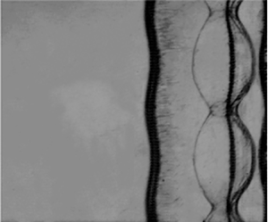
Figure 3. (a) Schlieren images showing an initial flat air/SF $_6$ interface impacted successively by a planar incident shock and a reflected shock. (b) An
  $x$–
$x$– $t$ diagram showing the trajectories of the interface and waves. The unit of numbers in (a) is
  $\mathrm {\mu }$s. The theoretical result in (b) refers to the prediction of inviscid 1-D gas dynamics theory. Abbreviations used are as follows: IS, incident shock; II, initial interface; RS
 $_1$, first reflected shock; SI, shocked interface; TS
 $_1$, first transmitted shock; RTS, reflected transmitted shock; TS
 $_2$, second transmitted shock; RW
 $_1$, first rarefaction wave; RRW
 $_1$, reflected rarefaction wave; CW
 $_1$, compression wave; RCW
 $_1$, reflected compression wave.
We note that, compared with the work of Andronov et al. (Reference Andronov, Bakhrakh, Meshkov, Mokhov and Nikiforov1976), the initial interface in this work is much thinner, and the growth of the interface thickness (particularly after the impact of reshock) is also much slower. This discrepancy can be ascribed mainly to two factors. First, as compared to the membrane technique adopted by Andronov et al. (Reference Andronov, Bakhrakh, Meshkov, Mokhov and Nikiforov1976) (i.e a thin organic film of thickness  $0.3\unicode{x2013} 0.5\ \mathrm {\mu }$m is used to separate two gases), the soap-film technique used in this work can largely eliminate high-wavenumber perturbations and three-dimensionality at the initial interface. Hence the initial interface in this work is flatter with fewer undesired perturbations, and accordingly its thickness grows more slowly than that of Andronov et al. (Reference Andronov, Bakhrakh, Meshkov, Mokhov and Nikiforov1976). Second, the air/SF
 $_6$ interface here is a fast/slow configuration, while the air/He interface in the experiment of Andronov et al. (Reference Andronov, Bakhrakh, Meshkov, Mokhov and Nikiforov1976) is a slow/fast configuration. These two configurations usually present different instability growths. Note that the slow/fast configuration refers to an A/B gas interface for which the sound speed of gas A is less than that of gas B, and the fast/slow configuration refers to an A/B gas interface for which the sound speed of gas A is larger than that of gas B (Samtaney, Ray & Zabusky Reference Samtaney, Ray and Zabusky1998).
Although a gas concentration detector is adopted to measure the oxygen concentration of the gas mixture exhausted from the outflow hole, it can only ensure a high concentration of SF $_6$ on the right side of the interface rather than directly measuring the mass fraction of SF
 $_6$. In this work, we estimate the mass fraction of SF
 $_6$ using the following method. For a planar shock impacting a flat light/heavy interface, the subsequent flow is composed of four uniform regions separated by a reflected shock, a transmitted shock and the interface. According to 1-D gas dynamics theory, we can establish relations for the flow parameters on both sides of the reflected and transmitted shocks. With the compatibility relation at the interface (i.e. velocity and pressure continuity), the following equation can be derived:
 \begin{equation} \left[\frac{(\varLambda_2-1) \rho_1}{(\varLambda_1-1) \rho_2}\right]^{1 / 2} \frac{P_t-1}{(P_t \varLambda_2+1)^{1 / 2}}=\frac{P_i-1}{(P_i \varLambda_1+1)^{1 / 2}}-\left(\frac{\rho_1}{\rho_1^{\prime}}\right)^{1 / 2} \frac{P_t-P_i}{(P_t \varLambda_1+P_i)^{1/2}}, \end{equation}
where
 \begin{equation} \left.\begin{array}{c@{}} \varLambda_1=(\gamma_1+1)/(\gamma_1-1),\\[2pt] \varLambda_2=(\gamma_2+1)/(\gamma_2-1),\\[2pt] P_i=1+2\gamma_1/(\gamma_1+1)(M_i^2-1),\\[2pt] \rho_1/\rho_1^{\prime}=[(\gamma_1-1) M_i^2+2]/[(\gamma_1+1) M_i^2]. \end{array}\right\} \end{equation}
Here,  $\gamma _1$ and
  $\rho _1$ are respectively the specific heat ratio and the fluid density on one side of the interface where the shock wave stays initially, and
  $\gamma _2$ and
  $\rho _2$ are the specific heat ratio and the fluid density on the other side, respectively. Also,
  $P_i$ (
 $P_t$) is the pressure ratio across the incident shock (transmitted shock),
  $\rho _1^{\prime }$ is the fluid density behind the incident shock, and
  $M_i$ is the Mach number of the incident shock. In experiment, the gas on the left side of the interface is pure air. The incident shock has measured speed 445.0 m s
 $^{-1}$ before its collision with the inner interface, corresponding to
  $M_i = 1.29$. The value of the mass fraction is obtained by an iterative method via numerical calculation. Specifically, giving an arbitrary initial value between 0 and 1 for the mass fraction of SF
 $_6$ on the right side of the interface, the flow parameters on the right side (e.g.
  $\rho _2$ and
  $\gamma _2$) can be obtained. Substituting the known parameters into (3.1), the pressure ratio across the transmitted shock (
 $P_t$) can be solved, and then the strength of the transmitted shock is available. If the calculated strength of the transmitted shock is stronger than the measured one, then the value of the mass fraction is reduced; otherwise, it is increased. This process is repeated many times until the calculated value is in good agreement with the measured one (i.e. their difference is lower than 0.1 %). For the unperturbed case here, the mass fraction of SF
 $_6$ is calculated to be 99.5 %. With this value, the flow velocity behind TS
 $_1$ is calculated to be 97.8 m s
 $^{-1}$ based on gas dynamics theory, which agrees reasonably with the experimental measurement (
 $97.7 \pm 0.8\ \textrm {m}\ \textrm {s}^{-1}$). This demonstrates good reliability of the present calculation method. Also, it indicates a negligible influence of soap droplets on the flow.
An  $x$–
$x$– $t$ diagram illustrating the trajectories of the interface and waves is given in figure 3(b), where the prediction of 1-D gas dynamics theory is also given for comparison. Generally, the experimental result is in good agreement with 1-D gas dynamics theory, which indicates a negligible influence of unexpected experimental factors (e.g. the soap film, the thin filaments and the small holes) on the flow field. Note that although the interface becomes a turbulent mixing zone after the impact of RRW
 $_1$, its average position still agrees reasonably with the theoretical prediction. The velocities of IS and TS
 $_1$ are measured to be
  $445.1\pm 1.0\ \textrm {m}\ \textrm{s}^{-1}$ and
 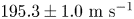 $195.3\pm 1.0\ \textrm {m}\ \textrm {s}^{-1}$, respectively. With these measured values, the volume fraction of SF
 $_6$ on the right side of the interface is calculated to be 99.5 % according to 1-D gas dynamics theory. The Atwood number of the interface, defined as
  $A=(\rho _2-\rho _1)/(\rho _2+\rho _1)$, is 0.71 after the impact of IS. We note that according to the definition of the Atwood number,
  $A$ is negative relative to the propagation of RTS. The interface attains a jump velocity 97.75 m s
 $^{-1}$ immediately after the IS passage and then slows down quickly to
  $-36.21\ \textrm {m}\ \textrm {s}^{-1}$ due to the RTS impact. Afterwards, the interface is impacted successively by the subsequent waves, including RRW
 $_1$ and the reflected compression wave (RCW
 $_1$), and finally tends to be stationary. The present result provides a clear background flow, which is helpful for understanding the reshocked RMI with initial perturbations at either the interface or the reflected shock discussed in the following sections.
Note that in the present experiments, the incident shock is weak, thus the post-shock flow can be assumed to be laminar and incompressible. Hence the thickness of the boundary layer in the post-shock flow ( $\delta ^*$) can be estimated by
 \begin{equation} \delta^*=1.72\sqrt{\frac{\mu x}{\rho\,\Delta v}}. \end{equation}
Here,  $x\approx 30$ mm, which corresponds to the maximum distance travelled by the interface during the experimental time. The viscosity coefficient and density of pure air (SF
 $_6$) under the experimental temperature and pressure are
  $\mu = 1.83 \times 10^{-5}\ \textrm {Pa}\ \textrm {s}$ (
 $= 1.60 \times 10^{-5}\ \textrm {Pa}\ \textrm {s}$) and
  $\rho = 1.204\ \textrm {kg}\ \textrm {m}^{-3}$ (
 $= 6.143\ \textrm {kg}\ \textrm {m}^{-3}$), respectively. The velocity of the post-shock flow is
  $\Delta v= 97.8~\textrm {m}~\textrm {s}^{-1}$. According to (3.3), the maximum thickness of the boundary layer in the post-shock air (SF
 $_6$) flow is calculated to be approximately 0.12 mm (0.05 mm), which is much smaller than the inner height of the test section (6.0 mm). This indicates a negligible influence of the boundary layer on the interface development for the experimental time in this work, which is confirmed by the good agreement between the experiment result and the 1-D gas dynamics theory.
4. Configuration I: RMI at a single-mode interface with a planar reshock
In this section, the RMI at a single-mode interface with a planar reflected shock is examined. Detailed parameters corresponding to the initial conditions for cases 1–3 are listed in table 2. Developments of the interface and wave patterns illustrated by sequences of schlieren images are shown in figure 4. Since the evolution processes for cases 1–3 are similar, here we take case 1 as an example to detail the evolution process. The single-mode initial interface looks quite thick prior to the shock impact ( $-32\ \mathrm {\mu }$s), which is ascribed to the superposition of the filaments on the upper and lower observation windows. After the IS impact, the interface moves downwards and presents a clear and distinct single-mode shape (68
  $\mathrm {\mu }$s), which demonstrates good reliability of the present interface-formation method. Meanwhile, the shocked interface SI develops symmetrically with a gradually increasing amplitude. After reshock, two waves (TS
 $_2$ and RW
 $_1$) are produced. Meanwhile, the interface amplitude reduces quickly to zero (called phase inversion) and then increases continuously with opposite phase (448
  $\mathrm {\mu }$s).

Figure 4. Representative schlieren images illustrating the developments of interface and wave patterns for RMI with a uniform reflected shock. The inserted numbers are in  $\mathrm {\mu }$s. The symbols are the same as those in figure 3.
Dimensionless variations of the interface amplitude with time before reshock for cases 1–3 are plotted in figure 5(a). Time is normalized by  $kv_i(t-t^*)$, where
  $v_i$ is the linear growth rate calculated by the impulsive model (Richtmyer Reference Richtmyer1960), and
  $t^*$ is the end time of the startup phase (Lombardini & Pullin Reference Lombardini and Pullin2009). The amplitude is normalized by
  $k (a-a^*)$, with
  $a^*$ being the amplitude at
  $t^*$. As we can see, the interface amplitude increases linearly for all cases, and also the normalized data for cases 1–3 collapse quite well. For the linear growth of RMI, Richtmyer (Reference Richtmyer1960) has proposed an impulsive model for the linear growth rate under the incompressible, inviscid flow assumption, which is written as
 \begin{equation} \frac{{\rm d}a}{{\rm d}t}=k A^+\,\Delta V_1\,a_0^+,\end{equation}
where  $k=2{\rm \pi} /\lambda$ is the wavenumber,
  $\Delta V_1$ is the jump velocity of the interface caused by the shock impact,
  $A^+$ is the post-shock Atwood number, and
  $a_0^+=a_0(1-\Delta V_1/V_s)$ is the post-shock amplitude, with
  $V_s$ being the incident shock velocity. As shown in figure 5(a), the impulsive model gives a good prediction of the instability growth before reshock for all cases. This gives a further demonstration that the interface development is in the linear regime at the time of reshock.

Figure 5. Dimensionless variations of the interface amplitude with time for cases 1–3, (a) before and(b) after reshock.
In previous experiments of the reshocked RMI (Vetter & Sturtevant Reference Vetter and Sturtevant1995; Leinov et al. Reference Leinov, Malamud, Elbaz, Levin, Ben-Dor, Shvarts and Sadot2009; Mohaghar et al. Reference Mohaghar, Carter, Pathikonda and Ranjan2019), the interface enters a strong nonlinear or turbulent mixing stage at the time of reshock (the linear stage is very short) and thus presents a complex morphology that is difficult to characterize. In addition, the reshock event is essentially the process of a shock wave interacting simultaneously with a density interface and a vortex layer, which is very difficult to model. So far, only two empirical models applicable to specific interface configurations have been developed. One reshock model, applicable to interfaces with initial three-dimensional multi-mode perturbations, was proposed by Mikaelian (Reference Mikaelian1989), who found that the post-reshock growth rate is insensitive to the pre-reshock one. The model is expressed as  ${\textrm {d}h_2}/{\textrm {d}t}= C\,\Delta V_2\,A_r^+$, where
  $h_2$ is the overall width of the mixing zone (i.e. the distance between the spike and bubble tips for the present experiments),
  $\Delta V_2$ is the jump velocity of the interface caused by the reflected shock,
  $A_r^+$ is the post-reshock Atwood number, and
  $C= 0.28$ is an empirical coefficient. Another empirical model applicable to initial two-dimensional single-mode interfaces was proposed by Charakhch'An (Reference Charakhch'An2000), who found that the post-reshock growth rate depends weakly on the pre-reshock amplitude and wavenumber, but strongly on the pre-reshock growth rate. The model is written as
  ${\textrm {d}h_2}/{\textrm {d}t}= \beta \,\Delta V_2\,A_r^+ +{\textrm {d}h_1}/{\textrm {d}t}$, where
  ${\textrm {d}h_1}/{\textrm {d}t}$ is the growth rate of the mixing width just before reshock, and
  $\beta = 1.25$ suggested by Charakhch'An (Reference Charakhch'An2000). The validity of the above models has been verified preliminarily by both experiment (Leinov et al. Reference Leinov, Malamud, Elbaz, Levin, Ben-Dor, Shvarts and Sadot2009) and simulation (Ukai et al. Reference Ukai, Balakrishnan and Menon2011).
Differing from previous experiments, the reshocked RMI considered in this work is a more fundamental case, in which the interface evolution is within the linear regime at the time of reshock. For this case, Mikaelian (Reference Mikaelian1985) has proposed a linear model to predict the growth rate after reshock:
 \begin{equation} \frac{{\rm d}a_2}{{\rm d}t}=k a_r^+\,\Delta V_2\, A_r^++\frac{{\rm d}a_1}{{\rm d}t}, \end{equation}
where the subscripts 1 and 2 denote the quantities before and after reshock, respectively, and  $a_r^+$ is the post-reshock amplitude. Equation (4.2) indicates that if the interface development is in the linear regime at the time of reshock, then the post-reshock growth rate depends heavily on the pre-reshock wavenumber, amplitude and growth rate. Experiments on this reshocked RMI are scarce due to the difficulty in precise control of the initial interface shape. The present results provide a rare opportunity to examine such a reshocked RMI and also to verify the model of Mikaelian (Reference Mikaelian1985).
Dimensionless variations of the interface amplitude with time after reshock for cases 1–3 are plotted in figure 5(b). Time is scaled as  $kv_2(t-t^*_r)$, where
  $v_2$ is the post-reshock growth rate measured from experiment, and
  $t^*_r$ is the time of reshock. The amplitude is scaled as
  $k (a_2-a^*_{r})$, with
  $a^*_{r}$ being the interface amplitude at
  $t^*_r$. Note that in this work, the amplitude of the initial interface is defined as positive and thus the interface amplitude after phase inversion is negative. As we can see, the interface amplitude grows linearly with time after reshock for all cases, and the data for cases 1–3 collapse quite well. The original Mikaelian model underestimates the post-reshock perturbation growth. A major reason is that in the present experiments, the interface is a slow/fast configuration relative to the propagation of the reflected shock, which is different from the fast/slow case considered by Mikaelian (Reference Mikaelian1985). Previous studies have shown that the RMI at a slow/fast interface exhibits noticeable differences from the fast/slow case (Meyer & Blewett Reference Meyer and Blewett1972; Vandenboomgaerde, Mügler & Gauthier Reference Vandenboomgaerde, Mügler and Gauthier1998). Here, we introduce a new post-reshock parameter suggested originally by Vandenboomgaerde et al. (Reference Vandenboomgaerde, Mügler and Gauthier1998) into the Mikaelian model (Mikaelian Reference Mikaelian1985), and the modified model is expressed as
 \begin{equation} \frac{{\rm d}a_2}{{\rm d}t}=k\,\Delta v_2\left( \frac{A_r^+ a_r^++A_r^- a_r^-}{2} \right)+\frac{{\rm d}a_1}{{\rm d}t}, \end{equation}
where the superscripts ‘ $-$’ and ‘
 $+$’ denote the variables before and after the reshock, respectively. Note that (4.3) is essentially an empirical model since it takes an empirical combination of the averages of the pre- and post-shock amplitudes and Atwood number for approximating compressibility effect. For rigorous theories of the RMI, readers are referred to previous works (Richtmyer Reference Richtmyer1960; Wouchuk Reference Wouchuk2001a,Reference Wouchukb; Sohn Reference Sohn2003; Zhang, Deng & Guo Reference Zhang, Deng and Guo2018a). As shown in figure 5(b), (4.3) gives a good prediction of the post-reshock growth for the three cases. It demonstrates that the modelling by Mikaelian (Reference Mikaelian1985) is reasonable for the reshocked RMI in configuration I where the interface is at the linear regime at the time of reshock. The present finding is an important supplement to the knowledge of the reshocked RMI. More importantly, it is a basis for understanding more complex reshocked RMI such as that in configurations II and III.
5. Configuration II: RMI at a flat interface with a sinusoidal reshock
A key issue for the reshocked RMI experiment of configuration II is to create a controllable, repeatable, sinusoidal reflected shock. In this work, the rippled reflected shock is generated by an incident planar shock reflecting off a sinusoidal wall, as sketched in figure 1(b). To verify the method reliability, the dynamics of the sinusoidal reshock generated in experiment is first examined. Typical schlieren images illustrating the generation and propagation of the sinusoidal shock are shown in figure 6(a). An incident planar shock propagates in air at the beginning. Later, it reflects off the sinusoidal wall, and a rippled reflected shock with a sine-like shape is generated immediately. As time proceeds, the sinusoidal shock wave propagates upstream with its amplitude decaying gradually, and finally recovers to a uniform planar shock. Bates (Reference Bates2004) has derived a linear solution for the variation of the amplitude of a sinusoidal shock propagating in inviscid fluids. Comparison between the present experimental result and Bates’ prediction for the variation of the rippled shock amplitude is given in figure 6(b), where time is normalized by  $\tau =V_rkt$, with
  $V_r$ being the average velocity of the rippled shock. As we can see, there is a small discrepancy between the experimental result and the theoretical prediction at the early stage. After
  $\tau > 5.0$, the experimental result agrees well with Bates’ prediction. As far as we know, this is the first experimental confirmation that Bates’ theory is valid for describing a sinusoidal reflected shock.

Figure 6. (a) Schlieren images showing the generation of the rippled reflected shock. (b) Normalized variation of the amplitude of the rippled shock with time. Time is normalized as  $\tau =V_rkt$, with
  $V_r$ being the average speed of the rippled shock. The unit of numbers in (a) is
  $\mathrm {\mu }$s.
The RMI at a flat interface with a sinusoidal reshock belongs to non-standard RMI (i.e. a rippled shock impacting a flat interface) originally proposed by Ishizaki et al. (Reference Ishizaki, Nishihara, Sakagami and Ueshima1996), which has never been realized in an experiment with satisfactory initial conditions. In previous experiments of non-standard RMI, the rippled shock is generated by an incident planar shock passing across one or multiple solid cylinders (Zou et al. Reference Zou, Liu, Liao, Zheng, Zhai and Luo2017, Reference Zou, Al-Marouf, Cheng, Samtaney and Luo2019; Liao et al. Reference Liao, Zhang, Chen, Zou, Liu and Zheng2019). Under this circumstance, unexpected waves and structures such as Mach stems and triple points are produced behind the rippled shock, which greatly contaminate the propagation of the ripple shock and further influence the instability growth. The sinusoidal shock generated in this work provides a rare opportunity to examine the non-standard RMI with ideal initial conditions. For this purpose, the initial interface is set to be flat for case 4, and the corresponding initial parameters are listed in table 2.
Experimental schlieren images together with numerical schlieren images and pressure contour images for case 4 are given in figure 7. After an incident planar shock passes across a flat air/SF $_6$ interface, the interface moves downwards. As the TS
 $_1$ reflects off the sinusoidal wall, a rippled reflected shock is generated immediately, which later interacts with the flat interface, giving rise to a non-standard RMI. As expected, before the RTS impact, the interface keeps flat and thin with no instability (239
  $\mathrm {\mu }$s). The pressure contour images show the existence of a non-uniform pressure field behind the rippled shock (239
  $\mathrm {\mu }$s), which indicates that the strength of the rippled shock is non-uniform along the shock front. An interface impacted by such a rippled shock would attain a non-uniform jump velocity, giving rise to the variation of interface amplitude. This mechanism was first called velocity perturbation by Ishizaki et al. (Reference Ishizaki, Nishihara, Sakagami and Ueshima1996).

Figure 7. Comparisons between the experimental schlieren (top) and numerical schlieren (middle) images, and pressure contour images (bottom) from simulation, for case 4. The numbers inserted are in  $\mathrm {\mu }$s. The symbols are the same as those in figure 3.
Time-varying amplitude of the interface after the impact of reshock is plotted in figure 8. Since the interface is first impacted by the trough and then by the crest of the rippled shock, it presents a visible small perturbation after the passage of the rippled shock (20  $\mathrm {\mu }$s). Afterwards, this small perturbation increases almost linearly with time (
 $t< 80\ \mathrm {\mu }$s) with an opposite phase. The growth rate obtained by a linear fit of experimental data is listed in table 3. It is found that the post-reshock growth rate for case 4 is comparable to the rates for cases 1–3. This differs greatly from the incident shock situation, where the growth of a flat interface induced by a rippled incident shock is much slower than that of a perturbed interface induced by a planar incident shock (Zhang et al. Reference Zhang, Wu, Zou, Zheng, Li, Luo and Ding2018b; Zou et al. Reference Zou, Al-Marouf, Cheng, Samtaney and Luo2019).

Figure 8. Variation of the interface amplitude after the impact of reshock for case 4.
Table 3. The perturbation growth rates induced by velocity perturbation ( $v_{imp}$) and baroclinic vorticity (
 $v_\tau$), as well as the total post-reshock growth rate (
 $v_2$) predicted by (6.1). Here,
  $v_1$ denotes the pre-reshock growth rate calculated by the impulsive model.

Ishizaki et al. (Reference Ishizaki, Nishihara, Sakagami and Ueshima1996) has studied numerically the instability at a uniform slow/fast interface impacted by a sinusoidally rippled shock, and found that in addition to a pressure perturbation mechanism existing in the standard RMI, velocity perturbation is another driving factor for the growth of the non-standard RMI. Taking pressure perturbation and velocity perturbation into account, Ishizaki et al. (Reference Ishizaki, Nishihara, Sakagami and Ueshima1996) proposed a model for the growth rate of the non-standard RMI, which is written as
 \begin{equation} v = \frac{U_I}{ V_S}\,\dot{ a_s} (t_0) - \frac{\Delta g}{ \omega} \cos \phi ,\end{equation}
where  $\dot { a_s} (t_0)$ is the growth rate of the amplitude of the rippled shock when it encounters the interface. The first term on the right-hand side of (5.1) corresponds to the growth rate caused by velocity perturbation. The second term corresponds to the growth rate caused by pressure perturbation, where
  $\Delta g$ and
  $\omega$ are the amplitude and frequency of the oscillating pressure, respectively, and
  $\phi$ is the phase of the oscillating shock at
  $t_0$. Assuming that the second term is proportional to the first term, a parameter
  $D$ was introduced by Ishizaki et al. (Reference Ishizaki, Nishihara, Sakagami and Ueshima1996) to simplify the formula to
 \begin{equation} v_a = D\,\frac{U_I}{ V_S}\,\dot{ a_s} (t_0) , \end{equation}
where  $D$ is an empirical constant;
  $D= 0.66$ is suggested by Ishizaki et al. (Reference Ishizaki, Nishihara, Sakagami and Ueshima1996).
The linear growth rate obtained here enables us to examine the theory of Ishizaki et al. (Reference Ishizaki, Nishihara, Sakagami and Ueshima1996). As shown in figure 8, the Ishizaki model underestimates the present experimental and numerical results. A possible reason is that the value of the coefficient  $D$ in the Ishizaki model is not constant but depends on the initial conditions such as the shock Mach number. Despite the deviation, the present result indicates that velocity perturbation is important and should be considered for the RMI with a rippled reshock. The finding here suggests deriving a more accurate model by considering separately the velocity perturbation and pressure perturbation, which will be addressed in § 6.
6. Configuration III: RMI at a single-mode interface with a sinusoidal reshock
In this section, we will examine the most complex case: the RMI at a single-mode interface with a sinusoidal reshock. Beside experiment, numerical simulation is also performed to gain more flow details, which are necessary for an in-depth flow analysis. Detailed parameters corresponding to the initial conditions for cases 5 and 6 are listed in table 2. The only difference in initial setting among cases 3, 5 and 6 is the shape of the reflected shock. Specifically, for case 3, the reflected shock is uniform, while for case 5 (case 6), the reflected shock possesses a sinusoidal perturbation that is in phase (out of phase) with the distorted interface. This setting allows us to examine the influence of the reflected shock on the instability growth. Comparisons between the schlieren images from experiment, the schlieren images from numerical simulation and the pressure contour images from numerical simulation for cases 3, 5 and 6 are given in figure 9. Generally, numerical simulations reproduce well the experimental results for both the interface deformation and the wave propagation for all three cases. This enhances our confidence in the accuracy of the numerical flow field obtained, which can greatly facilitate the mechanism analysis. It is found that the instability growth after reshock is quicker than that of a uniform reflected shock for case 5 where the rippled shock has an in-phase perturbation relative to the perturbed interface, and slower for case 6 where the rippled shock has an anti-phase perturbation relative to the interface. It means that the rippled shock with an in-phase perturbation relative to the perturbed interface can promote the instability growth, whereas the rippled shock with an anti-phase perturbation will suppress the instability growth. A qualitative interpretation for this phenomenon is given below. As indicated by the pressure contour snapshots for cases 5 and 6, the rippled shock is non-uniform along the shock front, thus velocity perturbation is evident, as has been found in reshocked RMI configuration II. Another important mechanism driving the instability growth is pressure perturbation, which is a common mechanism in the standard RMI. Since the perturbation phase of TS $_2$ (RW
 $_1$) remains invariant for cases 3, 5 and 6, the perturbation growth induced by pressure perturbation has an identical direction for the three cases. If the instability growth caused by velocity perturbation, which is a unique mechanism in the rippled-shock-induced RMI, has the same direction as that of pressure perturbation, then the instability growth would be promoted. While the instability growth caused by velocity perturbation has direction opposite to that of pressure perturbation, the instability growth would be inhibited. In the present experiments, the initial phase of the rippled shock determines the shock strength distribution, and further determines the direction of velocity perturbation. The present analysis reasonably explains the quicker (slower) instability growth in case 5 (case 6) than that in case 3. In particular, for case 6 with an anti-phase rippled shock, the inhibition effect is so strong that the interface does not invert during the duration of the experiment.

Figure 9. Comparisons between the experimental schlieren (top) and numerical schlieren (middle) images, and pressure contour images (bottom) from simulation, for cases 3, 5 and 6. The numbers inserted are in  $\mathrm {\mu }$s. The symbols are the same as those in figure 3.
Variations of the amplitude of the rippled shock with time for cases 5 and 6 from experiment and simulation are plotted in figure 10. The last data point for each case corresponds to the amplitude of the rippled shock at the time of reshock. The initial amplitudes of the rippled shock for the two cases are different, and neither value is consistent with the prediction of 1-D shock dynamics theory. Moreover, the shock amplitude for case 6 decays more quickly than that of case 5, and both cases deviate from Bates’ prediction. A major reason for these discrepancies is that although the transmitted shock TS $_1$ has recovered visually to a uniform planar shock before it encounters the sinusoidal wall, the pressure field behind TS
 $_1$ is still non-uniform, i.e. the flow in front of the rippled reflected shock is non-uniform, rather than a uniform or stationary pressure field assumed by Bates (Reference Bates2004). As the rippled reshock propagates upstream in such a non-uniform pressure field, the post-reshock pressure distribution should differ greatly from the ideal situation considered by Ishizaki et al. (Reference Ishizaki, Nishihara, Sakagami and Ueshima1996) and Bates (Reference Bates2004). As can be seen from the pressure contours in figure 9, the pressure difference between the high and low pressure regions behind the rippled shock for case 6 is much larger than that of case 5. This reasonably explains the quicker decay of shock amplitude in case 6 than in case 5. It should be emphasized that the decay rate of the rippled shock amplitude is closely related to the magnitude of velocity perturbation, which will be analysed hereinafter.

Figure 10. Variations of the rippled shock amplitude with time from experiment and simulation for cases 5 and 6. The last data point for each case corresponds to the shock amplitude just as it encounters the interface.
Temporal variations of the interface amplitude from experiment and simulation for cases 3, 5 and 6 are plotted in figure 11. As expected, before the RTS impact, the growths of the interface amplitude for the three cases collapse quite well. At the very beginning, there is a startup phase, at which the perturbation growth rate increases gradually from zero to a certain value. Then the perturbation amplitude increases linearly at a constant growth rate. After the RTS impact, the instability growths for the three cases exhibit considerable differences. For cases 3 and 5, the interface amplitude reduces quickly to zero, and then increases with the opposite phase. For case 6, the interface amplitude first reduces to a smaller value, then keeps nearly invariant for a period of time (i.e. phase inversion cannot be completed in a short time), and later begins to increase with an opposite phase. The present result shows a strong dependence of the phase of the rippled shock on the instability growth. It is seen that the modified Mikaelian model is invalid for cases 5 and 6 with a rippled reshock, even though it provides an accurate prediction for cases 1–3 with a planar reshock. A major reason is that for RMI with a rippled reflected shock, which belongs to non-standard RMI, pressure perturbation and velocity perturbation collectively drive the instability growth, but the latter was not considered in the model of Mikaelian (Reference Mikaelian1985).

Figure 11. Temporal variations of the interface amplitude for cases 3, 5 and 6 from experiment, simulation and theoretical prediction.
The analyses on the reshocked RMI in configurations II and III in §§ 4 and 5 tell us that the growth of RMI with a rippled reflected shock could be dominated by three factors: velocity perturbation, pressure perturbation and pre-reshock growth rate. This guides us to model the growth of the reshocked RMI in configuration II. Assuming that the instability growth is in the linear regime (which is consistent with the present experiments), the post-reshock growth rate can be obtained via a superposition of these three parts:
 \begin{equation} v_2=v_\tau+v_{imp}+v_1, \end{equation}
where  $v_\tau$ is the growth rate induced by pressure perturbation,
  $v_{imp}$ is the growth rate caused by velocity perturbation, and
  $v_1$ is the pre-reshock growth rate, which can be calculated by the impulsive model.
Direct estimation of pressure perturbation on the instability growth is quite difficult. As an alternative method, Samtaney & Zabusky (Reference Samtaney and Zabusky1994) proposed to calculate baroclinic vorticity deposited on the interface during the shock–interface interaction, and the interface development caused by pressure perturbation can be regarded equivalently as the evolution of a vortex sheet distributed along the interface. Following this strategy, Li et al. (Reference Li, Ding, Luo and Zou2022a) proposed a vortex model for non-standard RMI in the convergent geometry, and the model validity was verified by experiment. In this work, we will estimate the growth rate caused by pressure perturbation using a similar method. Setting a Cartesian coordinate system at the moving interface, the sinusoidal interface and the rippled reflected shock can be described approximately as
 \begin{equation} \left.\begin{array}{c@{}} y(x)=a\cos(kx),\\[2pt] y_s(x)=\bar{y}_s+a_s\cos(kx),\\ \end{array}\right\} \end{equation}
where  $\bar {y}_s$ is the average position of the rippled shock. Thus the velocity of the rippled shock is
 \begin{equation} V_s(x)=V_s+\dot{a}_s\cos(kx). \end{equation}
Equation (6.3) indicates that the strength of the ripple shock varies continuously along the shock front. In particular, the rippled shock is the strongest at its crest and the weakest at its trough, where the crest (trough) is defined as the shock tip that has a maximum (minimum) value of  $y$. As the rippled shock interacts with a perturbed interface, it affects the interface evolution in two ways. On the one hand, the interface accelerated by such a rippled shock attains a non-uniform jump velocity (i.e. velocity perturbation), giving rise to an instability growth immediately. On the other hand, baroclinic vorticity is deposited at the interface due to the misalignment of pressure and density gradients, which later drives the interface evolution.
Differing from the model of Ishizaki et al. (Reference Ishizaki, Nishihara, Sakagami and Ueshima1996), in this work, the growth rate caused by velocity perturbation is estimated by
 \begin{equation} v_{imp}=\frac{(V_{max}-V_{min})}{2}, \end{equation}
where  $V_{max}$ refers to the maximum velocity of the interface at the position where the rippled shock wave is the strongest, and
  $V_{min}$ refers to the minimal velocity of the interface at the position where the rippled shock wave is the weakest. With the measured growth rate of the rippled shock amplitude, the shock strength distribution can be obtained according to (6.3). Then
  $V_{max}$ and
  $V_{min}$ can be calculated readily according to 1-D gas dynamics theory.
Next, we calculate the growth rate caused by baroclinic vorticity. For a slow/fast inclined interface impacted by a planar shock wave, Samtaney & Zabusky (Reference Samtaney and Zabusky1994) have derived an analytical solution for the baroclinic vorticity deposited per unit length of the interface:
 \begin{equation} \frac{{\rm d}\varGamma}{{\rm d}s}=\frac{4c_0}{\gamma+1}\left(1-\frac{1}{\sqrt{\eta}}\right) \frac{M^2-1}{1+\dfrac{2\gamma}{\gamma+1}\,(M^2-1)}\sin\alpha, \end{equation}
where  $M$ is the shock Mach number,
  $\eta$ is the density ratio across the interface,
  $c_0$ is the sound speed, and
  $\alpha$ is the angle between the shock and the interface. Based on the geometric relationship, we have
 \begin{equation} \sin\alpha=k(a-a_s)\,\frac{{\rm d}\kern0.06em x}{{\rm d}s}\sin (kx). \end{equation}
Incorporating equation (6.6) into (6.5), we have
 \begin{equation} \frac{{\rm d}\varGamma}{{\rm d}\kern0.06em x}=\frac{4c_0}{\gamma+1}\left(1-\frac{1}{\sqrt{\eta}}\right) \frac{M(x)^2-1}{1+\dfrac{2\gamma}{\gamma+1}\,(M(x)^2-1)}\,k(a-a_s)\sin (kx). \end{equation}
Approximating the interface as a straight line, with (6.7), the horizontal velocity at an arbitrary position of the interface induced by the vortex sheet can be estimated based on the Birkhoff–Rott equation:
 \begin{equation} v_\tau(x)=\int_{x-c_0^+t}^{x+c_0^+t}{\frac{1}{2{\rm \pi}\,|x-x'|}}\,{\frac{{\rm d}\varGamma}{{\rm d}\kern0.06em x}}(x')\,{\rm d}\kern0.06em x', \end{equation}
where  $c_0^+$ is the sound speed behind the transmitted shock TS
 $_2$. With (6.8), the growth rate caused by baroclinic vorticity can be obtained readily. Incorporating (6.4), (6.8) and the pre-reshock growth rate calculated by the impulsive model into (6.1), a linear model for RMI at a single-mode interface with a rippled reflected shock is obtained.
The calculated growth rates caused by velocity perturbation and baroclinic vorticity, as well as the total growth rate after the impact of reshock, for cases 3–5 are listed in table 3. The quantitative data indicate that the instability growth caused by velocity perturbation has an identical direction to that of baroclinic vorticity for case 5, and an opposite direction to that of baroclinic vorticity for case 6. This gives strong evidence for our qualitative analysis based on pressure contour images. As shown in figure 11, the present model gives a good prediction of the post-reshock instability growth for both in-phase and anti-phase cases. Moreover, it gives a reasonable prediction of the post-reshock growth for the reshocked RMI in configuration II, as shown in figure 8. This reveals the generality of the present theory. It should be pointed out that a point vortex can impart a velocity to its surrounding fluid only after its information arrives there (propagates at the sound speed). Hence at the very beginning, the predicted growth rate increases gradually from zero to a certain value (figure 11), corresponding to the startup process of RMI known from the pressure perturbation perspective (Richtmyer Reference Richtmyer1960; Lombardini & Pullin Reference Lombardini and Pullin2009). The present model provides fundamental guidance for modulating the instability growth in confined spaces.
7. Conclusions
In this work, a novel technique to create a controllable, repeatable, sinusoidal reflected shock is developed. Specifically, the rippled reflected shock is generated by reflecting an incident planar shock off a precisely manufactured sinusoidal wall. The dynamics of the rippled shock generated in experiment is examined first. It is found that the shock amplitude decays gradually with an evident oscillation, which agrees reasonably with the prediction of Bates (Reference Bates2004). An advanced soap-film technique is adopted to generate discontinuous gas interfaces that are free of three-dimensionality, short-wavelength perturbations and diffusion layer. The 1-D background flow corresponding to a flat air/SF $_6$ interface impacted successively by an incident planar shock and a reflected planar shock is examined first. The trajectories of the interface and waves agree well with the prediction of 1-D gas dynamics theory. These results demonstrate the good reliability of the present experimental methods.
Then the reshocked RMI in three different configurations is studied both experimentally and numerically: RMI at a single-mode interface with a planar reflected shock (configuration I); RMI at a flat interface with a sinusoidal reflected shock (configuration II); RMI at a single-mode interface with a sinusoidal reflected shock (configuration III). For all three configurations, the initial conditions of the experiment are set especially such that the interface evolution is in its linear stage when the reshock arrives. It is found that the amplitude of the reshocked interface increases linearly with time for all three configurations. For configuration I, the growth rate after reshock depends heavily on the pre-reshock amplitude and growth rate, which gives a strong demonstration of the reasonability of the model of Mikaelian (Reference Mikaelian1985). A new parameter for the slow/fast configuration suggested by Vandenboomgaerde et al. (Reference Vandenboomgaerde, Mügler and Gauthier1998) is adopted in the Mikaelian model, and the modified model gives better agreement with the experimental results. Compared with previous experiments on a rippled shock impacting a flat interface, the present experiment on the reshocked RMI in configuration II involves more ideal initial conditions, such as the sinusoidal shock and the flat interface. Results suggest that velocity perturbation plays an important role and should be considered for RMI with a rippled reshock. It is found that the model of Ishizaki et al. (Reference Ishizaki, Nishihara, Sakagami and Ueshima1996) underestimates the present experimental result due to the use of an empirical coefficient.
For configuration III, the instability growth after reshock is different from that of configuration I. Specifically, if the sinusoidal shock is in phase with the interface, then the instability growth after reshock will be promoted, causing a quicker instability growth. If the sinusoidal shock is out of phase with the interface, then the instability growth after reshock will be inhibited, causing a slower instability growth. The reason is that for the in-phase case, velocity perturbation causes an instability growth that has the same direction with pressure perturbation, whereas for the anti-phase case, velocity perturbation causes an instability growth that has an opposite direction to pressure perturbation. It is also found that the non-uniform pressure field in front of the rippled shock greatly affects the post-shock pressure distribution. Specifically, the pressure difference between the high and low pressure regions behind the anti-phase shock is much larger than that in the in-phase case, resulting in different decay rates of the rippled shock for the two cases. As a consequence, the degree of instability inhibition in the anti-phase case is greater than the degree of promotion in the in-phase case. A linear theory, that takes velocity perturbation, baroclinic vorticity and pre-reshock growth rate into account, is developed, which gives a reasonable prediction of the growth of the reshocked RMI in configurations II and III.
Funding
This work was supported by the National Natural Science Foundation of China (12072341, 12122213 and 91952205) and the National Key Research and Development Program of China (2022YFF0504500). The simulations were supported by the Supercomputing Center of University of Science and Technology of China (USTC).
Declaration of interests
The authors report no conflict of interest.


