2.1. Implementation of inlet and outlet conditions

The main challenge of extending the acceleration-driven Poiseuille flow to the pressure-driven Poiseuille flow is to impose the constant pressure inlet and outlet boundary conditions at the particle level which is non-trivial. Following Zheng et al. (Reference Zheng, Garcia and Alder2002), we add a layer of ghost cells on either side of the simulation domain along the $x$-direction to act as infinite reservoirs as shown schematically in figure 2. After the streaming stage in every time step the particles in these ghost cells are deleted and the required number of particles $N_{{req}}$, calculated from $\rho _{\pm }$ (see figure 2), are generated uniformly in the ghost cells and their velocities are sampled from a Gaussian with mean equal to the average velocities in their adjacent cells in the $x$-directions and a standard distribution of $\sqrt {{k_BT_{\pm }}/m}$. This ensures that the inlet and outlet of the system are maintained at the specified states. The calculation of the mean pressure $p_0=p_{{av}}$, the mean density $\rho _0=\rho _{{av}}$ and other inlet and outlet quantities are done using the relations listed in figure 2. For example, the derivative conditions on the velocity $\partial v_{\pm }/{\partial x}$ correspond to the DSMC conditions of $v_{+} \to v_{+1}\equiv v_{in}$ and $v_{-} \to v_{-1}\equiv v_{out}$ at the inlet and outlet, respectively.

The implementation of inlet and outlet conditions also produces noisier data compared with its acceleration-driven counterpart. To resolve this issue, we follow a two-step algorithm. First, we run the code with $N = O(10^5)$ number of computational particles for a shorter period of time with the average velocities in the adjacent cells taken to be a running average of the past 50 time steps. This is done to obtain the steady state inlet and outlet velocities since the velocity is a first-order moment and converges faster even with a fewer number of particles $N = O(10^5)$. The code is then run again with larger $N = O(10^6)$ with the inlet and outlet velocities, which are used as the mean for the Gaussian from which the generated particles are sampled, being taken from the previous run (step 1). The results of this two-step procedure are shown in figure 3, which confirms smoother profiles of hydrodynamic fields (especially the higher-order quantities, such as the tangential heat flux $q_x$ and temperature $T$) than those presented by Zheng et al. (Reference Zheng, Garcia and Alder2002). It may be noted that the particle–wall collisions are modelled as those of fully ‘diffuse’ thermal-wall (Bird Reference Bird1994; Mansour et al. Reference Mansour, Baras and Garcia1997; Pöschel & Schwager Reference Pöschel and Schwager2005; Gupta & Alam Reference Gupta and Alam2017) boundary conditions for both pressure-driven and acceleration-driven flows, see Appendix A for details.

Figure 3. Transverse profiles of the dimensionless (a) streamwise velocity $u_x(x=0,y)$, (b) temperature $T(x=0,y)$ and (c) tangential heat flux $q_x(x=0,y)$ at the midchannel ($x=0$), with parameter values of ${Kn}\,{=}\,0.1$, $\delta p/ p_0=1$ and $AR=L_x/L_y = 3$; see the last paragraph in § 2.3 for the reference scales for dimensionless fields. The red-circled lines denote the data of Zheng et al. (Reference Zheng, Garcia and Alder2002) for the same pressure-driven Poiseuille flow.

Since the hydrodynamic fields in the pressure-driven case vary in both the longitudinal (streamwise) and transverse (cross-stream) directions, we need to have collision cells and averaging cells in two directions, leading to increased computing time. To tackle this issue the code is parallelized by dividing the domain into a number of subdomains, which is equal to the number of processing cores the code is intended to run on. The streaming (including the implementation of the boundary conditions) and collision of particles in different subdomains is carried out simultaneously, and the information of the particles that leave or enter the subdomain is communicated amongst the cores using a message passing interface. The parallelized version of this code is used to run the simulations on the ParamYukti supercomputing cluster at the Jawaharlal Nehru Centre for Advanced Scientific Research (JNCASR).

2.2. Hydrodynamic and flux fields, and the averaging procedure

Referring to figure 2, the flow domain ($L_x\times L_y\times L_z$) is divided into a number of cells, each of size $\delta _x\times \delta _y\times \delta _z$, where $\delta _x$, $\delta _y$ and $\delta _z$ are the dimensions of the cell along the $x$-, $y$- and $z$-directions, respectively; note that the ‘collision’ cells and the ‘averaging’ cells are taken to be identical. The macroscopic average of a particle level quantity $\psi (v)$ in a given cell is defined as

(2.1)\begin{equation} \left\langle \psi(\boldsymbol{v}) \right\rangle_{x,y,z} = \frac{1}{N_t}\sum_t^{N_t} \frac{1}{V_{c}}\sum_{i \in {cell}} \psi ({\boldsymbol v}_i(t)), \end{equation}

where $V_c = \delta _x \delta _y \delta _z$ is the volume of the cell and $N_t$ is the number of snapshots over which the quantity is averaged. Since the pressure-driven Poiseuille flow is invariant along the periodic $z$-direction, we obtain two-dimensional fields of the macroscopic quantities by considering a single cell ($\delta _z = L_z$) in the $z$-direction. The density, velocity and temperature are defined via (Mansour et al. Reference Mansour, Baras and Garcia1997; Uribe & Garcia Reference Uribe and Garcia1999)

(2.2)$$\begin{gather} \rho (x,y) = \left\langle m \right\rangle_{x,y}, \end{gather}$$

(2.3)$$\begin{gather}{\boldsymbol u} (x,y) = \frac{1}{\rho (x,y)}\left\langle m{\boldsymbol v} \right\rangle_{x,y}, \end{gather}$$

(2.4)$$\begin{gather}T (x,y) = \frac{m}{3k_B\rho(x,y)}\left\langle ({\boldsymbol v} - {\boldsymbol u})^2 \right\rangle_{x,y}, \end{gather}$$

which are obtained by setting $\psi (v)=(m, m{\boldsymbol v}, m ({\boldsymbol v}-{\boldsymbol u})^2/3k_B)$ in (2.1). The stress tensor and heat flux vector are accordingly obtained from

(2.5)$$\begin{gather} {\boldsymbol P} (x,y) = \left\langle m({\boldsymbol v}-{\boldsymbol u})({\boldsymbol v}- {\boldsymbol u}) \right\rangle_{x,y}, \end{gather}$$

(2.6)$$\begin{gather}{\boldsymbol q} (x,y) = \tfrac{1}{2}\left\langle m({\boldsymbol v}- {\boldsymbol u})^2(\boldsymbol{v}-\boldsymbol{u}) \right\rangle_{x,y}. \end{gather}$$

Note that the trace of the stress tensor divided by the number of dimensions, $p = (P_{xx} + P_{yy} + P_{zz})/3$, yields the expression for pressure.

The averaging of the hydrodynamic and flux fields, as defined in (2.1), is carried out over multiple snapshots of the system once the system has reached a steady state. The steady state is determined by checking the constancy of the average kinetic energy per particle ($E/N =\sum _i m v_i^2/2N$) in the system, see figure 4(a). Another issue is the maintenance of the inlet ($p_{+}$) and outlet ($p_{-}$) values of the pressure which can be verified from figure 4(b) that displays the streamwise variation of the pressure, $p(x,0)$, at the middle of the channel ($y=0$) – it is clear that $p_{+}/p_0\approx 1.5$ and $p_{-}/p_0\approx 0.5$ as imposed in simulations (viz. figure 2). In addition to validating the present code to correctly reproduce the previous simulation results (Zheng et al. Reference Zheng, Garcia and Alder2002) on the pressure-driven Poiseuille flow in figure 3, the same DSMC code was further validated to simulate acceleration-driven Poiseuille flow and the planar Couette flow of rarefied gases.

Figure 4. (a) Average kinetic energy per particle, $E/N=\sum _i mv_i^2/N$, versus time and (b) the axial variation of the pressure $p(x,0)$ at midchannel $y=0$. Parameter values are as in figure 3.

2.3. Control parameters and reference scales

The main control parameter is the ‘global’ Knudsen number,

(2.7)\begin{equation} {Kn} = \frac{l_f}{L_y} = \frac{1}{\sqrt{2}{\rm \pi} d^2 n_0 L_y}, \end{equation}

which is varied in the range of $0.01 \leq {Kn} \leq 100$ by changing the mean free path $l_f=1/(\sqrt {2}{\rm \pi} n_0 d^2)$ via changing the reference density $\rho _0=m n_0=\rho _{{av}}$ while keeping the channel width $L_y$ constant. The inlet and outlet pressures $p_+$ and $p_-$ are set as

(2.8a,b)\begin{equation} p_+ = p_0 + \frac{\delta p}{2} \quad \text{and} \quad p_- = p_0 - \frac{\delta p}{2}, \end{equation}

such that

(2.9a,b)\begin{equation} p_+ - p_- = \delta p \quad \text{and} \quad \tfrac{1}{2}\left(p_{+} + p_{-}\right) = p_0 \end{equation}

refer to the pressure difference and the mean pressure, respectively, see figure 2.

For most of the presented results, the pressure difference is set to $\delta p = p_0$, which has been chosen such that the forcing terms in (i) the acceleration-driven case $\rho _0 a$ and (ii) the pressure-driven case ${\rm d}p/{{\rm d}{\kern0.7pt}x} \approx \delta p/L_x$ are of the same magnitude for a meaningful comparison between the results of the two sets of studies. We have verified that $1.3 \times 10 ^{-6} \geq \rho _0 a \geq 1.3\times 10^{-10}$ and $1.08 \times 10^{-6} \geq {\rm d}p/{{\rm d}{\kern0.7pt}x} \geq 1.08 \times 10^{-10}$ for the range of Knudsen numbers $0.01 \leq {Kn} \leq 100$, and the forcing terms for four values of ${Kn}$ are shown in table 1. The dimensionless acceleration (Tij & Santos Reference Tij and Santos1994; Mansour et al. Reference Mansour, Baras and Garcia1997; Aoki et al. Reference Aoki, Takata and Nakanishi2002; Gupta & Alam Reference Gupta and Alam2017; Alam et al. Reference Alam, Gupta and Ravichandir2021) is defined as

(2.10)\begin{equation} \hat{a} = \frac{a L_y}{2k_B T_w/m}, \end{equation}

which is a measure of the strength of the flow and represents the body force acting on a gas molecule travelling a distance $L_y$; the numerical value of $\hat {a} = 0.1$ has been chosen for a comparison with the pressure-driven case with $\delta p/p_0=1$. Note that the acceleration-driven flow belongs to the linearized and nonlinear regimes for $\hat {a}\ll 1$ and $O(1)$, respectively. We refer to Appendix B for related details on the local values of the Knudsen number (${{Kn}}(x,y)$), Mach number (${{Ma}}(x,y)$) and Reynolds number (${\textit {Re}}(x,y)$) for both forcings.

Table 1. Comparison of the forcing terms ($\rho _0 a$ and ${\rm d}p/{{\rm d}{\kern0.7pt}x}$) for various Knudsen number (${Kn}$) corresponding to (i) a pressure-difference of $\delta p = p_0$ (and the pressure-gradient is ${\rm d}p/{{\rm d}{\kern0.7pt}x}=\delta p/L_x$) in the pressure-driven Poiseuille flow and (ii) a dimensionless acceleration (2.10) of $\hat {a} = 0.1$ in the acceleration-driven Poiseuille flow. The width and length of the channel are $L_y/d=1860$ and $L_x/d=5580$, respectively, with aspect ratio $AR=L_x/L_y=3$.

The mass and the diameter of the atoms/particles are taken to be unity ($m=d=1$), the Boltzmann constant is taken as $k_B = 0.5$ and the wall temperature is $T_w = T_0 = 1$. The width of the channel is fixed as $L_y = 1860 d$ in most simulations; to study the effect of the channel aspect ratio ($AR=L_x/L_y$), the length of the channel ($L_x$) is increased keeping its width constant such that $3 \leq AR \leq 27$. The effect of pressure gradient is studied by changing the pressure difference ($0.1\leq \delta p/p_0 \leq 1$) by a factor of $10$. All results are presented in dimensionless form: the density is normalized by $\rho _0=\rho _{{av}}$, the temperature by $T_0=T_w$, the velocity by $u_0 = \sqrt {2k_BT_0/m}$, the pressure and stresses by $p_0=(p_{+}+p_{-})/2=p_{{av}}$ and the heat fluxes by $\rho _0 u_0^3/2$. The lengths are rescaled by the channel width $L_y$ such that the streamwise and wall-normal ranges are given by $-AR/2\leq x/L_y \leq AR/2$ and $-0.5 \leq y/L_y \leq 0.5$, respectively.

3.1. Velocity field and the mass flow rate

The contour plots of the streamwise velocity $u_x(x,y)$ and the local mass flux $\rho (x,y)u_x(x,y)$ are displayed in figures 5(a) and 5(b), respectively, at a Knudsen number of ${Kn}=0.05$. It is seen that while the streamwise velocity $u_x$ (figure 5a) increases along the length of the channel (and hence the flow is developing and steady), the local mass-flux $\rho u_x$ (figure 5b,d) also varies slightly along the length of the channel. The effect of rarefaction (${Kn}$) on the transverse and axial profiles of the local mass flux $\rho (x,y)u_x(x,y)$ at $x=0$ and $y=0$, respectively, can be understood from figures 5(c) and 5(d). It is seen that the local mass flux decreases with increasing ${Kn}$ but seems to saturate beyond a critical value of ${Kn}$; the latter can be appreciated from the curves representing ${Kn}=5$ (blue dot–dashed line) and $50$ (magenta dotted line) that are almost indistinguishable from each other.

Figure 5. (a,b) Contour plots of (a) streamwise velocity $u_x(x,y)$ and (b) local mass flux $\rho (x,y) u_x(x,y)$ at ${Kn}=0.05$. (c,d) Variations of (c) $\rho (0,y)u_x(0,y)$ at $x=0$ and (d) $\rho (x,0)u_x(x,0)$ at $y=0$ for different values of ${Kn}$. Parameter values are as in figure 3.

That the pressure-driven Poiseuille flow of a gas is not fully developed (viz. figure 5a; see also the discussion in § 3.3.1) and the local mass flux $\rho (x,y)u_x(x,y)$ (viz. figure 5d) varies axially suggest that the wall-normal velocity $u_y(x,y)$ must be finite as dictated by the continuity equation

(3.1)\begin{equation} \frac{\partial \rho u_x}{\partial x} + \frac{\partial \rho u_y}{\partial y} = 0 . \end{equation}

This is confirmed in figures 6(a) and 6(b), which display the contour plots of $u_y(x,y)$ and $\rho (x,y)u_y(x,y)$, respectively. Ignoring entrance and exit effects, we observe that both the streamwise and wall-normal velocities vary monotonically along the length of the channel. The effect of ${Kn}$ on the transverse profiles of the wall-normal velocity $u_y(0,y)$ at the midchannel ($x=0$) is shown in figure 6(c). The wall-normal velocity profiles closely resemble sine waves, irrespective of the value of ${Kn}$; its amplitude ($\delta u_y=u_y^{max} - u_y(0)$), which is an order smaller compared with the magnitudes of $u_x$, decreases with increase in ${Kn}$, see figure 6(d), and appears to saturate to a constant value at large enough ${Kn}\gg 1$.

Figure 6. (a,b) Contour plots of (a) the wall-normal velocity $u_y(x,y)$ and (b) $\rho (x,y) u_y(x,y)$ for ${Kn}=0.05$. (c,d) Cross-stream variations of the wall-normal velocity $u_y(0,y)$ and (d) $\delta u_y= \max |u_y(0,y)|$ with ${Kn}$. Other parameter values as in figure 5.

From the contour plots of $\rho u_x$ such as in figure 5(b), the mass flow rate of the gas is calculated using

(3.2)\begin{equation} \mathcal{M}({{Kn}}) = \frac{1}{\rho_0 u_0}\int_{{-}0.5}^{0.5} \rho(x,y) u_x(x,y) \,{{\rm d} y}, \end{equation}

where $\rho _0$ is the average density and $u_0 = \sqrt {{2k_BT_0}/{m}}$ is the most probable velocity. Since ${\mathcal {M}}$ is invariant of the streamwise location, (3.2) can be evaluated at any cross-section such as integrating the transverse profiles in figure 5(c). The variation of $\mathcal {M}$ with ${Kn}$ is shown in figure 7(a) for the pressure-driven case with a dimensionless pressure-difference of $\delta p/p_0=1$. It is seen that while the mass flow rate decreases sharply with increasing ${Kn}$, there is indeed a minimum in $\mathcal {M}$ at ${Kn} \approx O(1)$ as evident in the inset of figure 7(a). Comparing figure 7(a) with its acceleration-driven counterpart in figure 7(b), we find that the mass flow rate saturates to a constant value at ${Kn}\gg 1$ in the pressure-driven case in contrast to its slow logarithmic increase $\mathcal {M}\sim \log {{Kn}}$ in the latter.

Figure 7. Variation of the mass flow rate $\mathcal {M}$ with Knudsen number ${Kn}$ for (a) pressure-driven Poiseuille flow with $\delta p/p_0=1$ (and $p_0=6.05\times 10^{-4}$) and $AR=L_x/L_y=3$ and (b) acceleration-driven Poiseuille flow with $\hat {a}=0.1$. For both cases, the channel width is $L_y/d=1860$.

For a finite-length ($L_x<\infty$) channel with width $L_y$, there is an upper bound on the Knudsen number ${{Kn}}_{\max } =L_x/L_y$ beyond which the particles would rarely collide with two lateral walls before reaching the exit of the channel, and hence the gas would flow freely without wall collisions, resulting in a saturation of $\mathcal {M}({{Kn}}, L_x)\to \text {constant}$ at ${{Kn}}\gg AR$. This trend is indeed captured in the main panel and the inset of figure 8(a) that show the variations of $\mathcal {M}({{Kn}}, L_x)$ with ${Kn}$ for three different channel lengths ($L_x/d= 5580, 16\,740$ and $50\,220$), with parameter values as in table 2. It is clear from the inset that the range of ${Kn}$ over which the logarithmic scaling $\mathcal {M}\propto \log {{Kn}}$ holds increases with increasing $L_x$ and ${\mathcal {M}}({{Kn}}, L_x)$ saturates to some constant value for a specified $L_x$; the asymptotic logarithmic branch of ${\mathcal {M}}({{Kn}}, L_x)$ is expected to be recovered only in an infinite-length ($L_x\to \infty$) channel. The recent experimental data of Kunze et al. (Reference Kunze, Perrier, Groll, Besser, Varoutis, Lüttge, Graur and Thöming2023) support these overall findings, see figure 8(b). This dependence of ${\mathcal {M}}$ on the length scales of the channel is also in agreement with the theoretical predictions of Raghuraman & Willis (Reference Raghuraman and Willis1977) and Cercignani (Reference Cercignani1979) based on the linearized Boltzmann–BGK equation. Therefore, we conclude that the scale-dependence and the saturation of $\mathcal {M}({{Kn}}\to \infty, L_x)$ in the pressure-driven Poiseuille flow is due to the finite length of the channel.

Figure 8. (a) Effect of channel-length on the mass flow rate $\mathcal {M}$: $L_x/d=5580$ ($AR=3$, $\Delta p/p_0=0.2$; black circles line), $L_x/d=16740$ ($AR=9$, $\delta p/p_0=0.6$; blue squares line) and $L_x/d=50\,220$ ($AR=27$, $\delta p/p_0=1.8$; red triangles line). For all cases, the dimensionless pressure-gradient is kept fixed at $G_p=(\delta p/p_0)/(L_x/L_y)=1/15$, with $p_0=6.05\times 10^{-4}$ and the channel width $L_y/d=1860$, see table 2. (b) Saturation of ${\mathcal {M}}$ (in arbitrary unit) at ${Kn}\gg 1$ in a finite-length channel, adapted from Kunze et al. (Reference Kunze, Perrier, Groll, Besser, Varoutis, Lüttge, Graur and Thöming2023); the symbols and the solid line represent the experimental data (blue circles and red squares denote data for $He$ in short and long channels, respectively) and their model prediction, respectively.

Table 2. Parameter values for changing the aspect ratio ($AR=L_x/L_y$) by increasing the length ($L_x$) of the channel.

3.2. Pressure, density and temperature: dilatation-driven effects?

In this section we seek answers to the following questions in the context of the pressure-driven Poiseuille flow of a rarefied gas. (i) Are the axial variations of pressure and density linear as assumed in theoretical analyses (Cercignani & Daneri Reference Cercignani and Daneri1963; Raghuraman & Willis Reference Raghuraman and Willis1977; Cercignani Reference Cercignani1979; Takata & Funagane Reference Takata and Funagane2011)? (ii) Can the gas be approximated as isothermal (at least in terms of the axial variation) of temperature? (iii) Is the temperature profile $T(y)$ of bimodal shape (as in the case of acceleration-driven Poiseuille flow) at ${Kn}\sim 0$ for small enough values of the pressure gradient?

The contour plots of pressure $p(x,y)$, density $\rho (x,y)$ and temperature $T(x,y)$ are displayed in figure 9, with figure 9(a,c,e) and figure 9(b,d,f) referring to ${Kn}\,{=}\,0.05$ and $0.5$, respectively; the channel width is $L_y/d=1860$, with an aspect ratio of $AR=L_x/L_y=3$ and a normalized pressure difference of $\delta p/p_0=1$. There are noticeable variations in pressure, density and temperature along both streamwise ($x$) and cross-stream ($y$) directions. The streamwise variations of ( $p(x,0), \rho (x,0), T(x,0)$) and their gradients ${\rm d}/{{\rm d}{\kern0.7pt}x}(p(x,0), \rho (x,0), T(x,0))$ are shown in figure 10(a–c) and figure 10(d–f), respectively. Figure 10(a) confirms that the inlet and outlet pressures are indeed $p_{+}=1.5p_0$ and $p_{-}=0.5p_0$, respectively, irrespective of the value of ${Kn}$. Looking at figure 10(a,b) we find that the axial decay of both $p(x,0)$ and $\rho (x,0)$ are approximately linear in the bulk of the channel (except near the entrance and exit of the channel, see their axial gradients in figure 10d,e) at ${Kn}\geq 0.5$, but become nonlinear at smaller values of the Knudsen number ${Kn}= 0.05$. Figure 10(c,f) illustrates that the temperature of the gas also decreases axially irrespective of the value of ${Kn}$, but its decay rate is milder (compared with pressure and density) in the bulk of the channel with a relatively sharper decay near the exit of the channel. These overall findings on the effect of ${Kn}$ remain robust irrespective of the choice of the length of the channel (not shown).

Figure 9. Contour plots of (a,b) pressure $p(x,y)$, (c,d) density $\rho (x,y)$ and (e,f) temperature $T(x,y)$ for (a,c,e) ${Kn}=0.05$ and (b,d,f) ${Kn}=0.5$; other parameter values as in figure 5.

Figure 10. Effects of Knudsen number on streamwise variations of (a) $p(x,0)$, (b) $\rho (x,0)$ and (c) $T(x,0)$ along $y=0$ line and (d–f) their gradients (d) ${\rm d}p(x,0)/{{\rm d}{\kern0.7pt}x}$, (e) ${\rm d}\rho (x,0)/{{\rm d}{\kern0.7pt}x}$ and ( f) ${\rm d}T(x,0)/{{\rm d}{\kern0.7pt}x}$; parameter values as in figure 9.

3.2.1. Effect of imposed pressure gradient

By fixing the channel aspect ratio at $AR=L_x/L_y=3$, but decreasing the magnitude of the pressure gradient makes the pressure and density variations with $x$ increasingly linear even at smaller values of ${Kn}=0.1$, see figure 11(a,b). Comparing the data for cases C (blue dot–dashed line) and D (dotted magenta line) in figure 11(c,f), we find that the axial variation of temperature $T(x,0)$ can be made very small by decreasing the value of the imposed pressure gradient; the corresponding axial gradients in pressure (${\rm d}p/{{\rm d}{\kern0.7pt}x}$) and density (${\rm d}\rho /{{\rm d}{\kern0.7pt}x}$) become nearly independent of $x$ as marked by the blue and magenta lines in figures 11(d) and 11(e), respectively. Therefore, the axial variation of the gas temperature can be made arbitrarily small at small enough values of the imposed (dimensionless) pressure gradient,

(3.3)\begin{equation} G_p= \frac{{\rm d}(p/p_0)}{{\rm d}(x/L_y)} \approx \left.\left( \frac{\delta p}{p_0}\right)\right/ \left(\frac{L_x}{L_y}\right) \sim G_\rho \ll 1, \end{equation}

yielding a nearly linear decay of both pressure $p(x,0)$ and density $\rho (x,0)$,

(3.4a,b)\begin{equation} p(x)=p_0(1-G_p x) + O(G_p^2) \quad \text{and} \quad \rho(x)=\rho_0(1-G_\rho x) + O(G_\rho^2) \end{equation}

along the channel length. It may be recalled that the kinetic theory analysis of Cercignani (Reference Cercignani1979) is built around the ansatz (3.4a,b), along with additional assumptions that the transverse variations of both pressure and density are negligible, i.e.

(3.5a,b)\begin{equation} p(x,y) \equiv p(x) \quad \text{and} \quad \rho(x,y) \equiv \rho(x), \end{equation}

at the leading order $O(G_p)$ that correctly predicted the dependence of the mass flow rate on the channel length such as in figure 8(a). Therefore, the mapping ‘$G_p\leftrightarrow \hat {a}$’ between the two flows (replacing the pressure gradient by the acceleration in the limit of $G_p\ll 1$) would hold that recovers the logarithmic branch of ${\mathcal {M}}({{Kn}}, L_x) \sim \log {Kn}$ in an infinite channel of infinite length ($L_x\to \infty$).

Figure 11. Effect of imposed pressure gradient on the streamwise variations of (a) $p(x,0)$, (b) $\rho (x,0)$ and (c) $T(x,0)$ and (d–f) their gradients (d) ${\rm d}p(x,0)/{{\rm d}{\kern0.7pt}x}$, (e) ${\rm d}\rho (x,0)/{{\rm d}{\kern0.7pt}x}$ and ( f) ${\rm d}T(x,0)/{{\rm d}{\kern0.7pt}x}$; parameters are listed in table 3 with ${Kn}=0.1$ and $AR=3$.

Table 3. Protocols for changing the pressure difference for ${Kn} = 0.1$, $AR=L_x/L_y=3$ and $L_y/d=1860$.

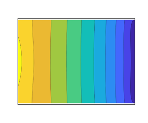
Figure 12(a–c) show the transverse profiles of pressure $p(0,y)$, density $\rho (0,y)$ and temperature $T(0,y)$ for three values of the Knudsen number ${Kn}=0.05$ (black line), $0.5$ (dashed magenta line) and $5$ (dot–dashed blue line), with $\delta p/p_0=1$ and other parameters as in figure 10. It is seen that while both the pressure and temperature profiles are of convex-up shape around the channel centreline, the density profiles are convex down at any ${Kn}$. All profiles become flatter with increasing ${Kn}$. For a comparison, we display the corresponding profiles of $(p(y), \rho (y), T(y))$ in figure 12(d–f) in the acceleration-driven Poiseuille flow for a dimensionless acceleration of $\hat {a}=0.1$.

Figure 12. Effects of Knudsen number on the cross-stream variations of (a) $p(x=0,y)$, (b) $\rho (0,y)$ and (c) $T(0,y)$ in pressure-driven Poiseuille flow with (a–c) $\delta p/p_0=1.0$. Panels (d–f) represent corresponding profiles in acceleration-driven Poiseuille flow with dimensionless acceleration $\hat {a}=0.1$; the inset in ( f) shows the close-up version of $T(y)$ for ${Kn}=0.05$, clarifying its ‘bimodal’ shape.

The first difference we encounter in figure 12 is about the shape of the temperature profile at small values of ${Kn}$: $T(y)$ at ${Kn}=0.05$ is of bimodal structure in the acceleration-driven flow (figure 12f), with a local minimum of temperature at $y=0$ and two local maxima symmetrically located away from the channel centre, in contrast to the convex-up temperature profiles that persist at all ${Kn}$ in its pressure-driven counterpart (figure 12c). The close-up version in the inset of figure 12( f) clearly identifies the locations of temperature minima and maxima for the case of ${Kn}=0.05$. The pressure profiles in figure 12(a,d) possess similar characteristic features as those of the temperature profiles in figure 12(c,f). It is known from theory (Tij & Santos Reference Tij and Santos1994; Uribe & Garcia Reference Uribe and Garcia1999; Tij & Santos Reference Tij and Santos2004; Rongali & Alam Reference Rongali and Alam2018a,Reference Rongali and Alamb) and simulations (Mansour et al. Reference Mansour, Baras and Garcia1997; Alam et al. Reference Alam, Mahajan and Shivanna2015; Gupta & Alam Reference Gupta and Alam2017, Reference Gupta and Alam2018) that the two local maxima in the $T(y)$-profile move towards the walls with increasing ${Kn}$, thereby making a transition from the bimodal-shape to unimodal convex-up shape for both $T(y)$ and $p(y)$ profiles in the acceleration-driven flow at large ${Kn}$.

The second difference between the two flows is that while the density profile $\rho (y)$ in the acceleration-driven flow has a minimum at the channel centre (see figure 12e), its pressure-driven counterpart admits a density maximum at $y=0$ in figure 12(b). The above differences regarding the role of forcing on the transverse profiles of ($p(y), \rho (y), T(y)$) persist when the imposed pressure gradient is reduced further, see figure 13. For example, the inset in figure 13(b) confirms the presence of the convex-down $\rho (y)$-profile even at $\delta p/p_0=0.1$ for ${Kn}=0.1$. Collectively, figures 12 and 13 underscore the qualitative differences in the shape of the temperature (and density) profiles, depending on whether the flow is generated by an axial pressure gradient or a constant acceleration.

Figure 13. Effects of imposed pressure gradient on cross-stream variations of (a) $p(x=0,y)$, (b) $\rho (0,y)$ and (c) $T(0,y)$ at ${Kn}=0.1$; Case A $\delta p/p_0=1$, Case B $\delta p/p_0=0.5$, Case C $\delta p/p_0=0.2$ and Case D $\delta p/p_0=0.1$, see table 3 for other parameters. Insets in (a–c) display the close-up version of the Case D.

3.2.2. Energy balance, pressure work and the absence of temperature bimodality

To check how the underlying assumptions in the two flows may impact the profiles of ($\rho (y), T(y), p(y)$), we consider the steady energy balance equation (in dimensionless form) at the NSF order,

(3.6)\begin{equation} \underline{ - \rho c_v \left( u_x\frac{\partial T}{\partial x} + u_y \frac{\partial T}{\partial y} \right) } - {\boldsymbol\nabla}\boldsymbol{\cdot} {\boldsymbol q} - \underline{ p({\boldsymbol\nabla}\boldsymbol{\cdot} {\boldsymbol u})} + \varPhi_{sh} =0, \end{equation}

in which the underlined terms ((i) convective heat transport and (ii) pressure work) are absent in the acceleration-driven Poiseuille flow, and the shear-work term

(3.7)\begin{equation} \varPhi_{sh} =2\mu\left( \left(\frac{\partial u_x}{\partial y}\right)^2 + \ldots\right) > 0 \end{equation}

is positive, representing the shear-induced heating of the gas. Next, we estimate the underlined terms in (3.6) at finite values of ${Kn}$ around the channel centreline ($y\sim 0$) to ascertain their relative importance compared with the shear work term. At the midchannel $y=0$, we have $u_y(x,0)=0$ and $\partial T/\partial x <0$ and hence the convective term simplifies to

(3.8)\begin{equation} Q_c = \left. - \rho c_v \left(u_x\frac{\partial T}{\partial x} + u_y \frac{\partial T}{\partial y} \right)\right|_{y=0} \equiv \left. - \frac{3}{2}\rho u_x(x,0)\left(\frac{\partial T}{\partial x}\right)\right|_{y=0} >0, \end{equation}

representing a heating effect; the pressure work is given by

(3.9)\begin{equation} \varPhi_p = \left. - p({\boldsymbol\nabla}\boldsymbol{\cdot}{\boldsymbol u})\right|_{y=0} < 0, \end{equation}

representing a cooling effect. Figure 14(a,b) verifies that $Q_c>0$ (figure 14a) and $\varPhi _p<0$ (panel b) in the bulk of the channel (except at the inlet and outlet of the channel). Furthermore, figure 14(c) confirms that the cooling due to pressure work (3.9) dominates over convective heating (3.8) at all ${Kn}$, resulting in a net cooling (i.e. $\varPhi _p+Q_c <0$) in the pressure-driven flow. These overall observations hold for transverse variations of $Q_c(0,y)$, $\varPhi _p(0,y)$ and $(\varPhi _p+Q_c)(0,y)$ too, see figures 14(d), 14(e) and 14( f), respectively. It is clear that the dominance of the pressure work over the convective heating is responsible for the cooling of the gas in the bulk of the channel – this leads to a lower bulk temperature in the pressure-driven case (viz. figure 12c) compared with its acceleration-driven counterpart (viz. figure 12f) at ${Kn}\to 0$. Consequently, the changes in the temperature profile affect the density and pressure profiles (via the equation of state $p=\rho T$) as demonstrated in figure 12(a,b,d,e). We conclude that the non-zero values of the terms in (3.8)–(3.9) in the pressure-driven flow are responsible for the different shapes of $(T(y), \rho (y))$ in the two flows even in the continuum limit of ${Kn} \to 0$ at finite values of $G_p$ and $\hat {a}$.

Figure 14. (a–c) Axial variations of (a) convective heat $Q_c$ (3.8), (b) pressure work $\varPhi _p$ (3.9) and (c) $(\varPhi _p+Q_c)$ at the midchannel ($y=0$) for different ${Kn}$, with $\delta p/p_0=1$ and $AR=3$. (d–f) Same as (a–c) but for transverse variations at $x=0$.

The foregoing analysis confirms that the absence of the bimodal shape of the temperature in the pressure-driven Poiseuille flow profile at small ${Kn}\sim 0$ is tied to the cooling afforded by the ‘pressure-dilatation’ work (3.9) which, however, vanishes in its acceleration-driven counterpart. It must be noted that the temperature bimodality has been predicted (Tij & Santos Reference Tij and Santos1994) to appear at the quartic order $O(a^4)$ in the acceleration-driven Poiseuille flow, however, the dilatation, $\varDelta =\boldsymbol {\nabla }\boldsymbol {\cdot }{\boldsymbol u}\sim O(G_p^2)$ (see § 3.3.1), also increases with increasing $G_p\propto \hat {a}$ in an equivalent pressure-driven flow. The increased dilatation would lead to a much lower bulk temperature due to the increased pressure-dilatation cooling, thereby further diminishing the possibility of temperature bimodality even in the nonlinear regime of forcing $O(\hat {a}^4)\sim O(G_p^4)$. Note that we did not observe bimodal temperature profile $T(y)$ when the pressure-gradient was changed by a factor of $10$ in present simulations. We conclude that the dilatation-driven pressure cooling ($\varPhi _p=-p\varDelta < 0$) is likely to be responsible for the absence of the bimodal-shape of $T(y)$ in the pressure-driven Poiseuille flow.

3.3. Are the pressure-driven and acceleration-driven Poiseuille flows equivalent?

It must be kept in mind that the Poiseuille flow of a molecular gas driven by a body force (acceleration) is an idealised, toy problem that cannot be realized in experiments. This forcing protocol was originally used by Cercignani & Daneri (Reference Cercignani and Daneri1963) in the context of solving the Boltzmann–BGK equation with a constant body force that yielded a steady and fully developed solution for a Poiseuille-type flow of a monatomic gas; this seminal work provided the first theoretical explanation of the Knudsen minimum phenomenon. Based on the present results in §§ 3.1–3.2, we note that while the ${Kn}$-dependence of the mass-flow rate in both acceleration-driven and pressure-driven flows looks similar (barring its scale dependence as in figure 8a), there exist key differences at the level of the hydrodynamic fields that can be appreciated by analysing the velocity gradient tensor of the two flows as discussed below.

3.3.1. Velocity gradient tensor, dilatation and the developing gaseous Poiseuille flow

The velocity gradient tensor is defined as

(3.10)\begin{equation} {\boldsymbol L} \stackrel{\text{def}}{=} ({\boldsymbol\nabla}{\boldsymbol u})^{\rm T} =\left[ \left(\frac{\partial u_j}{\partial x_i}\right)^{\rm T} \right]=\left[ \frac{\partial u_i}{\partial x_j}\right] =\left[ L_{ij}\right] = \left( \begin{array}{@{}ccc@{}} \dfrac{\partial u_x}{\partial x} & \dfrac{\partial u_x}{\partial y} & \dfrac{\partial u_x}{\partial z} \\ \dfrac{\partial u_y}{\partial x} & \dfrac{\partial u_y}{\partial y} & \dfrac{\partial u_y}{\partial z}\\ \dfrac{\partial u_z}{\partial x} & \dfrac{\partial u_z}{\partial y} & \dfrac{\partial u_z}{\partial z} \end{array} \right), \end{equation}

whose trace

(3.11)\begin{equation} {\mathrm{trace}}({\boldsymbol L}) = L_{kk} = \frac{\partial u_k}{\partial x_k}= \partial_k u_k \stackrel{\text{def}}{=} \varDelta \end{equation}

is called the dilatation. The symmetric part of $L_{ij}$ is

(3.12)\begin{equation} D_{ij} \stackrel{\text{def}}{=}\; \frac{1}{2}\left(L_{ij} + L_{ji}\right) =\frac{1}{2}\left( \frac{\partial u_i}{\partial x_j} + \frac{\partial u_j}{\partial x_i}\right) \end{equation}

and its deviatoric (traceless, symmetric) part is

(3.13)\begin{equation} S_{ij} = \overline{ {\partial_j u_i}} \;\stackrel{\text{def}}{=}\; \frac{1}{2}\left( \frac{\partial u_i}{\partial x_j} + \frac{\partial u_j}{\partial x_i}\right) - \frac{1}{3}\delta_{ij}\frac{\partial u_k}{\partial x_k} \equiv D_{ij} - \frac{\varDelta}{3}\delta_{ij} =S_{ji}, \end{equation}

denoted by an ‘over-bar’ on the respective tensorial quantity. The deformation field is classified in terms of the invariants of the objective deformation rate ${\boldsymbol D}$, defined via $D_k=trace({\boldsymbol D}^k)/k,~k=1,2,3$ (Goddard Reference Goddard2014), with the dilatation $\varDelta ={\rm trace}({\boldsymbol D})\equiv D_1$ being its first invariant. The dilatation-free, $\varDelta =0$, deformation for a compressible gas is equivalent to the condition that the material derivative of the mass density is zero,

(3.14)\begin{equation} \frac{{\rm D}\rho}{{\rm D}t} \equiv \left(\frac{\partial}{\partial t} + {\boldsymbol u}\boldsymbol{\cdot}{\boldsymbol\nabla}\right)\rho ={-}\rho({\boldsymbol\nabla}\boldsymbol{\cdot}{\boldsymbol u}) =0, \end{equation}

i.e. the specific-volume ($v=1/\rho$) is preserved, and such deformation field ($D\rho /Dt=0$) is known as ‘isochoric’ (volume preserving) deformation.

For the present case of steady, pressure-driven Poiseuille flow, there are no gradients along the $z$-direction, i.e. ${\boldsymbol u}(x,y)= (u_x, u_y, 0)(x,y)$ with $\partial /\partial z({\cdot })=0$, and hence the velocity gradient tensor and its symmetric part are

(3.15a,b)\begin{align} {\boldsymbol L} = \left( \begin{array}{@{}ccc@{}} \dfrac{\partial u_x}{\partial x} & \dfrac{\partial u_x}{\partial y} & 0 \\ \dfrac{\partial u_y}{\partial x} & \dfrac{\partial u_y}{\partial y} & 0 \\ 0 & 0 & 0 \end{array} \right) \quad \text{and} \quad {\boldsymbol D} = \left( \begin{array}{@{}ccc@{}} \dfrac{\partial u_x}{\partial x} & \dfrac{1}{2}\left(\dfrac{\partial u_x}{\partial y} +\dfrac{\partial u_y}{\partial x}\right) & 0\\ \dfrac{1}{2}\left(\dfrac{\partial u_x}{\partial y} +\dfrac{\partial u_y}{\partial x}\right) & \dfrac{\partial u_y}{\partial y} & 0 \\ 0 & 0 & 0 \end{array} \right), \end{align}

with its deviatoric part being

(3.16)\begin{equation} {\boldsymbol S} = \left( \begin{array}{@{}ccc@{}} \dfrac{\partial u_x}{\partial x} -\dfrac{\varDelta}{3} & \dfrac{1}{2}\left(\dfrac{\partial u_x}{\partial y} +\dfrac{\partial u_y}{\partial x}\right) & 0\\ \dfrac{1}{2}\left(\dfrac{\partial u_x}{\partial y} +\dfrac{\partial u_y}{\partial x}\right) & \dfrac{\partial u_y}{\partial y} - \dfrac{\varDelta}{3} & 0\\ 0 & 0 & -\dfrac{\varDelta}{3} \end{array} \right) . \end{equation}

An expression for the dilatation and its scaling can be obtained by noting the fact that the steady pressure-driven Poiseuille flow of a gas can never be in a fully developed state, irrespective of the channel length ($L_x< \infty$), and hence the flow field is two-dimensional (viz. figures 5a,b, 6a,b and 9; assuming homogeneity along the $z$-direction). The latter can be understood from the steady mass balance equation (3.1):

(3.17)$$\begin{gather} \Delta(x,y) = {\boldsymbol\nabla}\boldsymbol{\cdot}{\boldsymbol u} ={-} u_x\frac{\partial\ln\rho}{\partial x} - u_y\frac{\partial\ln\rho}{\partial y}, \end{gather}$$

(3.18)$$\begin{gather}\Rightarrow\quad \Delta(x,0) ={-} u_x(x,0)\left. \frac{\partial\ln\rho}{\partial x}\right|_{y=0} \neq 0. \end{gather}$$

Equation (3.18) implies that the local dilatation is always finite and positive since (i) $u_x(x,0)>0$ and (ii) the density of the gas decreases along the axial direction (viz. figures 10b and 11b), irrespective of (i) the magnitude of the axial pressure gradient $G_p$ and (ii) the length of the channel ($L_x$). For the pressure-driven flow,

(3.19a,b)\begin{equation} u_x\propto \frac{{\rm d}p}{{\rm d}{\kern0.7pt}x}=\frac{\delta p}{L_x} \sim G_p \quad \text{and} \quad \rho=\rho_0(1-G_\rho x - G_\rho^2 x^2), \end{equation}

and assuming that $G_\rho =O(G_p)$ under small pressure gradient, it immediately follows that

(3.20)\begin{equation} \Delta(x,0) \sim G_p G_\rho \sim G_p^2, \end{equation}

i.e. the dilatation scales quadratically with the imposed pressure-gradient $G_p$.

That the dilatation is non-zero within the bulk of the channel can be ascertained from figure 15(a,b) that display the contours of $\Delta (x,y)/G_p^2$ for ${{Kn}}=0.05$ and $0.5$, respectively; the imposed pressure gradient is $G_p=1/15$ (i.e. $\delta p/p_0=0.2$) and the channel aspect ratio is $AR=3$. Similar qualitative variations of $\Delta (x,y)$ hold also in longer channels with $AR=9$ and $27$ (not shown). Figure 15(c,d) confirms that $\Delta (x,0)>0$ and increases axially within the bulk region of the channel, except near the entrance and exit, irrespective of the values of the channel length ($L_x$) and the pressure gradient ($G_p$). It is also clear from figure 15(c,d) that the quadratic scaling (3.20) holds approximately within the bulk of the channel, and the data collapse is relatively better at higher rarefaction (${{Kn}}= 0.5$, figure 15d) than that at ${{Kn}}= 0.05$ (figure 15c). The case denoted by the black line in figure 15(c) corresponds to a nonlinear axial density profile (see the profile of $\partial _x\rho (x,0)$ in figure 15e) and the neglected HOT (i.e. $\partial _x\rho (x,0)= -G_\rho - G_\rho ^2 x + \cdots$) are likely responsible for its disagreement with the remaining two cases in figure 15(c) for ${{Kn}}=0.05$. On the other hand, the density profiles $\rho (x,0)$ at higher rarefaction (${{Kn}}=0.5$) can be approximated having a linear decay with $x$, with nearly constant axial gradients (see figure 15f), and hence the axial profiles of $\Delta (x,0)/G_p^2$ for the three cases at ${{Kn}}=0.5$ closely follow each other in figure 15(d).

Figure 15. (a,b) Contours of the normalized dilatation ‘$\Delta (x,y)/G_p^2$’ in the ($x/L_y, y/L_y$)-plane for $G_p=1/15$ ($\delta p/p_0=0.2$) and $AR=3$. (c,d) Axial variations of ‘$\Delta (x,0)/G_p^2$’ for three data sets: (i) black solid line ($G_p=1/3$ (i.e. $\delta p/p_0=1.0$) and $AR=3$); (ii) blue dashed line ($G_p=1/15$ ($\delta p/p_0=0.2$) and $AR=3$); (iii) red dot–dashed line ($G_p=1/15$ ($\delta p/p_0=0.6$) and $AR=9$). (e,f) Axial variations of the density gradient ‘$\partial \rho (x,0)/\partial x$’, with other parameters as in panels (c,d). The panels denote data for (a,c,e) ${{Kn}}=0.05$ and (b,d,f) ${{Kn}}=0.5$, respectively. The wiggles seen in two data sets in (c,d) are due to (i) the discrete derivative calculations and (ii) the increased noise in the DSMC data at small values of $G_p$.

For the idealized problem of the acceleration-driven Poiseuille flow (Cercignani & Daneri Reference Cercignani and Daneri1963; Ohwada et al. Reference Ohwada, Sone and Aoki1989; Alaoui & Santos Reference Alaoui and Santos1992; Tij & Santos Reference Tij and Santos1994; Mansour et al. Reference Mansour, Baras and Garcia1997; Uribe & Garcia Reference Uribe and Garcia1999; Aoki et al. Reference Aoki, Takata and Nakanishi2002; Gupta & Alam Reference Gupta and Alam2017; Rongali & Alam Reference Rongali and Alam2018a; Alam et al. Reference Alam, Gupta and Ravichandir2021) of a gas, the flow is one-dimensional with no gradients along $x$ and $z$-directions, i.e. ${\boldsymbol u}(y)= (u_x(y), 0, 0)$ with $\partial /\partial x({\cdot })=0=\partial /\partial z({\cdot })$. The velocity gradient tensor and its symmetric and deviatoric parts are given by

(3.21a,b)\begin{equation} {\boldsymbol L} = \left( \begin{array}{@{}ccc@{}} 0 & \dfrac{\partial u_x}{\partial y} & 0 \\ 0 & 0 & 0 \\ 0 & 0 & 0 \end{array} \right) \quad \text{and}\quad {\boldsymbol D} = \left( \begin{array}{@{}ccc@{}} 0 & \dfrac{1}{2}\dfrac{\partial u_x}{\partial y} & 0 \\ \dfrac{1}{2}\dfrac{\partial u_x}{\partial y} & 0 & 0 \\ 0 & 0 & 0 \end{array} \right) \equiv {\boldsymbol S} . \end{equation}

The dilatation is given by

(3.22)\begin{equation} \Delta(x,y,z) = \frac{\partial u_x}{\partial x} + \frac{\partial u_y}{\partial y} + \frac{\partial u_z}{\partial z} =0, \end{equation}

i.e. the steady, fully developed acceleration-driven Poiseuille flow is divergence-free and consequently the deformation is isochoric (${\rm D}\rho /{\rm D}t=0$) which remains the major difference with its non-isochoric (${\rm D}\rho /{\rm D}t\neq 0$) pressure-driven counterpart (3.20) at the level of the velocity gradient tensor.

4.1. Shear stress and viscosity

Using the DSMC data on the shear stress $P_{xy}$, the local shear viscosity is calculated from

(4.2)\begin{equation} \mu(x,y) ={-} \frac{P_{xy}(x,y)}{2 S_{xy}}, \end{equation}

where $2S_{xy}=\dot \gamma (x,y)=(\partial _y u_x + \partial _x u_y)\approx \partial _y u_x$ is the local shear rate. The cross-stream variations of the shear stress $P_{xy}(0,y)$, the local shear rate $\dot \gamma (0,y)$ and the shear viscosity $\mu (0,y)$ for different ${Kn}$ are shown in figures 16(a), 16(b) and 16(c), respectively, for $\delta p/p_0=1$ and $AR=3$; the analogous plots for the acceleration-driven flow are displayed in figure 16(d–f) for $\hat {a}=0.1$. It is seen in figure 16(a,d) that the shear stress $P_{xy}(y)$ profiles are nearly linear with $y$ and independent of ${Kn}$ at large values of ${Kn}$ for both forcing, but become nonlinear with $y$ at small values of ${Kn}$ (${Kn} = 0.05$, figure 16a) for the pressure-driven case. From the viscosity variations in figure 16(c,f), we find that the viscosity decreases away from the channel centreline ($y=0$), confirming the shear-thinning behaviour of rarefied gases since the local shear rate $\dot {\gamma }(0,y)$ (see figure 16b,e) increases in the same limit. Note further in figure 16(c,f) that the viscosity profiles become increasingly non-uniform with increasing ${Kn}$, and the magnitude of local $\mu (y)$ increases with increasing ${Kn}$ due to the decrease in the overall/effective shear rate (across the half-channel width),

(4.3)\begin{equation} \dot{\gamma}_{eff} = \frac{u_x(0) -u_x ({\pm} 1/2)}{L_y/2} \equiv \frac{1}{2}\left(\frac{{\rm d}u_x}{{\rm d} y}(y={-}0.5) + \frac{{\rm d}u_x}{{\rm d} y}(y=0.5)\right) \end{equation}

as in figure 16(b,e).

Figure 16. (a–c) Cross-stream variations of (a) shear stress $P_{xy}(0,y)$, (b) shear rate ${\rm d}u_x/{{\rm d} y}(0,y)$ and (c) shear viscosity $\mu (0,y)$ at $x=0$ in pressure-driven Poiseuille flow with $\delta p/p_0=1$ and $AR=3$. (d–f) Same as in (a–c), but for the acceleration-driven case with dimensionless acceleration $\hat {a} = 0.1$. The insets in (c,f) denote the close-up version of the case with ${Kn}=0.05$. For all panels the channel width is $L_y/d=1860$.

We define the ‘width-averaged’ shear viscosity

(4.4)\begin{equation} \mu_{av} = \int_{{-}1/2}^{1/2} \mu(0,y) \,{{\rm d} y}, \end{equation}

as a measure for the effective flow resistance in the bulk. Figure 17(a) illustrates the effect of imposed pressure gradient on $\mu _{av}(x=0)$ for $\delta p/p_0=1$ and $0.2$; both curves closely follow each other, before settling towards a plateau value at ${Kn}\gg 1$, similar to the saturation of the mass flow rate seen in figure 8(a). Figure 17(b) indicates that the saturation of $\mu _{av}$ at large ${Kn}$ is a consequence of the finite length of the channel. Comparing figure 17(a) with figure 17(c), we find that the average viscosity in the pressure-driven case is smaller than that in its acceleration-driven counterpart. This observation holds also for the local viscosity $\mu (y)$ as it is evident from figure 16(c,f).

Figure 17. Variations of the width-averaged viscosity $\mu _{av}(x=0)$ (4.4) with Knudsen number: (a) effect of pressure gradient ($\delta p/p_0=1$, open black circles; $\delta p/p_0=0.2$, filled blue circles) on $\mu _{av}$ for $AR=3$ (table 3); (b) effect of channel length/aspect-ratio on $\mu _{av}$ for $\delta p/p_0=0.2$ (table 2). (c) Acceleration-driven flow with $\hat {a}=0.1$. For all panels the channel width is $L_y/d=1860$.

To explain the above finding of the reduction of viscosity, we consider the leading expression for the shear-viscosity of a gas undergoing pressure-driven Poiseuille flow,

(4.5)\begin{equation} \mu = \mu_{{NSF}}{\mathcal{F}}_0(\varDelta, T), \quad \text{with} \ {\mathcal{F}}_0(\varDelta,T) \approx 1 - c_\mu\, {{Kn}} \left(\frac{\varDelta}{\sqrt{T}} \right), \end{equation}

valid up-to the Burnett-order $O({{Kn}}^2)$, where

(4.6)\begin{equation} \mu_{{NSF}}=\mu_0\sqrt{T}, \quad \text{with} \ \mu_0=\sqrt{2}\omega_0\rho l_f \approx 0.7957\rho l_f, \end{equation}

denotes the viscosity at the NSF order and ${\mathcal {F}}_0(\varDelta,T)$ is its Burnett-order correction factor, with $c_\mu \approx 4$; (4.5) holds strictly around the channel centreline, see Appendix C.2 for details. The dimensionless expression ${\mathcal {F}}_0(\varDelta, T)$ in (4.6) incorporates the leading correction due to finite dilatation ($\varDelta \neq 0$), a characteristic of the pressure-driven gaseous Poiseuille flow. It should be noted that for the isochoric deformation ($\varDelta =0$) of a monatomic gas the expressions for the shear viscosity (Chapman & Cowling Reference Chapman and Cowling1970; Saha & Alam Reference Saha and Alam2020) at the NSF and Burnett orders are identical (i.e. $\mu _{{NSF}}=\mu _{{Burnett}}$).

For a quantitative understanding, with parameter values of ${Kn}=0.05$, $\delta p=p_0$, and $AR=3$, it has been verified that, at the middle $(x,y)=(0,0)$ of the channel,

(4.7)\begin{equation} \frac{\partial u_x}{\partial x} \approx 20\left(\frac{\partial u_y}{\partial y}\right), \quad \Rightarrow \Delta(0,0) \approx \left. \frac{\partial u_x}{\partial x}\right|_{(0,0)} \approx 0.096. \end{equation}

With (4.7), the estimated shear viscosity (4.5) is

(4.8)\begin{equation} \mu(0,0) \approx 0.9817\mu_0\sqrt{T}, \end{equation}

a reduction of less than $2\,\%$, compared with its value ($\mu (0)=\mu _0 \sqrt {T}=\mu _{{Burnett}}\equiv \mu _{{NS}}$) in the acceleration-driven Poiseuille flow. Note that the positivity of the dilatation holds in the bulk region of the channel (i.e. $\Delta (x,y)>0$), except near its entrance and exit, see figure 15(a–d). Therefore, we conclude that the effect of the dilatation/non-isochoricity is to reduce the shear viscosity (4.5) of the gas in the pressure-driven Poiseuille flow.

4.2. Normal stress differences

In general, the diagonal components of the stress tensor (4.1) are unequal (i.e. $P_{xx}\neq P_{yy}\neq P_{zz}$), and hence, in addition to pressure $p=P_{ii}/3$ and shear stress $P_{xy}$, two independent quantities are needed to completely describe the stress tensor in Poiseuille-type flows. These two functions are defined as (Sela & Goldhirsch Reference Sela and Goldhirsch1998; Alam & Luding Reference Alam and Luding2003, Reference Alam and Luding2005)

(4.9a,b)\begin{equation} {\mathcal{N}}_1(x,y) = \frac{P_{xx} - P_{yy}}{p} \quad \text{and} \quad {\mathcal{N}}_2(x,y) = \frac{P_{yy}- P_{zz}}{p} \equiv \frac{P_{xx} + 2P_{yy}}{p} -3 , \end{equation}

known as the first (primary) and second (secondary) normal stress differences, respectively. The contour plots of $\mathcal {N}_1(x,y)$ and $\mathcal {N}_2(x,y)$ are shown in figure 18(a,b) for ${Kn}=0.05$, indicating strong variations of both quantities along the axial and transverse directions in the pressure-driven Poiseuille flow.

Figure 18. Contour plots of (a) $\mathcal {N}_1(x,y)$ and (b) $\mathcal {N}_2(x,y)$ for ${Kn}=0.05$, $\delta p/p_0=1$ and $AR=3$ ($L_y/d=1860$).

The cross-stream variations of $\mathcal {N}_1(0,y)$ and $\mathcal {N}_2(0,y)$, both evaluated at $x=0$, are shown in figures 19(a) and 19(b), respectively. It is seen that $\mathcal {N}_1$ is an order of magnitude larger compared with $\mathcal {N}_2$, and in general the two normal stress differences are found to be of opposite signs, for example,

(4.10a,b)\begin{equation} \mathcal{N}_1<0 \quad \text{and}\quad \mathcal{N}_2>0, \end{equation}

at any ${Kn}$ in the pressure-driven case. Comparing the variations of $\mathcal {N}_1 (0,0)$ and $\mathcal {N}_2 (0,0)$ with the Knudsen number in figure 20(a,b), we find that the magnitudes of both quantities increase with increasing ${Kn}$. The observation of the anticorrelation between $\mathcal {N}_1$ and $\mathcal {N}_2$ is similar to the theoretical (Rongali & Alam Reference Rongali and Alam2018a,Reference Rongali and Alamb) and previous numerical (Gupta & Alam Reference Gupta and Alam2017) findings in the acceleration-driven Poiseuille flow as well as in simple shear flow (Sela & Goldhirsch Reference Sela and Goldhirsch1998; Alam & Luding Reference Alam and Luding2005; Saha & Alam Reference Saha and Alam2016). For the sake of comparison, the corresponding plots for the acceleration-driven case are displayed in figures 19(c,d) and 20(c,d) for a dimensionless acceleration of $\hat {a}=0.1$; it is seen that while $\mathcal {N}_1(y)$ remains positive and increases with increasing ${Kn}$, the variation of $\mathcal {N}_2(y)$ with ${Kn}$ is found to be non-monotonic; in particular, $\mathcal {N}_2(0)$ (figure 20d) is negative over a range of ${Kn}<10$ but attains a positive value at large ${Kn}>10$. Comparing figures 20(a) and 20(c), we find that

(4.11a,b)\begin{equation} \mathcal{N}_1(0,0)|_{{pressure\text{-}driven}} < 0 \quad \text{and} \quad \mathcal{N}_1(0)|_{{acceleration\text{-}driven}} > 0, \quad \forall \ {Kn}>0. \end{equation}

This sign-reversal also holds for the second normal stress difference (figure 20b,d),

(4.12a,b)\begin{align} \left. \mathcal{N}_2(0,0)\right|_{{pressure\text{-}driven}} > 0 \quad \text{and} \quad \left. \mathcal{N}_2(0)\right|_{{acceleration\text{-}driven}} < 0 \quad \text{at}\ {Kn}< O(10), \end{align}

but both $\mathcal {N}_2(0,0)$ and $\mathcal {N}_2(0)$ attain positive values at large enough ${Kn}>10$.

Figure 19. Cross-stream variations of (a) $\mathcal {N}_1(0,y)$ and (b) $\mathcal {N}_2(0,y)$, respectively, at the midchannel $x=0$ in the pressure-driven flow, with parameter values as in figure 18. (c,d) Analogues of (a,b) for acceleration-driven flow with $\hat {a} = 0.1$. For all panels the channel width is $L_y/d=1860$.

Figure 20. Variations of (a) $\mathcal {N}_1(0,0)$ and (b) $\mathcal {N}_2(0,0)$ with Knudsen number in the pressure-driven flow with parameter values as in figure 18. (c,d) Analogues of (a,b) for the acceleration-driven flow with $\hat {a} = 0.1$. For all panels the channel width is $L_y/d=1860$.

The above findings on the ${Kn}$-dependence of two normal stress differences are robust, irrespective of the value of the imposed pressure gradient and the channel length as confirmed in figure 21(a,b). It is seen that the magnitude of $\mathcal {N}_1(0,0)$ decreases with decreasing $G_p$, and tends to saturate to constant values at large ${Kn}\gg 1$, irrespective of the imposed pressure gradient; similar behaviour persists for $\mathcal {N}_2(0,0)$ too (not shown).

Figure 21. Effects of (a) imposed pressure gradient and (b) channel length or aspect-ratio on the variations of $\mathcal {N}_1(0,0)$ with Knudsen number. For both panels, the channel width is $L_y/d=1860$, with other parameters as in tables 2 and 3.

4.3. Origin of normal stress differences and comparison with theory

The sign-change of two normal stress differences ((4.11a,b)–(4.12a,b)), depending on whether the flow is generated by an axial pressure gradient or a constant body force, is one major difference between the two Poiseuille-type flows. To provide a theoretical justification for the observed differences in (4.11a,b)–(4.12a,b), we carry out an analysis at the channel centre $(x,y)=(0,0)$ for which

(4.13)\begin{equation} \left. \frac{\partial}{\partial y}(\rho, T, p, u_x)\right|_{y=0} =0 \end{equation}

that holds for both the forcings.

4.3.1. Origin of ${\mathcal {N}}_i$ and the inequivalence between the two flows

From the Burnett-order $O({Kn}^2)$ stress tensor (Chapman & Cowling Reference Chapman and Cowling1970; Sela & Goldhirsch Reference Sela and Goldhirsch1998), the expressions for two normal stress differences have been derived – the details are given in Appendix C.3, leading to (C21) and (C23). For the pressure-driven Poiseuille flow, the expressions for the first and second normal stress differences, evaluated at $(x,y)=(0,0)$, are given by

(4.14)$$\begin{gather} {\mathcal{N}}_1(0,0) \approx {{Kn}}^2\left( c_1 p^{{-}1} \partial_{yy}p - (c_1-c_2) T^{{-}1} \partial_{yy}T \right) -\frac{2\mu(T,\varDelta)}{p}\, {\mathcal{S}}_1 \nonumber\\ \underline{ - c_3 {{Kn}}^2 p^{{-}1} \partial_x T\partial_x \rho + c_4 {{Kn}}^2 T^{{-}2} (\partial_x T)^2 - c_5 {{Kn}}^2 T^{{-}1}{\mathcal{S}}_1\varDelta }\; , \\ {\mathcal{N}}_2(0,0) ={-} {{Kn}}^2\left( c_1 p^{{-}1} \partial_{yy} p - (c_1 - c_2)T^{{-}1} \partial_{yy} T \right) -\frac{2\mu(T,\varDelta)}{p} {\mathcal{S}}_2 \nonumber \end{gather}$$

(4.15)$$\begin{gather}\underline{- {{Kn}}^2T^{{-}1}\left( c_6 \varDelta - c_7 {\mathcal{S}}_2\right) {\mathcal{S}}_2 } \; , \end{gather}$$

where the numerical constants, $c_i$, are

(4.16a–e)\begin{equation} c_1\approx 3.8532,\quad c_2 \approx 2.322,\quad c_3 \approx 2.1374, \quad c_4\approx 0.57, \quad c_5 \approx 0.1452, \end{equation}

and

(4.17)$$\begin{gather} {\mathcal{S}}_1 \stackrel{\text{def}}{=} \left({S}_{xx} - {S}_{yy}\right) = \frac{\partial u_x}{\partial x} - \frac{\partial u_y}{\partial y} \equiv D_{xx} - D_{yy} , \end{gather}$$

(4.18)$$\begin{gather}{\mathcal{S}}_2 \stackrel{\text{def}}{=} \left({S}_{yy} - {S}_{zz}\right) = \frac{\partial u_y}{\partial y} - \frac{\partial u_z}{\partial z} = \frac{\partial u_y}{\partial y} \equiv D_{yy} - D_{zz} , \end{gather}$$

are called the first and second normal shear-rate difference (NSRD), respectively. The latter two parameters ((4.17)–(4.18)) represent the diagonal-anisotropy of the deformation rate ${\boldsymbol D}$ and its deviator ${\boldsymbol S}$ that are defined in § 3.3.1. Note that while the expression for ${\mathcal {N}}_2(0,0)$ in (4.15) is exact at this level, $O({{Kn}}^2)$, of analysis, (4.14) has been approximated via an additional assumption that $\partial _{xx}(\rho, T) \ll \partial _{yy}(\rho, T)$ (see Appendix C.3).

The second term ($\propto {\mathcal {S}}_i$) in each of (4.14)–(4.15) needs clarification: they can be identified with the second and third terms in (C1), or, equivalently, with the second term in (C5) of the stress tensor, and are also present in the NSF-order $O({{Kn}})$ constitutive relation for the stress tensor. For finite values of $G_p$ and ${\mathcal {S}}_i$, the quadratic-order terms in ${{Kn}}$ in (4.14)–(4.15) can be neglected for ${{Kn}}\to 0$ and hence the expressions for ${\mathcal {N}}_i(0,0)$ simplify to

(4.19)\begin{equation} {\mathcal{N}}_i(0,0) \stackrel{{{Kn}}\to 0}{=} -\frac{2\mu}{p}{\mathcal{S}}_i = O\left({{Kn}}{\mathcal{S}}_i \right), \quad \text{with} \ i=1,2, \end{equation}

since $\mu /p=O({{Kn}})$, and the sign of ${\mathcal {N}}_i(0,0)$ is dictated by ‘${\mathrm {sgn}}(-{\mathcal {S}}_i)$’ at ${{Kn}}\to 0$. Therefore, we conclude that the normal stress differences appear at $O({{Kn}})$ in the pressure-driven gaseous Poiseuille flow, both being driven by the coupling between the dynamic friction ($\mu /p$) and the NSRDs (${\mathcal {S}_i}\neq 0$). This should be contrasted with the Burnett-order $O({{Kn}}^2)$ origin (Sela & Goldhirsch Reference Sela and Goldhirsch1998; Alam & Luding Reference Alam and Luding2005; Saha & Alam Reference Saha and Alam2016) of the normal stress differences in the idealized acceleration-driven Poiseuille flow (Gupta & Alam Reference Gupta and Alam2017; Rongali & Alam Reference Rongali and Alam2018a) for which both the NSRDs vanish (${\mathcal {S}}_1=0={\mathcal {S}}_2$). Equation (4.19) provides a confirmation of our assertion in § 3.3.2 that the pressure-driven and acceleration-driven Poiseuille flows are not equivalent even at NSF order $O({{Kn}})$.

4.3.2. Qualitative comparison between theory and simulation

It follows from (3.19a,b)–(3.20) and (4.17)–(4.18) that

(4.20)\begin{equation} {\mathcal{S}}_1= O\left(G_p^2\right) \end{equation}

is second order in the normalized pressure-gradient ($G_p$), and ${\mathcal {S}}_2= O(G_p^2/AR) \ll {\mathcal {S}}_1$. The underlined terms in each of (4.14)–(4.15) are smaller compared with the terms in the respective first line if the streamwise gradients of the hydrodynamic fields are assumed to be smaller than their transverse gradients. This has been verified from the present simulation data at ${Kn}=0.05$ and $0.5$ with $G_p=1/3$; more specifically, the sum of the underlined terms in (4.14)–(4.15) remains negative and is an order-of-magnitude smaller than the third ($\propto {\mathcal {S}}_i$, negative) term in the corresponding equation, and hence they can be neglected. Therefore, the leading expressions for ${\mathcal {N}}_i(0,0)$ simplify to

(4.21)$$\begin{gather} {\mathcal{N}}_1(0,0) \approx{-}\frac{2\mu(T,\varDelta)}{p}\, {\mathcal{S}}_1 \underbrace{ - (c_1-c_2) {{Kn}}^2 T^{{-}1} \partial_{yy}T + c_1 {{Kn}}^2{p}^{{-}1} \partial_{yy}p } , \end{gather}$$

(4.22)$$\begin{gather}{\mathcal{N}}_2(0,0) \approx (c_1-c_2) {{Kn}}^2 T^{{-}1}\partial_{yy} T \underbrace{- c_1{{Kn}}^2 p^{{-}1}\partial_{yy} p -\frac{2\mu(T,\varDelta)}{p} {\mathcal{S}}_2 }. \end{gather}$$

At this level of analysis, there is a competition between the Burnett-order ($\propto {{Kn}}^2$) and the NSF-order ($\propto {\mathcal {S}}_i$) terms that would decide the sign of the two normal stress differences, depending on the values of imposed pressure gradient ($G_p$) and the Knudsen number (${{Kn}}$). While the rarefaction-induced terms in (4.21)–(4.22) dominate in the limit of $G_p\to 0$, the dilatation-driven terms dominate in the continuum limit ${{Kn}}\to 0$. In principle, one can determine a threshold value of ${{Kn}}_c(G_p)$ for finite $G_p$ that would help to identify two regions in the ($G_p, {{Kn}})$-plane where the dilatation and rarefaction effects are dominant. A complete analysis would require numerically evaluating the gradients of ($p, T$) for given ($G_p, {{Kn}})$, and is beyond the scope of the present paper. Below we focus on a few specific parameter values of ($G_p, {{Kn}}$) to estimate the order of magnitudes of different terms in (4.21)–(4.22) and comment on the leading behaviour of ${\mathcal {N}}_i(0,0)$ over the studied range of $G_p$.

From the simulation data in figure 12(a,c) for ${Kn}=0.05$, we have evaluated the curvature terms to be ordered as

(4.23)\begin{equation} \partial_{yy}T(0) \sim 10 \partial_{yy}p(0) \gg \partial_{yy}p(0) >0, \end{equation}

and the NSRDs are approximated as

(4.24a,b)\begin{equation} \left. {\mathcal{S}}_1(0,0)\right|_{{Kn}=0.05}\approx 10^{{-}1} \quad \text{and} \quad \left. {\mathcal{S}}_2(0,0)\right|_{{Kn}=0.05}\approx 5\times 10^{{-}3}. \end{equation}

The sum of the two under-braced terms in (4.21) is found to be negative (but its magnitude is smaller by a factor of 10 compared with the first term), and hence the leading expression is

(4.25)\begin{equation} {\mathcal{N}}_1(0,0) \sim{-}\frac{2\mu(T,\varDelta)}{p} {\mathcal{S}}_1 < 0 , \end{equation}

in agreement with simulation results in figure 20(a). It has been verified from present simulations that the above estimates hold also at ${Kn}=0.5$, and therefore the behaviour of ${\mathcal {N}}_1(0,0)$ is dictated by (4.25). Note that (4.25) represents the correlation between the first NSRD ${\mathcal {S}}_1$ and the dynamic friction $\mu (T,\varDelta )/p$ which is the leading expression of ${\mathcal {N}}_1(0,0)$ and hence responsible for its negative sign in the pressure-driven flow.

On the other hand, using the simulation data at ${Kn}=0.05$ and $0.5$, we found that the sum of the under-braced terms in (4.22) remains negative, but is of smaller magnitude compared with the first term which is positive, leading to

(4.26)\begin{equation} {\mathcal{N}}_2(0,0) \sim (c_1-c_2) \frac{{{Kn}}^2}{T} \partial_{yy} T > 0. \end{equation}

Therefore, the positive sign of ${\mathcal {N}}_2(0,0)$ is primarily dictated by the curvature in the temperature field at the channel centre. Recalling from § 3.2.2 that the curvature in $T(y)$ is strongly influenced by the dilatation-coupled pressure cooling, the behaviour of the second normal stress difference is also tied indirectly to dilatation-driven effects. On the whole, our Burnett-order analysis correctly predicts the signs of both ${\mathcal {N}}_1(0,0)$ and ${\mathcal {N}}_2(0,0)$ for small ${Kn}$ in the pressure-driven Poiseuille flow.

For the acceleration-driven Poiseuille flow, we have

(4.27)\begin{equation} \varDelta=0={\mathcal{S}}_i=\partial/\partial x({\cdot}), \end{equation}

and hence it follows from (4.14)–(4.15) that

(4.28)$$\begin{gather} {\mathcal{N}}_1(0) = c_1 {{Kn}}^2 p^{{-}1} \partial_{yy} p -(c_1-c_2) {{Kn}}^2 T^{{-}1}\partial_{yy} T , \end{gather}$$

(4.29)$$\begin{gather}{\mathcal{N}}_2(0) ={-} {\mathcal{N}}_1(0) , \end{gather}$$

with $c_i$ given in (4.16a–e). From the simulation data in figure 12(d,f), it has been verified that

(4.30a,b)\begin{equation} \partial_{yy}p(0)> \partial_{yy}T(0) >0 \quad \text{and}\quad \partial_{yy}p(0) =O\left( \partial_{yy}T(0)\right), \end{equation}

for small values of ${Kn}$ – this balance of curvature terms in (4.30a,b) should be contrasted with (4.23) that hold for its pressure-driven counterpart which is strongly influenced by the dilatation. It follows immediately from (4.28)–(4.29) that ${\mathcal {N}}_1(0) >0$ and ${\mathcal {N}}_2(0)< 0$ at the middle of the channel – these predictions are in qualitative agreement with the DSMC results in figure 20(c,d) for the acceleration-driven flow. Note, however, that there is another sign-change of $\mathcal {N}_2(0)$ (from negative to positive values, see figure 20d) at large values of ${Kn}=O(10)$ – this remains unexplained since the Burnett-order theory $O({Kn}^2)$ is likely to hold only at small values of ${Kn} < 1$.

To conclude this section, the ${Kn}$-dependence of ${\mathcal {N}}_1(0,0)$ and ${\mathcal {N}}_2(0,0)$ (figures 20a,b and 20c,d) and their signs at small ${Kn}$ are dictated by (i) the dilatation-driven effects (i.e. the NSRD-dynamic-friction coupling (4.25) and the pressure-dilatation cooling) in the pressure-driven Poiseuille flow and (ii) the curvatures in temperature and pressure/density profiles in its acceleration-driven counterpart.

5.1. Normal and tangential heat fluxes

Figure 22(a) displays the cross-stream variations of the normal heat flux $q_y(0,y)$ at the midchannel ($x=0$) for a range of Knudsen number. Comparing them with their acceleration-driven flow counterparts in figure 22(c), we find that the direction of $q_y(0,y)$ is reversed which is now directed from the walls towards the channel centre. This can be understood from the temperature profiles in figure 12(c,f) along with Fourier's law of heat conduction (5.1). The corresponding profiles of the tangential heat-flux $q_x(x=0,y)$ are displayed in figure 22(b,d). For the pressure-driven case, a double-well-shaped $q_x(0,y)$ profile is found at small values of ${Kn}$ ($=0.01$ and $0.05$, see figure 22b) that transitions into a single-well structure with increasing Knudsen number; in contrast, $q_x(y)$ profiles are of single-well shape for all ${Kn}>0$ in the acceleration-driven flow, see figure 22(d).

Figure 22. Cross-stream variations of (a,c) normal heat flux $q_y(0,y)$ and (c,d) tangential heat flux $q_x(0,y)$ in (a,b) pressure-driven flow with $\delta p/p_0=1.0$ and $AR=3$ and (c,d) acceleration-driven flow with $\hat {a}=0.1$. The heat flux is normalized by $\rho _0u_0^3/2$ (see § 2.3); for all panels the channel width is $L_y/d=1860$.

To quantitatively characterize the transition of $q_x(y)$-profile from a double-well to a single-well, we introduce two parameters: (i) $\delta {q_x}$, a measure of the relative depth of the two wells with respect to $q_x(0)$, i.e.

(5.3)\begin{equation} \delta{q_x} = \min_{y}\left[q_x\left(y=\lambda_{q_x}\right)\right] - q_x(y=0), \end{equation}

and (ii) $\lambda _{q_x}$, the distance of this minima, $\min (q_x(y))$, from the channel centre as marked in figure 22(b). The variations of $\delta q_x$ and $\lambda _{q_x}$ with ${Kn}$ are displayed in figure 23(a–d). It is seen that $\delta q_x$ increases until ${Kn} \sim 0.05$ and then falls sharply at higher ${Kn}$, while $\lambda _{q_x}$ goes to 0 monotonically as ${Kn} \to \infty$ – these observations are robust and hold irrespective of the value of (i) the imposed pressure gradient (figure 23a,b) and (ii) the length of the channel (figure 23c,d). Since the double-well-shaped profile of $q_x(y)$ appears only at small values of the Knudsen number, this represents a near-continuum effect in the context of the pressure-driven Poiseuille flow of a rarefied gas. The present finding should be contrasted with a similar double-well shaped $q_x(y)$ profile that was reported in acceleration-driven ‘granular’ Poiseuille flow (Alam et al. Reference Alam, Gupta and Ravichandir2021) – the latter phenomenon is driven by the inelasticity of particle collisions but disappears in the limit of a molecular gas.

Figure 23. Effects of (a,b) pressure gradient and (c,d) channel length on the variations of (a,c) $\delta {q_x}$, (5.3), and (b,d) $\lambda _{q_x}$ with Knudsen number, respectively; refer to figure 22(c) for definitions of $\delta {q_x}$ and $\lambda _{q_x}$. For all panels, the channel width is $L_y/d=1860$, with other parameters as in tables 2 and 3.

5.2. Tangential heat flow rate

Note from figure 22(b,d) that while $q_x(x=0,y)<0$ in the pressure-driven flow at any ${Kn}$ (i.e. the tangential heat flux is directed against the imposed pressure gradient at the centre of the channel $x=0$), it is positive and negative in the acceleration-driven case at small and large values of ${Kn}$, respectively. To measure the total heat flow rate of the tangential heat flux at any streamwise location ($x$), we define the following quantity:

(5.4)\begin{equation} {\mathcal{Q}}_{q_x}(x) = \int_{{-}0.5}^{0.5} q_x(x,y) \,{{\rm d} y}, \end{equation}

averaged over the channel width, and is called the tangential heat-flow rate (Aoki et al. Reference Aoki, Takata and Nakanishi2002; Alam et al. Reference Alam, Gupta and Ravichandir2021); note that (5.4) is expressed in dimensionless form. The variations of ${\mathcal {Q}}_{q_x}(x)$ are shown in figure 24(a) as a function of ${Kn}$ at three different cross-sections for $\delta p/p_0=1$ and $AR=3$. The analogous plots of ${\mathcal {Q}}_{q_x}(x=0)$ for two values of $\delta p/p_0$ are compared in figure 24(b), demonstrating the effect of pressure gradient. Collectively, figure 24(a,b) confirm that ${\mathcal {Q}}_{q_x}(x)$ remains negative at any $x$ (and hence is directed opposite to the flow direction), irrespective of the imposed pressure gradient, and its magnitude increases with increasing ${Kn}$.

Figure 24. Variations of the tangential heat flow rate ${\mathcal {Q}}_{q_x}$, (5.4), with ${Kn}$: (a,b) the pressure-driven Poiseuille flow (a) at three axial locations ($x=-3/4, 0, 3/4$) with $\delta p/p_0=1$ and (b) the effect of pressure gradient $G_p$ on ${\mathcal {Q}}_{q_x}(x=0)$; (c,d) acceleration-driven Poiseuille flow with (c) $\hat {a} = 0.05$ and (d) $\hat {a}=0.5$. In (c,d) the numerical results from Aoki et al. (Reference Aoki, Takata and Nakanishi2002), marked by blue circles, are also included for comparison; the inset of (d) is its close-up version over ${Kn}\in (10^{-2},1)$.

In the acceleration-driven flow (figure 24b,c), however, ${\mathcal {Q}}_{q_x}$ can be negative/positive and varies non-monotonically with ${Kn}$. More specifically, figure 24(b,c) indicate that ${\mathcal {Q}}_{q_x}$ is directed along the flow direction at high ${Kn}$ but can be directed against (figure 24c, $\hat {a}=0.05$) or along (figure 24d, $\hat {a}=0.5$) the flow direction at small ${Kn}$ depending on the magnitude of forcing. In contrast, the negativity of ${\mathcal {Q}}_{q_x}(x)$ persists (i.e. the heat flow rate is directed against the flow direction) even if (i) the pressure-gradient is changed, see figure 24(b), and (ii) the channel length is increased, see figure 25. The latter figure shows an interesting result: ${\mathcal {Q}}_{q_x}({{Kn}}, L_x)$ saturates to a constant value at ${Kn}> 10$ in a shorter-length channel ($AR=3$), but it decreases continuously when the channel length is increased further ($AR=9, 27$) and the saturation of ${\mathcal {Q}}_{q_x}({{Kn}}, L_x)$ seems to be delayed to larger values of ${Kn}$ with increased channel length. These overall observations are reminiscent of the saturation of the mass flow rate, see figures 7 and 8, in the pressure-driven flow through a finite-length channel.

Figure 25. Effect of channel-length ($L_x$) on ${\mathcal {Q}}_{q_x}$ at $x=0$, with $\delta p/p_0=0.2$: $AR=L_x/L_y=3$ ($L_x/d=5580$, black circles), 9 ($L_x/d=16740$, blue squares) and 27 ($L_x/d=50220$, red triangles); the channel width is $L_y/d=1860$.

It should be noted that while the large-${Kn}$ branch of ‘${\mathcal {M}}({{Kn}}\gg 1)\sim \log {Kn}$’ in the acceleration-driven flow can be exactly recovered (Cercignani Reference Cercignani1979) from its pressure-driven counterpart ${\mathcal {M}}({{Kn}}, L_x\to \infty )$ in the limit of infinite length ($L_x\to \infty$) of the channel, the large ${Kn}$-branches of the heat flow rate ${\mathcal {Q}}_{q_x}({{Kn}}\gg 1)$ in the pressure-driven and acceleration-driven flows are qualitatively different (i.e. ${\mathcal {Q}}_{q_x}({{Kn}})$ is negative and positive, respectively). Therefore, ${\mathcal {Q}}_{q_x}({{Kn}}\gg 1)$ under two forcing ($G_p, \hat {a}$) cannot be mapped from each other ($G_p\leftrightarrow \hat {a}$) in an infinite length channel ($L_x\to \infty$), irrespective of the magnitude of the forcing – this implies that the equivalence between two forcing does not hold at the level of ${\mathcal {Q}}_{q_x}({{Kn}}, L_x\to \infty )$.

There is an interesting analogy between the dimensionless heat flow rate in the (acceleration-driven) Poiseuille flow and the dimensionless mass flow rate in the thermal transpiration flow (see equation (6.4) and figure 8 in Takata & Funagane (Reference Takata and Funagane2011)) for a rarefied gas:

(5.5)\begin{equation} \left. {{\mathcal{Q}}_{q_x}}\right|_{{Poiseuille}} = \left. {\mathcal{M}}\right|_{{Thermal Transpiration}}, \quad {Kn}\gg 1 \quad (\text{dimensionless}). \end{equation}

In light of the present result that ${{\mathcal {Q}}_{q_x}}({Kn}\gg 1)$ has different asymptotic limits, depending on the forcing (pressure-gradient or acceleration), the validity of (5.5) is questionable for the pressure-driven Poiseuille flow of a molecular gas through a finite-length ($L_x<\infty$) channel. To demonstrate that (5.5) holds in the pressure-driven flow, one has to first show that ${\mathcal {Q}}_{q_x}({{Kn}}\gg 1)$ makes a transition from negative to positive at critical values of ($L_x^c, G_p^c$). Although the latter seems unlikely to hold (based on results in figures 24b and 25 for $L_x/L_y\leq 27$), it should be further verified by considering the pressure-driven Poiseuille flow in a very long channel ($L_x\to \infty$) at arbitrarily small values of $G_p\to 0$. Given that the DSMC simulations at small $G_p$ (and also at $\hat {a}\to 0$) yield noisy data, this issue may be investigated from a theoretical analysis based on the Boltzmann equation or by its direct solution using the fast spectral method.

5.3. Qualitative comparison with theory: generalized Fourier law

The primary goal of this section to explain the emergence of the double-well shape of the tangential heat flux (viz. figure 22b) in the near-continuum limit ($0<{Kn}< 0.2$, figure 23) which is completely absent (viz. figure 22d) in the acceleration-driven Poiseuille flow. Towards this goal, we consider the regularized 10-moment theory of Reddy & Alam (Reference Reddy and Alam2020) who derived an expression for the heat flux of a granular gas using Grad's (Grad Reference Grad1949) moment method. Their expression for the heat flux vector can be written in a compact form (Alam et al. Reference Alam, Gupta and Ravichandir2021)

(5.6)\begin{equation} {\boldsymbol q} ={-} {\boldsymbol\kappa}^T\boldsymbol{\cdot}{\boldsymbol\nabla}T - {\boldsymbol\kappa}^\rho\boldsymbol{\cdot}{\boldsymbol\nabla}\rho - {\boldsymbol\kappa}^\sigma\boldsymbol{\cdot}{\boldsymbol\nabla}\boldsymbol{\cdot}{\boldsymbol\sigma} , \end{equation}

which is nothing but a generalized version of the well-known Fourier law of heat conduction. The first, second and third terms in (5.6) represent heat fluxes driven by the gradients in (i) temperature (Fourier law), (ii) density (Dufour law) and (iii) deviatoric stress, respectively. The expressions for the components of the Fourier/thermal, Dufour and stress conductivity tensors are

(5.7a–c)\begin{equation} {\boldsymbol\kappa}^T = \frac{\kappa}{p} \left( \begin{array}{@{}cc@{}} P_{xx} & \sigma_{xy} \\ \sigma_{yx} & P_{yy} \end{array} \right), \quad {\boldsymbol\kappa}^\rho={-} \frac{2\kappa}{5\rho^2} \left( \begin{array}{@{}cc@{}} \sigma_{xx} & \sigma_{xy} \\ \sigma_{yx} & \sigma_{yy} \end{array} \right), \quad {\boldsymbol\kappa}^\sigma= \frac{2\kappa}{5\rho}\left( \begin{array}{@{}cc@{}} 1 & 1 \\ 1 & 1 \end{array} \right), \end{equation}

where $\kappa =\kappa (T)$ is the thermal conductivity of a monatomic gas at the NSF order, $O({Kn})$,

(5.8)\begin{equation} \kappa(T) =\kappa_{NSF} = \kappa_0 \sqrt{T}, \quad \text{with} \ \kappa_0 = c_\kappa \rho l_f \quad \text{and} \quad c_\kappa = (1.025) \frac{75}{64}\sqrt{2{\rm \pi}} \approx 3.013. \end{equation}

Note that the above theory is strictly valid for small values of ${Kn} < O(1)$.

The expression for the tangential heat flux is

(5.9) $$\begin{align} q_x(x,y) &={-} \kappa(T) \left( \frac{P_{xx}}{p} \partial_x T - \frac{2\sigma_{xx}}{5\rho^2} \partial_x \rho + \frac{2}{5\rho}\partial_x \sigma_{xx} \right) \nonumber\\ &\quad - \kappa(T) \left( \frac{\sigma_{xy}}{p} \partial_y T - \frac{2\sigma_{xy}}{5\rho^2} \partial_y \rho + \frac{2}{5\rho}\partial_y \sigma_{xy} \right) \equiv q_{x1} + q_{x2}, \end{align}$$

with $q_{x1}$ and $q_{x2}$ representing the terms involving $x$- and $y$-derivatives, respectively. The order of magnitudes of the three terms in $q_{x1}$ can be estimated as

(5.10)\begin{equation} \frac{P_{xx}}{p} \partial_x T \sim O (G_p) < 0, \quad - \sigma_{xx}\partial_x \rho \sim O (G_p^2) > 0, \quad \partial_x \sigma_{xx} \sim O (G_p^2) > 0, \end{equation}

since $\sigma _{xx}=\partial _x u$ increases and both $T$ and $\rho$ decreases along the length of the channel, and the leading behaviour of $q_{x1}$ is dictated by the first term,

(5.11)\begin{equation} q_{x1} \sim{-}\kappa(T) \left(1 + \frac{\sigma_{xx}}{p}\right) \partial_x T = O (G_p{Kn}) >0, \end{equation}

which is positive. Therefore, the leading expression of (5.9) simplifies to

(5.12)\begin{equation} q_x(x,y) \approx{-}\kappa(T) \partial_x T - \kappa(T) \left( \frac{\sigma_{xy}}{p} \partial_y T - \frac{2\sigma_{xy}}{5\rho^2} \partial_y \rho + \frac{2}{5\rho}\partial_y \sigma_{xy} \right) , \end{equation}

which also represents its dimensionless form, with the dimensionless thermal conductivity being given by

(5.13)\begin{equation} \kappa(T) = c_\kappa \rho\sqrt{T} {{Kn}}. \end{equation}

The estimated value of (5.12) at the centre of the channel $(x,y)=(0,0)$ is

(5.14)\begin{equation} q_x(0,0) = \left . -\kappa(T) \partial_x T -\frac{2}{5\rho}\kappa(T)\frac{\partial\sigma_{xy}}{\partial y}\right|_{(0,0)} < 0. \end{equation}

Focussing on the pressure-driven flow with ${Kn}=0.5$, $\delta p/p_0=1$ and $AR=3$ (figure 22), our calculations indicate that the magnitude of the first term (which is positive) in (5.14) remains (slightly) smaller than the second term, yielding $q_x(0)<0$. Therefore, the negativity of $q_x(0,0)$ originates from the heat flux driven by the stress-gradient, and this holds irrespective of whether the flow is driven by the pressure-gradient (figure 22b), or, the acceleration (figure 22d, for which $\partial _x T=0$).

Let us now evaluate the curvature of $q_x(y)$, given by the second derivative of (5.12) as

(5.15)\begin{align} \partial_{yy} q_x &={-}\kappa_{yy} \partial_{x}T - 2\kappa_y \partial_{xy}T - \kappa\partial_{yyy}T - \kappa_{yy}\left( \frac{\sigma_{xy}}{p} \partial_y T - \frac{2\sigma_{xy}}{5\rho^2} \partial_y \rho + \frac{2}{5\rho}\partial_y \sigma_{xy} \right) \nonumber\\ &\quad - \kappa \left[ \left(\frac{\sigma_{xy}}{p}\right) \partial_{yyy} T + 2 \partial_y\left(\frac{\sigma_{xy}}{p}\right) \partial_{yy} T + \partial_{yy}\left(\frac{\sigma_{xy}}{p}\right) \partial_y T \right. \nonumber\\ &\quad \left. - \left(\frac{2\sigma_{xy}}{5\rho^2}\right) \partial_{yyy}\rho - 2 \partial_y\left(\frac{2\sigma_{xy}}{5\rho^2}\right) \partial_{yy}\rho - \partial_{yy}\left(\frac{2\sigma_{xy}}{5\rho^2}\right) \partial_y\rho \right. \nonumber\\ & \left. \quad + \frac{2}{5\rho}\partial_{yyy} \sigma_{xy} + 2\partial_y\left(\frac{2}{5\rho}\right) \partial_{yy} \sigma_{xy} + \partial_{yy}\left(\frac{2}{5\rho}\right)\partial_{y} \sigma_{xy} \right] . \end{align}

Noting that

(5.16)\begin{equation} \left. \partial_y(T, \rho, p)\right|_{y=0} =0 = \left. \partial_{yyy}(T, \rho, p)\right|_{y=0} = \left. \partial_{yy}\sigma_{xy}\right|_{y=0} = \left. \partial_{yyy}\sigma_{xy}\right|_{y=0}, \end{equation}

the simplified expression for the curvature of $q_x(y)$ at the channel centre $(x,y)=(0,0)$ follows from (5.15) that

(5.17)\begin{align} \left. \frac{\partial^2 q_x}{\partial y^2}\right|_{(0,0)} &={-}\kappa_{yy} \left(\partial_{x}T + \frac{2}{5\rho}\partial_y\sigma_{xy}\right) - \kappa \left[ 2 \partial_y\left(\frac{\sigma_{xy}}{p}\right) \partial_{yy} T - 2 \partial_y\left(\frac{2\sigma_{xy}}{5\rho^2}\right) \partial_{yy}\rho \right. \nonumber\\ & \quad \left. +\,\partial_{yy}\left(\frac{2}{5\rho}\right)\partial_{y} \sigma_{xy} \right]_{y=0} \nonumber\\ &= \left(\frac{\kappa_{yy}}{\kappa}\right)_{y=0}q_x(0,0) - 2\kappa\frac{\partial\sigma_{xy}}{\partial y}\left[ \frac{1}{p}\partial_{yy}T - \frac{2}{5\rho^2}\partial_{yy}\rho - \frac{1}{5\rho^2}\partial_{yy}\rho \right]_{y=0} \nonumber\\ &= \left( \frac{1}{\rho}\partial_{yy}\rho + \frac{1}{2T}\partial_{yy}T \right)_{y=0}q_x(0,0) - 2\frac{\kappa}{\rho}\frac{\partial\sigma_{xy}}{\partial y}{\left[ \frac{1}{T}\partial_{yy}T - \frac{3}{5\rho}\partial_{yy}\rho \right]_{y=0}} \nonumber\\ &= \underbrace{\left( \frac{1}{\rho}\partial_{yy}\rho + \frac{1}{2T}\partial_{yy}T \right)_{y=0}}q_x(0,0) \nonumber\\ & \quad + 5\left(q_x(0,0) +\kappa\partial_x T \right)\underbrace{\left[ \frac{1}{T}\partial_{yy}T - \frac{3}{5\rho}\partial_{yy}\rho \right]_{y=0}} , \end{align}

where we have used (5.14) in the last expression. Since $\partial _{yy}T >0$ and $\partial _{yy}\rho <0$ in the pressure-driven channel flow, the under-braced part of the second term in (5.17) is positive, and the underbraced part of the first term is also positive but is of much smaller magnitude than that of the second term; these estimates can be appreciated from figures 12(b,c) and 13(b,c), for example, $\partial _{yy}T(0,0)\approx 0.75$ (figure 12c) and $\partial _{yy}\rho (0,0)\approx -0.9$ (figure 12b) at ${Kn}=0.05$. Recalling that $q_x(0,0)<0$ and $\partial _xT<0$, (5.17) confirms

(5.18)\begin{equation} \left. \frac{\partial^2 q_x}{\partial y^2}\right|_{(0,0)} <0, \end{equation}

i.e. the curvature of $q_x$ around the channel centre is negative (and hence responsible for the double-well shape of $q_x(0,y)$) which agrees with simulations in figure 22(b). Therefore, the generalized Fourier law ((5.6)–(5.7a–c)) is able to predict the emergence of the double-well shaped $q_x(0,y)$-profile at small ${Kn}$ in the pressure-driven Poiseuille flow. In the present context, the $q_x(y)$-profile is indirectly affected by the dilatation-driven pressure cooling that strongly influences the curvatures of $T(y)$ and $\rho (y)$ as discussed in § 3.2.2.

It should be noted that we have omitted a flux term in (5.6), driven by the gradient of the dilatation (i.e. ${\boldsymbol q}^\varDelta \propto {\boldsymbol \nabla }(\varDelta )$) – the contribution of this term to $q_x$ and $\partial _{yy}q_x(0,0)$ remains negative and is of smaller magnitude compared with the retained terms, and our overall conclusions, based on above scaling arguments, would not change even if the dilatation-driven heat flux is included. In any case, a detailed quantitative comparison between theory and simulation is left to a future work.