


1. Introduction
Fluid flow in the low-Reynolds-number regime, often identified as the Stokes regime, is characterised by the dominance of viscous terms over the inertial terms. Consequently, the leading-order equations in the Stokes regime are linear, allowing the explicit computation of the solution of the governing equations. Exact analytical solutions and perturbation solutions are known for flow over bodies such as cylinders and spheres in the low-Reynolds-number limit, making the Stokes regime an exhaustively studied subfield of fluid dynamics (Stokes Reference Stokes1851; Oseen Reference Oseen1910; Batchelor Reference Batchelor1974; Van Dyke Reference Van Dyke1975; Pozrikidis Reference Pozrikidis2017).
Well-studied Stokes flows are typically associated with bodies that are moving slowly enough such that the corresponding flow Reynolds number is small. In contrast, a body immersed in a stratified fluid can spontaneously give rise to a low-Reynolds-number flow. To get a handle on the generation of such self-induced flows, consider an object immersed in a density-stratified fluid with the flux of density being proportional to density gradient (Leal Reference Leal2007). The stratification could be the result of density changes introduced by dissolving salt in water or due to external heating that maintains a temperature gradient. In the special case that the body maintains a no-flux condition on the boundary, the density gradients vanish on the boundaries of the body. This condition leads to isopycnals intersecting the boundary of the body orthogonally and the local deflection of isopycnals to meet the boundary of the body orthogonally results in the generation of a flow in the vicinity of the body. The small velocity magnitudes lead to asymptotically small Reynolds numbers for this self-induced flow, fitting the flow within the Stokes regime. Such flows, despite being weak in terms of velocity magnitudes, could be relevant at small viscous scales in the world's oceans for example, where a mean density stratification is present. Mean density stratification jointly with viscous effects generally affect flows at various scales in the ocean, and these flows can influence the settling of marine snow, movement of plankton and instruments such as floats in the ocean (MacIntyre, Alldredge & Gottschalk Reference MacIntyre, Alldredge and Gottschalk1995; D'Asaro Reference D'Asaro2003; Burd & Jackson Reference Burd and Jackson2009; Durham & Stocker Reference Durham and Stocker2012; Guasto, Rusconi & Stocker Reference Guasto, Rusconi and Stocker2012). Recently, in a small-scale laboratory experiment, Camassa et al. (Reference Camassa, Harris, Hunt, Kilic and McLaughlin2019) found that the self-induced flow generated by small particles leads to their collective aggregation, in the absence of any adhesive force.
The features of the self-induced flow over a body in a stratified fluid can depend on the details of the geometry. For a flat plate obliquely placed with respect to the mean density gradient, the self-induced Stokes flow was first investigated by Wunsch (Reference Wunsch1970) and Phillips (Reference Phillips1970) with an eye on boundary mixing in the ocean. For the one-dimensional case that they considered, explicit analytical solutions were derived. When the boundary conditions are ignored, the nature of the Stokes flow in the presence of stratification was explored in an early paper by List (Reference List1971), and later by Ardekani & Stocker (Reference Ardekani and Stocker2010), by assuming a body force singularity, i.e. a flow generated by delta-function-like forces in the absence of boundaries. Recent work by Fouxon & Leshansky (Reference Fouxon and Leshansky2014) explored the nature of such flows for axysymmetric geometry under similar assumptions. In homogeneous Stokes flow the same strategy leads to singularity solutions, such as stokeslets and doublets. However, in contrast to the homogeneous Stokes flow where singularity solutions can be written down explicitly, singularity solutions in a stratified fluid cannot be expressed in closed form in physical space. Consequently, List (Reference List1971), Ardekani & Stocker (Reference Ardekani and Stocker2010) and Fouxon & Leshansky (Reference Fouxon and Leshansky2014) had to resort to numerical integration to obtain the corresponding singular solutions. Furthermore, although the flow due to singular forcing was obtained in these papers, experimental observations in general point out that Stokes flow generated by bodies can depart significantly from flows that correspond to singularity solutions. For instance, Drescher et al. (Reference Drescher, Goldstein, Michel, Polin and Tuval2010) found that the flow structure around microorganisms differed from that predicted by idealised singularity solutions. Similarly, the aggregation experiments reported in Camassa et al. (Reference Camassa, Harris, Hunt, Kilic and McLaughlin2019) involve bodies with realistic boundaries being influenced by the flow generated by other neighbouring bodies. Recent findings, specifically the experiments in Camassa et al. (Reference Camassa, Harris, Hunt, Kilic and McLaughlin2019), demand the need to better understand self-induced Stokes flow over different bodies in greater detail, inspiring our present work.
Past low-Reynolds-number studies have examined details of flow around three- dimensional bodies, such as spheres moving in stratified fluids, using analytical methods and direct numerical integration of the governing equations (Hanazaki Reference Hanazaki1988; Camassa et al. Reference Camassa, Falcon, Lin, McLaughlin and Mykins2010; Okino, Akiyama & Hanazaki Reference Okino, Akiyama and Hanazaki2017; Lee, Fouxon & Lee Reference Lee, Fouxon and Lee2019). The results of these studies highlight notable differences between the flow features in a homogeneous fluid when compared with those in a stratified fluid (see the detailed discussions in Lee et al. Reference Lee, Fouxon and Lee2019). Surprisingly, much less is known about the Stokes flow over two-dimensional bodies immersed in a stratified fluid. In particular, the flow over a two-dimensional cylinder is challenging because its homogeneous counterpart is even more affected by divergences of the various asymptotic approximations than the spherical case, unless the nonlinear inertial terms are invoked (Stokes Reference Stokes1851; Oseen Reference Oseen1910; Lamb Reference Lamb1911; Van Dyke Reference Van Dyke1975).
In this paper we study the self-induced flow over a circular cylinder in a stratified fluid using analytical methods and numerical simulations. In the limit of low Péclet number, which can be defined as the ratio of the radius of the cylinder to the Phillips length scale (see the definitions given in the following), the linear equations are seen to capture the complete flow fields, with the flow decaying in the far field. We develop a Green's function approach to obtain an analytical solution for the flow field in the low Péclet regime. This solution is then used to obtain far field decay rates of the flow.
The plan for the paper is as follows: we present the governing equations and scaling in § 2, derive analytical solution for the flow field in § 3, deduce far-field decay rates of the flow in § 4 and summarise our study in § 5.
2. Equations, scaling and linearisation
Consider an infinitely long cylinder fully immersed in a fluid that is linearly stratified in the vertical direction such that the axis of the cylinder lies in the horizontal plane orthogonal to the direction of stratification. As mentioned in the previous section, the stratification could be maintained by external heating or by dissolving salt in a water column. In this study we consider the flow generated around the cylinder in the special case when the surface of the cylinder satisfies the no-flux boundary condition for the density field. Assuming Fick's law for transport via which the flux is proportional to density gradient (see, e.g., Leal Reference Leal2007), the no-flux boundary condition requires the isopycnals or constant density lines in the fluid to meet the cylinder surface orthogonally. As we are exploring the flow generated around an infinitely long cylinder, the self-induced flow developing around the cylinder is uniform across the length of the cylinder and the problem is essentially two-dimensional. We assume, supported by the experimental evidence in the three-dimensional case (Camassa et al. Reference Camassa, Falcon, Lin, McLaughlin and Mykins2019), that the initial phase of the flow would be transient, with the no-flux boundary condition on the cylinder surface generating the self-induced flow. After a sufficiently long time, a steady regime arises where the self-induced flow becomes independent of time.
The geometry of the problem described here is composed of a cylinder with centre at the origin, x-axis along the horizontal and  $y$-axis being the vertical axis, in the direction opposite to gravity, and the z-axis being the axis of the cylinder, see figure 1 for a schematic and notation set-up. The flow around the cylinder is invariant along the axis of the cylinder, i.e. $z$-axis, and the problem is essentially two-dimensional. The time independent governing equation for this set-up in the x–y plane is given by
 $$\begin{gather} \rho \boldsymbol{v} \boldsymbol{\cdot} \boldsymbol{\nabla} \boldsymbol{v} + \boldsymbol{\nabla} p + \rho g \hat{\boldsymbol{y}} = \mu {\rm \Delta} \boldsymbol{v}, \end{gather}$$
 $$\begin{gather}\boldsymbol{v} \boldsymbol{\cdot} \boldsymbol{\nabla} \rho = \kappa {\rm \Delta} \rho , \end{gather}$$
 $$\begin{gather}\boldsymbol{\nabla} \boldsymbol{\cdot} \boldsymbol{v} =0, \end{gather}$$
subject to the boundary conditions
 $$\begin{gather} r=a: \quad \boldsymbol{v} = \boldsymbol{0}, \quad \boldsymbol{n} \boldsymbol{\cdot} \boldsymbol{\nabla} \rho = 0 , \end{gather}$$
 $$\begin{gather}r \rightarrow \infty: \quad \boldsymbol{v} = \boldsymbol{0}, \quad \rho = \rho_0 - \sigma y . \end{gather}$$
Here,  $\boldsymbol {v} = (u,v)$ is the two-dimensional velocity vector, $\rho$ is the density, $g$ is acceleration due to gravity, $\mu$ is the dynamic viscosity, $\kappa$ is the salt diffusivity, $\rho _0$ is the density in the midplane $y=0$, $\sigma$ is the density gradient and $a$ is the radius of the cylinder so that the cylinder surface is defined by $r=\sqrt {x^2 + y^2} = a$. In addition, the gradient operator is $\boldsymbol {\nabla } = \hat {\boldsymbol {x}} \partial /\partial x + \hat {\boldsymbol {y}} \partial /\partial y$ and the Laplacian operator is $\varDelta = \partial ^2/\partial x^2 + \partial ^2/\partial y^2$. The cylinder being an impenetrable surface with no-slip boundary condition for velocity and a zero-flux boundary for the density field is imposed by (2.2a), whereas (2.2b) imposes the condition that the velocity field must vanish at infinity and that density must return to the unperturbed state of linear stratification far from the cylinder.

Figure 1. Coordinate system and notation of the problem set-up for a cylindrical body of radius  $a$. The cylinder axis coincides with the $z$-axis pointing out of the plane of the figure.
We non-dimensionalise the variables in the equations as
 \begin{equation} \rho \rightarrow (\sigma a) \rho, \quad \boldsymbol{v} \rightarrow (\kappa/L_{ph}) \boldsymbol{v}, \quad \boldsymbol{x} \rightarrow a \boldsymbol{x}, \quad t \rightarrow (a^2/\kappa) t, \end{equation}
where  $L_{ph} = (\mu \kappa /g\sigma )^{1/4}$ is the Phillips length scale, this being an estimate for the thickness of the boundary layer over which the self-induced flow develops (Phillips Reference Phillips1970; Wunsch Reference Wunsch1970). Using (2.3) yields the non-dimensional equations
 $$\begin{gather} {Re} \rho \boldsymbol{v} \boldsymbol{\cdot} \boldsymbol{\nabla} \boldsymbol{v} + \boldsymbol{\nabla} p + \epsilon^3 \rho \hat{\boldsymbol{y}} = {\rm \Delta} \boldsymbol{v}, \end{gather}$$
 $$\begin{gather}\epsilon \boldsymbol{v} \boldsymbol{\cdot} \boldsymbol{\nabla} \rho = {\rm \Delta} \rho , \end{gather}$$
 $$\begin{gather}\boldsymbol{\nabla} \boldsymbol{\cdot} \boldsymbol{v} =0, \end{gather}$$
where  $\epsilon = U a/\kappa = a/L_{ph}$ is the Péclet number and ${Re} = aU(\sigma a)/\mu$ is the Reynolds number, $U=\kappa /L_{ph}$ being the velocity scale used in the non-dimensionalisation (2.3). The non-dimensional boundary conditions for the equations are
 $$\begin{gather} r=1: \quad \boldsymbol{v} = \boldsymbol{0}, \quad \boldsymbol{n} \boldsymbol{\cdot} \boldsymbol{\nabla} \rho = 0, \end{gather}$$
 $$\begin{gather}r \rightarrow \infty: \quad \boldsymbol{v} = \boldsymbol{0}, \quad \rho =- y . \end{gather}$$
 We focus on the Stokes regime, characterised by asymptotically small Reynolds number  $Re$. Consequently we set ${Re}=0$ in (2.4a) and introduce the streamfunction $\psi$ such that $\boldsymbol {v} = (u, v) = (\partial \psi / \partial y, -\partial \psi / \partial x)$. Taking the curl of the momentum equation (2.4a) eliminates the pressure gradient as well as any conservative component of the body force (which could be included into the so-called the modified pressure gradient),
 $$\begin{gather} {\rm \Delta}^2 \psi + \epsilon^3 \partial \rho/ \partial x = 0 , \end{gather}$$
 $$\begin{gather}{\rm \Delta} \rho + \epsilon \partial [\psi, \rho] = 0 , \end{gather}$$
where  $\partial [f, g] = \partial f/\partial x \partial g/\partial y - \partial f/\partial y \partial g/\partial x$ is the Jacobian. The boundary conditions for (2.6) are
 $$\begin{gather} r=1: \quad \psi = 0, \quad \boldsymbol{n} \boldsymbol{\cdot} \boldsymbol{\nabla} \psi=0, \quad \boldsymbol{n} \boldsymbol{\cdot} \boldsymbol{\nabla} \rho = 0 , \end{gather}$$
 $$\begin{gather}r \rightarrow \infty: \quad \boldsymbol{\nabla} \psi = \boldsymbol{0}, \quad \rho =-y . \end{gather}$$
 Equations (2.6) and (2.7) completely govern the dynamics of Stokes flow in a stratified fluid, with Péclet number,  $\epsilon$, being the only non-dimensional parameter in the equations. Notably, despite taking the limit of zero Reynolds number to pass from (2.4) to (2.6), the system (2.6) is still a nonlinear coupled set of equations due to the presence of the term $\partial [\psi, \rho ]$ in (2.6b).
We now consider two sets of approximations for these equations, analogous to the Stokes and Oseen approximations that are used to solve the Stokes flow over a cylinder in an unstratified fluid (Van Dyke Reference Van Dyke1975). The Stokes approximation for solving the flow over a cylinder in an unstratified fluid is obtained by setting all the nonlinear advective terms in the momentum equation to zero, resulting in fully linear equations. As is well known, this strategy results in the flow over a cylinder in an unstratified fluid not decaying in the far field. If we make a similar approximation in (2.6) by dropping the nonlinear  $\partial [\psi, \rho ]$ term, we obtain
 $$\begin{gather} {\rm \Delta}^2 \psi + \epsilon^3 \partial \rho/ \partial x = 0, \end{gather}$$
 $$\begin{gather}{\rm \Delta} \rho = 0. \end{gather}$$
As the density equation (2.8b) is now decoupled from (2.8a), we can solve for the density field first and then use that to obtain the streamfunction from (2.8a). Following this strategy, we obtain
 \begin{equation} \rho = \frac{\sin \theta}{r}, \psi = \epsilon^3 \left( \frac{r^2 }{64 } - \frac{1}{64 r^2} - \frac{r^2 \log r}{16} \right) \sin 2 \theta, \end{equation}
where  $\theta = \arcsin (y/x)$.
By checking the boundary conditions listed in (2.7), it can be seen that the solution (2.9) satisfies the near-field boundary conditions and the far-field condition for density. However, the solution does not satisfy the condition of decaying velocity field at infinity, due to the appearance of the  $r^2$ and $r^2 \log r$ term in the streamfunction. Consequently, the approximation obtained by completely dropping the nonlinear term $\partial [\psi, \rho ]$ from the parent model (2.6) does not result in a solution that satisfies the far-field boundary condition. This outcome is analogous to the Stokes solution for the flow over a cylinder in unstratified fluid, where dropping all the nonlinear terms leads to a velocity field that does not decay in the far field (Van Dyke Reference Van Dyke1975).
The Oseen strategy of modifying the Stokes equations over a cylinder in an unstratified fluid is to linearise the equations with respect to the far-field state. Note that the far-field boundary conditions for the parent model (2.6) are  $\boldsymbol {\nabla } \psi =0$ and $\rho = -y$. Therefore, if we set
 \begin{equation} \rho =- y + \rho^*,\end{equation}
in (2.6b), retain the linear term  $\partial [\psi, -y] = - \partial \psi / \partial x$ and drop the nonlinear term $\partial [\psi, \rho^{\ast} ]$, we obtain a linearised system
 $$\begin{gather} {\rm \Delta}^2 \psi + \epsilon^3 \partial \rho^*/ \partial x = 0 , \end{gather}$$
 $$\begin{gather}{\rm \Delta} \rho^* - \epsilon \partial \psi/ \partial x =0, \end{gather}$$
subject to the boundary conditions:
 $$\begin{gather} r=1: \quad \psi = \partial \psi/ \partial r = 0, \quad \partial \rho^*/\partial r =-\sin \theta , \end{gather}$$
 $$\begin{gather}r \rightarrow \infty: \quad \boldsymbol{\nabla} \psi = \boldsymbol{0}, \quad \rho^*=0. \end{gather}$$
From now on, to streamline notation, we drop the ‘ $*$’ for $\rho ^*$ (the notation for deviatoric density in (2.10)) as long as this does not generate confusion.
By ignoring boundary conditions and by adding a delta-function forcing term on the right-hand side, the linear system of (2.11) was first explored by List (Reference List1971), and later by Ardekani & Stocker (Reference Ardekani and Stocker2010) and Fouxon & Leshansky (Reference Fouxon and Leshansky2014). Recently, Lee et al. (Reference Lee, Fouxon and Lee2019) explored solutions of linear equations (2.11) over a sphere taking advantage of reciprocal theorems for Stokes flow regime. In the following section, we use a Green's function approach for solving (2.11) with boundary conditions (2.12) to examine properties of the self-induced flow generated by a cylinder.
3. The Green's function matrix
In this section, we use a Green's function approach to obtain analytical solution of (2.11) and (2.12). Note that (2.11) can be written in the form of a linear differential operator acting on the vector  $(\psi, \rho )^{\rm T}$. The application of Green's function technique to solve the equations is straightforward if the linear operator acting on $(\psi, \rho )^{\rm T}$ is skew-Hermitian. To make the operator skew-Hermitian, we first scale density as
 \begin{equation} \rho= \bar{\rho}/\epsilon, \end{equation}
and rewrite the system of (2.11) as
 \begin{equation} \mathscr{L} _{\boldsymbol{x}} \varPhi (\boldsymbol{x}) = 0 , \end{equation}
where  $\varPhi (\boldsymbol {x}) = ( \psi (\boldsymbol {x})\,\bar {\rho }(\boldsymbol {x}) )^{\rm T}, \mathscr {L} _{\boldsymbol {x}}$ is the linear operator
 \begin{equation} \begin{pmatrix} \varDelta_{\boldsymbol{x}}^2 & \epsilon^2 \partial /\partial x \\ -\epsilon^2 \partial /\partial x & \varDelta_{\boldsymbol{x}} \end{pmatrix}, \end{equation}
and  $\varDelta _{\boldsymbol {x}}$ is the Laplacian operator with $\boldsymbol {x}=(x, y)$ as variables. Note that the rescaling of density, while making the symmetric nature of the operator $\mathscr {L} _{\boldsymbol {x}}$ transparent, affects the boundary data (2.12) which enter the integral formulae we derive in the following.
Next, we define a Green's function matrix
 \begin{equation} G(\boldsymbol{\xi}, \boldsymbol{x}) = \begin{pmatrix} G_{11} (\boldsymbol{\xi}, \boldsymbol{x}) & G_{12} (\boldsymbol{\xi}, \boldsymbol{x}) \\ G_{21} (\boldsymbol{\xi}, \boldsymbol{x}) & G_{22} (\boldsymbol{\xi}, \boldsymbol{x}) \end{pmatrix}, \end{equation}
such that
 \begin{equation} \mathscr{L} _{\boldsymbol{\xi}} G(\boldsymbol{\xi}, \boldsymbol{x}) = I \delta(\boldsymbol{\xi} - \boldsymbol{x}), \end{equation}
where  $\mathscr {L} _{\boldsymbol {\xi }}$ is the linear operator (3.3) with differentiation with respect to $\boldsymbol {\xi }$ replacing those in $\boldsymbol {x}, I$ is the identity matrix, and $\delta (\boldsymbol {\xi } - \boldsymbol {x})$ is the Dirac delta function. Expanding (3.5) gives the following relationships connecting the four components of the Green's function,
 $$\begin{gather} {\rm \Delta}_{\boldsymbol{\xi}}^2 G_{11} + \epsilon^2 \partial G_{21}/ \partial \xi = \delta(\boldsymbol{\xi} - \boldsymbol{x}) , \end{gather}$$
 $$\begin{gather}{\rm \Delta}_{\boldsymbol{\xi}}^2 G_{12} + \epsilon^2 \partial G_{22}/ \partial \xi =0, \end{gather}$$
 $$\begin{gather}- \epsilon^2 \partial G_{11}/ \partial \xi + {\rm \Delta}_{\boldsymbol{\xi}} G_{21} = 0, \end{gather}$$
 $$\begin{gather}- \epsilon^2 \partial G_{12}/ \partial \xi + {\rm \Delta}_{\boldsymbol{\xi}} G_{22} = \delta(\boldsymbol{\xi} - \boldsymbol{x}), \end{gather}$$
where  $\varDelta _{\boldsymbol {\xi }}$ is the Laplacian operator with $\boldsymbol {\xi }=(\xi, \eta )$ as independent variables.
We now use the Fourier transform to obtain the expressions for the Green's function. Using the generic forward and inverse Fourier transform of a function, defined as
 \begin{equation} \hat
f(\boldsymbol{k}) = \int_{-\infty}^{\infty}
\int_{-\infty}^{\infty} \, {\rm e}^{- {\rm i}
\boldsymbol{k} \boldsymbol{\cdot} \boldsymbol{\xi}} f
(\boldsymbol{\xi}) \, {\rm d} \boldsymbol{\xi}, \quad
f(\boldsymbol{\xi} ) = \frac{1}{4 {\rm \pi}^2}
\int_{-\infty}^{\infty} \int_{-\infty}^{\infty} \, {\rm
e}^{ {\rm i} \boldsymbol{k} \boldsymbol{\cdot}
\boldsymbol{\xi}} \hat f (\boldsymbol{k}) \, {\rm d}
\boldsymbol{k} ,
\end{equation}
\begin{equation} \hat
f(\boldsymbol{k}) = \int_{-\infty}^{\infty}
\int_{-\infty}^{\infty} \, {\rm e}^{- {\rm i}
\boldsymbol{k} \boldsymbol{\cdot} \boldsymbol{\xi}} f
(\boldsymbol{\xi}) \, {\rm d} \boldsymbol{\xi}, \quad
f(\boldsymbol{\xi} ) = \frac{1}{4 {\rm \pi}^2}
\int_{-\infty}^{\infty} \int_{-\infty}^{\infty} \, {\rm
e}^{ {\rm i} \boldsymbol{k} \boldsymbol{\cdot}
\boldsymbol{\xi}} \hat f (\boldsymbol{k}) \, {\rm d}
\boldsymbol{k} ,
\end{equation}
where  $\boldsymbol {k}= (k_1, k_2), \boldsymbol {\xi } = (\xi, \eta )$, and $k=\sqrt {k_1^2 + k_2^2}$, we transform (3.5) into
 \begin{equation} \begin{pmatrix} k^4 & {\rm i} \epsilon^2 k_1 \\ -{\rm i} \epsilon^2 k_1 & - k^2 \end{pmatrix} \hat G = I\, {\rm e}^{-{\rm i} \boldsymbol{k} \boldsymbol{\cdot} \boldsymbol{x}} . \end{equation}
Note that the operator acting on  $\hat G$ in this equation is skew-Hermitian, as result of the density scaling used in (3.1). Inverting the matrix premultiplying $\hat G$ in this equation yields the Fourier space representation of $\hat G$. The inverse Fourier transform then gives the spatial representation of the Green's function,
 \begin{equation} G (\boldsymbol{\xi}, \boldsymbol{x}) = \frac{1}{4 {\rm \pi}^2} \int_{-\infty}^{\infty} \int_{-\infty}^{\infty} \frac{ 1 }{k^6 + \epsilon^4 k_1^2} \begin{pmatrix} k^2 & {\rm i} \epsilon^2 k_1 \\ - {\rm i} \epsilon^2 k_1 & - k^4 \end{pmatrix} {\rm e}^{{\rm i} \left( \boldsymbol{k}\boldsymbol{\cdot}\boldsymbol{\xi} - \boldsymbol{k}\boldsymbol{\cdot}\boldsymbol{x} \right) } \, {\rm d} \boldsymbol{k} . \end{equation}
Equation (3.9) gives the complete expressions for the four components of the matrix Green's function.
Consider now the integral equation
 \begin{equation} \int_\varOmega G^{\rm T} (\boldsymbol{\xi}, \boldsymbol{x}) \mathscr{L} _{\boldsymbol{\xi}} \varPhi (\boldsymbol{\xi}) \, {\rm d} \boldsymbol{\xi} = 0 , \end{equation}
where  $\varOmega$ is the domain exterior to the cylinder, $r \in (1, \infty ) \cup \theta \in [0, 2 {\rm \pi})$. We expand (3.10) to obtain
 \begin{equation} \int_\varOmega \begin{pmatrix} G_{11} ( {\rm \Delta}_{\boldsymbol{\xi}}^2 \psi + \epsilon^2 \partial \bar{\rho}/ \partial \xi ) + G_{21} ( {\rm \Delta}_{\boldsymbol{\xi}} \bar{\rho} - \epsilon^2 \partial \psi/ \partial \xi ) \\ G_{12} ( {\rm \Delta}_{\boldsymbol{\xi}}^2 \psi + \epsilon^2 \partial \bar{\rho}/ \partial \xi ) + G_{22} ( {\rm \Delta}_{\boldsymbol{\xi}} \bar{\rho} - \epsilon^2 \partial \psi/ \partial \xi ) \end{pmatrix} {\rm d} \boldsymbol{\xi} = 0 . \end{equation}
Each term in (3.11) can be manipulated by using integration by parts and Gauss’ theorem, transferring the derivatives from  $\psi$ and $\bar \rho$ to Green's function. The process results in area integrals in the region $\varOmega$ outside the cylinder $r \in (1, \infty ) \cup \theta \in [0, 2 {\rm \pi})$ and line integrals over two boundaries: the cylinder surface $(r=1 \cup \theta \in [0, 2 {\rm \pi}))$ and the far field $(r \rightarrow \infty \cup \theta \in [0, 2 {\rm \pi}))$. We further set the far-field boundary terms to zero in the integration process, based on the far-field boundary conditions in (2.12). After these calculations, we obtain
 \begin{align} &\int_\varOmega \psi(\boldsymbol{\xi}) ( {\rm \Delta}_{\boldsymbol{\xi}}^2 G_{11} + \epsilon^2 \partial G_{21}/ \partial \xi ) \, {\rm d} \boldsymbol{\xi} + \int_\varOmega \bar{\rho} (\boldsymbol{\xi}) ( {\rm \Delta}_{\boldsymbol{\xi}} G_{21} - \epsilon^2 \partial G_{11}/ \partial \xi ) \, {\rm d} \boldsymbol{\xi} \nonumber\\ &\quad - \int_{0}^{2 {\rm \pi}} \left( G_{11} \frac{\partial{\omega}}{\partial{n_{\boldsymbol{\xi}}}} - \omega \frac{\partial{ G_{11} }}{\partial{ n_{\boldsymbol{\xi}} }} - G_{21} \frac{\partial{\bar{\rho}}}{\partial{n_{\boldsymbol{\xi}}}} + \bar{\rho} \frac{\partial{ G_{21} }}{\partial{ n_{\boldsymbol{\xi}} }} + \epsilon^2 G_{11} \bar{\rho} \cos \theta_{\boldsymbol{\xi}} \right) \, {\rm d} \theta_{\boldsymbol{\xi}} = 0, \end{align}
 \begin{align} &\int_\varOmega \psi(\boldsymbol{\xi}) ( {\rm \Delta}_{\boldsymbol{\xi}}^2 G_{12} + \epsilon^2 \partial G_{22}/ \partial \xi ) \, {\rm d} \boldsymbol{\xi} + \int_\varOmega \bar{\rho} (\boldsymbol{\xi}) ( {\rm \Delta}_{\boldsymbol{\xi}} G_{22} - \epsilon^2 \partial G_{12}/ \partial \xi ) \, {\rm d} \boldsymbol{\xi} \nonumber\\ &\quad - \int_{0}^{2 {\rm \pi}} \left( G_{12} \frac{\partial{\omega}}{\partial{n_{\boldsymbol{\xi}}}} - \omega \frac{\partial{ G_{12} }}{\partial{ n_{\boldsymbol{\xi}} }} - G_{22} \frac{\partial{\bar{\rho}}}{\partial{n_{\boldsymbol{\xi}}}} + \bar{\rho} \frac{\partial{ G_{22} }}{\partial{ n_{\boldsymbol{\xi}} }} + \epsilon^2 G_{12} \bar{\rho} \cos \theta_{\boldsymbol{\xi}} \right) \, {\rm d} \theta_{\boldsymbol{\xi}} = 0 , \end{align}
where  $\omega = - {\rm \Delta} \psi$ is the vorticity and $\partial \omega /\partial n_{\boldsymbol {\xi }}$ is the normal derivative of $\omega$. In this equation we also switched from Cartesian coordinates $(\xi, \eta )$ to polar coordinates $(r_{\boldsymbol {\xi }}, \theta _{\boldsymbol {\xi }})$ based on the usual relations $r_{\boldsymbol {\xi }}=\sqrt {\xi ^2+\eta ^2}$ and $\theta _{\boldsymbol {\xi }} = \arctan (\eta /\xi )$.
We now substitute the relations between Green's function given in (3.6) into (3.12) and use  $\int _\varOmega \psi (\boldsymbol {\xi }) \delta (\boldsymbol {\xi } - \boldsymbol {x}) \, {\rm d} \boldsymbol {\xi } = \psi (\boldsymbol {x}), \int _\varOmega \bar {\rho } (\boldsymbol {\xi }) \delta (\boldsymbol {\xi } - \boldsymbol {x}) \, {\rm d} \boldsymbol {\xi } = \bar {\rho } (\boldsymbol {x})$ to obtain
 $$\begin{gather} \psi(\boldsymbol{x}) = \int_{ 0}^{ 2 {\rm \pi}} \left( G_{11} \frac{\partial{\omega}}{\partial{n_{\boldsymbol{\xi}}}} - \omega \frac{\partial{ G_{11} }}{\partial{ n_{\boldsymbol{\xi}} }} - G_{21} \frac{\partial{\bar{\rho}}}{\partial{n_{\boldsymbol{\xi}}}} + \bar{\rho} \frac{\partial{ G_{21} }}{\partial{ n_{\boldsymbol{\xi}} }} + \epsilon^2 G_{11} \bar{\rho} \cos \theta_{\boldsymbol{\xi}} \right) \, {\rm d} \theta_{\boldsymbol{\xi}} , \end{gather}$$
 $$\begin{gather}\bar{\rho} (\boldsymbol{x}) = \int_{ 0}^{ 2 {\rm \pi}} \left( G_{12} \frac{\partial{\omega}}{\partial{n_{\boldsymbol{\xi}}}} - \omega \frac{\partial{ G_{12} }}{\partial{ n_{\boldsymbol{\xi}} }} - G_{22} \frac{\partial{\bar{\rho}}}{\partial{n_{\boldsymbol{\xi}}}} + \bar{\rho} \frac{\partial{ G_{22} }}{\partial{ n_{\boldsymbol{\xi}} }} + \epsilon^2 G_{12} \bar{\rho} \cos \theta_{\boldsymbol{\xi}} \right) \, {\rm d} \theta_{\boldsymbol{\xi}}. \end{gather}$$
Finally, we use  $\bar {\rho } = \epsilon \rho$ and $\partial /\partial n_{\boldsymbol {\xi }} = - \partial /\partial r_{\boldsymbol {\xi }}$ to obtain
 $$\begin{gather} \psi(\boldsymbol{x}) = \int_{ 0}^{ 2 {\rm \pi}} \left(-G_{11} \frac{\partial{\omega}}{\partial{r_{\boldsymbol{\xi}}}} + \omega \frac{\partial{ G_{11} }}{\partial{ r_{\boldsymbol{\xi}} }} + \epsilon G_{21} \frac{\partial{ \rho}}{\partial{r_{\boldsymbol{\xi}}}} - \epsilon \rho \frac{\partial{ G_{21} }}{\partial{ r_{\boldsymbol{\xi}} }} + \epsilon^3 G_{11} \rho \cos \theta_{\boldsymbol{\xi}} \right) \, {\rm d} \theta_{\boldsymbol{\xi}}, \end{gather}$$
 $$\begin{gather}\rho (\boldsymbol{x}) = \int_{ 0}^{ 2 {\rm \pi}} \left( - \frac{1}{\epsilon} G_{12} \frac{\partial{\omega}}{\partial{r_{\boldsymbol{\xi}}}} + \frac{1}{\epsilon} \omega \frac{\partial{ G_{12} }}{\partial{ r_{\boldsymbol{\xi}} }} + G_{22} \frac{\partial{ \rho}}{\partial{r_{\boldsymbol{\xi}}}} - \rho \frac{\partial{ G_{22} }}{\partial{ r_{\boldsymbol{\xi}} }} + \epsilon^2 G_{12} \rho \cos \theta_{\boldsymbol{\xi}} \right) \, {\rm d} \theta_{\boldsymbol{\xi}}. \end{gather}$$
 Equation (3.14) forms the ‘implicit’ solution to the linear system (2.11) and (2.12). The solution is in ‘implicit’ form because most of the boundary conditions that appear in (3.14) are unknown at this point. Specifically, based on the boundary conditions (2.12) on the cylinder,  $\partial \rho /\partial r$ is the only boundary datum that survives in these formulae and can be directly used in (3.14), whereas $\rho, \omega$, and $\partial \omega /\partial r$ are completely unknown on the cylinder surface. Consequently, we need to impose the other boundary conditions in (2.12) on (3.14) and solve for $\rho$, $\omega$ and $\partial \omega /\partial r$ on the cylinder surface. Once these variables are known on the cylinder surface, (3.14) provides the solution for the streamfunction and the density field.
Before solving for the unknown boundary conditions required in (3.14), we take advantage of symmetries of the linear system (2.11) and switch to polar coordinates  $(x,y)=(r\cos \theta, r \sin \theta )$. In the linear equations (2.11), observe that if we replace $x$ with $-x$, the equations along with the boundary conditions remains unchanged if we replace $\psi$ with $-\psi$ without modifying $\rho$. Similarly, on changing $y$ to $-y$ in the linear equations, the system remain unchanged if we replace $\psi$ with $-\psi$ and $\rho$ with $-\rho$. These properties indicate invariance under reflective symmetries of $\psi$ and $\rho$ across $x$- and $y$-axes and can be expressed as
 $$\begin{gather} \psi(x, y) =-\psi(-x, y) = \psi(-x,-y) =-\psi(x, -y) , \end{gather}$$
 $$\begin{gather}\rho(x, y) = \rho(-x, y) =-\rho(-x,-y) =-\rho(x, -y) . \end{gather}$$
When the streamfunction and density are expressed in polar coordinates,  $\psi =\psi (r, \theta )$ and $\rho =\rho (r, \theta )$, the symmetry conditions (3.15) become
 $$\begin{gather} \psi(r, \theta) =-\psi(r, {\rm \pi}-\theta) = \psi(r, {\rm \pi}+\theta) =-\psi(r, 2{\rm \pi}-\theta) , \end{gather}$$
 $$\begin{gather}\rho(r, \theta) = \rho(r, {\rm \pi}-\theta) =-\rho(r, {\rm \pi}+\theta) =-\rho(r, 2{\rm \pi}-\theta). \end{gather}$$
We now use the symmetry properties of the angle (3.16) to expand  $\psi (r, \theta )$ and $\rho (r, \theta )$ in trigonometric series in the angle $\theta$. From the symmetry conditions of $\psi$ given in (3.16a), it can be seen that $\sin (2m \theta )$ would be a basis that satisfies all the symmetry conditions. Similarly, $\sin ((2m-1) \theta )$ would be the appropriate basis that satisfies all the symmetry conditions of the density field given in (3.16b). As the vorticity is the negative Laplacian of $\psi$, both vorticity $\omega (r, \theta )$ and its radial derivative $\omega _r (r, \theta )$ can be expanded in the basis $\sin (2m \theta )$. We therefore have a complete trigonometric series expansion for all the variables as
 $$\begin{gather} \psi (r, \theta ) = \sum_{m=1}^{\infty} \psi^{(m)} (r) \sin(2m \theta), \quad \rho(r, \theta) = \sum_{m=1}^{\infty} \rho^{(m)} (r) \sin(2m-1) \theta , \end{gather}$$
 $$\begin{gather}\omega (r, \theta) = \sum_{m=1}^{\infty} \omega^{(m)} (r) \sin2m \theta, \quad \omega_r (r, \theta) = \sum_{m=1}^{\infty} \omega_r^{(m)} (r) \sin2m \theta . \end{gather}$$
Note that these symmetry conditions imply that the shear stress component of the total force acting on the body is zero, and that the balance of forces for the body is given by the mean quantities of pressure and body (gravity) force, i.e. Archimedean buoyancy. Thus, if the mean density of the cylinder matches that of the displaced fluid, the body would be in equilibrium and the steady-state assumption would be satisfied even without a force holding the body in place.
Substituting (3.17) into (3.14) and simplifying (we refer the reader to Appendix A for the details) yields
 $$\begin{gather} \psi^{(m)} (r) = \sum_{n=1}^{\infty} [ A_1^{(m,n)}(r) \tilde \omega_r^{(n)} + A_2^{(m,n)}(r) \tilde \omega^{(n)} + A_3^{(m,n)}(r) \tilde \rho^{(n)} ] + F_1^{(m)} (r) , \end{gather}$$
 $$\begin{gather}\rho^{(m)} (r) = \sum_{n=1}^{\infty} [ B_1^{(m,n)}(r) \tilde \omega_r^{(n)} + B_2^{(m,n)}(r) \tilde \omega^{(n)} + B_3^{(m,n)}(r) \tilde \rho^{(n)} ] + F_2^{(m)} (r) . \end{gather}$$
In these formulae, the classes  $A$,
$A$,  $B$ and $F$ of coefficients are functions that depend on $r$ and $\epsilon$, and are detailed in Appendix B. For example, the function $F_1^{(m)}$ is given by
 \begin{equation} F_1^{(m)} (r) =-\frac{\epsilon^3}{2 } \int_{0}^{\infty} J_{2m}(k r) J_1 (k) \{ Q_{m-1} (k, \epsilon) - Q_{m+1} (k, \epsilon) \} \, {\rm d} k , \end{equation}
where  $J_n(\alpha )$ is the Bessel function of first kind of order $n$ and $Q_m (k, \epsilon )$ is the function
 \begin{equation} Q_m (k, \epsilon) = \frac{ \epsilon^{4 \vert m \vert } }{ k^2 \sqrt{\epsilon^4 + k^4} } \frac{ 1 }{ ( \sqrt{\epsilon^4 + k^4} + k^2 )^{2 \vert m \vert} } . \end{equation}
Note that in (3.18) we introduced the notation of tilde on a variable to denote the value of the variable on the cylinder surface. For example,  $\tilde \omega$ refers to the vorticity $\omega$ restricted to the cylinder surface whereas $\tilde \rho$ refers to density $\rho$ on the cylinder surface.
3.1. Features of the solution and example flow fields
Fomulae (3.17a) and (3.18) provide the complete analytical solution to the governing equations, but of course they are expressed in terms of series involving special functions which do not provide much intuition on the solution behaviour and are difficult to visualise. Because of this, here we first examine some properties of these solutions, based on the relative role played by the different special functions and coefficients that appear in their expressions, before examining their physical structure along with quantitative details.
First, we note that as  $\epsilon \rightarrow 0, \psi \rightarrow 0$ and $\rho \rightarrow \sin \theta /r$ (see Appendix C for details of the calculation). Observe that this is the limiting behaviour obtained with (2.11) as $\epsilon \rightarrow 0$. Specifically, setting $\epsilon \rightarrow 0$ in (2.11) gives us ${\rm \Delta} ^2 \psi =0$ and ${\rm \Delta} \rho =0$ which along with the boundary conditions (2.12) leads to $\psi =0$ and $\rho = \sin \theta /r$. Therefore, as $\epsilon \rightarrow 0$, the flow vanishes and density approaches the solution of Laplace equation, this behaviour expected from the governing linear equations being correctly captured by the solution (3.17a) and (3.18).
The second property of the flow stems from properties of the functions that depend on  $r$ and $\epsilon$ appearing in (3.18). All the $r$ dependent functions decay for $r \gg 1$. For an illustration, figure 2(a) shows $F_1^{(m)}$ for $m=1$, 2 and 3. In addition to the functions decaying in $r$, whose exact decay rates are quantified in § 4, we also observe in figure 2(a) that with increasing order $m$,
$m$,  $F_1^{(m)}$ has lower magnitudes near the cylinder, $r \sim 1$. As the functions $F_1^{(m)}$ decay in $r$ and because lower-order ( $m$) functions have higher magnitudes near the cylinder, we anticipate the low-order functions to contribute more to the strength of the flow near the cylinder. To illustrate the effect of $\epsilon$, figure 2(b) shows $F_1^{(1)}$ for $\epsilon =1$ and $0.1$. With decreasing $\epsilon$, the overall magnitude of the functions decreases. In addition, the functions with lower $\epsilon$ decay slower in $r$, this feature being explicit in figure 2(b) for example: note how the red curve, with $\epsilon = 0.1$, decays slower than the black curve, with $\epsilon =1$.

Figure 2. (a) Plot of  $F_1^{(m)}$ versus $r$ for different $m$ values. (b) Plot of $F_1^{(1)}$ versus $r$ for $\epsilon =0.1$ and $\epsilon =1$. (c) Coefficients $\tilde \omega _r^{(n)}, \tilde \omega ^{(n)}$, and $\tilde \rho ^{(n)}$ versus $n$ for $\epsilon =1$. Note that the $y$-axis is in log-scale.
The qualitative properties of the  $F_1^{(m)}$ functions mentioned previously hold for the $A$ and $B$ functions appearing in (3.18) (figures omitted). The $A$ functions are specifically important, because the $A^{(m, n)}$ functions along with $F_1^{(m)}$ control the nature of the streamfunction and, therefore, the velocity field, as seen from (3.18a). The $A^{(m, n)}$ functions in general decay with increasing $r$ and the magnitudes of the functions decrease with increasing $m$ and $n$. In addition, the magnitudes of the functions near the cylinder decreases with decreasing $\epsilon$, a behaviour similar to that seen in figure 2(b). Due to these features, the flow field obtained by (3.17a) and (3.18) is expected to decay in the far field. In addition, because the functions’ magnitude near the cylinder decreases with $m$ and $n$ and because the flow is concentrated near the cylinder, although infinite sums appear in the solution in (3.17a) and (3.18), we anticipate the first few modes to capture the full solution to a high level of accuracy. Finally, given the behaviour of the functions with decreasing $\epsilon$, we anticipate the flow to be weaker but occupy a larger spatial region with decreasing $\epsilon$.
The third property of the solution given by (3.17a) and (3.18) is connected to the nature of the coefficients  $\tilde \omega _r^{(n)}$, $\tilde \omega ^{(n)}$ and $\tilde \rho ^{(n)}$. As explained earlier, although (3.17a) and (3.18) provides the complete solution of the linear equations, the solution is incomplete without the determination of the unknown $\tilde \omega _r^{(n)}$, $\tilde \omega ^{(n)}$ and $\tilde \rho ^{(n)}$. To determine these, we impose the boundary conditions as $r\to 1^+$ for each mode $m$ as
 \begin{equation} \psi^{(m)} = \tilde \psi^{(m)} = 0, \quad {\rm d} \psi^{(m)}/{\rm d}r = {\rm d} \tilde \psi^{(m)}/{\rm d}r = 0 , \quad \rho^{(m)} = \tilde \rho^{(m)} . \end{equation}
Numerically, the above boundary conditions at  $r=1^+$ are achieved by setting $r=1 + \delta$ and the making $\delta$ smaller and smaller until the integrals can be seen to converge to machine precision. For different $\epsilon$ values that we examined, the results converged for $\delta \approx 0.001$. For a fixed upper bound of $m$ and $n$, the procedure gives us a linear system of equations for the unknowns $\tilde \omega _r^{(n)}$, $\tilde \omega ^{(n)}$ and $\tilde \rho ^{(n)}$. Figure 2(c) shows the coefficients for $\epsilon =1$ computed by setting the upper bound for $m$ and $n$ to be 5. Note that the coefficients decay exponentially with $n$. The exponential decay of coefficients with increasing $n$ is generically observed for the coefficients, irrespective of the value of $\epsilon$. Consequently, although an infinite sum in $n$ appears in (3.18), only the first handful of $n$ modes are needed to obtain the solution to a high degree of accuracy.
Once the coefficients  $\tilde \omega _r^{(n)}$, $\tilde \omega ^{(n)}$ and $\tilde \rho ^{(n)}$ are found, substituting (3.18) in (3.17a) gives us the streamfunction and density fields. Figure 3 shows the spatial structure of the density field for $\epsilon =0.1$ and $1$. In general, the density field for different $\epsilon$ resembles the $m=1$ mode, with the spatial structure of $\sin \theta$. As mentioned earlier, on decreasing $\epsilon$ the density field approaches $\sin \theta /r$, which is almost attained in the $\epsilon =0.1$ density field shown in figure 3(b). At higher Péclet numbers, the spatial structure of density field looks qualitatively similar, with a slightly faster decay of the density field in $r$, as can be seen by comparing the figures 3(a) and 3(b).

Figure 3. Spatial structure of  $\rho$ for (a) $\epsilon =1$ and (b) $\epsilon =0.1$.
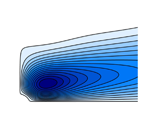
In contrast to the relatively simple structure of the density field, which is dominated by the first mode ( $\sin \theta$), the streamfunction field shown in figure 4 shows a richer spatial structure. The top row shows the far field whereas the bottom panel shows a small region near the cylinder. As the streamfunction field decays rapidly in the far field, to highlight the contours away from the cylinder, we plotted $\vert \psi \vert ^{1/4}$ in the figure. As can be gleaned from the figure, higher modes, $\sin m \theta$ with $m>1$ play a key role in tilting the streamlines to the right, away from the cylinder. In addition, the lower $\epsilon$ streamfunction shown in figure 4(b) occupies a larger fraction of spatial region, when compared with the higher $\epsilon$ flow shown in figure 4(a).

Figure 4. Spatial structure of  $\vert \psi \vert ^{1/4}$ for (a,c) $\epsilon =1$ and (b,d) $\epsilon =0.1$. In the top row, observe that the domain size is 10 times larger for the $\epsilon =0.1$ case when compared with the $\epsilon =1$ case. The bottom panels show the near-field structure by zooming in near the cylinder.
Figures 5–7 show the horizontal velocity ( $u$), vertical velocity ( $v$) and the magnitude of total velocity ( $\sqrt {u^2 + v^2}$) for two different $\epsilon$. The top row of these figures shows the far-field velocity whereas the bottom row highlights the near-field velocity, similar to the depiction in figure 4. On examining the horizontal velocity field shown in figure 5, we find that largest velocity values are negative and along the $x$-axis or $\theta =0$ direction. Therefore, the fluid is being dragged towards the cylinder along the $\theta =0$ direction. Along the same lines, examining the vertical velocity field in figure 6, it is seen that the velocity has largest magnitude along the $y$-axis or $\theta ={\rm \pi} /2$ direction, with the largest vertical velocity values being positive. The fluid is therefore being pushed away from the cylinder along the $\theta ={\rm \pi} /2$ direction. This velocity field, with the fluid being pulled in along $\theta =0$ direction and being pushed away along the $\theta ={\rm \pi} /2$ direction creates the recirculating flow around the cylinder, with closed streamlines shown in figure 4. As horizontal velocity achieves the largest values along $\theta =0$ direction and the vertical velocity attains the largest values along $\theta ={\rm \pi} /2$ direction, the net velocity magnitude shown in the last row of figure 7 shows two dominant values, along $\theta =0$ and $\theta ={\rm \pi} /2$ directions.

Figure 5. Spatial structure of  $u$ for (a,c) $\epsilon =1$ and (b,d) $\epsilon =0.1$. In the top row, observe that the domain size is 10 times larger for the $\epsilon =0.1$ case when compared with the $\epsilon =1$ case. The bottom panels show the near-field structure by zooming in near the cylinder.

Figure 6. Spatial structure of  $v$ for (a,c) $\epsilon =1$ and (b,d) $\epsilon =0.1$. In the top row, observe that the domain size is 10 times larger for the $\epsilon =0.1$ case when compared with the $\epsilon =1$ case. The bottom panels show the near-field structure by zooming in near the cylinder.

Figure 7. Spatial structure of  $\sqrt {u^2 + v^2}$ for (a,c) $\epsilon =1$ and (b,d) $\epsilon =0.1$. In the top row, observe that the domain size is 10 times larger for the $\epsilon =0.1$ case when compared with the $\epsilon =1$ case. The bottom panels show the near-field structure by zooming in near the cylinder.
Comparing the left and right columns of Figures 5–7 indicates the changes in the velocity field with changing  $\epsilon$. Similar to that seen in figure 4, the lower $\epsilon$ flow occupies a larger domain. In addition, as can be seen by comparing the magnitudes of the velocity in the left and right columns of Figures 5–7, the flow velocity decreases with decreasing $\epsilon$. Therefore, decreasing $\epsilon$ dilutes the flow: the flow occupies a larger region of space with reduced velocity magnitudes, with the flow eventually vanishing as $\epsilon \rightarrow 0$. This behaviour is the key difference between flow fields obtained at different $\epsilon$, apart from minor details in the spatial pattern of the flow fields at different $\epsilon$ seen in Figures 5–7.
3.2. Range of validity of the linear solution
Although the analytical solution of the linearised equation was derived assuming  $\epsilon \ll 1$, it is unclear at what $\epsilon$ the linear solution breaks down. To explore this we compared the solution of the linear equations (2.11) with the solution of the nonlinear equations (2.6) for different $\epsilon$. The numerical integrations were performed using the finite-element package COMSOL using a large square domain. We used triangular meshing elements with clustering of elements near the cylinder boundary. The grid was therefore extremely fine near the cylinder and gradually transitioned outwards at a pre-specified element growth rate. To mimic an unbounded domain, the domain was made significantly large such that the length of the domain was two orders of magnitude larger than the cylinder radius. The mesh and solver details are similar to that described in Camassa et al. (Reference Camassa, Harris, Hunt, Kilic and McLaughlin2019), especially see supplementary figure 1 and related description there.
The boundary conditions on the cylinder (2.7a) were directly imposed, whereas free-slip boundary conditions for velocity and Dirichlet boundary conditions for the density field were imposed on the far-field walls, to obtain the behaviour imposed by (2.7b). With a fixed domain, the mesh size was decreased until the solution was seen to be the same for three significant digits. Once a converged solution was obtained, the domain size was increased by a factor of 1.5 to check whether the solutions changed on increasing the domain size. The solution was considered converged if the solution was the same up to three significant digits with the larger domain size. To obtain numerically converged solutions for  $\epsilon \in [0.1, 5]$ that are discussed in the following, we found that a domain size of about 300 times the radius of the cylinder, with the finite-element size near the cylinder boundary being 0.015 times the radius of the cylinder, and an element growth of 1.012 was required in COMSOL.
To test the finite-element solver, we first integrated the linear equations (2.11) and compared the solutions so obtained with the analytical solution discussed earlier. By implementing the numerical procedure mentioned in the previous paragraph, it was seen that the relative error between the numerically converged solution of the linear equations and the analytical solution of the linear equations was insignificantly small. We then used the finite-element solver to solve the nonlinear equations (2.6) for a wide range of  $\epsilon$.
On comparing the linear and nonlinear solutions, we found that the linear solution agrees with the nonlinear solution for  $\epsilon \ll 1$ and even when $\epsilon \approx 1$. For an illustration, figure 8(a) shows the absolute value of the pointwise error between the velocity magnitude of the linear solution given in figure 7(a) and the corresponding nonlinear solution for $\epsilon =1$. On comparing figures 8(a) and 7(a), it is seen that the maximum pointwise error in the domain is an order of magnitude lower than the largest velocity magnitude of the linear solution. To quantify the difference between the linear and nonlinear solutions at different $\epsilon$, figure 8(b) shows the absolute value of the maximum pointwise difference between the linear and the nonlinear velocity magnitude, normalised by the maximum velocity magnitude from the nonlinear solution. Note that the error remains small at low $\epsilon$, although it grows with increasing $\epsilon$. The error remains small even when $\epsilon \approx 1$, although it becomes significant as $\epsilon$ exceeds 3. Therefore, although our analytical solution for the linear equations was derived for $\epsilon \ll 1$ regime, it can safely be used for flows that belong to the regime $\epsilon \lesssim 1$.

Figure 8. (a) Absolute value of the difference between the velocity magnitude of the linear solution and nonlinear solution for  $\epsilon =1$. (b) Maximum pointwise difference between the linear and nonlinear solution normalised by the maximum of velocity magnitude of the nonlinear solution. The inset shows a magnified version of the plot for $\epsilon$ in the interval $[0.1, 1]$.
We close this section by pointing out that the behaviour shown in figure 8 was generic for all fields, i.e. streamfunction, different velocity components, density and pressure, that we compared for different  $\epsilon$. We presented the velocity magnitude in figure 8 because this field showed the relatively largest difference between linear and nonlinear solutions, with other fields’ differences being relatively lesser in magnitude. Overall, the analytical solution agrees very well with the fully nonlinear solution up to $\epsilon \sim O(1)$ values, after which the two solutions start diverging.
4. Far-field decay rates of the flow
In the previous section we used the analytical solution (3.17a) and (3.18) to get the detailed flow structure of the self-induced flow generated by a cylinder. Although this provided detailed information on the density and flow fields at finite distances from the cylinder, it is still unclear how the solution behaves in the far field, other than the physical requirement that it vanish at infinity. Determining how rapid the solution decays away from the cylinder is important because this is the factor that decides the range of influence of the cylinder's flow field on other objects in its surroundings. However, the far-field behaviour cannot be deduced immediately from the exact expressions (3.17a) and (3.18), given their fairly complicated structure and the dependence on multiple special functions. An asymptotic analysis is needed to reveal the far-field behaviour by reducing these expressions to readily understandable simple functions; this is the focus of the present section, in which we concentrate on the flow component(s) of the solution, the density asymptotics following by a similar analysis.
As detailed in Appendix D, by using Taylor series expansions and Hankel transform techniques, we obtain the far-field decay estimates of the functions that appear in the streamfunction equation (3.18a) as
 $$\begin{gather} F_1^{(m)}(r) \sim \frac{ f_1(m) }{r_\epsilon^2} + \frac{ f_2(m) }{r_\epsilon^4} + O \left( \frac{1}{ r_\epsilon^6 } \right), \end{gather}$$
 $$\begin{gather}A_1^{(m,n)} \sim \frac{a_1 (m,n)}{r_\epsilon^{2n+2}} + O \left( \frac{1}{ r_\epsilon^{2n+4} } \right), \end{gather}$$
 $$\begin{gather}A_2^{(m,n)} \sim \frac{a_2 (m,n)}{r_\epsilon^{2n+2}} + O \left( \frac{1}{ r_\epsilon^{2n+4} } \right) , \end{gather}$$
 $$\begin{gather}A_3^{(m,n)} \sim \frac{a_3 (m,n)}{r_\epsilon^{2n}} + \frac{a_4 (m,n, \epsilon)}{r_\epsilon^{2n+2}} + O \left( \frac{1}{ r_\epsilon^{2n+4} } \right) , \end{gather}$$
where  $r_\epsilon = \epsilon r$ and the coefficients in (4.1) are given by
 $$\begin{gather} f_1 (m) =-2 \epsilon m, \end{gather}$$
 $$\begin{gather}f_2(m) = \epsilon (16 m^4 + \epsilon^2 m^3 -16 m^2 - \epsilon^2 m), \end{gather}$$
 $$\begin{gather}a_1 (m,n) = \frac{8n\epsilon^{2n-2}}{(2n)!} \frac{\varGamma(m+n+1)}{\varGamma(m-n)}, \end{gather}$$
 $$\begin{gather}a_2 (m,n) =-\frac{16n\epsilon^{2n-2}}{(2n-1)!} \frac{\varGamma(m+n+1)}{\varGamma(m-n)} , \end{gather}$$
 $$\begin{gather}a_3 (m,n) =-\frac{2(2n-1)\epsilon^{2n-1}}{(2n-2)!} \frac{\varGamma(m+n)}{\varGamma(m-n+1)} , \end{gather}$$
 $$\begin{gather}a_4 (m,n) =- 8(2n-1)\epsilon^{2n-1} \left \{ \frac{\epsilon^2}{4} \left( \frac{1}{ (2n)! } - \frac{1}{(2n-1)!} \right) - \frac{2m}{ (2n-2)! } \right\} \frac{\varGamma(m+n+1)}{\varGamma(m-n)}. \end{gather}$$
 From (4.1), we infer that all the functions appearing in the streamfunction equation (3.18a) decay algebraically for  $r \gg 1$. In addition, note that for a fixed order $m$, the $A$-functions decay faster with increasing $n$. The slowest decaying terms in (4.1) are $1/r_\epsilon ^2$ and $1/r_\epsilon ^4$, these corresponding to $n=1$ and $n=2$ in the $A$-functions.
Substituting (4.1) in (3.18a) and retaining terms up to  $1/ r_\epsilon ^4$ yields
 \begin{align} \psi^{(m)} (r) &\sim \frac{ a_1 (m,1) \tilde \omega_r^{(1)} }{ r_\epsilon^4 } + \frac{ a_2 (m,1) \tilde \omega^{(1)} }{ r_\epsilon^4 } + \frac{ a_3 (m,1) \tilde \rho^{(1)} }{ r_\epsilon^2 } + \frac{ a_4 (m,1) \tilde \rho^{(1)} }{ r_\epsilon^4 } , \nonumber\\ &\quad + \frac{ a_3 (m,2) \tilde \rho^{(2)} }{ r_\epsilon^4 } + \frac{ f_1 (m) }{ r_\epsilon^2 } + \frac{ f_2 (m) }{ r_\epsilon^4 } , \end{align}
 \begin{align} & =- 2 \epsilon m ( 1 +\tilde \rho^{(1)} ) \frac{ 1 }{ r_\epsilon^2 } , \\ &\quad + \{ 4(m^3 - m) ( \tilde \omega_r^{(1)} - 4 \tilde \omega^{(1)} ) + \epsilon ( 16m^4 + \epsilon^2 m^3 - 16 m^2 - \epsilon^2\,{m} ) ( 1 +\tilde \rho^{(1)} ) \} \frac{ 1 }{r_\epsilon^4 } . \nonumber \end{align}
We now take advantage of a series of infinite sums involving moments of cosine and sine functions (see chapter 1 of Gelfand & Shilov (Reference Gelfand and Shilov1964) for details):
 $$\begin{gather} \sum_{m=1}^{\infty} m \sin ( 2\,{m} \theta ) =- {\rm \pi}\sum_{ p=-\infty }^{ \infty } \delta' (2 \theta - 2 p {\rm \pi}) , \end{gather}$$
 $$\begin{gather}\sum_{m=1}^{\infty} m^2 \sin ( 2\,{m} \theta ) = \frac{1}{4} \frac{\cos \theta }{ \sin^3 \theta }, \end{gather}$$
 $$\begin{gather}\sum_{m=1}^{\infty} m^3 \sin ( 2\,{m} \theta ) = \frac{ {\rm \pi}}{ 4 } \sum_{ p=-\infty }^{ \infty } \delta''' (2 \theta - 2 p {\rm \pi}) , \end{gather}$$
 $$\begin{gather}\sum_{m=1}^{\infty} m^4 \sin ( 2\,{m} \theta ) =-\frac{1}{4} \frac{\cos \theta (2 + \cos^2 \theta) }{ \sin^5 \theta }. \end{gather}$$
In these expressions,  $\delta (\theta )$ refers to the Dirac delta function and the primes denote its derivatives, e.g. $\delta ' (\theta )$ and $\delta '' (\theta )$ denote the first and second derivatives of $\delta (\theta )$, defined in the sense of generalised functions (Gelfand & Shilov Reference Gelfand and Shilov1964).
Substituting (4.3a) into the streamfunction equation given in (3.17a) and performing the sum using the expressions in (4.4) gives
 \begin{equation} \psi \sim- 12 \epsilon ( 1 +\tilde \rho^{(1)}) \left( \frac{ \cos \theta }{ \sin^5 \theta } \right) \frac{ 1 }{ r_\epsilon^4 }. \end{equation}
To arrive at this expression we ignored terms such as  $\delta ' (2 \theta - 2 p {\rm \pi})$ and $\delta ''' (2 \theta - 2 p {\rm \pi})$ after performing the summation over $m$, because the support of these terms is on the rays $\theta =p {\rm \pi}$. In addition, the streamfunction expansion in terms of $\sin (2m \theta )$ in (3.17a) guarantees that $\psi =0$ on the rays $\theta =p {\rm \pi}$. Therefore, (4.5) is the generic far-field decay rate of the streamfunction, valid along rays with fixed $\theta$. As $r_\epsilon = \epsilon r$, the expression in (4.5) indicates that for a fixed $\epsilon$, the streamfunction decays algebraically in the far field along rays with fixed $\theta$, as $1/r^4$. In addition, the appearance of $\cos \theta$ and $\sin \theta$ in (4.5) indicates that the decay in streamfunction can depend on the direction along which the limit $r \to \infty$ is taken, as can be inferred from figure 4. In figure 9, the streamfunction based on the analytical solution for $\epsilon =1$ is plotted corresponding to $\theta = {\rm \pi}/\sqrt {10}$, an arbitrary direction where the irrational number $\sqrt {10}$ ensures that $\sin (m \theta )$ in the summation over $m$ in (3.17a) is, in general, non-zero for any $m$. From the red curve in figure 9, showing logarithm of the absolute value of the streamfunction field vs $\log \ r$, it is seen that the streamfunction is a straight line with slope $-4$, indicative of the $1/r^4$ decay predicted by (4.5).

Figure 9. Absolute value of the streamfunction, horizontal velocity along  $\theta =0$ and vertical velocity along $\theta ={\rm \pi} /2$ direction on a log–log scale. The radial value $r=50$ is the starting point of the $x$-axis, so as to exclude the near-field region around the cylinder. All curves are straight lines, reflecting the algebraic decay of the flow with distance away from the cylinder.
We now examine the decay rate of velocity in the far field. For this, we first examine the radial velocity field,  $v_r$, as
 \begin{equation} v_r = \frac{1}{r} \frac{\partial{ \psi }}{\partial{ \theta }} = \sum_{m=1}^{\infty} 2m \psi^{(m)} (r) \cos ( 2m \theta ). \end{equation}
To simplify further, we substitute (4.3a) in (4.6) and use relationships similar to those in (4.4) (see chapter 1 of Gelfand & Shilov Reference Gelfand and Shilov1964):
 $$\begin{gather} \sum_{m=1}^{\infty} m^2 \cos ( 2\,{m} \theta ) =- {\rm \pi}\sum_{ p=-\infty }^{ \infty } \delta'' (2 \theta - 2 p {\rm \pi}) , \end{gather}$$
 $$\begin{gather}\sum_{m=1}^{\infty} m^3 \cos ( 2\,{m} \theta ) =- \frac{ 1 + 2 \cos^2 \theta }{ 8 \sin^4 \theta }, \end{gather}$$
 $$\begin{gather}\sum_{m=1}^{\infty} m^4 \cos ( 2\,{m} \theta ) = {\rm \pi}\sum_{ p=-\infty }^{ \infty } \delta'''' (2 \theta - 2 p {\rm \pi}) , \end{gather}$$
 $$\begin{gather}\sum_{m=1}^{\infty} m^5 \cos ( 2\,{m} \theta ) =-\frac{1}{8} \frac{ 2 \cos^4 \theta + 11 \cos^2 \theta + 2 }{ \sin^6 \theta }. \end{gather}$$
We thus obtain
 \begin{equation} v_r \sim-4 \epsilon^2 ( 1 +\tilde \rho^{(1)}) \left( \frac{ 4 \cos^4 \theta + 10 \cos^2 \theta + 1 }{ \sin^6 \theta } \right) \frac{1}{ r_\epsilon^5 } . \end{equation}
Note that this expression for radial velocity does not apply for the  $\theta =0$ direction. In addition, unlike the streamfunction which vanishes along the $\theta =0$ direction, radial velocity is non-zero on the $\theta =0$ ray, indicating that this asymptotic formula breaks down for this value of $\theta$. The breakdown of the asymptotic formula is inevitable also if the limit $r \to \infty$ is taken along horizontal directions whereby $y$ is kept constant while $x\to \infty$. We therefore conclude from (4.8) that the radial velocity along rays with fixed $\theta \neq 0$ decays as $1/r^5$.
Similar to the procedure for obtaining radial velocity, we can obtain the tangential velocity  $v_\theta = - \partial \psi /\partial r$. As can be checked, we obtain the same final expression for the tangential velocity by differentiating the far-field expression for streamfunction in (4.3a) and performing the summations. This strategy works because the expressions in (4.3a) do not diverge on differentiating with respect to $r$, despite the series being asymptotic in $r$. The final result of the calculation is that the tangential velocity also decays as $1/r^5$, away from the $\theta =0$ direction. In addition, the tangential velocity is zero on the $\theta =0$ and the $\theta ={\rm \pi} /2$ rays. Therefore, the tangential velocity decays as $1/r^5$ in general. As both radial and tangential velocity decays as $1/r^5$, the total velocity magnitude also decays as $1/r^5$, away from the $\theta =0$ direction. The black curve in figure 9 shows the vertical velocity $v$ along the $\theta ={\rm \pi} /2$ direction, which corresponds to the total velocity magnitude and also the radial velocity along the same direction. The curve appears as a straight line with slope $-5$ on the log–log axes, indicating the $1/r^5$ decay rate predicted previously.
As mentioned before, although the tangential velocity is zero along  $\theta =0$, the radial velocity is non-zero on this ray and the far-field decay rate predicted by (4.8) does not apply in this special direction (and, in fact, for any horizontal direction which would approach the value $\theta =0$ as $r\to \infty$). This is reflected by the generalised function approach involving infinite sums we used earlier which would generate singularities with $\theta =0$. Therefore, we need to implement a completely new procedure to find the velocity decay rate along $\theta =0$ directions. For this, we first set $\theta =0$ in (4.6) to get
 \begin{align} v_r (\theta=0) &= \frac{1}{r} \sum_{m=1}^{\infty} 2m \psi^{(m)} (r) , \end{align}
 \begin{align} & = \frac{1}{r} \sum_{m=1}^{\infty} 2m \left \{ \sum_{n=1}^{\infty} \left( A_1^{(m,n)} \tilde \omega_r^{(n)} + A_2^{(m,n)} \tilde \omega^{(n)} + A_3^{(m,n)} \tilde \rho^{(n)} \right) + F_1^{(m)} \right \}. \end{align}
To perform these summations, we now replace the  $r$-dependent functions, $A_1^{(m,n)}$, $A_2^{(m,n)}$, $A_3^{(m,n)}$ and $F_1^{(m)}$, with a set of functions that asymptotically approximates them. Specifically, in Appendix E, we show that the functions that appear in (4.9b) have the following leading-order asymptotics:
 $$\begin{gather} F_1^{(m)}(r) \sim- \frac{2m \epsilon}{r_\epsilon^2} \,{\rm e}^{-8m^3/r_\epsilon^2}, \end{gather}$$
 $$\begin{gather}A_1^{(m,1)}(r) \sim \frac{4m^4 \epsilon}{r_\epsilon^4}\, {\rm e}^{-8m^3/r_\epsilon^2} , \end{gather}$$
 $$\begin{gather}A_2^{(m,1)}(r) \sim- \frac{24m^4 \epsilon}{r_\epsilon^4}\, {\rm e}^{-8m^3/r_\epsilon^2} , \end{gather}$$
 $$\begin{gather}A_3^{(m,1)}(r) \sim- \frac{2m \epsilon}{r_\epsilon^2}\, {\rm e}^{-8m^3/r_\epsilon^2} . \end{gather}$$
In general, the coefficients  $A^{(m,n)}$ for $n>1$ decay faster than the functions above and are therefore discarded in the summation. Furthermore, as described in detail in Appendix E, the asymptotics of functions in (4.10) is derived assuming $r \gg 1$ and $m \gg 1$. For an illustration, figure 10 compares $F_1^{(m)}(r)$ computed exactly with its asymptotic expression $- ({2m \epsilon }/{r_\epsilon ^2})\, {\rm e}^{-8m^3/r_\epsilon ^2}$ for different $m$. Although the asymptotic approximation was derived assuming high $m$ and $r \gg 1$, the approximation is seen to work really well even for $m=1$ for $r \gg 1$.

Figure 10. Plots of  $F_1^{(m)}(r)$ for $\epsilon =1$ and $m=1$, 2 and 3. The black, blue and red curves are the same curves that appear in figure 2(a). The thin green curves are the approximations $F_1^{(m)} \sim - ({2m \epsilon }/{r_\epsilon ^2})\, {\rm e}^{-8m^3/r_\epsilon ^2}$. The inset in the figure shows the comparison for $r \gg 1$.
We now use the asymptotic expressions in (4.10) to compute the sum in (4.9b). Using the expression in (4.10a), we obtain
 \begin{equation} \sum_{m=1}^{\infty} 2m F_1^{(m)} =- 4 \frac{\epsilon^2}{ r_\epsilon^3 } \sum_{m=1}^{\infty} m^2 \,{\rm e}^{-8m^3/r_\epsilon^2} \sim- 4 \frac{\epsilon^2}{ r_\epsilon^3 } \int_{0}^{\infty} m^2 \,{\rm e}^{-8m^3/r_\epsilon^2} \,{\rm d} m =- \frac{ \epsilon^2 }{ r_\epsilon} . \end{equation}
With a similar reasoning, we obtain  $\sum _{m=1}^{\infty } 2m A_3^{(m, 1)} = - \epsilon ^2/ r_\epsilon$. The other $A$ functions that appear in (4.9b) contribute terms that decay faster with distance. For instance, using the expressions in (4.10), we obtain $\sum _{m=1}^{\infty } 2m A_1^{(m, 1)} \sim \sum _{m=1}^{\infty } 2m A_2^{(m, 1)} \sim O(1/ r_\epsilon ^{5/3})$. Therefore, we have
 \begin{equation} v_r (\theta=0) \sim- \epsilon^2 ( 1 +\tilde \rho^{(1)} ) \frac{ 1 }{ r_\epsilon } , \end{equation}
implying that the velocity magnitude in the equatorial plane decays as  $1/r$. The blue curve in figure 9 shows the horizontal velocity $u$ along the $\theta =0$ direction for $\epsilon =1$, which corresponds to the total velocity magnitude and radial velocity along the same direction. The curve appears as a straight line with slope $-1$, confirming the $1/r$ decay rate prediction from the asymptotic estimate in (4.12). Therefore velocity in the far field decays slowest along the $\theta =0$ direction, this being the direction that is least affected by density stratification.
We conclude this section by pointing out one final feature of the self-induced flow around the cylinder, specifically a feature of the recirculating flow cells that emerge in the flow induced by the cylinder. Taking advantage of the far-field asymptotics carried out on (4.9) with the dependence on the angle  $\theta$ maintained, it can be shown that beyond a certain separating streamline extending to infinity, whose location depends on $\epsilon$, the approach to zero of the vertical component of the velocity along a vertical straight line at fixed $x$ is monotonic. Below such streamline the vertical velocity component alternates sign exactly three times, thus showing that the total number of recirculating bands in each quadrant is just four, with the last one extending to infinity along the vertical direction. This analysis therefore points out that the flow structure of recirculation bands seen in our velocity plots consists of only a finite number of such bands. Of course, in practical situations, such as in laboratory experiments, container boundaries could affect the weak far-field flow. Consequently, this result about the existence of only a finite number of recirculation bands in the cylinder-induced flow would be challenging to verify experimentally and might be primarily of theoretical interest especially in view of the idealization of constant density stratifications in infinite domains, which would eventually lead to zero density for increasing height.
5. Summary and discussion
In this paper we have examined the self-induced flow generated by an infinitely long cylinder at rest in a stratified fluid. In the low Péclet limit we used a Green's function approach to find analytical solution for the flow field over a cylinder. The analytical solution is given in terms of multiple special functions and is challenging to interpret in terms of simple functions. We therefore deduced properties of the functions and their features to infer qualitative details of the flow field. Furthermore, we used asymptotic expansions of the analytic solution to determine the far-field behaviour of the flow field, and specifically the decay rate of the flow away from the cylinder.
On comparing the analytical solution quantitatively with the numerical solution of the nonlinear equations, we found that the analytical solution agrees with the nonlinear solution even for Péclet numbers approaching unity. On moving from asymptotically small to  $O(1)$ Péclet numbers, the flow was seen to become stronger in smaller spatial regions concentrated near the cylinder.
As pointed out by List (Reference List1971), Ardekani & Stocker (Reference Ardekani and Stocker2010) and Fouxon & Leshansky (Reference Fouxon and Leshansky2014) using solutions of the linearised equations forced with Dirac delta functions (and, thus, different from a boundary value problem), Stokes flow in a stratified fluid is significantly different from its homogeneous counterpart, the latter being generated in the absence of stratification. Although homogeneous Stokes flow consists of open streamlines, closed streamlines with recirculation zones are a characteristic feature of Stokes flow in a stratified fluid, as can be seen in figures 4–7. Our asymptotic analysis of the flow revealed that the streamfunction decays as  $1/r^4$, which leads to velocity that decays as $1/r^5$ in the far field. Furthermore, the decay rate is different along directions parallel to the ‘equatorial’ plane $\theta =0$, where the velocity decays as $1/r$ in the far field. Therefore, the velocity decays slowest in horizontal directions normal to gravity, where the effects of stratification is least felt.
Intriguingly, as mentioned previously, the self-induced flow over a cylinder decays algebraically in the far field and this may be compared with other known decay estimates. As shown by Phillips (Reference Phillips1970) and Wunsch (Reference Wunsch1970), self-induced flow over an inclined flat plate in a stratified fluid decays exponentially in the far field. Therefore on moving from one to two dimensions, the decay rate of the flow is slower for self-induced flow. In other words, the flow decays faster in one dimension. It might be useful to compare the decay rate of the flow we obtained with that of homogeneous Stokes flow over a cylinder. We recall that the Stokes flow over a slow moving cylinder decays exponentially in the far field (Stokes Reference Stokes1851; Oseen Reference Oseen1910; Lamb Reference Lamb1911; Van Dyke Reference Van Dyke1975). Of course, it is important to keep in mind the differences between these set-ups, because there is no concept of self-induced flow in a homogeneous fluid, nor it is necessary for an object to move in order to generate flow in the stratified case, although in both set-ups the Reynolds number of the flow is assumed to be (asymptotically) small. Nevertheless, it is interesting to compare decay rates and point out that the self-induced one in a stratified fluid is algebraic and therefore much slower than the exponential rate of the flow by a moving cylinder in homogeneous Stokes flow. Thus, we stress that the far-field algebraic decay rates we obtained are not necessarily anticipated on purely physical grounds, and in particular that their exact nature, such as the  $1/r^4$ power law for the stream function along non-horizontal rays, was provided by analysis of an exact, albeit fairly complicated, solution of an elliptic boundary value problem. Such asymptotic results for functional behaviour in the far-field limit could then be useful for modelling the body as a point object with the far-field structure prescribed, which, in turn, could be used to greatly simplify simulations of the time evolution of interacting bodies, as long as sufficiently large distances from each other are maintained.
An inspiration for the present work was, in fact, provided by the clustering of particles in a stratified fluid, in the absence of adhesive forces, reported in Camassa et al. (Reference Camassa, Harris, Hunt, Kilic and McLaughlin2019). The interaction of bodies due to the self-induced flows and the resulting clustering would be more efficient if the flow decayed slowly in the far field. In this regard, the finding in this work of an algebraic decay rate for flow being slower than exponential decay of homogeneous Stokes flow implies that the interaction of multiple bodies in two dimensions could be stronger under the influence of self-induced flow when compared with the hydrodynamics interactions under homogeneous Stokes flow. Based on our findings, we speculate that the interaction of elongated rod-like structures could be dominated by the influence of the self-induced flow generated in a stratified fluid.
Related to the discussion of bodies interacting via self-induced flows, we note that the Green's function procedure we used to compute the flow over a cylinder can be applied to bodies of arbitrary shape. Equations similar to (3.14) can be developed for arbitrary shapes, although further simplification to obtain analytical solution such as those we obtained in this paper might not be straightforward for arbitrary shapes. Nevertheless, boundary integral equations such as (3.14) can be solved for arbitrary bodies numerically, resulting in self-induced flows over arbitrary bodies. As can be seen in the work of Drescher et al. (Reference Drescher, Goldstein, Michel, Polin and Tuval2010), the geometry of the body plays a key role in setting the flow and the resulting flow field can deviate from the singularity solutions developed in List (Reference List1971), Ardekani & Stocker (Reference Ardekani and Stocker2010) and Fouxon & Leshansky (Reference Fouxon and Leshansky2014) which fail to capture the self-induced nature of our flows. In contrast, the boundary integral formalism leading to equations such as (3.14) can be applied to arbitrary bodies and can be used to obtain accurate solutions for self-induced flows over arbitrary bodies. Future work could pursue this route to obtain flows over arbitrary shaped bodies.
Finally, we recall that the analytical approach we used was formally for low Péclet regime ( $\epsilon \ll 1$), although the solution was seen to match direct numerical computations of the full Navier–Stokes equations up to $\epsilon \approx 1$. Nevertheless, as seen from figure 8(b), the linear solution departs from the nonlinear solution for $\epsilon \gg 1$. Based on the results presented in this work and our extensive numerical integration of the nonlinear equations, self-induced flows generally become stronger at higher Péclet numbers, a feature which would assist in the interaction and clustering of objects. A careful study of self-induced flows at asymptotically large Péclet numbers remains unexplored territory. Similar to the problem of homogeneous Stokes flow over a cylinder, matched asymptotic techniques could be used to examine the self-induced flow over a cylinder at high Péclet number. The properties of the flow at asymptotically high Péclet numbers, specifically the far-field decay rates of the flow at high Péclet numbers in comparison with the low Péclet results we presented here would make an exciting future follow-up study to the present work.
Acknowledgements
The authors are grateful for multiple insightful discussions with and helpful comments from Rich McLaughlin and Robert Hunt.
Funding
J.T. acknowledges support from the Science and Engineering Research Board (SERB) of India through the project SRG/2022/001071. R.C. is grateful for the support provided by the National Science Foundation under grants RTG DMS-0943851, CMG ARC-1025523, DMS-1009750, DMS-1517879 and DMS-1910824 and by the Office of Naval Research under grants N00014-18-1-2490 and DURIP N00014-12-1-0749.
Declaration of interests
The authors report no conflict of interest.
Appendix A
In this appendix we provide the intermediate steps required in obtaining formulae (3.18). Using the expressions in (3.17a), at  $r=1$ we have
 \begin{equation} \left. \begin{array}{c} \displaystyle \psi (r=1, \theta ) = \sum_{m=1}^{\infty} \tilde \psi^{(m)} \sin(2m \theta), \quad \rho(r=1, \theta) = \sum_{m=1}^{\infty} \tilde{\rho}^{(m)} \sin(2m-1) \theta, \\ \displaystyle \omega (r=1, \theta) = \sum_{m=1}^{\infty} \tilde{\omega}^{(m)} \sin2m \theta, \quad \omega_r (r=1, \theta) = \sum_{m=1}^{\infty} \tilde{\omega}_r^{(m)} \sin2m \theta, \end{array}\right\} \end{equation}
where we use tildes to denote variables at  $r=1$, such as $\tilde \omega ^{(m)} = \omega ^{(m)} (r=1)$ for example. Substituting (A1) into (3.14) and simplifying gives
 \begin{align} \psi(r, \theta) &=-
\frac{1}{4 {\rm \pi}}\sum_{m=1}^{\infty} (-1)^m \tilde
\omega_r^{(m)} \int_{0}^{\infty} \int_{0}^{2 {\rm \pi}} \frac{2
k J_{2m}(k) \sin(2m \theta_k) }{k^4 + \epsilon^4 \cos^2
\theta_k}\, {\rm e}^{-{\rm i} k r \cos(\theta_k - \theta)}
\, {\rm d} \theta_k \, {\rm d} k \nonumber\\ &\quad -
\frac{1}{4 {\rm \pi}}\sum_{m=1}^{\infty} (-1)^m \tilde
\omega^{(m)} \int_{0}^{\infty} \int_{0}^{2 {\rm \pi}} \frac{ k^2
[ J_{2m+1}(k) - J_{2m-1}(k) ] \sin(2m \theta_k) }{k^4 +
\epsilon^4 \cos^2 \theta_k}\notag\\ &\quad \times {\rm e}^{-{\rm i} k r
\cos(\theta_k - \theta)} \, {\rm d} \theta_k \, {\rm d} k \nonumber\\ &\quad + \frac{\epsilon^3}{4
{\rm \pi}}\sum_{m=1}^{\infty} (-1)^m \tilde \rho^{(m)}
\int_{0}^{\infty} \int_{0}^{2 {\rm \pi}}\notag\\ &\quad \times \left\{ \frac{ k [
J_{2m}(k) + J_{2m-2}(k) ] [ \sin ( 2m \theta_k ) - \sin (
(2m-2) \theta_k )]}{2 ( k^4 + \epsilon^4 \cos^2 \theta_k
)}\vphantom{\frac{\epsilon^3}{4 {\rm \pi}}}{\rm e}^{-{\rm i} k r
\cos(\theta_k - \theta)} \right\} \, {\rm d} \theta_k \,
{\rm d} k \nonumber\\ &\quad + \frac{\epsilon^3}{4 {\rm \pi}}
\int_{0}^{\infty} \int_{0}^{2 {\rm \pi}} \frac{ J_1(k) \sin(2
\theta_k) }{k^4 + \epsilon^4 \cos^2 \theta_k}\, {\rm
e}^{-{\rm i} k r \cos(\theta_k - \theta)} \, {\rm d}
\theta_k \, {\rm d} k,
\end{align}
\begin{align} \psi(r, \theta) &=-
\frac{1}{4 {\rm \pi}}\sum_{m=1}^{\infty} (-1)^m \tilde
\omega_r^{(m)} \int_{0}^{\infty} \int_{0}^{2 {\rm \pi}} \frac{2
k J_{2m}(k) \sin(2m \theta_k) }{k^4 + \epsilon^4 \cos^2
\theta_k}\, {\rm e}^{-{\rm i} k r \cos(\theta_k - \theta)}
\, {\rm d} \theta_k \, {\rm d} k \nonumber\\ &\quad -
\frac{1}{4 {\rm \pi}}\sum_{m=1}^{\infty} (-1)^m \tilde
\omega^{(m)} \int_{0}^{\infty} \int_{0}^{2 {\rm \pi}} \frac{ k^2
[ J_{2m+1}(k) - J_{2m-1}(k) ] \sin(2m \theta_k) }{k^4 +
\epsilon^4 \cos^2 \theta_k}\notag\\ &\quad \times {\rm e}^{-{\rm i} k r
\cos(\theta_k - \theta)} \, {\rm d} \theta_k \, {\rm d} k \nonumber\\ &\quad + \frac{\epsilon^3}{4
{\rm \pi}}\sum_{m=1}^{\infty} (-1)^m \tilde \rho^{(m)}
\int_{0}^{\infty} \int_{0}^{2 {\rm \pi}}\notag\\ &\quad \times \left\{ \frac{ k [
J_{2m}(k) + J_{2m-2}(k) ] [ \sin ( 2m \theta_k ) - \sin (
(2m-2) \theta_k )]}{2 ( k^4 + \epsilon^4 \cos^2 \theta_k
)}\vphantom{\frac{\epsilon^3}{4 {\rm \pi}}}{\rm e}^{-{\rm i} k r
\cos(\theta_k - \theta)} \right\} \, {\rm d} \theta_k \,
{\rm d} k \nonumber\\ &\quad + \frac{\epsilon^3}{4 {\rm \pi}}
\int_{0}^{\infty} \int_{0}^{2 {\rm \pi}} \frac{ J_1(k) \sin(2
\theta_k) }{k^4 + \epsilon^4 \cos^2 \theta_k}\, {\rm
e}^{-{\rm i} k r \cos(\theta_k - \theta)} \, {\rm d}
\theta_k \, {\rm d} k,
\end{align} \begin{align} \rho(r,
\theta) &=- \frac{{\rm i} \epsilon }{4 {\rm \pi}}\sum_{m=1}^{\infty} (-1)^m \tilde \omega_r^{(m)}
\int_{0}^{\infty} \int_{0}^{2 {\rm \pi}} \left\{ \frac{
J_{2m}(k) ( \sin( (2m +1) \theta_k) + \sin( (2m -1)
\theta_k) ) }{k^4 + \epsilon^4 \cos^2 \theta_k} \right. \nonumber\\
&\quad \times \left. {\rm e}^{-{\rm i} k r \cos(\theta_k - \theta)}
\vphantom{\frac{\epsilon^3}{4 {\rm \pi}}}\right\} \, {\rm d} \theta_k \, {\rm d} k \nonumber\\
&\quad - \frac{ {\rm i} \epsilon }{4
{\rm \pi}}\sum_{m=1}^{\infty} (-1)^m \tilde \omega^{(m)}
\int_{0}^{\infty} \int_{0}^{2 {\rm \pi}} \left\{ {\rm e}^{-{\rm
i} k r \cos(\theta_k - \theta)}
\vphantom{\frac{\epsilon^3}{4 {\rm \pi}}}\right. \nonumber\\
&\quad \times \left. \frac{ k [ J_{2m+1}(k) - J_{2m-1}(k) ] ( \sin(
(2m +1) \theta_k) + \sin( (2m -1) \theta_k) ) }{ 2 ( k^4 +
\epsilon^4 \cos^2 \theta_k ) } \right\} \, {\rm d} \theta_k
\, {\rm d} k \nonumber\\ &\quad + \frac{i}{4
{\rm \pi}}\sum_{m=1}^{\infty} (-1)^m \tilde \rho^{(m)}
\int_{0}^{\infty} \int_{0}^{2 {\rm \pi}} \frac{ {\rm e}^{-{\rm
i} k r \cos(\theta_k - \theta)} }{k^4 + \epsilon^4 \cos^2
\theta_k} \left \{ \frac{\epsilon^4}{2} \sin ( (2m+1)
\theta_k ) J_{2m}(k) \right. \nonumber\\ &\quad \left. +
\sin ( ( 2m-1) \theta_k ) \left( k^4 + \frac{\epsilon^4}{2}
\right) [ J_{2m}(k) - J_{2m-2}(k) ] \right. \nonumber\\
&\quad - \left.\frac{\epsilon^4}{2} \sin ( (2m-3) \theta_k
) J_{2m-2}(k) \right\} \, {\rm d} \theta_k \, {\rm d} k
\nonumber\\ &\quad - \frac{i}{4 {\rm \pi}} \int_{0}^{\infty}
\int_{0}^{2 {\rm \pi}} \frac{ 2 k^3 J_1(k) \sin \theta_k }{k^4 +
\epsilon^4 \cos^2 \theta_k}\, {\rm e}^{-{\rm i} k r
\cos(\theta_k - \theta)} \, {\rm d} \theta_k \, {\rm d} k .
\end{align}
\begin{align} \rho(r,
\theta) &=- \frac{{\rm i} \epsilon }{4 {\rm \pi}}\sum_{m=1}^{\infty} (-1)^m \tilde \omega_r^{(m)}
\int_{0}^{\infty} \int_{0}^{2 {\rm \pi}} \left\{ \frac{
J_{2m}(k) ( \sin( (2m +1) \theta_k) + \sin( (2m -1)
\theta_k) ) }{k^4 + \epsilon^4 \cos^2 \theta_k} \right. \nonumber\\
&\quad \times \left. {\rm e}^{-{\rm i} k r \cos(\theta_k - \theta)}
\vphantom{\frac{\epsilon^3}{4 {\rm \pi}}}\right\} \, {\rm d} \theta_k \, {\rm d} k \nonumber\\
&\quad - \frac{ {\rm i} \epsilon }{4
{\rm \pi}}\sum_{m=1}^{\infty} (-1)^m \tilde \omega^{(m)}
\int_{0}^{\infty} \int_{0}^{2 {\rm \pi}} \left\{ {\rm e}^{-{\rm
i} k r \cos(\theta_k - \theta)}
\vphantom{\frac{\epsilon^3}{4 {\rm \pi}}}\right. \nonumber\\
&\quad \times \left. \frac{ k [ J_{2m+1}(k) - J_{2m-1}(k) ] ( \sin(
(2m +1) \theta_k) + \sin( (2m -1) \theta_k) ) }{ 2 ( k^4 +
\epsilon^4 \cos^2 \theta_k ) } \right\} \, {\rm d} \theta_k
\, {\rm d} k \nonumber\\ &\quad + \frac{i}{4
{\rm \pi}}\sum_{m=1}^{\infty} (-1)^m \tilde \rho^{(m)}
\int_{0}^{\infty} \int_{0}^{2 {\rm \pi}} \frac{ {\rm e}^{-{\rm
i} k r \cos(\theta_k - \theta)} }{k^4 + \epsilon^4 \cos^2
\theta_k} \left \{ \frac{\epsilon^4}{2} \sin ( (2m+1)
\theta_k ) J_{2m}(k) \right. \nonumber\\ &\quad \left. +
\sin ( ( 2m-1) \theta_k ) \left( k^4 + \frac{\epsilon^4}{2}
\right) [ J_{2m}(k) - J_{2m-2}(k) ] \right. \nonumber\\
&\quad - \left.\frac{\epsilon^4}{2} \sin ( (2m-3) \theta_k
) J_{2m-2}(k) \right\} \, {\rm d} \theta_k \, {\rm d} k
\nonumber\\ &\quad - \frac{i}{4 {\rm \pi}} \int_{0}^{\infty}
\int_{0}^{2 {\rm \pi}} \frac{ 2 k^3 J_1(k) \sin \theta_k }{k^4 +
\epsilon^4 \cos^2 \theta_k}\, {\rm e}^{-{\rm i} k r
\cos(\theta_k - \theta)} \, {\rm d} \theta_k \, {\rm d} k .
\end{align}
We then multiply (A2a) by  $\sin (2n \theta )$ and (A2b) by $\sin ((2n-1) \theta )$, use the expansion in (3.17a), and integrate from $\theta = 0$ to $2 {\rm \pi}$. This gives us
 $$\begin{gather} \psi^{(n)} (r) = \sum_{n=1}^{\infty} [ A_1^{(n,m)}(r) \tilde \omega_r^{(m)} + A_2^{(n,m)}(r) \tilde \omega^{(m)} + A_3^{(n,m)}(r) \tilde \rho^{(m)} ] + F_1^{(n)} (r) , \end{gather}$$
 $$\begin{gather}\rho^{(n)} (r) = \sum_{n=1}^{\infty} [ B_1^{(n,m)}(r) \tilde \omega_r^{(m)} + B_2^{(n,m)}(r) \tilde \omega^{(m)} + B_3^{(n,m)}(r) \tilde \rho^{(m)} ] + F_2^{(n)} (r) . \end{gather}$$
Appendix B
The functions that appear in (3.18) are given by
 \begin{equation} \left. \begin{array}{l}
\displaystyle A_1^{(m,n)}(r) = \int_{0}^{\infty} k J_{2m}(k
r) J_{2n}(k) \{ Q_{m-n} (k, \epsilon) - Q_{m+n} (k,
\epsilon) \} \, {\rm d} k,\\
\displaystyle A_2^{(m,n)}(r) = \int_{0}^{\infty} k^2
J_{2m}(k r) [ J_{2n + 1}(k) - J_{2n - 1}(k) ] \{ Q_{m-n}
(k, \epsilon) - Q_{m+n} (k, \epsilon) ] \, {\rm d} k,
\\ \begin{aligned} A_3^{(m,n)}(r) &
=-\dfrac{\epsilon^3}{4} \int_{0}^{\infty} k J_{2m}(k r) [
J_{2n}(k) + J_{2n - 2}(k) ]\{ Q_{m-n} (k, \epsilon) -
Q_{m+n} (k, \epsilon) \\ & \quad+
Q_{m-n+1} (k, \epsilon) - Q_{m+n-1} (k, \epsilon) \} \,
{\rm d} k, \end{aligned}\\ \displaystyle
F_1^{(m)} (r) =-\dfrac{\epsilon^3}{2 } \int_{0}^{\infty}
J_{2m}(k r) J_1 (k) \{ Q_{m-1} (k, \epsilon) - Q_{m+1} (k,
\epsilon) \} \, {\rm d} k ,\\
\begin{aligned} B_1^{(m,n)}(r) & =-\dfrac{\epsilon}{2}
\int_{0}^{\infty} J_{2m-1}(k r) J_{2n}(k) \{ Q_{m+n} (k,
\epsilon) - Q_{m+n-1} (k, \epsilon) - Q_{m-n} (k, \epsilon)
\\ & \quad + Q_{m-n-1} (k, \epsilon)
\}\, {\rm d} k ,\end{aligned}\\
\begin{aligned} B_2^{(m,n)}(r) & =-\dfrac{ \epsilon }{4 }
\int_{0}^{\infty} k J_{2m-1}(k r) [ J_{2n + 1}(k) - J_{2n -
1}(k) ] \{ Q_{m+n} (k, \epsilon) - Q_{m+n-1} (k,
\epsilon)\\ & \quad - Q_{m-n} (k,
\epsilon) + Q_{m-n-1} (k, \epsilon) \} \, {\rm d} k,
\end{aligned}\\ \begin{aligned}
B_3^{(m,n)}(r) & =-\dfrac{1}{2 } \int_{0}^{\infty}
J_{2m-1}(k r) \, {\rm d} k \left \{ - \dfrac{\epsilon^4}{2}
J_{2n}(k) [ Q_{m+n} (k_\epsilon) + Q_{m-n-1} (k_\epsilon) ]
\right.\\ & \quad + \left( k^4 +
\dfrac{\epsilon^4}{2} \right) [ J_{2n}(k) - J_{2n-2}(k) ][
Q_{m-n} (k, \epsilon) + Q_{m+n-1} (k, \epsilon) ] \\
& \quad + \left.
\dfrac{\epsilon^4}{2} J_{2n-2} (k) [ Q_{m+n-2} (k,
\epsilon) + Q_{m-n+1} (k, \epsilon)] \right\} \end{aligned},\\ F_2^{(m)} (r) =
\int_{0}^{\infty} k^3 J_{2m-1}(k r) J_1 (k) [ Q_{m-1} (k,
\epsilon) + Q_{m} (k, \epsilon) ] \, {\rm d} k,
\end{array}\right\}
\end{equation}
\begin{equation} \left. \begin{array}{l}
\displaystyle A_1^{(m,n)}(r) = \int_{0}^{\infty} k J_{2m}(k
r) J_{2n}(k) \{ Q_{m-n} (k, \epsilon) - Q_{m+n} (k,
\epsilon) \} \, {\rm d} k,\\
\displaystyle A_2^{(m,n)}(r) = \int_{0}^{\infty} k^2
J_{2m}(k r) [ J_{2n + 1}(k) - J_{2n - 1}(k) ] \{ Q_{m-n}
(k, \epsilon) - Q_{m+n} (k, \epsilon) ] \, {\rm d} k,
\\ \begin{aligned} A_3^{(m,n)}(r) &
=-\dfrac{\epsilon^3}{4} \int_{0}^{\infty} k J_{2m}(k r) [
J_{2n}(k) + J_{2n - 2}(k) ]\{ Q_{m-n} (k, \epsilon) -
Q_{m+n} (k, \epsilon) \\ & \quad+
Q_{m-n+1} (k, \epsilon) - Q_{m+n-1} (k, \epsilon) \} \,
{\rm d} k, \end{aligned}\\ \displaystyle
F_1^{(m)} (r) =-\dfrac{\epsilon^3}{2 } \int_{0}^{\infty}
J_{2m}(k r) J_1 (k) \{ Q_{m-1} (k, \epsilon) - Q_{m+1} (k,
\epsilon) \} \, {\rm d} k ,\\
\begin{aligned} B_1^{(m,n)}(r) & =-\dfrac{\epsilon}{2}
\int_{0}^{\infty} J_{2m-1}(k r) J_{2n}(k) \{ Q_{m+n} (k,
\epsilon) - Q_{m+n-1} (k, \epsilon) - Q_{m-n} (k, \epsilon)
\\ & \quad + Q_{m-n-1} (k, \epsilon)
\}\, {\rm d} k ,\end{aligned}\\
\begin{aligned} B_2^{(m,n)}(r) & =-\dfrac{ \epsilon }{4 }
\int_{0}^{\infty} k J_{2m-1}(k r) [ J_{2n + 1}(k) - J_{2n -
1}(k) ] \{ Q_{m+n} (k, \epsilon) - Q_{m+n-1} (k,
\epsilon)\\ & \quad - Q_{m-n} (k,
\epsilon) + Q_{m-n-1} (k, \epsilon) \} \, {\rm d} k,
\end{aligned}\\ \begin{aligned}
B_3^{(m,n)}(r) & =-\dfrac{1}{2 } \int_{0}^{\infty}
J_{2m-1}(k r) \, {\rm d} k \left \{ - \dfrac{\epsilon^4}{2}
J_{2n}(k) [ Q_{m+n} (k_\epsilon) + Q_{m-n-1} (k_\epsilon) ]
\right.\\ & \quad + \left( k^4 +
\dfrac{\epsilon^4}{2} \right) [ J_{2n}(k) - J_{2n-2}(k) ][
Q_{m-n} (k, \epsilon) + Q_{m+n-1} (k, \epsilon) ] \\
& \quad + \left.
\dfrac{\epsilon^4}{2} J_{2n-2} (k) [ Q_{m+n-2} (k,
\epsilon) + Q_{m-n+1} (k, \epsilon)] \right\} \end{aligned},\\ F_2^{(m)} (r) =
\int_{0}^{\infty} k^3 J_{2m-1}(k r) J_1 (k) [ Q_{m-1} (k,
\epsilon) + Q_{m} (k, \epsilon) ] \, {\rm d} k,
\end{array}\right\}
\end{equation}
where the function  $Q_m (k, \epsilon )$ is given in (3.20).
Appendix C
Here we explore the behaviour of the solution (3.17a) as  $\epsilon \rightarrow 0$. Applying the limit $\epsilon \rightarrow 0$ to (3.20), we obtain $Q_0 = 1/k^4$ and $Q_{m>0} = 0$. Using this in (B1) we obtain
 \begin{equation} \left.\begin{array}{l@{}} \displaystyle A_1^{(1,1)}(r) = \int_{0}^{\infty} \dfrac{ J_{2}(k r) J_{2}(k)}{k^3} \, {\rm d} k, \quad A_1^{(m > 1, n > 1)}(r) = 0 , \\ \displaystyle A_2^{(1,1)}(r) = \int_{0}^{\infty} \dfrac{ J_{2}(k r) (J_{3}(k) - J_{1}(k) ) }{k^2} \, {\rm d} k, \quad A_2^{(m > 1, n > 1)}(r) = 0, \\ \displaystyle A_3^{(m, n)}(r)= F_1^{(m)} (r) = B_1^{(m, n)}(r)= B_2^{(m, n)}(r) = 0 , \\ \displaystyle B_3^{(m, n)}(r) =-\dfrac{1}{2} \delta_{mn} \int_{0}^{\infty} J_{2m-1}(k r) ( J_{2n}(k) - J_{2n-2}(k) ) \, {\rm d} k,\\ \displaystyle F_2^{(1)} (r) = \int_{0}^{\infty} \dfrac{ J_{1}(k r) J_{1}(k)}{k} \, {\rm d} k, \quad F_2^{(m>1)} (r) = 0 . \end{array}\right\} \end{equation}
By using these expressions in (3.18a) we obtain
 $$\begin{gather} \psi^{(1)} (r) = A_1^{(1,1)}(r) \tilde \omega_r^{(1)} + A_2^{(1,1)}(r) \tilde \omega^{(1)}, \quad \psi^{(m > 1)}(r) = 0, \end{gather}$$
 $$\begin{gather}\rho^{(m)} (r) = B_3^{(m,m)}(r) \tilde \rho^{(m)} + F_2^{(1)} (r) . \end{gather}$$
Observe from these expressions that in the limit  $\epsilon \rightarrow 0$ the streamfunction field is completely decoupled from the density field. Imposing the boundary conditions (2.12), setting $\psi ^{(1)} = \textrm {d}\psi ^{(1)}/\textrm {d}r =0$ as $r \rightarrow 1$ in (C2a) gives $\psi ^{(1)} = 0$. Therefore, streamfunction completely vanishes as $\epsilon \rightarrow 0$. Similarly, based on (2.12), the density boundary condition $\textrm {d}\rho ^{(1)}/\textrm {d}r = -1, \,\textrm {d}\rho ^{(m>1)}/\textrm {d}r = 0$ implies that only the first mode of density field survives in the limit $\epsilon \rightarrow 0$, and is given by
 \begin{align} \rho^{(1)}(r) &= \tilde \rho^{(1)} \int_{0}^{\infty} J_{0}(k) J_{1}(k r) \, {\rm d} k + ( 1 - \tilde \rho^{(1)} ) \int_{0}^{\infty} \frac{ J_{1}(k) J_{1}(k r) }{k} \, {\rm d} k \nonumber\\ &= \frac{\tilde \rho^{(1)}}{r} + \frac{ ( 1 - \tilde \rho^{(1)} ) }{2r} \quad \text{for} \ r > 1 . \end{align}
Imposing continuity of density at  $r=1^+$, i.e. $\rho ^{(1)}(r = 1^+) = \tilde \rho ^{(1)}$ gives $\tilde \rho ^{(1)} = 1$ and $\rho ^{(1)}(r) = 1/r$. The density field in the limit $\epsilon \rightarrow 0$ is therefore given by
 \begin{equation} \rho(r) = \frac{\sin \theta}{r} . \end{equation}
Appendix D
Here we derive asymptotic expressions for the functions that appear in (3.18a). We begin by expanding the function  $Q_m (k, \epsilon )$ about $k=0$:
 \begin{align} Q_m (k, \epsilon)&= \frac{ \epsilon^{4 \vert m \vert } }{ k^2 \sqrt{\epsilon^4 + k^4} } \frac{ 1 }{ ( \sqrt{\epsilon^4 + k^4} + k^2 )^{2 \vert m \vert} } = \frac{1}{\epsilon^4 k_\epsilon^2} \frac{1}{ \sqrt{1 + k_\epsilon^4 } } \frac{ 1 }{ ( \sqrt{ 1 + k_\epsilon^4 } + k_\epsilon^2 )^{2 \vert m \vert} } , \end{align}
 \begin{align} & = \frac{1}{\epsilon^4 k_\epsilon^2} \sum_{p=0}^{\infty} \frac{(-2)^p}{p!} \frac{ \varGamma( (2m + 1 +p)/2 )}{ \varGamma( (2m + 1 - p)/2 ) } k_\epsilon^{2p} , \end{align}
where  $k_\epsilon =k/\epsilon$ and $\varGamma (z)$ denotes the Gamma function. In passing from (D1a) to (D1b), we used the Taylor series expansion of the function $1/\{ \sqrt {1 + z^2 } ( \sqrt { 1 + z^2 } + z )^{n}\}$ about $z=0$ based on the expression given in (70) in Kisselev (Reference Kisselev2021). Using the Taylor series expansion given in (D1b), we obtain
 \begin{align} Q_{m-1} (k, \epsilon) - Q_{m+1} (k, \epsilon) = \frac{4}{\epsilon^4} \sum_{p=0}^{\infty} \frac{(-2)^p m}{p!} \frac{ \varGamma( (2m + p)/2 ) }{ \varGamma( (2m + 2 - p)/2 )} k_\epsilon^{2p} = \frac{4}{\epsilon^4} \sum_{p=0}^{\infty} a_p k_\epsilon^{2p}. \end{align}
From standard tables, we have the Taylor series expansion of  $J_1(k)$ as
 \begin{equation} J_1(k) = \sum_{q=0}^{\infty} \frac{(-1)^q k^{2q+1}}{q! (q+1)! 2^{2q+1}} = \epsilon \sum_{q=0}^{\infty} \frac{(-1)^q \epsilon^{2q}}{q! (q+1)! 2^{2q+1}} k_\epsilon^{2q+1} = \epsilon \sum_{q=0}^{\infty} b_q k_\epsilon^{2q+1}. \end{equation}
Using the series expansions in (D2) and (D3) in the expression for  $F_1^{(m)}(r)$ in (B1), we obtain the series expansion of $F_1^{(m)}(r)$ as
 \begin{equation} F_1^{(m)}(r) =- 2 \epsilon \sum_{l=1}^{\infty} c_l (m, \epsilon) \int_{0}^{\infty} J_{2m} (k_\epsilon r_\epsilon) k_\epsilon^{2l + 1} \, {\rm d} k_\epsilon, \quad c_l (m, \epsilon) = \sum_{p=0}^{l} a_{l-p} b_p, \end{equation}
where  $r_\epsilon = \epsilon r$. In this series expansion, the coefficients $c_l$ is given by a finite sum of the product of $a_p$ and $b_q$ given in (D2) and (D3). We now simplify the integral in (D4) using the identity
 \begin{equation} \int_{0}^{\infty} k^l J_m(kr) \, {\rm d} k = \frac{2^l}{r^{l+1}} \frac{ \varGamma( (m + 1 +l)/2 )}{ \varGamma( (m + 1 - l)/2)}. \end{equation}
This expression may be interpreted as the  $m$th-order Hankel transform of the function $k^{l-1}$ or the Mellin transform of the function $k J_m(kr)$. The expression implies that higher the power of $k$ on the left-hand side (i.e. $k^l$), the faster the decay in $r$ on the right-hand side (i.e. $1/r^{l+1}$). Using (D5) in (D4) gives us
 \begin{align} F_1^{(m)}(r) &=- \epsilon \sum_{l=0}^{\infty} 2^{2l+2} \frac{ \varGamma( m + l +1 ) }{ \varGamma( m -l ) } c_l (m, \epsilon) \frac{1}{r_\epsilon^{2l+2}} \end{align}
 \begin{align} & =-\frac{2 \epsilon}{r_\epsilon^2} m + \frac{\epsilon}{r_\epsilon^4} (16 m^4 + \epsilon^2 m^3 -16 m^2 - \epsilon^2 m) + o\left( \frac{1}{r_\epsilon^4} \right). \end{align}
Equation (D6a) is a series expansion for  $F_1^{(m)}$ in increasing powers of $1/r_\epsilon$ and the term with lowest power of $r_\epsilon$ decides the decay rate of $F_1^{(m)}$ as $r \rightarrow \infty$. From (D6b), we infer that $F_1^{(m)}$ decays as $1/r^2$ as $r \rightarrow \infty$.
Following similar steps as before, we obtain the series expansion of the terms  $A_1^{(m,n)}$, $A_2^{(m,n)}$ and $A_3^{(m,n)}$ in (3.18a) as given in (4.1).
Hence, we infer that  $A_1^{(m,n)}$ and $A_2^{(m,n)}$ decay as $1/r^{2n+2}$ and $A_3^{(m,n)}$ decay as $1/r^{2n}$ as $r \rightarrow \infty$.
Appendix E
Here we derive approximate expressions for the far-field behaviour of the terms in the streamfunction field. As can be seen from (4.1),  $F_1^{(m)}$ decays as $1/r^2$ in the far field. The $n=1$ mode of the functions $A_1^{(m,n)}$, $A_2^{(m,n)}$ and $A_3^{(m,n)}$ decays slower than higher $n$ modes. Furthermore, $A_1^{(m,1)}$ and $A_2^{(m,1)}$ decays as $1/r^4$ whereas $A_3^{(m,1)}$ decays as $1/r^2$. Therefore, the far-field decay rate of the streamfunction field is controlled by the functions $A_3^{(m,1)}$ and $F_1^{(m)}$, both of them decaying as $1/r^2$. We now derive approximate expressions for these two functions for the regime $m \gg 1$ and $r \gg 1$.
We first approximate the expression for  $F_1^{(m)}$ starting from (D6a). Note that the term $\varGamma ( m + l +1 )/\varGamma ( m -l )$ that appears in (D6a) is a polynomial of degree $2l+1$. Specifically,
 \begin{align} \frac{ \varGamma( m + l +1 ) }{ \varGamma( m -l ) } = (m + l) (m + l-1)(m + l -2) \cdots(m+ l - 2l) = m^{2l +1} + O(m^{2l}). \end{align}
From this, we note that for  $m \gg 1$, we can use an approximate expression: $\varGamma ( m + l +1 )/\varGamma ( m -l ) \sim m^{2l +1}$. We next seek an approximation for the $c_l (m, \epsilon )$ term that appears in (D6a):
 \begin{equation} c_l (m, \epsilon) = a_l b_0 + a_{l1-} b_1 + \cdots a_0 b_l , \end{equation}
where  $a_p$ and $b_q$ are given in (D2) and (D3), respectively. From the expression for $a_p$, we note that
 \begin{align} a_p &= \frac{ {(-2)}^p m }{p!} \frac{ \varGamma( (2m + p)/2 ) }{ \varGamma( (2m + 2 - p)/2 ) } \nonumber\\ &= \frac{ {(-2)}^p m }{p!} \left( m + \frac{p}{2} - 1 \right) \left( m + \frac{p}{2} - 2 \right) \cdots\left( m + \frac{p}{2} - (\,p-1) \right) \nonumber\\ &= \frac{ {(-2)}^p m^p }{p!}+ O(m^{p-1}). \end{align}
From this expression we observe that  $a_p \sim m^p$ for $m \gg 1$. From the expression for $b_q$ in (D3), we note that $b_q$ has no dependence on $m$. Therefore, in (E2) the largest power term in $m$ is attained for the term $a_l b_0$, which will scale as $m^l$ whereas other terms will be of the order of $m^{l-1}$ and lower powers in $m$. Therefore, for large $m$ we approximate $c_l$ as
 \begin{equation} c_l (m, \epsilon) \sim b_0 a_l = \frac{1}{2} \frac{ {(-2)}^l m^l }{l!} + O(m^{l-1}) . \end{equation}
Using (E1) and (E4) in (D6a) gives us
 \begin{equation} F_1^{(m)}(r) \sim- \frac{2m \epsilon }{r_\epsilon^2} \sum_{l=0}^{\infty} \frac{{(-1)}^l}{l!} {\left( \frac{8m^3}{r_\epsilon^2} \right)}^l =- \frac{2m \epsilon}{r_\epsilon^2}\, {\rm e}^{-8m^3/r_\epsilon^2} . \end{equation}
 As can be seen from (4.1), the only function that has a decay rate comparable to  $F_1^{(m)}$ is $A_3^{(m,1)}$. From (B1) we have
 \begin{align} A_3^{(m,1)}(r) &=-\frac{\epsilon^3}{4} \int_{0}^{\infty} J_{2m}(k r) k[ J_0(k) + J_2(k) ]\{ Q_{m-1} (k, \epsilon) - Q_{m+1} (k, \epsilon) \}\, {\rm d} k \end{align}
 \begin{align} & \sim-\frac{\epsilon^3}{4} \int_{0}^{\infty} J_{2m}(k r) k J_0(k) \{ Q_{m-1} (k, \epsilon) - Q_{m+1} (k, \epsilon) \} \, {\rm d} k. \end{align}
In passing from (E6a) to (E6b), we used the fact that the terms in the Taylor series expansion of  $J_2(k)$ is $k^2$ times similar terms in $J_0(k)$ and, therefore, based on (D5) the $J_2(k)$ term in (E6a) results in $1/r^2$ times faster decay than the $J_0(k)$ term in (E6a). Owing to this the leading-order behaviour of $A_3^{(m,1)}$ is retained by dropping the $J_2$ term in (E6a). To approximate $A_3^{(m,1)}$, we use the Taylor series expansion of $kJ_0(k)$
 \begin{equation} kJ_0(k) = \epsilon \sum_{q=0}^{\infty} \frac{ {(-1)}^q \epsilon^{2q} }{ 2^{2q} (q!)^2 } k_\epsilon^{2q+1}. \end{equation}
Following similar manipulations as before, we obtain the asymptotic expressions in (4.10).


