


1. Introduction
1.1. Sessile drops of volatile liquids
The dynamics of the liquid–vapour phase change, i.e. evaporation and condensation, plays a very important role in many systems involving films or drops of simple or complex liquids on solid substrates (Brutin Reference Brutin2015). Examples of practical importance include printing, coating and deposition processes (Brinker et al. Reference Brinker, Hurd, Schunk, Frye and Ashley1992; Routh Reference Routh2013; Thiele Reference Thiele2014), as well as cooling, moisture capturing and heat exchange technologies (Oron, Davis & Bankoff Reference Oron, Davis and Bankoff1997; Nguyen et al. Reference Nguyen, Yu, Plawsky, Wayner, Chao and Sicker2018; Jarimi, Powell & Riffat Reference Jarimi, Powell and Riffat2020). In consequence, the evaporation of sessile drops of volatile liquids on rigid solid substrates is extensively studied in experiment and theory (Hu & Larson Reference Hu and Larson2002; Craster & Matar Reference Craster and Matar2009; Cazabat & Guena Reference Cazabat and Guena2010; Semenov et al. Reference Semenov, Starov, Velarde and Rubio2011b; Erbil Reference Erbil2012; Kovalchuk, Trybala & Starov Reference Kovalchuk, Trybala and Starov2014; Larson Reference Larson2014; Lohse & Zhang Reference Lohse and Zhang2015; Zhong, Crivoi & Duan Reference Zhong, Crivoi and Duan2015; Gelderblom, Diddens & Marin Reference Gelderblom, Diddens and Marin2022).
The dynamics of droplet evaporation is controlled by the intricate interplay of various transport processes, namely, of heat and material within and between the liquid and gas phase. They influence interface, temperature and concentration profiles, in turn causing pressure gradients as well as thermal and solutal Marangoni forces (Nepomnyashchy, Velarde & Colinet Reference Nepomnyashchy, Velarde and Colinet2002). These then drive convective motion within the liquid. For droplets on solid substrates, wettability and its interplay with evaporation in the region of the three-phase contact line also plays a crucial role (Plawsky et al. Reference Plawsky, Ojha, Chatterjee and Wayner2008). Although the involved processes can be modelled employing the full hydrodynamic description based on (Navier-)Stokes equations for the liquid and (advection-)diffusion equations for solutes in the liquid and vapour in the gas phase (Petsi & Burganos Reference Petsi and Burganos2008; Bhardwaj, Fang & Attinger Reference Bhardwaj, Fang and Attinger2009), in many cases reduced descriptions are used. Common examples are long-wave (or lubrication, or thin-film) models for the liquid that are valid for small interface slopes (Oron et al. Reference Oron, Davis and Bankoff1997; Craster & Matar Reference Craster and Matar2009; Witelski Reference Witelski2020). Here, we refer to a model as ‘mesoscopic’ if the wettability of the substrate is incorporated into the model by employing a wetting energy. It can be related by a consistency condition to the involved interface energies (Thiele et al. Reference Thiele, Snoeijer, Trinschek and John2018, Reference Thiele, Snoeijer, Trinschek and John2019). (Note that long-wave models exist that are not mesoscopic, e.g. models for lava flows and some models for surfactant-covered films (Craster & Matar Reference Craster and Matar2009). Equally, there exist mesoscopic models that are not strictly long wave, e.g. the exact- or full-curvature formulation of lubrication models (see § 3 of Thiele Reference Thiele2018).)
In all cases, the description of the dynamics of evaporating liquid films and drops on solid substrates crucially depends on the model for the evaporation rate. It enters the kinematic boundary condition employed at the free liquid–vapour interface (Levich Reference Levich1962; Leal Reference Leal2007) and gives the mass loss per time and interface area. The rate depends on material properties, thermodynamic state and on interface and system geometry (Oron et al. Reference Oron, Davis and Bankoff1997; Plawsky et al. Reference Plawsky, Ojha, Chatterjee and Wayner2008; Erbil Reference Erbil2012).
One may distinguish two main approaches to the determination of the evaporation rate depending on the character of the process that limits the mass transfer across the interface. The limiting step can be either the actual phase change, e.g. for evaporation the transition of molecules from liquid state to gas state, or the diffusive transport of the vapour within the gas surrounding the drop (Picknett & Bexon Reference Picknett and Bexon1977; Sultan, Boudaoud & Ben Amar Reference Sultan, Boudaoud and Ben Amar2004; Wilson & D'Ambrosio Reference Wilson and D'Ambrosio2023). Here, we call the two approaches (phase) transition-limited and diffusion-limited, respectively. Other important distinctions are (i) whether the process is considered under homogeneously isothermal conditions or whether latent heat and heat transport are incorporated as further rate-limiting influences, and (ii) whether the evaporation is into pure vapour or into an inert gas. Only in the latter case one considers mass diffusion.
1.2. Diffusion-limited evaporation
Diffusion-limited evaporation is considered in many models for evaporating liquid drops and films on solid substrates, either for simple liquids or suspensions and solutions. Such models are used and analysed, e.g. by Bourges-Monnier & Shanahan (Reference Bourges-Monnier and Shanahan1995), Deegan et al. (Reference Deegan, Bakajin, Dupont, Huber, Nagel and Witten1997, Reference Deegan, Bakajin, Dupont, Huber, Nagel and Witten2000), Hu & Larson (Reference Hu and Larson2002), Cachile et al. (Reference Cachile, Benichou, Poulard and Cazabat2002), Erbil, McHale & Newton (Reference Erbil, McHale and Newton2002), Poulard, Benichou & Cazabat (Reference Poulard, Benichou and Cazabat2003), Sultan et al. (Reference Sultan, Boudaoud and Ben Amar2004), Popov (Reference Popov2005), Hu & Larson (Reference Hu and Larson2005), Shahidzadeh-Bonn et al. (Reference Shahidzadeh-Bonn, Rafai, Azouni and Bonn2006), Murisic & Kondic (Reference Murisic and Kondic2008), Eggers & Pismen (Reference Eggers and Pismen2010), Semenov et al. (Reference Semenov, Starov, Rubio, Agogo and Velarde2011a), Larson (Reference Larson2014), Tsoumpas et al. (Reference Tsoumpas, Dehaeck, Rednikov and Colinet2015), Giorgiutti-Dauphiné & Pauchard (Reference Giorgiutti-Dauphiné and Pauchard2018) and Wilson & Duffy (Reference Wilson and Duffy2022). An overview of earlier work is given by Hu & Larson (Reference Hu and Larson2002). This approach assumes that the phase transition is much faster than diffusion, i.e. directly at the liquid–gas interface the vapour is at saturation (Maxwell Reference Maxwell1890; Langmuir Reference Langmuir1918). In consequence, the local evaporation rate along the liquid–gas interface is controlled by the vapour diffusion within the entire gas phase. For shallow macroscopic drops, i.e. in the limit of small contact angles, the evaporation rate has a square-root divergence at the three-phase contact line (Deegan et al. Reference Deegan, Bakajin, Dupont, Huber, Nagel and Witten2000; Hu & Larson Reference Hu and Larson2002; Popov Reference Popov2005). The effect that evaporative cooling has on the saturation concentration and the dependence of the diffusion constant on pressure is incorporated, e.g. by Dunn et al. (Reference Dunn, Wilson, Duffy, David and Sefiane2008), Sefiane et al. (Reference Sefiane, Wilson, David, Dunn and Duffy2009) and Dunn et al. (Reference Dunn, Wilson, Duffy, David and Sefiane2009a,Reference Dunn, Wilson, Duffy and Sefianeb). Evaporating thin liquid films below a bulk vapour atmosphere are considered by Sultan et al. (Reference Sultan, Boudaoud and Ben Amar2004) and Sultan, Boudaoud & Ben Amar (Reference Sultan, Boudaoud and Ben Amar2005) with a model combining a long-wave evolution equation for the film thickness profile and Laplace's law for the vapour concentration. The model allows for a study of both, the diffusion-limited and transfer-limited regime of film evaporation. In the case of weak surface modulations a non-local single evolution equation for the film thickness profile of closed form is determined employing Hilbert transforms. The influence of wettability and capillarity for drops is considered by Eggers & Pismen (Reference Eggers and Pismen2010). Also there, a single, though non-local, equation for the dynamics of the thickness profile is obtained. A comparison of the diffusive and evaporative time scales is discussed by Ledesma-Aguilar, Vella & Yeomans (Reference Ledesma-Aguilar, Vella and Yeomans2014) in terms of a lattice Boltzmann model of a volatile drop, yet assuming a diffusion slower than phase change.
1.3. Transition-limited evaporation
The transition-limited case is considered in a number of different variants. The ‘kinetic’ approach by Burelbach, Bankoff & Davis (Reference Burelbach, Bankoff and Davis1988) and Joo, Davis & Bankoff (Reference Joo, Davis and Bankoff1991) assumes a uniform constant saturated vapour density in the gas and determines the strength of evaporation/condensation via the difference of film surface temperature and the uniform saturation temperature in the gas phase. The approach is also normally applied if evaporation is into a pure vapour atmosphere, i.e. any vapour dynamics is then neglected. The derivation is based on a discussion of mass, energy and momentum flows across the liquid–vapour interface resulting, e.g. in the incorporation of vapour recoil effects. The approach is adopted in many later works, e.g. Anderson & Davis (Reference Anderson and Davis1995), Hocking (Reference Hocking1995), Oron & Bankoff (Reference Oron and Bankoff1999), Warner, Craster & Matar (Reference Warner, Craster and Matar2003), Gotkis et al. (Reference Gotkis, Ivanov, Murisic and Kondic2006), Murisic & Kondic (Reference Murisic and Kondic2008) and Savva, Rednikov & Colinet (Reference Savva, Rednikov and Colinet2017). Dependencies of evaporation rate on interface curvature and wettability are normally not incorporated.
However, these effects are included in another variant of the transition-limited case, as presented by Potash & Wayner (Reference Potash and Wayner1972), Moosman & Homsy (Reference Moosman and Homsy1980), Wayner (Reference Wayner1993), Sharma (Reference Sharma1998), Padmakar, Kargupta & Sharma (Reference Padmakar, Kargupta and Sharma1999), Kargupta, Konnur & Sharma (Reference Kargupta, Konnur and Sharma2001), Ajaev & Homsy (Reference Ajaev and Homsy2006) and Ji & Witelski (Reference Ji and Witelski2018). It seems the earliest model for an evaporating meniscus influenced by Laplace (curvature) and Derjaguin (or disjoining) pressures is given by Potash & Wayner (Reference Potash and Wayner1972), where evaporation into pure vapour is considered. At the liquid–vapour interface the vapour is at saturation and then varies vertically due to hydrostatic influences, i.e. it is always at equilibrium. The saturation pressure depends on the Laplace and Derjaguin pressure. In consequence, Laplace pressure  $\gamma \kappa$ (the product of liquid–gas interface tension $\gamma$ and the interface curvature $\kappa$) and Derjaguin pressure $\varPi$ enter the evaporation flux $j_{ev}$, however, as argument of an exponential (Wayner Reference Wayner1993; Sharma Reference Sharma1998; Padmakar et al. Reference Padmakar, Kargupta and Sharma1999; Kargupta et al. Reference Kargupta, Konnur and Sharma2001). Ultimately, evaporation is driven by a temperature difference between the liquid and vapour. So, the process is seen as ‘transition-limited’, but what limits the mass transfer between the phases is the diffusion of heat within the liquid. The gas phase itself is always at uniform constant temperature and pressure. Somewhat similar expressions are derived and/or used by Samid-Merzel, Lipson & Tannhauser (Reference Samid-Merzel, Lipson and Tannhauser1998), Ajaev & Homsy (Reference Ajaev and Homsy2001), Lyushnin, Golovin & Pismen (Reference Lyushnin, Golovin and Pismen2002), Pismen (Reference Pismen2004), Leizerson, Lipson & Lyushnin (Reference Leizerson, Lipson and Lyushnin2004), Ajaev (Reference Ajaev2005a,Reference Ajaevb), Thiele (Reference Thiele2010) and Rednikov & Colinet (Reference Rednikov and Colinet2010), to study dewetting volatile films, vapour bubbles in microchannels and evaporation fronts. There, however, the transition limitation is indeed due to the phase transition at the interface and the vapour is not at saturation, but at fixed vapour pressure (chemical potential). Furthermore, a direct proportionality of $j_{ev}$ and the sum of $\gamma \kappa$ and $\varPi$ is used in the evaporation term.
1.4. Bridging the two limiting cases
The majority of works on long-wave models that incorporate evaporation either exclusively consider the transition-limited or the diffusion-limited case. A small number of works exist that compare the two approaches (Murisic & Kondic Reference Murisic and Kondic2008, Reference Murisic and Kondic2011). They employ a long-wave equation containing an evaporation flux to be specified. Then, the two limiting cases are separately considered employing different model types for this flux. The crossover between transfer-limited and diffusion-limited cases can not be studied. A partial comparison is also done for a model based on a Stokes description of the liquid (Petsi & Burganos Reference Petsi and Burganos2008). The only work we are aware of that develops a more general long-wave model containing both limiting cases is Sultan et al. (Reference Sultan, Boudaoud and Ben Amar2005). However, they combine a long-wave equation with Laplace's law for a quasi-stationary vapour concentration to describe the evaporation of an unstable liquid film. They do not consider a reduced model as pursued here. To employ their model to study evaporating drops of partially wetting liquid, one would need to incorporate a description of wettability.
As laid out above, most evaporation models assume either (i) limitation by vapour diffusion in the gas phase, (ii) limitation by heat diffusion in the liquid phase or (iii) limitation by mass transfer between the liquid and gas phase. Case (i) is not applicable for evaporation into pure vapour and implicitly assumes uniform total pressure in the gas phase. Any pressure gradient would trigger convective flows in the gas phase that is, however, excluded. Wetting and capillarity influences on saturation concentration can be incorporated. Case (ii) assumes a uniform vapour concentration corresponding to the value at saturation at a gas reference temperature that differs from the temperature of the liquid at the liquid–gas interface. This difference drives evaporation. Wetting and capillarity influences on evaporation can be incorporated. Finally, case (iii) assumes constant vapour pressure (chemical potential) in the gas phase that results in inhomogeneous evaporation due to wetting and capillarity dependencies. Any evaporation-induced inhomogeneous vapour and total gas pressure are assumed to instantaneously equilibrate. Nearly all mentioned models focus on one of these cases and do not allow for an analysis of transitions between the different limiting cases.
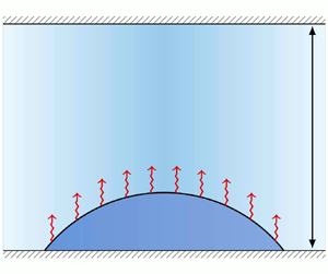
Our present aim is to develop a relatively simple mesoscopic model that bridges cases (i) and (iii) for the specific geometry of a sessile drop of partially wetting liquid evaporating into the narrow gap between two parallel rigid smooth solid plates (see figure 1). For such a narrow gap, the vapour concentration can be vertically averaged allowing us to describe the coupled liquid and vapour dynamics by kinetic equations of reduced dimensions. For simplicity, we consider a completely isothermal system – thermal effects can be incorporated later on.

Figure 1. Sketch of the considered system. It consists of two parallel rigid smooth solid plates separated by a gap of height  $d$. A layer or shallow sessile drop of volatile liquid with a thickness profile $h(\boldsymbol {r},t)$ with $\boldsymbol {r}=(x,y)^{\rm T}$ is situated on the lower plate without touching the upper one. The height-averaged density between the liquid and the upper plate is $\rho (\boldsymbol {r},t)$ for the vapour, and $\rho _{air}(\boldsymbol {r},t)$ for the remaining (inert) gas, i.e. the total height-averaged gas density is $\rho _{tot}=\rho +\rho _{air}$. There can be exchange between the liquid and the vapour due to evaporation/condensation.
We develop the model using a gradient dynamics approach (Thiele Reference Thiele2010, Reference Thiele2018) as employed for other similar systems involving more than one dynamic quantity. Examples include dewetting two-layer liquid films (Pototsky et al. Reference Pototsky, Bestehorn, Merkt and Thiele2004; Jachalski et al. Reference Jachalski, Huth, Kitavtsev, Peschka and Wagner2013), liquid films covered by surfactants (Thiele, Archer & Pismen Reference Thiele, Archer and Pismen2016) and drops spreading on polymer brushes (Thiele & Hartmann Reference Thiele and Hartmann2020). On the one hand, the approach makes the relation between the various contributions to the underlying energy and the different fluxes rather transparent and automatically ensures thermodynamic consistence. This resulting model then automatically covers the diffusion-limited and transfer-limited cases as well as the transition between them. On the other hand, the approach fosters the incorporation of the here developed model for a volatile sessile drop as a building block into a wider class of gradient dynamics models for related more complex settings involving phase change.
Furthermore, we show that the mesoscopic gradient dynamics model favourably compares to a macroscopic description as well as to experiments. Macroscopically, we employ a Stokes model coupled to diffusion in the gas phase. Thereby, an evaporation rate  $j_{evap}$ is implemented into the boundary condition at the liquid–gas interface that is equivalent to the one used in our gradient dynamics model. At the contact line, a Navier slip condition is used. In the gas phase a vapour diffusion model is employed that fully resolves the space within the gap. Versatile variants of this model have been successfully used to account for, e.g. multi-component droplet evaporation (Diddens et al. Reference Diddens, Tan, Lv, Versluis, Kuerten, Zhang and Lohse2017; Li et al. Reference Li, Diddens, Lv, Wijshoff, Versluis and Lohse2019) or droplets evaporating on a thin oil film (Li et al. Reference Li, Diddens, Segers, Wijshoff, Versluis and Lohse2020).
Experimental results on evaporating sessile droplets are extensive (see the reviews by Cazabat & Guena Reference Cazabat and Guena2010; Brutin & Starov Reference Brutin and Starov2018; Zang et al. Reference Zang, Tarafdar, Tarasevich, Choudhury and Dutta2019), but only a limited number of the previous studies investigate the effect of confinement, e.g. inside rectangular microfluidic channels (Bansal, Chakraborty & Basu Reference Bansal, Chakraborty and Basu2017a; Bansal et al. Reference Bansal, Hatte, Basu and Chakraborty2017b; Hatte et al. Reference Hatte, Dhar, Bansal, Chakraborty and Basu2019a), in a box (Shahidzadeh-Bonn et al. Reference Shahidzadeh-Bonn, Rafai, Azouni and Bonn2006), squeezed between two plates (He et al. Reference He, Cheng, Patrick Collier, Srijanto and Briggs2020; Pradhan & Panigrahi Reference Pradhan and Panigrahi2020) or within a gap geometry similar to ours (Basu et al. Reference Basu, Rao, Chattopadhyay and Chakraborty2021). To provide counterpart experiments for our theory, we analyse the evaporation of a droplet between two horizontal plates, where confinement is only imposed in the vertical direction.
This paper is structured as follows. In § 2 we present the theoretical and experimental approaches that are compared in this work. In particular, § 2.1 discusses the general form of gradient dynamics models for one and two scalar fields with combined conserved and non-conserved dynamics. In § 2.2 we derive the gradient dynamics model for the evaporating drop in the considered small gap geometry, and specify all necessary parameters and specific functions. Sections 2.3 and 2.4 briefly introduce the Stokes description and the experimental set-up, respectively. Section 3 presents results obtained with the developed mesoscopic model that, in the subsequent § 4, are compared with Stokes-description results and corresponding experiments. Finally, § 5 concludes with a discussion of the limitations of the presented approach and an outlook toward its further development and application.
2. Models
2.1. Long-wave gradient dynamics models
The dynamics of a layer or shallow drop of non-volatile liquid in long-wave approximation (Oron et al. Reference Oron, Davis and Bankoff1997; Craster & Matar Reference Craster and Matar2009) is characterised by the evolution of a single field – the layer thickness  $h$. As first noted by Oron & Rosenau (Reference Oron and Rosenau1992) and Mitlin (Reference Mitlin1993), the corresponding dynamic equation can be written as gradient dynamics for a conserved field, i.e.
 \begin{equation} \partial_t h =\boldsymbol{\nabla}\, \boldsymbol{\cdot}\, \left(Q\boldsymbol{\nabla}\frac{\delta\mathcal{F}}{\delta h}\right), \end{equation}
where the energy functional  $\mathcal {F}[h]$ contains wetting energy and surface energy of the free liquid–gas interface. Then, its variation represents a pressure consisting of Derjaguin (or disjoining) and Laplace (or curvature) contributions. The function $Q(h)\geqslant 0$ is the positive mobility in the conserved case. Here, $\partial _t$ denotes the partial time derivative and $\boldsymbol {\nabla } = (\partial _x, \partial _y)^{\rm T}$ is the two-dimensional spatial gradient operator.
To account for evaporation, one may add a non-conserved contribution to the dynamics (Lyushnin et al. Reference Lyushnin, Golovin and Pismen2002) and obtain in gradient dynamics form (Thiele Reference Thiele2010, Reference Thiele2018)
 \begin{equation} \partial_t h = \boldsymbol{\nabla}\, \boldsymbol{\cdot}\, \left(Q\boldsymbol{\nabla}\frac{\delta\mathcal{F}}{\delta h}\right) - M\left(\frac{\delta \mathcal{F}}{\delta h} -p_{vap}\right), \end{equation}
where  $M(h)\geqslant 0$ is the non-conserved mobility – for a discussion of different forms, see Thiele (Reference Thiele2014). Thermodynamic consistence is ensured by the positive definiteness of both mobilities and the usage of the same energy in both contributions. In the simplest case, $p_{vap}$ is the imposed constant external vapour pressure in the gas phase implying that (2.2) only models the case of transition-limited evaporation, however, including wettability and capillarity dependencies.
For systems with more degrees of freedom, the described one-field model (2.2) is extended by incorporating the dynamics of further fields (Thiele Reference Thiele2018). In the context of mesoscopic long-wave hydrodynamics, two-field gradient dynamics models are presented and analysed for (i) dewetting two-layer films on solid substrates, i.e. staggered layers of two immiscible fluids (Pototsky et al. Reference Pototsky, Bestehorn, Merkt and Thiele2004, Reference Pototsky, Bestehorn, Merkt and Thiele2005, Reference Pototsky, Bestehorn, Merkt and Thiele2006; Bommer et al. Reference Bommer, Cartellier, Jachalski, Peschka, Seemann and Wagner2013; Jachalski et al. Reference Jachalski, Huth, Kitavtsev, Peschka and Wagner2013); (ii) decomposing and dewetting films of a binary liquid mixture (with non-surface active components) (Thiele Reference Thiele2011; Thiele, Todorova & Lopez Reference Thiele, Todorova and Lopez2013; Diez et al. Reference Diez, González, Garfinkel, Rack, McKeown and Kondic2021); (iii) the dynamics of a liquid film that is covered by an insoluble surfactant (Thiele, Archer & Plapp Reference Thiele, Archer and Plapp2012; Thiele et al. Reference Thiele, Archer and Pismen2016); (iv) the spreading of a liquid drop on a polymer brush (Thiele & Hartmann Reference Thiele and Hartmann2020) and (v) on an elastic substrate without (Henkel, Snoeijer & Thiele Reference Henkel, Snoeijer and Thiele2021) and with (Henkel et al. Reference Henkel, Essink, Hoang, van Zwieten, van Brummelen, Thiele and Snoeijer2022) Shuttleworth effect. In all these cases, the model is of the form
 \begin{equation} \partial_t u_a = \boldsymbol{\nabla} \, \boldsymbol{\cdot}\, \left( \sum_{b=1}^2 {\mathsf{Q}}_{ab} \boldsymbol{\nabla} \frac{\delta \mathcal{F}}{\delta u_b}\right) - \sum_{b=1}^2 {\mathsf{M}}_{ab} \frac{\delta \mathcal{F}}{\delta u_b}, \end{equation}
where the indices  $a, b = 1,2$ refer to the two fields. For the considered relaxational dynamics, the $\boldsymbol{\mathsf{Q}}(u_1,u_2)$ and $\boldsymbol{\mathsf{M}}(u_1,u_2)$ represent $2 \times 2$ positive definite and symmetric mobility matrices for the conserved and non-conserved parts of the dynamics, respectively, written here in terms of their components ${\mathsf{Q}}_{ab}$ and ${\mathsf{M}}_{ab}$. In examples (i) to (iii), both fields show a conserved dynamics, i.e. $\boldsymbol{\mathsf{M}}=0$. However, in general, they can also show a purely non-conserved dynamics, i.e. $\boldsymbol{\mathsf{Q}}=0$ (e.g. the two-field model A in Hohenberg & Halperin Reference Hohenberg and Halperin1977), or a mixed dynamics as in cases (iv) and (v), i.e. $\boldsymbol{\mathsf{M}}, \boldsymbol{\mathsf{Q}}\neq 0$.
The mobilities  $\boldsymbol{\mathsf{Q}}$ enter the fluxes $\boldsymbol j_a=-\sum _{b=1}^2{\mathsf{Q}}_{ab}\boldsymbol {\nabla }({\delta \mathcal {F}}/{\delta u_b})$ of the conserved part of the dynamics for both fields $u_a$. They are given as linear combinations of the influences of both thermodynamic forces $-\boldsymbol {\nabla }({\delta \mathcal {F}}/{\delta u_b})$. The components of $\boldsymbol{\mathsf{M}}$ give the transition rates between the two fields and between the fields and the surroundings. The conserved fields $u_1$ and $u_2$ represent in case (i) the lower layer thickness $h_1$ and overall thickness $h_2$, respectively (Pototsky et al. Reference Pototsky, Bestehorn, Merkt and Thiele2004, Reference Pototsky, Bestehorn, Merkt and Thiele2005; Jachalski et al. Reference Jachalski, Huth, Kitavtsev, Peschka and Wagner2013), or the lower and upper layer thickness (Bommer et al. Reference Bommer, Cartellier, Jachalski, Peschka, Seemann and Wagner2013). In case (ii), $u_1$ and $u_2$ represent the film height $h$ and the effective solute height $\psi =ch$, respectively, where $c$ is the height-averaged solute concentration, while in case (iii), $u_1$ and $u_2$ represent the film height $h$ and the surfactant coverage, respectively (Thiele et al. Reference Thiele, Archer and Plapp2012). Finally, in cases (iv) and (v), $u_1$ represents the drop height while $u_2$ stands for the local amount of liquid in the polymer brush (Thiele & Hartmann Reference Thiele and Hartmann2020) and the elastic–liquid interface profile (Henkel et al. Reference Henkel, Snoeijer and Thiele2021), respectively.
2.2. Gradient dynamics for volatile liquid in small gap geometry
2.2.1. Gradient dynamics form
Having set the stage for formulating mesoscopic models as gradient dynamics on an underlying energy functional, we next introduce such a model for an evaporating sessile liquid drop with profile  $h(\boldsymbol {r},t)$ in a gap of height $d$ (see figure 1). We employ two fields, on the one hand, the amount $\psi _1(\boldsymbol {r},t)$ of the substance in liquid state in the drop per substrate area and, on the other hand, the amount $\psi _2(\boldsymbol {r},t)$ of the substance in vapour form in the gas phase also per substrate area. The field $\psi _1(\boldsymbol {r},t)$ is proportional to the thickness of the liquid film, i.e.
 \begin{equation} \psi_1(\boldsymbol{r},t)= \rho_{liq} h(\boldsymbol{r},t),\end{equation}
where  $\rho _{liq}$ is the constant liquid density (to be specified later). All employed densities are number densities, i.e. are given in units of particles per volume. The field $\psi _2(\boldsymbol {r},t)$ is proportional to the height-averaged vapour density $\rho (\boldsymbol {r},t)$, namely,
 \begin{equation} \psi_2(\boldsymbol{r},t)= \rho(\boldsymbol{r},t) [d-h(\boldsymbol{r},t)]. \end{equation}
The gas phase can either consist of pure vapour or of vapour in an inert gas (called ‘air’ in the following). The latter has height-averaged density  $\rho _{air}(\boldsymbol {r},t)$ and the resulting total gas density is $\rho _{tot}=\rho +\rho _{air}$. The literature distinguishes the following three main cases.
(i) Evaporation into pure vapour treated isothermally. In this case no diffusion occurs, all dynamics in the gas phase is due to pressure equilibration via convective motion. However, this is a very fast process as it occurs with the speed of sound (Maxwell Reference Maxwell1890). On the time scale of evaporation one then assumes uniform vapour, i.e. gas pressure. This implies that $\rho (\boldsymbol {r},t)$ is uniform.
(ii) Evaporation into air treated isothermally. In this case vapour diffusion is very important. As in case (i), the total pressure equilibrates fast, i.e.
$\rho _{tot}$ is constant and uniform, e.g. $p=k_B T \rho _{tot}$ for an ideal gas, where $k_B$ is the Boltzmann constant and $T$ the temperature. In consequence,
(2.6)\begin{equation} \rho_{air}(\boldsymbol{r},t)=\rho_{tot}-\rho(\boldsymbol{r},t) = \rho_{tot}-\frac{\psi_2(\boldsymbol{r},t)}{d-h(\boldsymbol{r},t)}. \end{equation}(iii) As case (i) or case (ii), but not treated isothermally. Then, heat diffusion becomes a limiting factor as the heat used up as latent heat during the liquid–vapour phase transition needs to be transported to the interface. It also becomes important that normally a jump in the heat flux is considered at the interface that ultimately controls the evaporation flux. Here, we will not discuss this case.


Next, we write the model for the coupled dynamics of the local amounts of liquid and vapour in the gradient dynamics form (2.3). In particular, the  $\psi _i$ follow the mixed conserved and non-conserved dynamics
 \begin{equation} \left.\begin{gathered}
\partial_t \psi_1 =
\boldsymbol{\nabla}\, \boldsymbol{\cdot}\, \left({\mathsf{Q}}_{11}\boldsymbol{\nabla}\frac{\delta
\mathcal{F}}{\delta \psi_1} +{\mathsf{Q}}_{12}\boldsymbol{\nabla}\frac{\delta \mathcal{F}}{\delta
\psi_2}\right)- {\mathsf{M}}_{11}\frac{\delta \mathcal{F}}{\delta \psi_1} - {\mathsf{M}}_{12} \frac{\delta \mathcal{F}}{\delta
\psi_2},\\ \partial_t \psi_2 = \boldsymbol{\nabla}\, \boldsymbol{\cdot}\, \left({\mathsf{Q}}_{21}\boldsymbol{\nabla}\frac{\delta
\mathcal{F}}{\delta \psi_1}+ {\mathsf{Q}}_{22}\boldsymbol{\nabla}\frac{\delta \mathcal{F}}{\delta
\psi_2}\right) -{\mathsf{M}}_{21}\frac{\delta \mathcal{F}}{\delta \psi_1}-{\mathsf{M}}_{22}\frac{\delta \mathcal{F}}{\delta \psi_2}.
\end{gathered}\right\}\end{equation}
\begin{equation} \left.\begin{gathered}
\partial_t \psi_1 =
\boldsymbol{\nabla}\, \boldsymbol{\cdot}\, \left({\mathsf{Q}}_{11}\boldsymbol{\nabla}\frac{\delta
\mathcal{F}}{\delta \psi_1} +{\mathsf{Q}}_{12}\boldsymbol{\nabla}\frac{\delta \mathcal{F}}{\delta
\psi_2}\right)- {\mathsf{M}}_{11}\frac{\delta \mathcal{F}}{\delta \psi_1} - {\mathsf{M}}_{12} \frac{\delta \mathcal{F}}{\delta
\psi_2},\\ \partial_t \psi_2 = \boldsymbol{\nabla}\, \boldsymbol{\cdot}\, \left({\mathsf{Q}}_{21}\boldsymbol{\nabla}\frac{\delta
\mathcal{F}}{\delta \psi_1}+ {\mathsf{Q}}_{22}\boldsymbol{\nabla}\frac{\delta \mathcal{F}}{\delta
\psi_2}\right) -{\mathsf{M}}_{21}\frac{\delta \mathcal{F}}{\delta \psi_1}-{\mathsf{M}}_{22}\frac{\delta \mathcal{F}}{\delta \psi_2}.
\end{gathered}\right\}\end{equation}
Note, however, that  $h$ is the relevant field for many of the physical effects and that often it may be more convenient to write the governing equations in terms of $h$ (2.4) and $\psi =\psi _2$.
First, we focus on case (ii) before discussing the amendments needed for case (i). As on the considered time scales, the total gas pressure is uniform, there is no pressure gradient that would drive convective transport in the gas phase. In consequence, there is no dynamic coupling between the liquid and gas layer, i.e.  ${\mathsf{Q}}_{12}={\mathsf{Q}}_{2 1}=0$. Transport in the gas phase is then limited to vapour diffusion within the air. As a result, the conserved mobilities are
 \begin{equation} \boldsymbol{\mathsf{Q}}=\left(\begin{array}{cc} \dfrac{1}{\rho_{liq}}\,\dfrac{\psi_1^3}{3 \eta} & 0 \\[8pt] 0 & \tilde{D} \psi_2 \end{array}\right),\end{equation}
where  $\eta$ is the dynamic viscosity of the liquid and $\tilde {D}$ is a diffusive mobility constant. We obtain ${\mathsf{Q}}_{11}$ by considering the standard long-wave evolution equation (Oron et al. Reference Oron, Davis and Bankoff1997; Craster & Matar Reference Craster and Matar2009). We multiply its gradient dynamics formulation (Thiele Reference Thiele2010) by the liquid density $\rho _{liq}$ and replace $h$ by $\psi _1/\rho _{liq}$ to obtain
 \begin{equation} \partial_t \psi_1 = \rho_{liq}\partial_t h = \rho_{liq} \boldsymbol{\nabla}\, \boldsymbol{\cdot}\, \left(\frac{h^3}{3 \eta}\boldsymbol{\nabla} \frac{\delta \mathcal{F}}{\delta h}\right) = \boldsymbol{\nabla}\, \boldsymbol{\cdot}\, \left({\mathsf{Q}}_{11} \boldsymbol{\nabla}\frac{\delta \mathcal{F}}{\delta \psi_1}\right). \end{equation}
The form of the diffusive mobility  ${\mathsf{Q}}_{22}$ is for dilute solutions discussed by Thiele (Reference Thiele2011) and Xu, Thiele & Qian (Reference Xu, Thiele and Qian2015). The presently employed form $\tilde {D} \psi _2=\tilde {D} (d-h)\rho$ is the direct equivalent for the present case of vapour diffusion in the gap between the liquid and upper wall. It can be related to the usual diffusion constant $D$ of the vapour particles in air by $D = k_B T \tilde {D}$.
In the simplest case, the non-conserved mobilities are
 \begin{equation} \boldsymbol{\mathsf{M}} = \tilde{M}\left(\begin{array}{cc} 1 & -1 \\ -1 & 1 \end{array} \right),\end{equation}
where  $\tilde {M}$ is an evaporation rate constant, which can be estimated, e.g. from the Hertz–Knudsen equation (Knudsen Reference Knudsen1915; Librovich et al. Reference Librovich, Nowakowski, Nicolleau and Michelitsch2017), which linearly incorporates an accommodation (or ‘sticking’) coefficient of the gas molecules. Note that more intricate models for phase change may be implemented via the non-conserved terms, e.g. by employing a variable evaporation rate $\tilde {M}(\psi _1, \psi _2)$. Our choice in (2.10) represents the simplest case for an evaporation that is purely driven by the differences in chemical potentials. Moreover, the particular matrix (2.10) ensures that the total particle number $\int (\psi _1+\psi _2)\,\mathrm{d}\kern0.7pt x\,\mathrm {d} y$ is conserved, i.e. $\psi _1+\psi _2$ satisfies the continuity equation $\partial _t (\psi _1+\psi _2)= \boldsymbol {\nabla }\boldsymbol {{\cdot }}(\,\boldsymbol {j}_{\psi _1}+\boldsymbol {j}_{\psi _2})$.
The free energy in long-wave approximation is
 \begin{equation} \mathcal{F} \!=\! \int_\varOmega \left[\underbrace{\gamma\left(1+\frac{|\boldsymbol{\nabla} h|^2}{2}\right)}_{\mathrm{surface}} +\! \underbrace{g(h)}_{\text{wetting}} +\!\underbrace{h f_{liq}(\rho_{liq})}_{\text{liquid bulk}} +\underbrace{(d\!-\!h) f_{vap}(\rho)}_{\text{vapour bulk}} +\underbrace{(d\!-\!h) f_{air}(\rho_{air})}_{\text{air bulk}} \right] \mathrm{d}\kern0.7pt x\,\mathrm{d} y, \end{equation}
where the  $f_i$'s are bulk liquid, vapour and air energies per volume, $\gamma$ is the liquid–gas interface tension and $g(h)$ is the wetting energy per area. The functional is accompanied by the constraint of particle number conservation across the two phases. The condition is
 \begin{equation} 0 = \int_\varOmega \left[\psi_1 + \psi_2 - \bar{n}\right]\mathrm{d}\,\boldsymbol{x} = \int_\varOmega \left[h \rho_{liq} + (d-h) \rho -\bar{n}\right] \mathrm{d}\kern0.7pt x\,\mathrm{d} y, \end{equation}
where  $\bar {n}$ is the mean (liquid and vapour) particle number per substrate area. Here, particle flux through the boundaries of the domain $\varOmega$ is excluded, however, it can be easily incorporated. Also, gravity is neglected as we consider small droplets, but may be added in the form of potential energy.
The presented long-wave formulation of the mesoscopic model is best suited for shallow droplets. However, as briefly discussed in § 3 of Thiele (Reference Thiele2018), it is an advantage of the gradient dynamics formulation that one may separately discuss improvements of the energy functional and the mobilities. There, it is argued that a good strategy for model improvements consists in making the energy as exact as possible and keeping the mobilities as simple as possible. Here, in particular, we may use a full-curvature trick similar to Gauglitz & Radke (Reference Gauglitz and Radke1988), Snoeijer et al. (Reference Snoeijer, Andreotti, Delon and Fermigier2007) and von Borries Lopes, Thiele & Hazel (Reference von Borries Lopes, Thiele and Hazel2018) that allows us to study the evaporation of droplets with larger contact angles. In practice, this is achieved by writing the surface energy term in (2.11) with the full metric factor  $\gamma \sqrt {1+(\boldsymbol {\nabla } h )^2}$. Here, we also improve the non-conserved mobilities by accordingly replacing the evaporation rate per surface area $\tilde {M}$ in (2.10) by $\tilde {M}\sqrt {1+(\boldsymbol {\nabla } h )^2}$. Below we will refer to this amendment as the full-curvature formulation of the mesoscopic model. For brevity, in the following we refer to the standard long-wave formulation of the mesoscopic model as the ‘long-wave model’. Although experience shows that the described energy-focused strategy can even correct qualitatively incorrect results of a long-wave description (von Borries Lopes et al. Reference von Borries Lopes, Thiele and Hazel2018), and is also applied in descriptions like the Cahn–Hilliard model (Cahn Reference Cahn1965) for the decomposition of a binary mixture (Thiele Reference Thiele2018), it should be noted that the approach may be considered as not being ‘rational’ in an asymptotic sense: part of the neglected terms are of the same order in the smallness parameter of the long-wave approximation as the included improvements of the energy.
Furthermore, we remark that (2.11) is in a somewhat mixed form as it considers at the same time equations of state encoded in the  $f$'s for liquid and vapour that may result in phase change, but also uses the film height $h$ as it is the most important quantity for mesoscopic hydrodynamics. As stated above, we treat $\rho _{liq}$ as constant and will consider the vapour as an ideal gas. This is the result of a two-step procedure, explained in the next section (that may be skipped by the reader who is mainly interested in the resulting system of equations).
2.2.2. From real to ideal vapour
An equation of state for a real gas, e.g. a van der Waals gas, predicts coexisting liquid and vapour densities at equilibrium. In an out-of-equilibrium hydrodynamic description, liquid and vapour densities may vary in space and time. However, there is no unique way to express the three fields  $\rho _{liq}(\boldsymbol {r},t), \rho (\boldsymbol {r},t)$ and $h(\boldsymbol {r},t)$ in terms of the two fields $\psi _1 (\boldsymbol {r},t)$ and $\psi _2 (\boldsymbol {r},t)$ that our gradient dynamics (2.7) is based on. Therefore, we introduce the following two-step procedure of simplifications that allows us to treat $\rho _{liq}$ as a constant.
(i) We assume a thick homogeneous sharp-interface flat film of thickness  $h$, i.e. the energy functional (2.11) becomes
 \begin{equation} \mathcal{F}_0[\rho_{liq}, \rho_{vap}] = \int_\varOmega \left[ h f_{liq}(\rho_{liq}) +(d-h) f_{vap}(\rho_{vap}) \right] \mathrm{d}\kern0.7pt x\,\mathrm{d} y, \end{equation}
where we also dropped the constant  $\gamma$. To calculate $\rho _{liq}$ and $\rho _{vap}$ at coexistence (as functions of temperature $T$), we minimise
 \begin{align} \mathcal{F}_1[\rho_{liq}, \rho_{vap},h,\xi] &= \int_\varOmega \left[ h f_{liq}(\rho_{liq}) +\xi f_{vap}(\rho_{vap}) \right] \mathrm{d}\,x\,\mathrm{d} y\nonumber\\ &\quad - \tilde \mu \int_\varOmega \left[h \rho_{liq} + \xi \rho -\bar{n}\right]\mathrm{d}\,x\,\mathrm{d} y + \tilde{p} \int_\varOmega \left[h + \xi - d\right]\mathrm{d}\kern0.7pt x\,\mathrm{d} y \end{align}
with respect to  $\rho _{liq}, \rho _{vap},h$ and $\xi =d-h$ that we treat as an independent field. Here, $\tilde {\mu }$ and $\tilde {p}$ are Lagrange multipliers for mass and volume conservation. We obtain
 \begin{equation} \left.\begin{gathered} \tilde{\mu} = f'_{liq}(\rho_{liq}) = f'_{vap}(\rho_{vap}),\\ \tilde{p} = f_{liq}(\rho_{liq}) - \tilde{\mu}\rho_{liq} = f_{vap}(\rho_{vap}) - \tilde{\mu}\rho_{vap}, \end{gathered}\right\} \end{equation}
i.e. the standard Maxwell construction for phase coexistence. These we use to obtain the coexisting  $\rho _{liq}$ (and, therefore, $f_{liq}$) and $\rho _{vap}$ analytically or (most likely) numerically. (To do so, we either employ a single function $f=f_{vap}=f_{liq}$ that allows for a liquid–gas phase transition (e.g. the van der Waals free energy) or combine a purely entropic $f_{vap}(\rho ) = k_B T \rho [\log (\varLambda ^3 \rho )-1]$ with an $f_{liq}(\rho )$ that allows for a phase transition.) For the considered isothermal system, this fixes $\rho _{liq}$, $\rho _{vap}$ and $f_{liq}$ at coexistence values.
(ii) Next we approximate the equation of state in the vapour and the liquid phase. For the liquid phase, we neglect any compressibility, i.e. we fix the density in the liquid layer to  $\rho _{liq}$. In other words, the ‘liquid branch’ of the equation of state $p(\rho )$ is replaced by a vertical line at $\rho =\rho _{liq}$. The ‘gas branch’ of the equation of state is either directly replaced by the ideal gas law given above or, alternatively, is expanded up to linear order about $\rho =\rho _{vap}$. This results in a shifted and scaled ideal gas law. The latter approach has the advantage that coexistence pressure and concentration are exactly as in the equation of state one started with.
In this way the relation  $h=\psi _1/\rho _{liq}$ introduced above becomes meaningful and the relation of the variations with respect to $h$ and to $\psi _1$ alluded to earlier is justified. Also using $\rho =\psi _2/(d-h)$, the free energy functional (2.11) is written as
 \begin{align} \mathcal{F}[\psi_1,\psi_2] &= \int_\varOmega \left[\frac{\gamma}{2 \rho_{liq}^2} {(\boldsymbol{\nabla} \psi_1)}^2 + g\left(\frac{\psi_1}{\rho_{liq}}\right) +\frac{f_{liq}}{\rho_{liq}} \psi_1 +\left(d-\frac{\psi_1}{\rho_{liq}}\right) f_{vap}\left(\frac{\psi_2}{d-\psi_1/\rho_{liq}}\right) \right.\nonumber\\ &\quad \left. +\left(d-\frac{\psi_1}{\rho_{liq}}\right) f_{air}\left(\rho_{tot}-\frac{\psi_2}{d-\psi_1/\rho_{liq}}\right) \right] \mathrm{d}\,x\,\mathrm{d} y. \end{align}
Here, it only depends on  $\psi _1$ and $\psi _2$. Note that $f_{liq}$ is now a constant given, for instance, by the Maxwell construction as explained above. Alternatively, one may directly deduce the value of $f_{liq}$ from the saturation pressure of the liquid by considering the equilibrium state of a liquid film in a saturated atmosphere as done here in § 2.2.4, resulting in (2.29).
2.2.3. Evolution equations
Here, we bring all the information discussed in the previous sections together and present the resulting long-wave model.
The energy functional (2.16) in terms of  $\psi _1$ and $\psi _2$ is now minimised together with the particle number constraint (2.12) (Lagrange multiplier $\mu$) with respect to variations in the two fields. This gives
 \begin{align} \frac{\delta \mathcal{F}}{\delta \psi_1} &= \frac{1}{\rho_{liq}} \left[ -\gamma\Delta h + g'\left(h\right) +f_{liq} -f_{vap}(\rho)+ \rho f_{vap}'(\rho)\right.\nonumber\\ &\quad\left.\vphantom{-\gamma\Delta h + g'\left(h\right) +f_{liq} -f_{vap}(\rho)+ \rho f_{vap}'(\rho)} - f_{air}(\rho_{tot}-\rho) - \rho f_{air}'(\rho_{tot}-\rho)\right] - \mu, \end{align}
where the brackets contain Laplace pressure, Derjaguin pressure, liquid energy and vapour pressure. Note that the somewhat unusual final contribution to the vapour pressure is a direct consequence of the assumption of constant  $p_{tot}$. Here and in the following, we use $h$ and $\rho$ as abbreviations where appropriate.
The variation with respect to  $\psi _2$ gives
 \begin{equation} \frac{\delta \mathcal{F}}{\delta \psi_2} =f_{vap}'(\rho) - f_{air}' (\rho_{tot}-\rho) - \mu, \end{equation}
i.e. a difference in chemical potentials. If we now specify vapour and air to be ideal gases,  $f_{vap}=k_B T \rho [\log (\varLambda ^3 \rho )-1]$ and $f_{air}=k_B T \rho _{air}[\log (\varLambda ^3 \rho _{air})-1]$ with the mean free path length $\varLambda$, we obtain
 \begin{equation} \frac{\delta \mathcal{F}}{\delta \psi_1} = \frac{1}{\rho_{liq}} \left\{-\gamma\Delta h+ g'(h) +f_{liq} + k_B T\rho_{tot} - k_B T\rho_{tot} \log[\varLambda^3 (\rho_{tot}-\rho)]\right\} - \mu. \end{equation}
The gradient of this pressure drives the dynamics in the liquid film. The constant liquid energy density  $f_{liq}$ and the constant ideal pressure $k_BT\rho _{tot}$ do not contribute to the conserved dynamics, but the final term in the curly parenthesis does. It is a direct consequence of treating case (ii), i.e. of imposing a uniform gas pressure, that is, constant $\rho _{tot}$. The other variation is then
 \begin{equation} \frac{\delta \mathcal{F}}{\delta \psi_2} =k_B T \{\log(\varLambda^3 \rho) - \log[\varLambda^3 (\rho_{tot}-\rho)]\} - \mu. \end{equation}
Also here the second term in the curly parenthesis is a consequence of the imposed uniform pressure in case (ii).
Introducing the obtained expressions into the general two-field gradient dynamics (2.7) with (2.8) and (2.10) gives
 \begin{gather}
\partial_t \psi_1 =
\boldsymbol{\nabla}\, \boldsymbol{\cdot}\, \left(\frac{\psi_1^3}{3
\rho_{liq}^2\eta}\boldsymbol{\nabla} \left\{ -\gamma \Delta
h + g'\left(h\right)- k_B T\rho_{tot}
\log[\varLambda^3(\rho_{tot}-\rho)] \right\}\right) -
\tilde{M}E,\nonumber\\ \partial_t \psi_2 =
\boldsymbol{\nabla}\, \boldsymbol{\cdot}\, \left(\tilde{D} k_B
T
\frac{d-h}{1-\rho/\rho_{tot}}\boldsymbol{\nabla}\rho\right)
+ \tilde{M} E,\nonumber\\ \mathrm{where}\ E=\frac{1}{\rho_{liq}}
\left[-\gamma \Delta h + g'(h)+f_{liq}\right]\nonumber\\ + k_B T
\left\{ \frac{\rho_{tot}}{\rho_{liq}} +\left(1-
\frac{\rho_{tot}}{\rho_{liq}}\right)
\log[\varLambda^3(\rho_{tot}-\rho)] - \log(\varLambda^3
\rho) \right\}.
\end{gather}
\begin{gather}
\partial_t \psi_1 =
\boldsymbol{\nabla}\, \boldsymbol{\cdot}\, \left(\frac{\psi_1^3}{3
\rho_{liq}^2\eta}\boldsymbol{\nabla} \left\{ -\gamma \Delta
h + g'\left(h\right)- k_B T\rho_{tot}
\log[\varLambda^3(\rho_{tot}-\rho)] \right\}\right) -
\tilde{M}E,\nonumber\\ \partial_t \psi_2 =
\boldsymbol{\nabla}\, \boldsymbol{\cdot}\, \left(\tilde{D} k_B
T
\frac{d-h}{1-\rho/\rho_{tot}}\boldsymbol{\nabla}\rho\right)
+ \tilde{M} E,\nonumber\\ \mathrm{where}\ E=\frac{1}{\rho_{liq}}
\left[-\gamma \Delta h + g'(h)+f_{liq}\right]\nonumber\\ + k_B T
\left\{ \frac{\rho_{tot}}{\rho_{liq}} +\left(1-
\frac{\rho_{tot}}{\rho_{liq}}\right)
\log[\varLambda^3(\rho_{tot}-\rho)] - \log(\varLambda^3
\rho) \right\}.
\end{gather}
This is the final result for case (ii).
Then, the saturation vapour density  $\rho _{sat}$ above a flat thick film is obtained by setting the transfer term to zero ( $E=0$) and dropping capillarity and wettability influences, i.e.
 \begin{equation} E = \frac{f_{liq}}{\rho_{liq}} + k_B T \left\{ \frac{\rho_{tot}}{\rho_{liq}} +\left(1- \frac{\rho_{tot}}{\rho_{liq}}\right) \log[\varLambda^3(\rho_{tot}-\rho_{sat})] - \log(\varLambda^3 \rho_{sat}) \right\}=0. \end{equation}
The corresponding film height  $H$ is determined by the conservation of mass ${\bar {n} = \psi _1+\psi _2 = H \rho _{liq} + (d-H)\rho _{sat}}$.
Note that the somewhat unexpected terms related to  $\rho _{tot}$ in the two kinetic equations (2.21) turn out to be well behaved: the additional contributions in the equation for $\psi _2$ provide a factor $1/[1-\rho /\rho _{tot}]$ to the generalized diffusion constant. Normally, $\rho /\rho _{tot}\ll 1$ and might be neglected. If, however, $\rho /\rho _{tot}\to 1$, we approach the limit of pure vapour, where diffusion is not the proper transport process any more: the factor in question diverges, i.e. $\rho$ becomes instantaneously uniform. The additional logarithmic term in the equation for $\psi _1$ corresponds to a flux proportional to $(\boldsymbol {\nabla }\rho )/(1-\rho /\rho _{tot})$. For $\rho /\rho _{tot} \ll 1$, this is the gradient in partial vapour pressure that drives some flow in the adjacent liquid layer, one can see it as an ‘osmotic coupling’. It is normally very small as compared with the other pressure gradients. The local evaporation rate $\tilde {M}E$ contains additional terms proportional to the ratio of total gas density and liquid density $\rho _{tot}/\rho _{liq}$ that we expect to be small. For dry air and water, the ratio is about $10^{-3}$, and humid air has an even lower density than dry air.
For  $\rho /\rho _{tot}\ll 1$ and $\rho _{tot}/\rho _{liq}\ll 1$, (2.21) written in terms of $h$ and $\rho$ reduce to
 \begin{equation} \left.\begin{gathered} \partial_t h ={-}\boldsymbol{\nabla}\, \boldsymbol{\cdot}\, \left\{\frac{h^3}{3 \eta}\boldsymbol{\nabla} \left[ \gamma \Delta h - g'\left(h\right) \right]\right\}- j_{evap},\\ \partial_t[(d-h)\rho] = \boldsymbol{\nabla}\, \boldsymbol{\cdot}\, \left[D (d-h) \boldsymbol{\nabla}\rho\right] + \rho_{liq} j_{evap},\\ \mathrm{where}\ j_{evap}/M ={-}\gamma \Delta h + g'(h)+f_{liq} - \rho_{liq} k_B T \log\left(\frac{\rho}{\rho_{tot}-\rho}\right). \end{gathered}\right\}\end{equation}
Here, we have introduced the diffusion constant  $D = \tilde {D} k_B T$ and the evaporation rate constant of $M = \tilde {M} / \rho _{liq}^2$, thus converting the local particle evaporation rate $\tilde {M} E$ into a volume rate $j_{evap} = \tilde {M} E / \rho _{liq}$. Equation (2.23) allows one to study the crossover between transition-limited drop evaporation dynamics (small $\rho$) and diffusion-limited evaporation dynamics ( $\rho$ at drop close to saturation $\rho _{sat}$).
Before discussing limiting cases and applying our model to study evaporating drops, we briefly compare it to existing models. Equation (2.21) or the simplified (2.23) represents a seamless reduced model for the evaporation of a sessile droplet in a gap. It captures both limiting cases individually considered by Murisic & Kondic (Reference Murisic and Kondic2011). It is of lower complexity than Sultan et al. (Reference Sultan, Boudaoud and Ben Amar2005) as in the description of liquid and vapour the vertical dimension has been eliminated. Its gradient dynamics form makes it transparent and allows for versatile adaptation to many situations, as further discussed in the conclusion.
In case (ii) considered up to here, convective motion in the gas layer is neglected assuming a uniform total gas pressure  $p_{tot}$, i.e. a uniform total gas density ${\rho _{tot}=\rho _{air}+\rho }$ that is an externally controlled parameter of the system. However, this directly couples $\rho _{air}$ to the vapour density $\rho$ and implies the discussed small additional contributions to the pressure in the liquid, to the evaporation/condensation rate and vapour diffusion. In other words, these terms are direct consequences of the gradient dynamics structure. Although, normally, one may neglect them due to their smallness, one needs to keep in mind that ultimately this breaks the thermodynamic consistency and, therefore, may result in unphysical behaviour.
If we consider case (i), evaporation into pure vapour, diffusion is excluded right from the beginning. As in case (ii), we assume that convective motion is very much faster than evaporation, what directly implies that the vapour density  $\rho$ is uniform in the entire gas layer. It is set by the conditions at the lateral boundaries of the gap. In other words, the vapour pressure is then a given constant and the governing equation in gradient dynamics form is (2.2). The corresponding energy is (2.11) without the air energy, without the constant $\gamma$ and with constant $\rho =\rho _{vap}$, i.e.
 \begin{equation} \mathcal{F} = \int_\varOmega \left[ \frac{\gamma}{2} {(\boldsymbol{\nabla} h)}^2 + g(h) +h f_{liq}(\rho_{liq})+(d-h) f_{vap}(\rho_{vap}) \right] \mathrm{d}\,x\,\mathrm{d} y.\end{equation}
Minimisation with respect to film thickness gives
 \begin{equation} \frac{\delta \mathcal{F}}{\delta h} ={-}\gamma\Delta h+ g'(h) + f_{liq} - f_{vap}, \end{equation}
i.e. (2.2) becomes
 \begin{equation} \partial_t h={-}\boldsymbol{\nabla}\, \boldsymbol{\cdot}\, \left\{Q\boldsymbol{\nabla} [\gamma\Delta h - g'(h)] \right\} + M\left[\gamma\Delta h - g'(h) - f_{liq} + f_{vap} + p_{vap}\right]. \end{equation}
Grouping all constants (  $f_{liq}, f_{vap}, p_{vap}$) in the evaporation term into a single one, the equation corresponds to the long-wave description in the transition-limited case (Pismen Reference Pismen2004; Thiele Reference Thiele2010) where evaporation/condensation is controlled by the difference between the sum of Laplace and Derjaguin pressure in the liquid and the constant and uniform imposed vapour pressure.
2.2.4. Specific functions and parameters
One may now proceed by non-dimensionalising, thereby using sensible values of  $\rho _{liq}$ and $f_{liq}$ as parameters. However, as they are not independent, this may result in artefacts. The better approach is to employ a specific equation of state/free energy that allows for liquid–gas phase transition and calculate these values for a particular temperature $T$.
$T$.
An example is the van der Waals equation of state, see, e.g. Landau & Lifshitz (Reference Landau and Lifshitz1980, §§ 76 and 84) giving the pressure
 \begin{equation} p_{vdW}=\frac{k_B T\rho}{1-b\rho}-a\rho^2, \end{equation}
where  $a$ and $b$ are constants (attraction strength and effective excluded volume, respectively). Approximated, in the gas phase with $a,b\to 0$ it becomes the ideal gas law $p_{id}=k_B T\rho$. The corresponding Helmholtz free energy per volume is
 \begin{equation} f_{vdW}={-}k_B T \rho\left[\log\left(\frac{1-\rho b}{\varLambda^3\rho}\right) + 1 \right]-a\rho^2, \end{equation}
becoming  $f_{id}=k_B T \rho [\log (\varLambda ^3\rho ) - 1 ]$ for $a,b\to 0$. Note that $p=-f+\rho f'= \rho ^2\partial_\rho (f(\rho )/\rho )$.
Furthermore, the saturation vapour density  $\rho _{sat}$ follows from the equilibrium condition, e.g. in the simple case of a thick flat liquid film (no Laplace and Derjaguin pressure) setting the evaporation rate to zero in (2.23),
 \begin{equation} j_{evap}/M = f_{liq} - \rho_{liq} k_B T \log\left(\frac{\rho_{sat}}{\rho_{tot}-\rho_{sat}}\right) = 0.\end{equation}
The saturation vapour pressure  $p_{sat}$ resulting from the equation of state may then be used to express the humidity as $\phi = p / p_{sat}$.
If one assumes a specific wetting potential  $g(h)$ that allows for partial wetting, a second spatially homogeneous equilibrium state is found typically at very small height $h_a$ that corresponds to a microscopic adsorption layer
 \begin{equation} g'(h_a) = \rho_{liq}k_B T \log\left(\frac{\rho}{\rho_{tot}-\rho}\right) - f_{liq}.\end{equation}
The height  $h_a$ depends on the vapour density $\rho$ and will be slightly shifted from the height $h_p$ where the Derjaguin pressure vanishes ( $g'(h_p) = 0$), i.e. the adsorption layer height of the saturated case $h_p = h_a(\rho _{sat})$. In fact, this allows for a set of spatially homogeneous equilibrium states, where the vapour density is an arbitrary constant $0 < \rho \leqslant \rho _{sat}$ controlled externally, e.g. by the humidity of the laboratory, while the substrate is macroscopically dry (the ‘moist case’ of de Gennes Reference de Gennes1985) with $h = h_a$. Note that due to the saturation conditions (2.29) and (2.30), we find that $g'(h_a) \leqslant 0$, i.e. the adsorption layer height is shifted to lower values $h_a \leqslant h_p$. When, on the other hand, an initial $\rho (\boldsymbol {r}, t) \geqslant \rho _{sat}$ is given, no equilibrium is guaranteed to exist (depending on the choice of the wetting potential). The evaporation rate $E$ will then become negative leading to a transfer of material from the vapour phase to the liquid film, i.e. condensation.
In the following, we use the simple wetting potential for partially wetting liquids
 \begin{equation} g(h) = \frac{H_A}{2h^2} \left(\frac{2 h_p^3}{5 h^3} - 1\right),\end{equation}
with the Hamaker constant  $H_A \approx 5/3\gamma h_p^2 \theta _e^2$ that relates to the macroscopic equilibrium contact angle $\theta _e$ by a mesoscopic Young's law: $\cos \theta _e = 1 + g(h_p)/\gamma$ (Churaev Reference Churaev1995).
For the simulation of the long-wave model in § 3, we use the following set of realistic parameters (unless stated otherwise): initial drop height  $h_0 = h(r=0, t=0)={1}\ \textrm {mm}$, gap height $d={3}\ \textrm {mm}$, precursor film thickness $h_p = h_0/1000$, diffusion constant $D = \tilde {D} k_B T = 2.8\times 10^{-5}\ \textrm {m}^2\ \textrm {s}^{-1}$ (Lee & Wilke Reference Lee and Wilke1954; Marrero & Mason Reference Marrero and Mason1972), temperature $T={22}\,^{\circ }\textrm {C}$, contact angle $\theta _e = {44.38}^{\circ }$ and a domain radius of $L={25}\ \textrm {mm}$. The liquid properties are chosen according to water at room temperature: viscosity $\eta = 8.9\times 10^{-4}\ \textrm {Pa}\ \textrm {s}$, surface tension $\gamma = 72\times 10^{-3}\ \textrm {N}\ \textrm {m}^{-1}$, particle density according to mass density and molar mass $\rho _{liq} = ({997}\ \textrm {kg}\ \textrm {m}^{-3})/({18}\ \textrm {kg}\ \textrm {mol}^{-1})\,N_A$, and the saturation vapour pressure $p_{sat}={2643}\ \textrm {Pa}$. The parameter values are extracted from Lide (Reference Lide2004). The constant of phase change $M$ is employed as a free parameter that allows us to move between the different limiting cases.
2.2.5. Radial symmetry and numerical implementation
For an efficient numerical simulation of the dynamics, we consider a radial symmetry, i.e. for the long-wave model,  $h(\boldsymbol {x}, t) = h(r, t)$ and $\psi (\boldsymbol {x}, t) = \psi (r, t)$. This allows us to reduce (2.23) to a spatially one-dimensional model in polar coordinates,
 \begin{gather}
\partial_t h = \left(\partial_r + \frac{1}{r}\right)
\left\{\frac{h^3}{3 \eta}\partial_r \left[-\gamma \left(
\partial_r^2 h + \frac{1}{r} \partial_r h \right) +
g'\left(h\right) \right]\right\} - j_{evap},\nonumber\\
\partial_t[(d-h)\rho] = \left(\partial_r +
\frac{1}{r}\right) \left[D (d-h) \partial_r \rho\right] +
\rho_{liq} j_{evap},\nonumber \\ \mathrm{where}\ j_{evap}/M
={-}\gamma \left( \partial_r^2 h + \frac{1}{r} \partial_r h
\right) + g'(h)+f_{liq}- \rho_{liq}k_B T
\log\left(\frac{\rho}{\rho_{tot}-\rho}\right).\end{gather}
\begin{gather}
\partial_t h = \left(\partial_r + \frac{1}{r}\right)
\left\{\frac{h^3}{3 \eta}\partial_r \left[-\gamma \left(
\partial_r^2 h + \frac{1}{r} \partial_r h \right) +
g'\left(h\right) \right]\right\} - j_{evap},\nonumber\\
\partial_t[(d-h)\rho] = \left(\partial_r +
\frac{1}{r}\right) \left[D (d-h) \partial_r \rho\right] +
\rho_{liq} j_{evap},\nonumber \\ \mathrm{where}\ j_{evap}/M
={-}\gamma \left( \partial_r^2 h + \frac{1}{r} \partial_r h
\right) + g'(h)+f_{liq}- \rho_{liq}k_B T
\log\left(\frac{\rho}{\rho_{tot}-\rho}\right).\end{gather}
The dynamic equations are then solved using the finite-element method implemented in the C $++$ library oomph-lib (Heil & Hazel Reference Heil and Hazel2006), which employs a second-order backward differentiation formula for temporal integration. In particular, the library provides both spatial and temporal adaptivity, which is essential due to the multi-scale character of the dynamics, e.g. when spatially resolving the fields in the bulk and near the contact line. In the simulations, the domain is typically discretised with ${\approx }1000$ grid points with spacings that range from $2^{-7}$ to $2^{-18}$ times the domain size.
In these calculations, we employ an adsorption layer of height  $h_p$ that is by a factor of $10^3$ smaller than the initial drop height $h(r=0, t=0)$. Larger ratios are possible but result in a strongly increasing numerical effort. As the effective adsorption layer height is coupled to the gas phase (see, e.g. (2.30)), the overall pressure balance can cause liquid transport through the layer during equilibration. The resulting fluxes are negligible if the adsorption layer is very thin compared with the droplet size. The effect can be further suppressed by modulating the evaporation rate coefficient $M(h)$ with a (smooth) step function, effectively disabling evaporation from the adsorption layer. This is particularly important on the slow time scale of droplet evaporation.
To ensure smoothness of all fields at the drop centre ( $r=0$), we employ natural (homogeneous) Neumann boundary conditions
 \begin{equation} \left.\partial_r h\right|_{r=0} = 0, \quad\left.\partial_r \frac{\delta \mathcal{F}}{\delta \psi_1}\right|_{r=0} = 0 \quad\text{and}\quad \left.\partial_r [(d-h)\rho]\right|_{r=0} = 0.\end{equation}
These conditions also ensure zero liquid and vapour flux through the computational domain boundary at  $r=0$. At the outer boundary far from the drop the gap between the plates is open, i.e. air and vapour can freely be exchanged with the surrounding laboratory. Thus, we assume a constant lab humidity (or vapour concentration) $\rho _{lab}$ corresponding to a Dirichlet boundary conditions at $r=L$. Together with natural Neumann boundary conditions for the film profile $h$ and the chemical potential $\delta \mathcal {F} / \delta \psi _1$, this gives the remaining boundary conditions
 \begin{equation} \left.\partial_r h\right|_{r=L} = 0, \quad\partial_r \left.\frac{\delta \mathcal{F}}{\delta \psi_1}\right|_{r=L} = 0 \quad\text{and}\quad \rho|_{r=L} = \rho_{lab}.\end{equation}
In particular, these conditions allow for a non-zero vapour flux through the outer boundary into the laboratory environment. The external vapour concentration is here chosen such that it corresponds to a low relative humidity of, i.e.,  $\rho _{lab}/\rho _{sat} = 0.1$.
Results obtained with the developed long-wave model are presented in § 3. In the subsequent § 4 they are compared with Stokes-equation results and corresponding experiments.
2.3. Stokes description
Next, we develop a description in terms of the Stokes equation for volatile liquids in the gap geometry again taking into account diffusion processes in the gas phase and the mass transfer at the liquid–gas interface. This will allow us to study the transition between transfer-limited and diffusion-limited cases also in the macroscale model. Then, important cases are compared with the model developed above.
The Stokes equations are solved on an axisymmetric domain, i.e. for the velocity field  $\boldsymbol {u}(r,z,t)$ and the pressure $p(r,z,t)$, we solve
 \begin{gather} -\boldsymbol{\nabla} p + \eta \boldsymbol{\nabla}\, \boldsymbol{\cdot}\, \left[\boldsymbol{\nabla} \boldsymbol{u}+(\boldsymbol{\nabla}\boldsymbol{u})^{\rm T}\right] =0, \end{gather}
 \begin{gather}\boldsymbol{\nabla}\, \boldsymbol{\cdot}\, \boldsymbol{u}=0 \end{gather}
in the liquid domain. At  $r=0$ the conventional boundary conditions $u_r=0$ and $\partial _r p=0$ are imposed. There is no precursor film considered in the Stokes description. Instead, a Navier slip boundary condition is used at the substrate at $z=0$. We have considered employing a precursor model also in the Stokes description, but could not achieve the same numerical precision as the slip model for the employed small precursor film height $h_p = h(r=0, t=0)/1000$. Thus, for comparison, the slip length is chosen to coincide with the precursor film thickness of the corresponding simulations of the long-wave model, i.e.
 \begin{equation} \frac{1}{h_p}u_r=\eta \left(\partial_z u_r + \partial_z u_z\right); \end{equation}
see Savva & Kalliadasis (Reference Savva and Kalliadasis2011) for a comparison of precursor film and slip length models.
The liquid–gas interface is not described by a height function  $h(r,t)$, but by a parametric representation $\boldsymbol {R}(s,t)$. On this interface, the surface tension is imposed as normal traction, i.e.
 \begin{equation} \boldsymbol{n}\, \boldsymbol{\cdot}\, \left[{-}p\boldsymbol{1} + \eta \left(\boldsymbol{\nabla}\boldsymbol{u}+(\boldsymbol{\nabla}\boldsymbol{u})^{\rm T}\right)\right] =\left(-\gamma \kappa\right) \boldsymbol{n}, \end{equation}
where  $\kappa =-\boldsymbol {\nabla }\boldsymbol {{\cdot }} \boldsymbol {n}$ is the full curvature and $\boldsymbol {n}$ is the normal vector. The kinematic boundary condition has to consider the evaporation rate $j_{evap}$, i.e. the relative normal motion between fluid velocity $\boldsymbol {u}$ and interface motion $\dot {\boldsymbol {R}}$ is enforced to be
 \begin{equation} \boldsymbol{n}\, \boldsymbol{\cdot}\, \left(\boldsymbol{u}-\dot{\boldsymbol{R}}\right) =j_{evap}. \end{equation}
The evaporation rate reads here as
 \begin{equation} j_{evap} / M = p+f_{liq}- \rho_{liq} k_B T \log\left(\frac{\rho}{\rho_{tot}-\rho}\right), \end{equation}
where the local pressure  $p$ within the liquid appears instead of the terms ${-\gamma \nabla ^2 h+g'(h)}$. In contrast to the long-wave model, where the Derjaguin pressure contribution $g'(h)$ can strongly influence the evaporation rate within the transition region between drop and precursor film, here, the singularity of the evaporation rate near the contact line is only limited by the finite mobility $M$ in the Stokes description with slip length.
The contact angle  $\theta$ is weakly imposed at the contact line by employing ${\gamma (\cos \theta \boldsymbol {e}_r -\sin \theta \boldsymbol {e}_z)}$ as surface tension force at the contact line, which balances when the free surface attains the prescribed contact angle $\theta$.
The vapour diffusion in the gas phase is also fully resolved in the direction orthogonal to the substrate. Thus, instead of solving for the evolution of the height-averaged vapour density  $\rho (r,t)$, the diffusion equation
 \begin{equation} \partial_t \rho=D\nabla^2 \rho \end{equation}
is solved for the density  $\rho (r,z,t)$.
No-flux conditions are used at the top plate, at the axis of symmetry and at the substrate–gas interface, which ranges from the contact line at  $(r_{c},0)$ to the end of the domain at $(L,0)$, and lab humidity is imposed at the far end, i.e.
 \begin{equation} \left.\partial_r \rho\right|_{r=0} =0,\quad \left.\partial_z \rho\right|_{z=d} =0,\quad \left.\partial_z \rho\right|_{r>r_c,z=0} =0, \quad \rho|_{r=L}=\rho_{lab}. \end{equation}
Finally, at the liquid–gas interface, the evaporation flux is considered,
 \begin{equation} - D\boldsymbol{n}\, \boldsymbol{\cdot}\, \boldsymbol{\nabla} \rho=\rho_{liq}\,j_{evap}, \end{equation}
which thereby represents the boundary condition for the vapour density at the interface.
The equations are implemented in oomph-lib employing a sharp-interface arbitrary Lagrangian–Eulerian method, i.e. the mesh nodes are moving in such a way that the liquid–gas interface is always conforming with the mesh. Mesh reconstruction and subsequent interpolation of all fields to the new meshes is invoked whenever the mesh distortion exceeds given thresholds. The mesh has enhanced resolution at the contact line and the typical number of degrees of freedom of the discretised system is chosen to be around 1 000 000.
2.4. Experiments
Experiments are done using a simple shadowgraphy set-up. The millimetric water droplet (volume close to  ${0.4}\ {\mathrm {\mu }}\textrm {l}$, Milli-Q Advantage A10 water purification system with $18.2\,\mathrm {M} \Omega$ ionic purity, based on the device specifications) is placed on a cover glass with a thickness of approximately ${0.2}\ \textrm {mm}$ and an initial contact angle of ${\approx }{65}^{\circ }$; see figure 2. The purification is performed just before the experiments and the deposition is done using a sterilized pipette tip. The cover glass is placed on top of a holder such that the air occupies the space below it. The top surface is a thick circular plastic disk of diameter $w\approx {15}\ \textrm {cm}$, much larger than the size of the droplet. This ensures minimal effects of the lateral boundaries of the radially symmetric experimental set-up. The gap between the plates ( $d$) is accurately controlled with a micrometer positioning stage, and special care is taken to ensure that both top and bottom surfaces are horizontal. An LED light source (Thorlabs MWWHLP2) attached to a diffuser illuminates the drop. Images of the droplet are recorded using a CMOS camera (Ximea MQ013MG-ON) attached to a Navitar 12 $\times$ zoom lens (see figure 2 for example snapshots). A series of experiments is performed for different levels of confinement, varying the gap height $d$ in the range from ${0.5}\ \textrm {mm}$ to ${1.5}\ \textrm {mm}$ with a linear translation stage, (Thorlabs XR50P/M). For comparison, we also perform experiments without the top plate, i.e. for $d\to \infty$. The changing shape of the droplet over time is acquired by standard processing of the images. The time between the droplet deposition and the beginning of the experiments is about a minute. All experiments are performed in a ventilated lab at ${23}\,^{\circ }\textrm {C}$ and ${42}\,{\%}$ relative humidity of the environment.

Figure 2. Snapshots from an exemplary experiment on the evaporation of a sessile droplet in a narrow gap. The red solid and blue dashed line mark the bottom and top plate, respectively. The initial profile of the droplet (at  $t=0$) is shown as a dotted line in all four panels. For this particular experiment, the initial diameter of the drop base is 1.33 mm and the gap height is $d={0.88}\ \textrm {mm}$.
3. Results of mesoscopic long-wave model
First, we employ the long-wave model in radially symmetric form (2.32) with boundary conditions (2.33a–c) and (2.34a–c) to simulate an evaporating droplet for different modi of evaporation. Figure 3 gives an overview by comparing single snapshots for the cases of diffusion-limited (figure 3a) and phase transition-limited (figure 3c) mass transfer from the drop to the gas atmosphere. An intermediate case is also given (figure 3b). The three cases are obtained by only changing the value of the evaporation rate constant  $M$, while all other parameters are fixed. All simulations were initialised with a sessile droplet profile of 1 mm height, representing a droplet equilibrated without evaporation, in a homogeneous atmosphere of a constant (low) humidity. The snapshots are taken after initial transients have passed and a (quasi-static) vapour concentration profile in the gas phase has been established that subsequently changes on a much slower time scale.

Figure 3. Single simulation snapshots are shown obtained with the long-wave model (2.32). Panel (a) gives the diffusion-limited case, (b) an intermediate case and (c) the phase transition-limited case at evaporation rate constant  $M$ as given above the panels. The gap height is fixed at $d={3}\ \textrm {mm}$. All other parameters are identical and correspond to the values given at the end of § 2.2.4. The top panels show the local evaporation rate $j_{evap}(r,t)$ (volume rate per area) while the bottom panels give the droplet profile (solid line, filled blue, left-hand side scale) and the local relative humidity (dotted line and bluish shading, right-hand side scale). The inset in the top panel (a) magnifies the peak in evaporation rate at the contact line (lateral size 0.7 mm).
In particular, the bottom panels show the drop profile (solid black line, left-hand side scale), the vapour concentration (i.e. relative humidity) as bluish background shading and also as a black dotted line (right-hand side scale). The upper panels give the corresponding evaporation rate profiles on a logarithmic scale. The left column (figure 3a) presents the diffusion-limited case at relatively large  $M=4\times 10^{-10}\ \textrm {m} (\textrm {Pa}\ \textrm {s})^{-1}$, i.e. the diffusive transport of vapour through the gas phase is much slower than the phase change, thereby effectively controlling the entire process. Note that above the droplet the vapour is nearly saturated due to the gap geometry. Starting in the contact line region the concentration logarithmically decays towards the edge of the plates where the humidity is kept at 10 %. The analytical form is discussed below in Appendix A.
Notably, the evaporation rate has a strong peak when approaching the contact line from inside the drop (top panel of figure 3a). In this region the local evaporation rate changes exponentially by about seven orders of magnitude leading to a very sharp spike. See figure 4 for a highly magnified image of the peak demonstrating the smoothness of the solution in the vicinity of the contact line.

Figure 4. Strong magnification of the contact line region of the snapshot in figure 3(a) showing in detail the strongly asymmetric and very pronounced peak in the local evaporation rate  $j_{evap}$. Note, in particular, the smoothness of the tip of the peak as obtained with the long-wave model.
In contrast, figure 3(c), i.e. the right column, shows the transition-limited case at relatively small  $M=4\times 10^{-18}\ \textrm {m}\ (\textrm {Pa}\ \textrm {s})^{-1}$, i.e. the diffusive transport in the gas phase is much faster than the phase change. Now it is the latter that controls the entire process. As diffusion is fast, all surplus vapour is rapidly transported out of the gap between the plates and the vapour concentration profile remains nearly homogeneous at lab humidity. In consequence, the evaporation rate is nearly constant along the entire surface of the drop and rapidly falls to zero in the contact line region (top panel of figure 3c).
Beside the two limiting cases respectively considered by the two groups of long-wave models in the literature, our long-wave model is also able to simulate ‘mixed cases’, where the time scales of the involved processes are not strongly separated. An example is presented in the centre column of figure 3 at moderate  $M=4\times 10^{-15}\ \textrm {m}\ (\textrm {Pa}\ \textrm {s})^{-1}$. Here, diffusion is fast enough to keep the concentration at the drop centre below saturation. It is also sufficiently slow for a decaying concentration profile to develop outside the drop. Accordingly, the profile of the evaporation rate (top panel of figure 3b) also shows features of both limiting cases: the flux is moderately large above the drop, increases by about half an order of magnitude towards the contact line region where it steeply decays to zero.
After having established the stark difference in evaporation flux and concentration profiles seen for single snapshots in the two limiting cases, next we consider how the time evolution differs between them. To do so, in figure 5 we study how drop volume and height change in time for a number of different gap heights  $d$ in the diffusion-limited and phase transition-limited cases. In the former case (figure 5a,d), the drop volume shows a linear decrease in time. Thereby the rate is proportional to the gap height $d$ as it directly controls the overall vapour flux in our height-averaged setting (cf. Appendix A). Correspondingly, the drop height shrinks with a power law $\sim (t_{evap}-t)^{1/3}$ as expected for a nearly constant contact angle. Here, $t_{evap}$ is the time when the complete drop has evaporated. Note that a similar dependency is observed experimentally in measurements of evaporating drops confined in rectangular channels of different lengths (after depinning of the initially pinned contact line) (Bansal et al. Reference Bansal, Chakraborty and Basu2017a,Reference Bansal, Hatte, Basu and Chakrabortyb), also compare §§ 3.2 and 4 below.

Figure 5. The long-wave model is used to determine the change in (a–c) drop volume and (d–f) drop height for various gap heights  $d$ as given in the legend in (a,d) the diffusion-limited case, (b,e) an intermediate case and (c,f) the phase transition-limited case via different values of the phase transition coefficient $M$. The inset in (b,e) shows the same data but shifted in time such that the curves coincide at the time the drop has fully evaporated, revealing that the curves show the same phase transition-limited behaviour when the droplet is much smaller than the gap height $d$.
$d$.
In contrast, in the transition-limited case (figure 5c,f) the drop height decreases linearly with a rate nearly independent of the gap height. Correspondingly, the drop volume shrinks with a power law  $(t_{evap}-t)^{3}$. Note that in the final stage when the drop is rather small, the remaining volume is rapidly absorbed into the adsorption layer, as is best seen in the sudden final decrease of the drop height $H(t)$ in the lower panels of figures 5(b,e) and 5(c,f). This final drop collapse is a mesoscale effect resulting from the dominance of the wetting energy for a very small drop size (Glasner & Witelski Reference Glasner and Witelski2005). Its importance could be further decreased by choosing an even smaller adsorption layer height $h_p$ (here, we use $h_p=H(t=0)/1000$). We do not further discuss this effect here.
Interestingly, in the intermediate case of moderate evaporation (figure 5b,e), features of both limiting cases are visible: in contrast to the transition-limited case, the evolution depends on gap height, but less so than seen in the diffusion-limited case. Neither the drop volume nor the drop height decrease linearly. Instead, in the course of the time evolution they crossover from a diffusion-limited start, where slopes of approximately linear decays in volume are proportional to gap height, to a transition-limited end with a cubic decrease of volume and final drop collapse.
In the transition-limited case, the phase transfer rate decreases with the drop size, as it is limited by its surface area. Note that this is not true for nanoscopic droplets, where the Laplace pressure significantly contributes to the drop chemical potential, causing an increased evaporation, i.e. the Kelvin effect. This is not observed in our mesoscale simulations, due to the size of the droplets. Nevertheless, we expect that the behaviour of very small droplets should always tend towards the transition-limited behaviour because their surface area shrinks while the rate at which lateral diffusion transports vapour particles away remains (nearly) constant. The magnification in the insets of figure 5(b,e) therefore depicts the measured volume and height data shifted in time such that the curves coincide at the time  $t_{evap}$ of complete evaporation. There, in particular at large gap heights $d$, i.e. when the diffusion is less dominant, for small drop sizes, the behaviour converges to a common curve that resembles the transition-limited case of figure 5(c,f).
Note that in all considered cases evaporation is sufficiently slow to only see a minor evaporation-induced difference (Morris Reference Morris2001; Todorova, Thiele & Pismen Reference Todorova, Thiele and Pismen2012; Rednikov & Colinet Reference Rednikov and Colinet2017) below 2 % between the observed quasi-steady contact angle and the equilibrium angle. Furthermore, the contact line smoothly recedes as no contact line pinning occurs for the assumed ideally homogeneous and smooth substrate. This aspect will be refined in the following two subsections.
3.1. Dependence on the contact angle
Before we investigate the effects of contact line pinning, we check the overall influence of the contact angle on the dynamics. We therefore perform long-wave simulations of droplets with varying equilibrium contact angle, i.e. we control the parameter  $\theta _e$ in the wetting potential (2.31) and initialise the simulation with a droplet of according equilibrium shape. Droplets of identical volume but different radii should then show different evaporation rates merely due to their differences in surface area, which masks the actual effect of the contact angle. Hence, in the following we consider droplets of identical initial radius and accept that they have various initial volumes, depending on their contact angle. Naturally, a drop of smaller volume evaporates faster than a large drop, again hiding the mere influence of the contact angle. Yet, we can account for the different drop volumes by normalizing the time scale with the initial volume $\tilde {t} = t / V(t=0)$.
We then employ measures identical to those in figure 5, but vary the contact angle  $\theta _e$ instead of the gap height, which now remains fixed at $d={1.5}\ \textrm {mm}$. All other parameters are kept at the same values as given at the end of § 2.2.4. In figure 6 we plot the measured drop volume $V(t)$ and height $H(t)$ versus the normalised time $t = t / V(t=0)$ for three different values of the phase transition coefficient $M$, again accounting for (a) the diffusion-limited case, (c) the phase transition-limited case and (b) an intermediate case.

Figure 6. Droplet volume and height over time for long-wave simulations identical to figure 5 but with varying values of the contact angle parameter  $\theta _e$. The gap height is now fixed at $d={1.5}\ \textrm {mm}$. All drops were initialised with their respective contact angle, same radius but varying initial volume $V_0$. The normalised time scale $t/V_0$ accounts for the different evaporation times of the different drop volumes, revealing that the contact angle itself has little to no qualitative effect on drops of the same radius.
In all three cases, figures 5(a,d)–5(c,f), the evaporation rate barely depends on the contact angle. Differences only become visible at a late stage, i.e. when the drop is already very small. There, we find that droplets with a lower contact angle evaporate faster, in particular in the transition-limited case. We suggest that this subtle difference is due to the stronger contribution that the disjoining pressure has for the more shallow drops of lower contact angle. Furthermore, the low sensitivity of the curves in figure 6 to contact angle demonstrates that the dominant geometric property governing the evaporation rate is the surface area of the drop. If we considered droplets of identical initial volume  $V_0$ but with different contact angles, a lower contact angle resulted in a larger surface area and, therefore, in faster evaporation. See also Appendix A for an asymptotic determination of the relation between evaporation rate and surface area. There, we find that the total evaporation rate scales as $1/R^2$ with the drop radius in the phase transition-limited case and is mostly independent of $R$ in the diffusion-limited case. This implies that the behaviour is also independent of the contact angle.
3.2. Effects of contact line pinning
In all simulations discussed up to here, during evaporation the contact line continuously recedes and nearly retains the equilibrium contact angle as governed by the wetting potential  $g(h)$ (2.31). However, our choice of a simple wetting potential so far does not account for contact line pinning effects, e.g. due to roughness of the solid substrate or inhomogeneities of the wettability.
Such inhomogeneities are, however, easily incorporated into the formalism through a spatial modulation of the wetting potential (Thiele et al. Reference Thiele, Brusch, Bestehorn and Bär2003). In the following, we simulate an initial pinning of the contact line by modulating  $g(h)$ with a (slightly smoothed) step function $\xi (r)$ that drastically increases the wettability (by lowering the energy at the minimum of the wetting potential) in the substrate region of the initial droplet radius $R_0$. Namely,
 \begin{equation} g(h, r) = \xi(r)g(h), \quad \text{with} \ \xi(r) = \begin{cases} 1 & \text{for}~r\geqslant R_0, \\ 0.1 & \text{for}~r< R_0. \end{cases} \end{equation}
This corresponds to a pinning of the contact line at the position  $R_0$ if the contact angle is within the threshold values $\theta _{min}=\sqrt {0.1}\theta _{max}$, i.e. between ${14.03}^{\circ }$ and ${44.38}^{\circ }$ in our simulations.
In figure 7 we provide a comparison between the long-wave simulations without pinning of the contact line, namely the results of figure 5, with simulations that include initial pinning. Apparently, independently of the considered parameter regime, the drop volume initially decreases linearly, i.e. the evaporation rate appears constant. Note that here as well the drop height seems to decrease nearly linearly, because the volume  $V$ and height $H$ of a shallow drop of fixed base radius $R$ are related as $V={\rm \pi} /2\,HR^2$. At a specific height, when the droplet has reached the lower threshold contact angle $\theta _{min}$, the contact line depins. This causes a distinct corner in the $H(t)$ curve as the linear relation between height and volume gives place to the usual cubic relation $V \sim R^3$ in the diffusion-limited case (figure 7a,d) and a linear relation with a different slope in the transition-limited case (figure 7c,f).

Figure 7. Droplet volume and height over time for long-wave simulations identical to figure 5 but with an initial pinning of the drop's contact line as long as the contact angle is between  ${14}^{\circ }$ and ${44}^{\circ }$. For comparison, the simulations without pinning are included as thin dashed lines. The noticeable corner in the height curves indicates the depinning event at the minimum angle. While the contact line is pinned, the volume evaporation rate $\mathrm {d}V/\mathrm {d}t$ remains nearly constant, accelerating evaporation particularly in the transition-limited case.
The constant evaporation rate in the case of a pinned contact line also appears in the approximate expressions of the total evaporation rate derived in Appendix A. There, the evaporation rates for both, the strongly diffusion-limited and strongly transition-limited case, depend only on the radius  $R$, but not on any other characteristics of the drop shape. In the transition-limited case the evaporation rate is quite uniform over the drop surface ( ${\sim }R^2$ in the long-wave limit), whereas in the diffusion-limited case, evaporation mostly occurs in the vicinity of the contact line, i.e. it scales with the droplet radius $R$.
$R$.
Once the contact line has depinned, the droplet continues to shrink with a contact angle close to  $\theta _{min}$, where the curves for volume $V(t)$ and height $H(t)$ recover the characteristic shape of the case without pinning studied above. Note, in particular, that their slope matches exactly for the transition-limited case in figure 7(c,f).
Overall, due to the constant rate of evaporation, in all cases pinning results in a faster drop evaporation. The effect is, however, most pronounced in the phase transition-limited case, where the evaporation rate exhibits a dependency on the drop surface area  $\sim R^2$. The effects are more subtle for the strongly diffusion-limited case, where the drop shape is mostly irrelevant as the vapour diffusion is the limiting factor.
4. Comparison to Stokes description and experiments
Next, we compare the presented results obtained with the developed model to simulations with the Stokes model in a gap geometry and to experiments with evaporating sessile drops in a narrow gap. All three set-ups are consistently radially symmetric. In figure 8 snapshots obtained with the Stokes model are shown, at parameters and times that exactly coincide with those employed in figure 3 for the long-wave model. In the diffusion-limited case, figure 8(a), the evaporation rate is highest near the contact line. However, in contrast to the long-wave model, where the Derjaguin pressure  $g'(h)$ has an influence on the evaporation rate, this corresponding effect is reflected in the Stokes model by the change from drop to bare substrate. In other words, the jump from a finite evaporation rate at the drop edge to zero at the bare substrate is slightly smoothed by the Derjaguin pressure in the long-wave model. A stronger difference can be seen in the vapour distribution near the droplet apex that here clearly shows a deviation from the $z$-independent distribution assumed in the long-wave model. However, a distance away from the droplet, the vapour distribution indeed becomes more and more uniform in the direction vertical to the substrate, i.e. diffusion turns into a simple one-dimensional radial process as also encoded in the long-wave model.

Figure 8. Simulation snapshots obtained using the Stokes model at identical parameters and times as employed in figure 3 for the long-wave model. Panel (a) gives the diffusion-limited case, (b) an intermediate case and (c) the phase transition-limited case. The evaporation rate is indicated by the arrows at the liquid–vapour interface, whereas the vapour density  $\rho (r,z,t)$ is given by the background shading.
The intermediate case depicted in figure 8(b) shows similar features as the corresponding long-wave model result in figure 3(b), i.e. an almost uniform evaporation rate with a slight enhancement near the contact line, where the vapour diffusion still contributes as a limiting factor, i.e. vapour gradients are still visible.
The transition-limited case in figure 8(c) features a uniform evaporation rate and a vapour diffusion that is sufficiently fast to approach an almost homogeneous vapour concentration fixed by the lab vapour concentration. This is in full agreement with the corresponding results of the long-wave model in figure 3(c).
Next we assess the influence of the approximations made in the long-wave model in the shallow-drop case, i.e. assuming a  $z$-averaged vapour distribution, a simplified expression for the curvature resulting in parabolic drop profiles, and laminar flow. To do so, figure 9 gives the volume and height evolution for both models. Note that, due to the parabolic drop profile in the mesoscopic long-wave model and the spherical cap shaped profile in the Stokes model, the equilibrium contact angle of ${44.38}^{\circ }$ (as used for the long-wave results) had to be slightly reduced to ${43.38}^{\circ }$ in the Stokes description to simultaneously have identical initial heights and volumes in the two models.

Figure 9. Comparison of the volume evolution  $V(t)$ and the height evolution $H(t)$ for the long-wave model (solid lines) and the Stokes model (dashed lines) for (a,d) the diffusion-limited case, (b,e) an intermediate case and (c,f) the phase transition-limited case.
Obviously, for the diffusion-limited case in figure 9(a,d), the agreement is better for smaller gap heights, i.e. for smaller distances between the droplet and the upper plate. For  $d={1.1}\ \textrm {mm}$, results in the initial stage of the evolution almost coincide, whereas they deviate towards the final stage, when the droplet height $h$ becomes considerably smaller than the plate distance $d$. The diffusive vapour transport in the Stokes model is slower than predicted by the purely radial transport assumed in the long-wave model. The larger the initial distance of drop apex to upper plate, the higher the initial deviation. For the largest considered plate distance of ${10}\ \textrm {mm}$, the assumption of a $z$-averaged vapour distribution underpredicts the total evaporation time by a factor of $3$.
$3$.
In the intermediate case, figure 9(b,e), it is apparent that at small gap heights the Stokes model shows nearly identical but slightly faster evaporation than the long-wave model. Since such slightly faster evaporation is also visible for the transition-limited case in figure 9(c,f), it can be attributed to the different mathematical treatment of the free surface: in the case of a shallow drop, the evaporation rate is effectively determined by the base area  ${\rm \pi} R^2$ of the parabolic drop. However, within the Stokes model, the full surface area of a drop of a spherical cap shape is considered. This directly leads to an increased total volume loss rate once the transfer rate becomes the limiting factor. Note that the discrepancy between the mesoscopic long-wave model and the Stokes model disappears if the full-curvature formulation of the mesoscopic model is used (not shown), because it results in improved expressions for Laplace pressure and evaporation terms. For large plate distances $d$ in the intermediate case, however, our central approximation of a $z$-averaged vapour density again results in an underprediction of the total evaporation time in the mesoscopic long-wave model that is only slightly improved when using the full-curvature formulation.
The above argument is further confirmed by the transition-limited case in figure 9(c,f). There, for all considered gap heights, the macroscopic Stokes calculations uniformly give a slightly faster evaporation than the long-wave model. This indeed implies that the cause of the difference is in the treatment of the drop surface area as discussed before. In the full-curvature formulation, mesoscopic and macroscopic approaches fully coincide.
We conclude that, as expected, the agreement of the results obtained with the developed mesoscopic approach and the macroscopic Stokes approach improves for smaller gap heights  $d$, as then the gas phase becomes increasingly vertically homogeneous also in the Stokes simulations. Similarly, smaller contact angles $\theta _e$ allow for lower drop heights and, thus, for lower gap height, therefore improving the agreement.
Finally, we compare the results obtained from the simulations of the Stokes model and of the long-wave model to our experiments. Therefore, we adapt the parameters and initial condition of the simulations such that they closely match the experiments. The resulting parameters are already mentioned in § 2.2.4, with the only difference that here we assume a relative humidity of  $\rho _{lab}/\rho _{sat}=0.42$ at the far end of the gap (at $r={75}\ \textrm {mm}$) in accordance with the experimental set-up. Additionally, in the simulations the phase transition coefficient is chosen as $M=4\times 10^{-10}\ \textrm {m}\ (\textrm {Pa}\ \textrm {s})^{-1}$, i.e. the process is limited by diffusion. The experimental drop shape and volume are extracted from the shadowgraph images and used to initialise the simulations with droplets of identical size (see table 1 for the measured initial drop shape parameters). Since in the experiment the droplet exhibits a strong pinning effect at its initial contact line position and depins only at a very low contact angle (see also figure 2), here, in the long-wave model we pin the contact line using the mechanism described in § 3.2 and in the Stokes model we replace the Navier slip condition with a no-slip condition.
Table 1. Characteristic parameters of the initial drop shapes ( $t=0$) used in the experiments compared with simulations in figure 10. The values are measured from shadowgraph images and used to initialise the simulations with matching drops.

In figure 10 we depict the normalised volume and height curves as obtained from experiments and simulations for varying values of the gap height  $d$. As specified in the legend, the gap height is indicated by the line colour, while the line type distinguishes the method (long-wave model/Stokes model/experiment) used for the generation of the data. It should be noted that the case without a top plate ( $d \to \infty$) is included only for the experiment and Stokes simulations as this limit cannot be achieved in the long-wave model.

Figure 10. Comparison between experiments (crosses), Stokes simulations (dashed lines) and the long-wave model (solid lines) in the diffusion-limited case for different gap heights  $d$, or without top plate ( $d\to \infty$, not feasible in the long-wave model). The modelling parameters are adapted to the experiment, their values are noted in the main text or in table 1. Here, the contact line is pinned in both simulations and experiments but is found to depin in some experimental runs. The agreement between simulation results for the Stokes model and long-wave model is best for small gap heights, as already discussed at figure 9. Compared with the experiment both simulations underpredict the evaporation time.
As discussed previously, the long-wave model and Stokes model agree well, in particular for small gap heights, and their discrepancies are explained by the effect of vertical diffusion in the Stokes model. Furthermore, we find that both models compare well to the experimental results, where again the agreement is best for smaller heights  $d$. Both, in the experiment and in the simulations, the evaporation rate is higher for larger values of the gap height and the drop evaporates most rapidly in the unconfined case $d\to \infty$. This reveals that the experiment is in fact in a diffusion-limited regime, as are the simulations. The volume is found to decrease linearly over time both in the experiment and in the modelling, as it is expected for the diffusion-limited case. It is again due to the contact line pinning that the drop height $H$ relates linearly to the volume, i.e. $H(t)$ is also linear. However, this relation relaxes in the experimental data once the drop becomes very shallow and the contact line depins. The depinning causes a deformation of the $H(t)$ curve that resembles exactly the simulations, where pinning is included in the long-wave model, namely, figure 7.
Despite the similarities between experiment and theory, both models appear to systematically overestimate the evaporation rate even before depinning occurs. This is most likely caused by a reduction of the vapour pressure due to cooling by latent heat of evaporation that is not captured in our isothermal models. This hypothesis is supported by figure 12 in Appendix B. It presents similar simulation results employing an extended Stokes model that includes heat transfer (specification of model follows Diddens (Reference Diddens2017) for the case of a simple liquid, see description in Appendix B). There, most of the discrepancies disappear when thermal effects are included. As the assumption of an isothermal gas phase is more accurate for smaller gaps, the agreement between the isothermal models and experiments improves with decreasing gap height.
Our results can be compared with the work of Basu et al. (Reference Basu, Rao, Chattopadhyay and Chakraborty2021) on the dissolution of sessile alcohol droplets in water under confinement. They observe that drops dissolve more slowly for smaller gap heights. Note, however, that they also observe strong buoyancy effects and that their gap is not sufficiently narrow for our modelling approach to apply. As their gap height is comparable to the width of the domain, the observed concentration profiles are not approximately vertically homogeneous nor is their set-up radially symmetric.
5. Conclusion
We have developed an effective two-field mesoscopic long-wave model for sessile shallow drops of volatile liquids under the strong confinement imposed by placement in the narrow gap between two parallel plates. The model consists of coupled time evolution equations for the drop height or film thickness profile and the vertically averaged vapour concentration profile in the narrow gap. A particular strength of the model lies in its ability to describe the coupled liquid convection, liquid–vapour phase change and vapour diffusion for the full spectrum of dynamical coefficients ranging from the diffusion-limited regime at fast phase change to the phase transition-limited regime at slow phase change. In this way it unifies the two groups of isothermal long-wave models available in the literature as reviewed in the introduction. The consideration of strong vertical confinement represents a major difference from existing models, that has allowed us to assume a vertically homogeneous vapour distribution, thereby significantly reducing the model complexity.
After presenting the model it has been used to investigate evaporating drops in the different regimes. The obtained numerical results have on the one hand recovered analytical relations we have derived in the two limiting cases. On the other hand, they have provided insights into the intermediate regime, where the evolution shows aspects of both limiting cases. Furthermore, additionally to the mesoscopic long-wave model we have introduced a model based on the Stokes equation for the liquid in the drop, a diffusion equation for the vapour concentration in the gap and adequate boundary conditions. In particular, the employed modelling of the process of phase transition matches the one in the long-wave model. Results obtained with the long-wave model and with the Stokes model are compared and, overall, show satisfactory agreement. As expected, the agreement is nearly perfect in all dynamic regimes for narrow gaps and relatively large drops and becomes less so for wide gaps and small drops.
We found that in the mesoscopic long-wave model the dependency on the contact angle can be traced back to a dependency on the liquid surface area. Thereby, the evaporation rate is independent of the contact angle in the diffusion-limited case whereas in the phase transition-limited case the evaporation of drops with a smaller contact angle (or larger initial radius  $R$) speeds up by $1/R^2$. Note that the former is only true in the constrained gap geometry and not in an unconfined setting. Additionally, the reduced height of smaller contact angle droplets allows for more shallow gap geometries, which improves the agreement of the long-wave results with the full Stokes model.
The results of our model are in good agreement with the Stokes results for narrow gaps for small or moderate contact angles, i.e. when the gap height is much smaller than the drop diameter. This indicates that the developed mesoscopic long-wave model can be used as a valid tool for the study of shallow sessile drops of volatile liquids in a variety of contexts across all dynamical regimes. The model can easily be adapted for many closely related systems, e.g. incorporating chemically or topographically heterogeneous substrates, resulting in contact line pinning and depinning (van Der Heijden, Darhuber & van der Schoot Reference van Der Heijden, Darhuber and van der Schoot2018), adding gravity or other body forces (Kumar et al. Reference Kumar, Medale, Di Marco and Brutin2020), or considering the importance of the evaporation regime in dip coating (Dey, Doumenc & Guerrier Reference Dey, Doumenc and Guerrier2016; Bindini et al. Reference Bindini, Naudin, Faustini, Grosso and Boissiere2017).
As the presented mesoscopic description is of gradient dynamics form, necessary changes can often be incorporated via adapting the underlying free energy functional that here only incorporates wetting, interface and bulk energies of the liquid and vapour entropy (cf. (2.11)). This includes the usage of other equations of state (then adapting the considerations in § 2.2.2), employing the full (not long-wave) curvature for the liquid–vapour interface (Thiele Reference Thiele2018) and the incorporation of more realistic wetting energies (Churaev Reference Churaev2003; Hughes, Thiele & Archer Reference Hughes, Thiele and Archer2017).
Note that the presented mesoscopic model is isothermal, while the Stokes calculations are presented for both cases, isothermal and non-isothermal. One may incorporate thermal effects into the mesoscopic model, in the simplest case by using an effective film height-dependent transfer constant as often done for drops on heated substrates in a gas of low thermal conductivity (see the discussion of equation (11) in Thiele Reference Thiele2014). Additionally including thermal Marangoni effects as in Ajaev, Gambaryan-Roisman & Stephan (Reference Ajaev, Gambaryan-Roisman and Stephan2010), Savva et al. (Reference Savva, Rednikov and Colinet2017) and also heat diffusion is challenging as the full dynamics of heat flow has to be incorporated into the gradient dynamics form. This remains a task for the future. We have shown that the lack of thermal effects in our models can explain most of the deviation from the experimental results presented here. Experimental works for evaporating or dissolving confined droplets reveal features that resemble our results, e.g. the retarded evaporation of droplets in a channel (Bansal et al. Reference Bansal, Chakraborty and Basu2017a,Reference Bansal, Hatte, Basu and Chakrabortyb) or the dependency of drop dissolution rates on a vertical confinement (Basu et al. Reference Basu, Rao, Chattopadhyay and Chakraborty2021). There, the evolution of the drop volume is analogous to the behaviour observed in our diffusion-limited case. The specific drop and vapour dynamics, on the other hand, may differ from ours depending on how well the experimental set-up meets the assumptions made here, in particular the gap geometry and the absence of pinning and thermal effects. Note that our present approach may be adapted to study drop dissolution (Chong et al. Reference Chong, Li, Ng, Verzicco and Lohse2020; Basu et al. Reference Basu, Rao, Chattopadhyay and Chakraborty2021) by combining it with existing long-wave models for two-layer films in a gap (Merkt et al. Reference Merkt, Pototsky, Bestehorn and Thiele2005). The dissolution of nanobubbles may also be addressed (Lohse & Zhang Reference Lohse and Zhang2015).
The reduced complexity of the mesoscopic model in gradient dynamics form as opposed to a Stokes description allows for efficient simulations even of very large domains needed, e.g. for the modelling of the collective evaporation dynamics of random ensembles and regular arrays of drops as recently studied, e.g. by Carrier et al. (Reference Carrier, Shahidzadeh-Bonn, Zargar, Aytouna, Habibi, Eggers and Bonn2016), Hatte et al. (Reference Hatte, Pandey, Pandey, Chakraborty and Basu2019b), Pandey et al. (Reference Pandey, Hatte, Pandey, Chakraborty and Basu2020), Chong et al. (Reference Chong, Li, Ng, Verzicco and Lohse2020) and Molina et al. (Reference Molina, Kumar, Karpitschka and Prakash2021). Another strong advantage is that, because of its gradient dynamics form, the presented mesoscopic model may readily serve as a building block in mesoscopic descriptions of more complex systems. It may, for instance, be combined with recent descriptions of droplets on soft elastic substrates (Henkel et al. Reference Henkel, Snoeijer and Thiele2021, Reference Henkel, Essink, Hoang, van Zwieten, van Brummelen, Thiele and Snoeijer2022) and polymer brushes (Thiele & Hartmann Reference Thiele and Hartmann2020) to study how the evaporation or condensation of drops is modified by substrate softness and brush properties, respectively. In principle, the approach can also be extended beyond pure liquids to capture evaporation, condensation and absorption of liquid mixtures, e.g. to study the dynamics of mixtures of volatile liquids, where selective evaporation results in intriguing effects (Christy, Hamamoto & Sefiane Reference Christy, Hamamoto and Sefiane2011; Karpitschka, Liebig & Riegler Reference Karpitschka, Liebig and Riegler2017; Hack et al. Reference Hack, Kwiecinski, Ramirez-Soto, Segers, Karpitschka, Kooij and Snoeijer2021), the evaporation of drops on liquid-infused (Guan et al. Reference Guan, Wells, Xu, McHale, Wood, Martin and Stuart-Cole2015) or porous (Gambaryan-Roisman Reference Gambaryan-Roisman2014) media, or the absorption of binary vapours into polymer brushes (Smook, van Eck & de Beer Reference Smook, van Eck and de Beer2020).
Acknowledgements
We are grateful to C. Henkel for fruitful discussions.
Funding
We acknowledge support by the Deutsche Forschungsgemeinschaft (DFG) via Grants TH781/8-1 and TH781/12.
Declaration of interests
The authors report no conflict of interest.
Appendix A. Asymptotic treatment of limiting cases
Beside using numeric methods, we may also assess some features of the diffusion-limited and transition-limited cases through consideration of their asymptotic behaviour. In the following, we derive estimates for the maximal particle transport rates in two limiting cases. This allows us to obtain the dependencies of the effective evaporation rate on various parameters, e.g. the gap height. It further allows us to predict the parameter regime where we expect the transition between the two limiting cases to occur.
To distinguish the diffusion-limited and the transition-limited dynamics, we consider the vapour fluxes associated with the two limits, namely, the diffusive flux  $\boldsymbol {j}_{diff}$ and the transfer flux $j_{evap}$. They can be identified from the dynamical equation for the vapour phase, as given in (2.23),
 \begin{equation} \partial_t[(d-h)\rho] ={-} \boldsymbol{\nabla}\, \boldsymbol{\cdot}\, \boldsymbol{j}_{diff} + \rho_{liq}j_{evap} = \boldsymbol{\nabla}\, \boldsymbol{\cdot}\, \left[D (d-h) \boldsymbol{\nabla}\rho\right] + \rho_{liq}j_{evap}.\end{equation}
Here,  $\rho _{liq} j_{evap}$ is in units of particles per time per area, while $\boldsymbol {j}_{diff}$ is in units of particles per time per cross-section length.
We then obtain the total vapour flux  $J_{diff}$ away from a macroscopic droplet by integrating over a surrounding closed curve $\partial \varOmega$, e.g. a circle of radius $R$ where the film height vanishes,
 \begin{equation} J_{diff} = \oint_{\partial \varOmega} \boldsymbol{j}_{diff}{\cdot} {\boldsymbol{\text{d}}}\boldsymbol{s} =\left. -2{\rm \pi} RDd\partial_r \rho\right|_{r=R}.\end{equation}
The vapour density gradient  $\partial _r \rho$ may be approximated by solving the diffusion equation in the gap outside of the droplet obtained from (A1). We again neglect the adsorption layer, i.e. assume $h\approx 0$ and, therefore, $j_{evap} \approx 0$. Defining the vapour densities at the contact line $\rho _{drop}=\rho (r=R)$ and at the far end of the gap $\rho _{lab}=\rho (r=L)$, the resulting density profile is
 \begin{equation} \rho(r) = (\rho_{drop} - \rho_{lab}) \frac{\log(r/L)}{\log(R/L)} + \rho_{lab}.\end{equation}
In the case of very rapid diffusion (transfer-limited case), the vapour density near the contact line will be rather close to  $\rho _{lab}$, whereas for very fast evaporation (diffusion-limited case) it will be close to saturation. Thus, using (A2) and (A3), we obtain an upper limit for the total diffusive flux
 \begin{equation} J_{diff} < J_{diff}^{max} = 2{\rm \pi} Dd\frac{\rho_{sat} - \rho_{lab}}{\log(L/R)}\end{equation}
that also corresponds to the upper limit of the total evaporation rate in the diffusion-limited case. Note that here, due to the constrained geometry of the gap, the diffusion-limited evaporation rate is not proportional to the droplet radius  $R$, as found in the case of (unconstrained) spherical diffusion, see, e.g. Deegan et al. (Reference Deegan, Bakajin, Dupont, Huber, Nagel and Witten2000) and Hu & Larson (Reference Hu and Larson2002), where a linear relation is obtained using a similar argument.
Similarly, we evaluate the total evaporation rate  $J_{evap}$ by integrating the corresponding terms in (2.23) over the domain covered by a macroscopic drop of radius $R$,
$R$,
 \begin{equation} J_{evap} = \int_{\varOmega} \rho_{liq}j_{evap}\,\mathrm{d}\kern0.7pt x\,\mathrm{d} y \approx \rho_{liq} M \int_{\varOmega} \left[ -\gamma \Delta h + \rho_{liq}k_B T \log \left(\frac{1 - \rho_{tot}/\rho}{1 - \rho_{tot}/\rho_{sat}}\right) \right] \mathrm{d}\kern0.7pt x\,\mathrm{d} y, \end{equation}
where in the final step we have neglected the Derjaguin pressure, and used (2.29) to eliminate  $f_{liq}$. For a water droplet of 1 mm radius of curvature, the Laplace pressure (first term in the integral) is of order 72 Pa, whereas the order of the second term is governed by $\rho _{liq} k_B T \approx {1.4\times 10^{8}}\ \textrm {Pa}$. We conclude that the curvature term may be neglected for any macroscopic drop, i.e. the Kelvin effect only contributes for nanoscopic droplets.
The total transfer rate is maximal when the vapour concentration above the droplet is minimal, i.e. close to the ambient value  $\rho _{lab}$. In this case, the evaporation occurs rather homogeneously over the entire surface area of the droplet. Hence, for the considered shallow droplets, we find the upper limit for the total evaporative flux
 \begin{equation} J_{evap} < J_{evap}^{max} = {\rm \pi}R^2 \rho_{liq}^2 M k_B T \log \left(\frac{1 - \rho_{tot}/\rho_{lab}}{1 - \rho_{tot}/\rho_{sat}}\right).\end{equation}
Figure 5 shows the decrease of the droplet volume over time – related to the total evaporative flux by  $V(t)=V_0-\int J_{evap}(t)\,\mathrm {d}t$. Hence, if we consider the differential equation
 \begin{equation} \frac{\mathrm{d} V(t)}{\mathrm{d} t} ={-}J_{evap} \sim R(t)^2 \end{equation}
for the phase transition-limited case, we find that the radius  $R(t)$ must decrease linearly with time, which is in agreement with the simulations in figure 5(c,f). Similarly, for the diffusion-limited case, the rate $J_{diff}^{max} \sim 1 / \log (L/R)$ can be considered independent of the droplet radius $R$ if the lateral extent $L$ of the gap is large compared with $R$. Then, it follows that the drop volume $V(t)$ (not the radius) must decrease linearly with time, as confirmed by figure 5(a,d).
We conclude that in the diffusion-limited case the time  $t_{evap}$ until complete evaporation scales with the drop volume $V\sim R^3$. Note that this deviates, in particular, from the scaling found for spherical diffusion in an unconstrained geometry, where the evaporation time scales as $t_{evap}\sim R^2$, which is known as the ‘ $D^2$ law’ (Deegan et al. Reference Deegan, Bakajin, Dupont, Huber, Nagel and Witten2000; Ledesma-Aguilar et al. Reference Ledesma-Aguilar, Vella and Yeomans2014; Saxton et al. Reference Saxton, Whiteley, Vella and Oliver2016). In contrast, in the transfer-limited case we find that the total evaporation time scales as $t_{evap}\sim R$.
In the two limiting cases, the particle flux corresponds to the respective upper limits given by (A4) and (A6).
In consequence, the crossover between the two regimes will occur when the two values are identical, i.e. at the dimensionless ratio
 \begin{equation} \frac{dD(\rho_{sat} - \rho_{lab})}{R^2\rho_{liq}^2 M k_B T} = \frac{1}{2} \log \left(\frac{1 - \rho_{tot}/\rho_{lab}}{1 - \rho_{tot}/\rho_{sat}}\right)\log\left(\frac{L}{R}\right) \end{equation}
that only varies logarithmically. The intermediate regime, where diffusion and phase transition act on similar time scales and the evaporation dynamics results from their intricate interplay, is centred about the crossover value. This is illustrated in figure 11, where we have measured the time required until complete evaporation for a set of 400 simulations differing only in one key parameter, namely in panel (a) the diffusion coefficient  $D$ and in panel (b) the transfer coefficient $M$.
$M$.

Figure 11. Time until a droplet has completely evaporated as a function of (a) the diffusion constant  $D$ and (b) the phase transition rate constant $M$. Each solid blue curve summarises results from 400 simulations of (2.32). The dashed straight lines indicate the discussed constant and linear asymptotic behaviour in the phase transition-limited and diffusion-limited regime, respectively. The vertical lines mark the respective parameter value of the predicted crossover between the two regimes obtained by balancing the theoretical flux rates of diffusion and phase change (A4) and (A6). The values of the fixed parameter are (a) $M=4\times 10^{-19}\ \textrm {m}\ (\textrm {Pa}\ \textrm {s})^{-1}$ and (b) $D=2.82\times 10^{-5}\ \textrm {m}^2\ \textrm {s}^{-1}$.
As expected, we find a transition between the two limiting cases upon variation of either parameter. For low values of the diffusion coefficient  $D$, the behaviour is limited by vapour diffusion and, therefore, depends linearly on $D$. In contrast, for rapid diffusion, the time until complete evaporation is independent of the diffusion constant. Similarly, we find that the evaporation time depends linearly on the phase transition coefficient $M$ if it is small, i.e. evaporation is limited by phase transition, and is independent of $M$ if it is orders of magnitude larger. The parameter regime of the transition between the two cases is correctly predicted by (A8) and marked in figures 11(a) and 11(b) by respective vertical lines. As a visual guide, we also include dashed lines indicating the behaviour in the limiting cases.
Appendix B. Comparison to non-isothermal Stokes model
To assess the effect of the latent heat of evaporation on the dynamics of evaporating droplets in confinement, we also compare the experimental results with a non-isothermal generalization of the Stokes model in § 2.3. The extended model takes an advection–diffusion equation for the local temperature  $T$ into account, which reads in dimensional form as
 \begin{equation} \rho c_p \left(\partial_t T + \boldsymbol{u}\, \boldsymbol{\cdot}\, \boldsymbol{\nabla} T\right)=\boldsymbol{\nabla}\, \boldsymbol{\cdot}\, \left(\lambda \boldsymbol{\nabla} T \right), \end{equation}
where  $\boldsymbol {u}=0$ has been assumed in the gas phase. For the mass density $\rho$, the specific heat capacity $c_p$ and the thermal conductivity, we take the corresponding literature values for water and humid air (cf. § 2.2.4). Isothermal Dirichlet boundary conditions are applied at the substrate and the upper plate, whereas an open boundary is used at the open lateral domain ends. At the free liquid–gas interface, the latent heat of evaporation $\varLambda$ leads to evaporative cooling, i.e. this boundary corresponds to a sink for the temperature field, namely
 \begin{equation} \boldsymbol{n}\, \boldsymbol{\cdot}\, \left[\left(\lambda \boldsymbol{\nabla}T\right)|_{gas}-\left(\lambda \boldsymbol{\nabla}T\right)|_{liq}\right]=\rho_{liq}j_{evap}\varLambda. \end{equation}
Since the locally reduced temperature at the interface affects the saturation pressure  $p_{sat}$ according to the Antoine equation, the two-way coupling between evaporation and temperature overall leads to a slower evaporation than in the isothermal case. Optionally, also the thermal Marangoni effect can be considered, but normally thermal Marangoni flow in water droplets is overpredicted by a factor of 100–1000 in simulations as compared with experiments, presumably due to interfacial contaminants (Hu & Larson Reference Hu and Larson2005; van Gaalen et al. Reference van Gaalen, Wijshoff, Kuerten and Diddens2022). Therefore, thermal Marangoni flow, which only has a minor influence on the volume evolution, is not considered in the presented simulations.
In figure 12 the experimental volume evolution is compared with both isothermal and non-isothermal simulations of the Stokes model. It is apparent that the inclusion of evaporative cooling and the resulting reduction of the vapour pressure results in a better agreement with the experiments, as already shown, e.g. by Diddens et al. (Reference Diddens, Tan, Lv, Versluis, Kuerten, Zhang and Lohse2017).

Figure 12. Comparison of both the isothermal Stokes model used in the main part (dashed lines) and an extended Stokes model that includes heat transfer (solid lines) to the experimental data (crosses). This shows that the thermal effects can explain most of the discrepancies between the employed isothermal models and the experiments.


 Open access