2.1. Shear-thickening suspension: composition and rheology

We use an aqueous suspension of commercial organic cornstarch (Maisita$\circledR$, www.agrana.com) prepared at a volume fraction $\phi$, which is determined from the dry mass and density of the starch, $\rho _p=1550\,{\rm kg}\,{\rm m}^{-3}$. The starch particles (shown in figure 1a) are polydisperse angular grains, with average size approximately $15\,{\rm \mu} {\rm m}$. The rheology of the suspension was characterized in Darbois Texier et al. (Reference Darbois Texier, Lhuissier, Forterre and Metzger2020) using a cylindrical Couette rheometer. The shear stress $\tau$ was imposed, and the shear rate $\dot {\gamma }$ was measured to obtain, for different volume fractions, the flow curves $\tau (\dot {\gamma })$, which are reproduced in figure 1(b). The measurements are fitted with the Wyart–Cates constitutive laws (Wyart & Cates Reference Wyart and Cates2014). The latter assume that the effective viscosity of the suspension diverges at a critical volume fraction $\phi _J$, according to $\eta (\phi,f)=\eta _s(\phi _J(\,f)-\phi )^{-2}$, with $\eta _s$ a prefactor proportional to the solvent viscosity. The jamming fraction itself depends on the fraction of frictional contacts $f$ according to $\phi _J(\,f)=(1-f)\phi _0 + f\phi _1$, where $\phi _0$ and $\phi _1$ are the jamming fractions for a suspensions of frictionless and frictional particles, respectively. The fraction of frictional contacts is assumed to follow $f={\rm e}^{-\tau ^\ast /\tau }$, with $\tau ^\ast$ the critical stress scale above which frictional contacts are activated. We follow the fitting procedure of Guy et al. (Reference Guy, Hermes and Poon2015) to fit our measurements with the model, and obtain $\eta _s=0.91\pm 0.01\,{\rm mPa}\,{\rm s}$, $\phi _0=0.52 \pm 0.005$, $\phi _1=0.43 \pm 0.005$ and $\tau ^\ast =12 \pm 2$ Pa. With these parameters, the Wyart–Cates model captures fairly well (i) the low-stress part (frictionless regime) of the rheogram for all $\phi$, (ii) the CST part observed for moderate $\phi$, and (iii) the onset of DST, i.e. the lowest stress at which the curve presents a negative slope ($\mathrm {d}\tau /\mathrm {d}\dot {\gamma }<0$), for volume fractions above $\phi _{DST} \equiv \phi _0-2\mathrm {e}^{-1/2}(\phi _0-\phi _1) \simeq 0.41$. Above the threshold stress of discontinuity, the flow inside the rheometer is highly unsteady and inhomogeneous (Guy et al. Reference Guy, Hermes and Poon2015; Saint-Michel et al. Reference Saint-Michel, Gibaud and Manneville2018; Richards et al. Reference Richards, Royer, Liebchen, Guy and Poon2019; Ovarlez et al. Reference Ovarlez, Le, Smit, Fall, Mari, Chatté and Colin2020; Gauthier et al. Reference Gauthier, Pruvost, Gamache and Colin2021), and the experimental rheogram can no longer be fitted with the model rheology.

Figure 1. Rheograms and experiments at low $\phi$ to characterize the Kapitza instability. (a) Image of the cornstarch grains. (b) Rheograms of the aqueous cornstarch suspension for various volume fractions. Solid lines: Wyart–Cates rheology with $\eta _s = 0.91\,{\rm mPa}\,{\rm s}$, $\phi _0 = 0.52$, $\phi _1 = 0.43$ and $\tau ^\ast = 12\,{\rm Pa}$. The region where $\mathrm {d}\tau / \mathrm {d}\dot {\gamma }<0$ is highlighted in blue. (c) Sketch of the set-up used to characterize the instability below $\phi _{DST}$, and a typical picture of the Kapitza waves ($\phi =0.33$, $\theta =2^\circ$, $Re\simeq 37$). (d) Spatio-temporal plots showing the transverse displacement of the intersection between the laser sheet and the flow surface, at the top and at the bottom of the incline ($\phi =0.33$, $\theta =2^\circ$, $Re\simeq 37$). (e) Reynolds number of the flow, and amplitude of the perturbation at the top, $\Delta h_1$, and at the bottom, $\Delta h_2$, of the incline ($\phi =0.36$, $\theta =3^\circ$, $Re\simeq 28$). The black dashed line indicates the instability threshold $Re_c$. Plots (d,e) are reproduced from Darbois Texier et al. (Reference Darbois Texier, Lhuissier, Forterre and Metzger2020).

2.2. Determination of the instability threshold

2.2.2. Experiments at high $\phi$ (Oobleck waves)

For a volume fraction above $\phi _{DST}$, the instability changes qualitatively. The perturbation is either dampened or amplified and saturated over a very short distance (${\sim }1$ cm), which compares with the flow thickness, instead of increasing or decreasing gently all along the inclined plane, as for $\phi <\phi _{DST}$. Forcing the instability is no longer useful because the most unstable modes of the perturbative noise background dominate wave formation. Moreover, for $\phi >\phi _{DST}$, it is not possible to set the flow with the draining reservoir because the jamming of the suspension at the gate creates large perturbations, which prevent studying the stability over the incline. To circumvent these issues, a modified injection system is used above $\phi _{DST}$. The suspension is discharged from a large funnel into an upper pool, which lets the discharge perturbations decay before feeding the incline by a gentle overflow (see figure 2a). To increase the suspension flow rate quasi-steadily, the funnel's aperture is opened slowly with the help of a translating stage. In this case, the wave amplitude grows over a short distance (see figure 2b), which allows characterizing the wave growth rate with a single laser sheet and camera. Figure 2(c) presents the simultaneous evolution of $Re$, $\Delta {h}_1$ and $\Delta {h}_2$, as obtained with this protocol, starting from a stable situation where $\Delta {h}_2<\Delta {h}_1$. As previously, the stability threshold is reached when $\Delta {h}_2=\Delta {h}_1$, providing $Re_c$, $h_c$, $u_c$ and $\tau _c$.

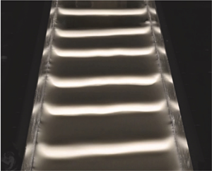
Figure 2. Experiments at high $\phi$ to characterize the Oobleck waves. (a) Sketch of the set-up used for $\phi >\phi _{DST}$, and a typical image of Oobleck waves ($\phi =0.45$, $\theta =10^\circ$, $Re\simeq 1.14\simeq 0.2\,Re_{Kap}$). (b) Image of the flow surface intersected by the laser sheet (same conditions as in a). (c) Reynolds number of the flow and amplitude of the perturbation $\Delta h_1$ and $\Delta h_2$ (same conditions as in a). The black dashed line indicates the instability threshold $Re_c$. (d) Normalized wave amplitude $\Delta h/h_0$ as a function of $x$ (same $\phi$ and $\theta$, $Re/Re_c=1.05$). The growth rate is measured over the region highlighted in blue.

For both protocols (above and below $\phi _{DST}$), we have verified that the same instability criteria are obtained from successive steady-state measurements at various constant flow rates. For each volume fraction investigated, experiments are repeated at least four times, and for each repetition, a new, freshly prepared, suspension is used to avoid starch aging or evaporation issues.

3.1. Base flow

We compute, first, the base flow, i.e. the steady uniform flow of a shear-thickening suspension, with volume fraction $\phi$, density $\rho$, and thickness $h_0$, down a plane with slope $\theta$. The base state will be denoted by the subscript $0$. For a layer with a stress-free surface, the momentum balance imposes that the shear stress $\tau _0$ increases linearly with the depth $h_0-z$, according to

(3.1)\begin{equation} \tau_0 (z) = \rho g (h_0-z) \sin \theta. \end{equation}

On the other hand, the shear stress is related to the shear rate by

(3.2)\begin{equation} \tau_0 (z) = \eta (\phi,z)\,\frac{\mathrm{d} u_0 (z)}{\mathrm{d} z}, \end{equation}

with $u_0 (z)$ the suspension velocity parallel to the plane, and $\eta (\phi,z)$ the suspension viscosity, which is generally not uniform. Combining (3.1) with (3.2) yields the velocity profile in terms of the reduced variable $\tau _0$:

(3.3)\begin{equation} u_0 (\tau_0) = \frac{1}{\rho g \sin \theta} \int_{\tau_0} ^{\tau_{b,0}} \frac{\tau '}{\eta(\phi,\tau')} \,\mathrm{d}\tau', \end{equation}

where $\tau _{b,0} \equiv \tau _0(z=0)=\rho g h_0 \sin \theta$ is the basal shear stress. Finally, the viscosity is given by the Wyart–Cates expression

(3.4)\begin{equation} \eta (\phi,\tau) = \eta_s \left[ \phi_0\,(1-\mathrm{e}^{-\tau^\ast{/}\tau}) +\phi_1\,\mathrm{e}^{-\tau^\ast{/}\tau} - \phi \right]^{-2}, \end{equation}

where $\eta _s$, $\tau ^\ast$, $\phi _0$ and $\phi _1$ are the rheological parameters introduced in § 2.1.

Figure 3 shows the base flow velocity profile obtained by integrating (3.3) numerically using (3.4), for volume fractions between 0.30 and 0.48. For low $\phi$, the velocity profile is semi-parabolic, as expected for a Newtonian fluid. For increasing $\phi$, the concavity of the profile reverses, which reflects the increase in the suspension viscosity at the bottom of the layer where the stress is the largest. The flowing region even localizes close to the free surface when the suspension jams beneath, i.e. when the basal stress reaches

(3.5)\begin{equation} \tau_{b,SJ} = \frac{\tau^\ast}{\ln\left(\dfrac{\phi_0-\phi_1}{\phi_0-\phi}\right)}. \end{equation}

Note that the vertical gradient of shear is expected to drive particle migration from the bottom to the top of the layer, which in turn should slightly modify the velocity profile (Carpen & Brady Reference Carpen and Brady2002; Dhas & Roy Reference Dhas and Roy2022). For simplicity, we do not consider this coupling between flow and volume fraction variation, which is not essential to account for the instabilities studied here.

Figure 3. (a) Sketch of the notations. (b) Velocity profiles of the base flow for the Wyart–Cates rheology with the parameters obtained from figure 1(b) and for various volume fractions ($\tau _{b,0}/\tau ^\ast =2$).

In the following analysis, we will use depth-averaged quantities and restrict the calculations to $\tau _{b,0}<\tau _{b,SJ}$, which does not affect the flow stability prediction (see figures 7b and 9c). From (3.3), the depth-averaged velocity of the base flow, $\bar {u}_0= ({1}/{h_0}) \int _0 ^{h_0} u_0(z) \, \mathrm {d} z =({1}/{\tau _{b,0}}) \int _0 ^{\tau _{b,0}} u_0(\tau )\,\mathrm {d}\tau$, is given by

(3.6)\begin{equation} \bar{u}_0 = \frac{h_0}{\tau_{b,0}^2} \int_0 ^{\tau_{b,0}} \int_{\tau} ^{\tau_{b,0}} \frac{\tau'}{\eta(\phi,\tau')} \,\mathrm{d} \tau'\,\mathrm{d}\tau. \end{equation}

This expression can be recast into a formal effective rheological law relating the basal stress $\tau _{b,0}$ to the effective shear rate $\bar {u}_0/h_0$, as

(3.7)\begin{equation} \frac{\bar{u}_0}{h_0} = \frac{\tau_{b,0}}{3\eta(\phi,\tau_{b,0})}\,\mathcal{G} (\phi,\tau_{b,0}), \end{equation}

where the function $\mathcal {G}$ is defined as

(3.8)\begin{equation} \mathcal{G} (\phi,\tau_b)= \frac{3\eta(\phi,\tau_b)}{\tau_b^3} \int_0 ^{\tau_b} \int_{\tau}^{\tau_b} \frac{\tau'}{\eta(\phi,\tau')} \,\mathrm{d}\tau'\,\mathrm{d}\tau. \end{equation}

For a Newtonian fluid with a uniform viscosity, $\mathcal {G}=1$. One recovers the basal stress relation for a steady uniform Newtonian flow, $\tau _{b,0}=3\eta \bar {u}_0/h_0$, where the factor 3 is a signature of the semi-parabolic velocity profile. For the Wyart–Cates shear-thickening law (3.4), $\mathcal {G}$ is no longer constant and depends on both the volume fraction $\phi$ and the relative basal stress $\tau _{b,0}/\tau ^\ast$.

Finally, the Reynolds number of the base flow is given by

(3.9)\begin{equation} Re = \frac{3\bar{u}_0^2}{gh_0\sin \theta}=\frac{\tau_{b,0}^3\,\mathcal{G}(\phi,\tau_{b,0})^2}{3\,\eta (\phi, \tau_{b,0})^2\rho g^2 \sin^2 \theta}. \end{equation}

The latter depends on three of the four main dimensionless parameters of the problem, namely, the Reynolds number based on the suspending liquid viscosity, $Re_s=\tau _{b,0}^3/(3\eta _s^2\rho g^2 \sin ^2 \theta )$, the volume fraction $\phi$, and the magnitude of the basal shear stress relative to the repulsive stress, $\tau _{b,0}/\tau ^\ast$, two of which are controlled by the flow thickness $h_0$. The fourth parameter is the inclination angle $\theta$.

The base state flow rule (3.7)–(3.8) summarizes the rheological behaviour of the suspension flow. It will be used in the following to study stability.

3.2. Depth-averaged equations

To study flow stability, we take advantage of the long nature of the observed waves, whose wavelength (${\sim }10$ cm) is much larger than the layer thickness ($h_0 \lesssim 1\,$cm). In this long wave limit, the vertical momentum balance implies that the pressure distribution is hydrostatic to the lowest order, and that horizontal viscous stress gradients can be neglected. Integrating the mass and horizontal momentum equations across the flow, for an incompressible medium, yields the depth-averaged, or Saint-Venant, equations

(3.10)$$\begin{gather} \frac{\partial h}{\partial t} + \frac{\partial h \bar{u}}{\partial x} = 0, \end{gather}$$

(3.11)$$\begin{gather}\rho \left( \frac{\partial h \bar{u}}{\partial t} + \frac{ \partial h \overline{u^2}}{\partial x}\right) = \rho g h \sin \theta - \tau_b - \rho g h \cos \theta\,\frac{\partial h}{\partial x}, \end{gather}$$

where $h(x,t)$ is the flow thickness, $\bar {u}(x,t)=(1/h)\int _0^h u(x,z,t) \,\mathrm {d}z$ is the depth-averaged velocity, $\overline {u^2}=(1/h)\int _0^h u^2(x,z,t) \,\mathrm {d}z$ is the averaged square velocity, and $u(x,z,t)$ is the parallel velocity component. The right-hand-side terms in (3.11) correspond to the gravity term, the basal shear stress, and the resultant of the horizontal gradient of hydrostatic pressure, respectively. To derive the last term, the normal stress tensor of the fluid is assumed isotropic at the lowest order.

To solve the system, closure relations are required for the basal stress $\tau _b$ and momentum flux term $\overline {u^2}$. Following a common approach in roll-wave studies (Kapitza & Kapitza Reference Kapitza and Kapitza1948; Trowbridge Reference Trowbridge1987; Ng & Mei Reference Ng and Mei1994; Forterre & Pouliquen Reference Forterre and Pouliquen2003), we assume that the base state flow rule (3.7)–(3.8), derived for a steady uniform flow, remains valid for an unsteady, non-uniform flow in the long-wavelength limit, which implies

(3.12)\begin{equation} \frac{\bar{u}}{h} = \frac{\tau_b}{3\eta(\phi,\tau_b)}\,\mathcal{G} (\phi,\tau_b)\equiv \dot{\gamma}(\tau_b). \end{equation}

Similarly, we rewrite the momentum flux term as $\overline {u^2}=\alpha \bar {u}^2$, and assume that the factor $\alpha$, which is set by the shape of the velocity profile, is constant and equal to the base state value. From (3.3), we obtain

(3.13)\begin{equation} \alpha = \dfrac{\tau_{b,0}\displaystyle\int_0 ^{\tau_{b,0}} \left(\displaystyle\int_{\tau}^{\tau_{b,0}} \dfrac{\tau'}{\eta(\phi,\tau')} \,\mathrm{d} \tau' \right)^2 \,\mathrm{d} \tau}{\left(\displaystyle\int_0 ^{\tau_{b,0}} \displaystyle\int_{\tau} ^{\tau_{b,0}} \dfrac{\tau'}{\eta(\phi,\tau')} \,\mathrm{d} \tau' \,\mathrm{d} \tau \right)^2 }. \end{equation}

For a Newtonian fluid (uniform viscosity), $\alpha =6/5$. This value increases as the flow localizes closer and closer beneath the surface. We will see that the instability threshold can be shifted significantly by the value of $\alpha$ at large volume fractions.

3.3. Linearization

To analyse the linear stability of the base state flow we non-dimensionalize equations using $\tilde {h}=h/h_0$, $\tilde {x}=x/h_0$, $\tilde {u}=\bar {u}/\bar {u}_0$, $\tilde {t}=t \, \bar {u}_0/h_0$, $\tilde {\tau }_b=\tau _b/\tau _{b,0}$ and $\tilde {\dot {\gamma }}=\dot {\gamma }h_0/\bar {u}_0$. The conservation equations and flow rule (3.10)–(3.12) become

(3.14)$$\begin{gather} \frac{\partial \tilde{h}}{\partial \tilde{t}} + \frac{\partial \tilde{h} \tilde{u}}{\partial \tilde{x}} = 0, \end{gather}$$

(3.15)$$\begin{gather}\frac{Re}{3} \left( \frac{\partial\tilde{h} \tilde{u}}{\partial \tilde{t}} + \alpha\,\frac{\partial \tilde{h} \tilde{u}^2}{\partial \tilde{x}}\right) = \tilde{h} - \tilde{\tau}_b - \frac{\tilde{h}}{\tan \theta}\,\frac{\partial \tilde{h}}{\partial \tilde{x}}, \end{gather}$$

(3.16)$$\begin{gather}\frac{\tilde{u}}{\tilde{h}} = \tilde{\dot{\gamma}}(\tilde{\tau}_b), \end{gather}$$

where $Re$ is given by (3.9).

Considering a small perturbation of the base flow, $\tilde {h}=1+h_1$, $\tilde {u}=1+ u_1$, $\tilde {\tau }_b=1+ \tau _1$, with $|h_1|, |u_1|, |\tau _1| \ll 1$, (3.14)–(3.16) become, at the lowest order,

(3.17)$$\begin{gather} \frac{\partial h_1}{\partial \tilde{t}} + \frac{\partial h_1}{\partial \tilde{x}} + \frac{\partial u_1}{\partial \tilde{x}} = 0, \end{gather}$$

(3.18)$$\begin{gather}\frac{Re}{3} \left( \frac{\partial u_1}{\partial \tilde{t}} + ( \alpha -1)\,\frac{\partial h_1}{\partial \tilde{x}}+ (2 \alpha -1)\,\frac{\partial u_1}{\partial \tilde{x}}\right) = h_1 - \tau_1 - \frac{1}{\tan \theta}\,\frac{\partial h_1}{\partial \tilde{x}}, \end{gather}$$

(3.19)$$\begin{gather}u_1-h_1=A\tau_1, \end{gather}$$

where $A$ is defined as

(3.20)\begin{equation} A \equiv \left( \frac{\mathrm{d} \tilde{\dot{\gamma}}}{{\mathrm{d} \tilde{\tau}_b}} \right)_{\tilde{\tau}_b = 1}=\frac{\tau_{b,0} h_0}{\bar{u}_0} \left( \frac{\mathrm{d} \dot{\gamma}}{\mathrm{d} \tau_b} \right)_{\tau_b=\tau_{b,0}}= \frac{3}{\mathcal{G} (\phi,\tau_{b,0})} -2, \end{equation}

and use has been made of the identity

(3.21)\begin{equation} \frac{\mathrm{d}}{\mathrm{d}\tau}\left(\int_0^{\tau} \int_{\tau'}^{\tau} \frac{\tau''}{\eta(\phi,\tau'')} \,\mathrm{d}\tau''\,\mathrm{d}\tau'\right) = \frac{\tau^2}{\eta(\phi,\tau)}. \end{equation}

The parameter $A$ represents the dimensionless inverse slope of the flow rule between the effective shear rate $\tilde {u}/h$ and the basal stress $\tilde {\tau }_b$. For a shear-thickening suspension following the Wyart–Cates flow rule, $A$ depends on $\phi$ and $\tau _{b,0}/\tau ^\ast$. It is equal to 1 for a Newtonian flow, and is negative for DST.

Overall, the linearized system (3.17)–(3.19) involves four dimensionless parameters, $\theta$, $Re$, $\alpha$ and $A$ (which are alternatives to those listed above, namely $\theta$, $Re_s$, $\tau _{b,0}/\tau ^\ast$ and $\phi$).

3.4. Modes and stability diagram

The system (3.17)–(3.19) is solved for a normal mode $h_1=H \exp ({{\rm i}(\tilde {k}\tilde {x} - \tilde {\omega }\tilde {t})})$, $u_1 = U \exp ({{\rm i}(\tilde {k}\tilde {x} - \tilde {\omega }\tilde {t})})$, with dimensionless wavenumber $\tilde {k}$ and dimensionless pulsation $\tilde {\omega }$. A non-trivial solution exists only if

(3.22)\begin{equation} {\rm det} \left( \begin{array}{cc} {\rm i} (\tilde{k}- \tilde{\omega}) & {\rm i}\tilde{k} \\ \dfrac{{\rm i}}{\tan \theta}\,\tilde{k} + \dfrac{Re}{3}\,(\alpha-1) {\rm i} \tilde{k} - \left(1+\dfrac{1}{A} \right) & \dfrac{Re}{3}\,({\rm i} \tilde{k} (2 \alpha -1 ) - {\rm i} \tilde{\omega}) + \dfrac{1}{A}\end{array} \right)= 0 , \end{equation}

which provides the dispersion relation

(3.23)\begin{equation} -\frac{Re}{3}\,\tilde{\omega} ^2 + \left( \frac{2 \, Re}{3}\,\alpha \tilde{k} - \frac{{\rm i}}{ A} \right) \tilde{\omega} + \left(\frac{1}{\tan \theta} -\frac{ Re \, \alpha}{3} \right)\tilde{k}^2 + \left( 1 + \frac{2}{A} \right) {\rm i} \tilde{k} = 0. \end{equation}

We conduct the temporal stability analysis with $\tilde {k}$ real and $\tilde {\omega }$ complex. Equation (3.23) is of order 2 in $\omega$ and has two branches. Each of these may actually embed different instabilities depending on the point of the phase space considered. To get insight into the physical meaning and stability of the branches, it is instructive to study their behaviour at low $\tilde {k}$, before giving the exact solutions. The structure of the dispersion relation ensures that the growth rate $\tilde {\sigma }=\mathrm {Im}[\tilde {\omega }(\tilde {k})]$ is monotonic and does not change sign with $\tilde {k}$, which means that the stability criterion at low $\tilde {k}$ is valid for all wavenumbers. Expanding the pulsation as $\tilde {\omega }= ia_0+c\tilde {k}+ia_2 \tilde {k}^2$ in the dispersion relation (3.23) gives the following two solutions at the lowest order in $\tilde {k}$:

(3.24)$$\begin{gather} \tilde{\omega}_1 \simeq (2+A)\tilde{k} + {\rm i} A \left[ \frac{Re}{3} \left[(2+A) (2+A-2\alpha) + \alpha \right]- \frac{1}{\tan \theta} \right]\tilde{k}^2, \end{gather}$$

(3.25)$$\begin{gather}\tilde{\omega}_{2} \simeq ( 2 \alpha - 2 - A ) \tilde{k} -{\rm i}\,\frac{3}{A\, Re}. \end{gather}$$

The first branch, $\tilde {\omega }_1(\tilde {k})$, is the ‘kinematic’ branch, since its wave speed in the long wave limit ($\tilde {k}\to 0$), $\tilde {c}_1=\mathrm {Re} (\tilde {\omega }_1) /\tilde {k} = 2 +A$, is that of kinematic waves, i.e. the slender small-amplitude waves that propagate at the speed $c_{kin}= (\mathrm {d}q/\mathrm {d}h)_0=\bar {u}_0 + h_0(\mathrm {d}\bar {u}/\mathrm {d}h)_0$, obtained by combining the steady flow rule $\bar {u}(h)$ with the mass equation (3.10) (Whitham Reference Whitham2011). Indeed, $c_{kin}$ can be expressed in terms of $A$ by noting that $\bar {u}(h)$ satisfies the force balance $\tau _b[\bar {u}(h)/h] = \rho g h\sin \theta$, in the base state. Differentiating with respect to $h$ and making use of the definition of $A$ in (3.20), one recovers $\tilde {c}_{kin} = 1+(h_0/\bar {u}_0)(\mathrm {d}\bar {u}/\mathrm {d}h)_0 = 2+A$.

The kinematic branch $\tilde {\omega }_1(\tilde {k})$ is unstable when the growth rate $\tilde {\sigma }_1\equiv \mathrm {Im}(\tilde {\omega }_1)$ is positive. Depending on the sign of $A$, two cases must be considered, which will be shown to concern two different instabilities. For $A>0$, i.e. when the effective rheology (3.12) is monotonic, the kinematic branch is unstable for large Reynolds numbers

(3.26)\begin{equation} Re > Re_{Kap} = \frac{3}{ \left[ (2+A)(2+A-2\alpha) +\alpha \right] \tan \theta}, \end{equation}

which extends the classical inertial Kapitza instability criteria to the shear-thickening rheology. In the Kapitza regime ($A>0$), inertia introduces a lag, which tends to amplify kinematic waves, while gravity tends to spread and stabilize them. The instability arises when the speed of kinematic waves is larger than the speed of gravity waves (Whitham Reference Whitham2011). For a Newtonian fluid ($A=1$ and $\alpha =6/5$), the threshold of the Kapitza instability predicted by (3.26) is $1/ \tan \theta$, which slightly overestimates the exact prediction $Re_{Kap, Newt} =(5/6)\tan \theta$ obtained from a rigorous long wave expansion of the Navier–Stokes equations (Benjamin Reference Benjamin1957; Yih Reference Yih1963). This well-documented discrepancy stems from assuming a fixed shape of the velocity profile. For a CST suspension ($0< A<1$), (3.26) predicts an increase in the critical Reynolds number relative to the Newtonian case. This is consistent with previous studies on power-law rheology fluids, which have shown that shear-thickening has a stabilizing effect on the flow (Hwang et al. Reference Hwang, Chen, Wang and Lin1994; Ng & Mei Reference Ng and Mei1994).

For $A<0$, i.e. when the effective flow rule (3.12) becomes negatively sloped, the stability condition is reversed. The kinematic branch is unstable for

(3.27)\begin{equation} Re < Re_{Kap} = \frac{3}{ \left[ (2+A)(2+A-2\alpha) +\alpha \right] \tan \theta}, \end{equation}

which means, surprisingly, that the kinematic branch is unstable at low Reynolds number, while inertia now has a stabilizing effect. This low Reynolds number instability, appearing for a negatively sloped flow rule ($A<0$), corresponds to the mechanism of formation of the Oobleck waves proposed by Darbois Texier et al. (Reference Darbois Texier, Lhuissier, Forterre and Metzger2020). Indeed, in the limit of vanishing inertia ($Re=0$), the dispersion relation (3.23) reduces to

(3.28)\begin{equation} \tilde{\omega}=(2+A)\tilde{k}-\frac{A}{\tan\theta}\,{\rm i}\tilde{k}^2, \end{equation}

or equivalently, in the spatio-temporal domain,

(3.29)\begin{equation} \frac{\partial h_1}{\partial t} + (2+A)\,\frac{\partial h_1}{\partial x} = \frac{A}{\tan \theta}\, \frac{\partial^2 h_1}{\partial x^2}. \end{equation}

One recognizes an advection–diffusion equation for the perturbative wave $h_1$, which predicts that waves propagate at the speed of kinematic waves $\tilde {c}_{kin}=2+A$, while diffusing with an effective diffusion coefficient $A/\tan \theta$. For $A<0$, waves anti-diffuse, i.e. grow during propagation. As discussed in Darbois Texier et al. (Reference Darbois Texier, Lhuissier, Forterre and Metzger2020), this instability can be understood, physically, as follows. In the absence of inertia, the balance of forces (3.11) between the gravity term, the basal stress and the pressure term implies that a locally positive (resp. negative) slope of the free surface causes a decrease (resp. increase) in the basal stress. Because of the negative slope of the flow rule ($A<0$), the basal stress variation induces anti-correlated velocity variations (positive upstream of a bump, and negative downstream), which amplify the initial perturbation.

The analysis above confirms that although they are both kinematic modes, the extended Kapitza instability ($A>0$) and Oobleck waves ($A<0$) are fundamentally different. For the latter, the destabilizing mechanism is non-inertial and inertia has only a stabilizing effect, which stabilizes high Reynolds number flow.

The second branch, $\tilde {\omega }_2(\tilde {k})$, with growth rate $\tilde {\sigma }_2=\mathrm {Im}(\tilde {\omega }_2)=-3{\rm i}/(A\,Re)$, is unstable only if $A<0$, regardless of Reynolds number. The condition on $A$ is the same as for Oobleck waves. However, the instability mechanism is, once again, fundamentally different. For the second branch, any perturbation is amplified when $A<0$, independently of whether or not a free surface is present, because inertia introduces a mismatch between the basal stress and the driving gravity force. The branch is not specific to free-surface flows and disappears in the strict absence of inertia ($Re=0$). For this reason, we call it the ‘inertial branch’.

The two critical curves, $A=0$ and $Re = Re_{Kap}$, lead to the stability diagram shown in figure 4, for an arbitrary plane inclination $\theta =10^\circ$. For the sake of simplicity, the predictions are plotted for a fixed value of $\alpha$ ($=1$, corresponding to a plug velocity profile). This simplification permits a two-dimensional representation, without altering the stability diagram, qualitatively. Note that the assumption $\alpha =1$ is made only in figure 4, while the rest of the analysis considers the exact value of $\alpha$ obtained from (3.13). In this case, the critical Reynolds number of the kinematic branch reduces to $Re_{Kap}=3/[(1+A)^2 \tan \theta ]$ (black solid line in figure 4a). As discussed above, the extended Kapitza instability develops for $A>0$ and $Re>Re_{Kap}$, and Oobleck waves for $A<0$ and $Re< Re_{Kap}$, whereas the inertial branch, shown in figure 4(b), is unstable for $A<0$ and $Re>0$.

Figure 4. Stability diagram $(Re,A)$ for (a) the kinematic branch, and (b) the inertial branch ($\theta =10^\circ$ and a plug flow profile, $\alpha =1$, is assumed for simplicity; see text). (a) Black line: Kapitza instability threshold ($Re=Re_{Kap}$). Red line: Oobleck waves instability threshold ($A=0$). (b) Dashed blue line: inertial branch instability threshold ($A=0$). (a,b) The green line indicates the Newtonian case ($A=1$). The coloured trajectories indicate the evolution of $Re$ and $A$ for various volume fractions and increasing flow rates (or basal stress $\tau _{b,0}$) ($\theta =10^\circ$, and the rheological parameters are those obtained from figure 1b). For most volume fractions above $\phi _{DST}$, the DST condition $Re = Re_{A=0}$ (i.e. $A=0$) is expected to be reached before (lower flow rate) the Kapitza instability onset ($Re = Re_{Kap})$.

To determine which criterion is reached first, and what instability is expected to be observed in practice, it is crucial to understand how $Re$ and $A$ vary in experiments given their coupled dependence on $\tau _{b,0}/\tau ^{\ast }$, $\theta$ and $\phi$. To this end, we display in figure 4 the trajectories followed by $A$ and $Re$ for an increasing flow rate (i.e. increasing $\tau _{b,0}/\tau ^{\ast }$ or flow thickness) and a fixed angle ($\theta =10^\circ$), which mimics the experimental protocol. The different trajectories correspond to different volume fractions, and the rheological parameters are those measured for the cornstarch suspensions (see § 2.1). Below $\phi _{DST}$, the trajectories only cross the $Re=Re_{Kap}$ critical line, since $A$ remains strictly positive for all flow rates. This means that the Kapitza instability is expected, provided that the flow rate is increased sufficiently. By contrast, above $\phi _{DST}$, one can, a priori, expect either the Kapitza instability or one of the two other instabilities (Oobleck wave and inertial branch), depending on which criterion ($A=0$ or $Re=Re_{Kap}$) is reached first when the flow rate is increased. This condition is given by the respective value of the two Reynolds numbers defined by

(3.30)\begin{equation} Re_{A=0} \equiv \frac{3}{4}\,\frac{\tau_{b,A=0}^3}{\rho[g\,\eta(\phi,\tau_{b,A=0})\sin\theta]^2}, \quad \text{with} \ \mathcal{G} (\phi,\tau_{b,A=0}) = \frac{3}{2}, \end{equation}

corresponding to the intersection of the iso-$\phi$ trajectory with the vertical axis $A=0$ (purple circle in figure 4), and

(3.31)\begin{equation} Re_{{Kap}, A=0} \equiv 3/[(4-3\alpha)\tan\theta] , \end{equation}

corresponding to the intersection between the Kapitza threshold and the vertical axis $A=0$ (black circle in figure 4). If $Re_{A=0} < Re_{{Kap}, A=0}$, as in figure 4, then the trajectory intersects the $A=0$ criterion first, meaning that Oobleck waves and inertial branches are expected to be observed first, for an increasing flow rate. In the opposite case ($Re_{A=0} > Re_{{Kap}, A=0}$), the trajectory first encounters the Kapitza threshold (with $A$ still positive), and the Kapitza instability is expected to develop first. The above condition between $Re_{A=0}$ and $Re_{{Kap}, A=0}$ involves $\phi$ non-trivially, the rheological parameters and the inclination angle $\theta$. However, as figure 4 shows, for cornstarch and provided that the plane remains far from the vertical ($\theta \ll 90^\circ$), the onset of DST ($A=0$) is reached before the Kapitza threshold ($Re_{Kap}$) for almost all volume fractions above $\phi _{DST}$.

In the following, the value of the Reynolds number when the first instability criterion is met for increasing flow rate and a fixed angle (i.e. following the iso-$\phi$ trajectories in figure 4) will be denoted by $Re_c$, in order to match the experimental definition. In practice, for our range of parameters (cornstarch rheology, plane far from vertical), $Re_c=Re_{Kap}$ for $\phi <\phi _{DST}$, and $Re_c=Re_{A=0}$ for $\phi >\phi _{DST}$.

3.5. Dispersion relation

The previous analysis has focused on the limit of vanishing $k$. We now solve the dispersion relation exactly for an arbitrary wavenumber. The two solutions of (3.23) are

(3.32)\begin{equation} \tilde{\omega}_{1, 2} = \dfrac{\dfrac{2\,Re}{3}\,\alpha \tilde{k} \pm \left(\dfrac{D+\sqrt{D^2+C^2}}{2}\right)^{1/2}}{\dfrac{2\,Re}{3}} + {\rm i}\,\dfrac{-\dfrac{1}{A} \pm \dfrac{C}{2} \left(\dfrac{2}{D+\sqrt{D^2+C^2}}\right)^{1/2}}{\dfrac{2\,Re}{3}}, \end{equation}

where $\pm$ stands for $+$ for the kinematic branch $\tilde {\omega }_{1}$, and $-$ for the inertial branch $\tilde {\omega }_{2}$, with

(3.33a,b)\begin{align} C = \dfrac{4\,Re}{3} \left(1 + \dfrac{2 - \alpha }{A}\right)\tilde{k} \quad {\rm and} \quad D =- \dfrac{1}{A^2}+\dfrac{4\,Re}{3}\left(\dfrac{Re}{3}\,\alpha(\alpha-1) + \dfrac{1}{\tan\theta}\right) \tilde{k}^2. \end{align}

Figures 5(a,b) present the growth rates for the two instabilities of the kinematic branch, namely, the Kapitza instability ($\phi = 0.33 < \phi _{DST}$, figure 5a) and the Oobleck wave instability ($\phi =0.45>\phi _{DST}$, figure 5b). The different colours stand for increasing values of $Re$ close to $Re_c$ (i.e. either $Re_{Kap}$ or $Re_{A=0}$). For both instabilities, the growth rate is null for $\tilde {k}=0$ and increases monotonically up to a plateau value at large $\tilde {k}$, which is the signature of a zero wavenumber instability. Interestingly, for a given wavenumber and distance to the threshold, the growth rate is several orders of magnitude larger for Oobleck waves than for the Kapitza instability (the vertical scale between the two panels differs by a factor $10^3$). Figures 5(c,d) present the wave speeds of the two instabilities for the same parameters. Close to the instability threshold, the wave speed depends only weakly on $\tilde {k}$. It drops from approximately 3 for the Kapitza instability, to 2 for Oobleck waves, in agreement with the long wave limit $2+ A$, since $A\simeq 1$ at the Kapitza threshold and $A=0$ at the Oobleck waves threshold.

Figure 5. Dispersion relations of the two instabilities of the kinematic branch ($\theta =10^\circ$). (a,c) Kapitza instability ($\phi =0.33$). (b,d) Oobleck waves instability ($\phi =0.45$). (a,b) Temporal growth rate $\mathrm {Im} (\tilde {\omega }_1)$. Note the highly different scales of the $y$-axis. (c,d) Wave speed $\tilde {c}_1$. (a–d) The yellow circles indicate the theoretical growth rates, for $Re=1.05\, Re_c$ and at the wavelength observed experimentally, which are compared with measurements in figure 8(b).

The growth rate of the inertial branch is shown in figures 6(a,b) for the same set of $\phi$ and $Re/Re_c$ as previously. We recover that the branch is unconditionally stable below $\phi _{DST}$, and unstable above $\phi _{DST}$ for Reynolds numbers larger than $Re_{A=0}$. By contrast with the kinematic branch, the growth rate is non-null at $\tilde {k}=0$ and actually diverges at the instability threshold $(A=0)$, where it changes sign, before decreasing with increasing $Re$ above the threshold. The corresponding wave speeds are presented in figures 6(c,d). For $\phi >\phi _{DST}$, the wave speed at threshold is lower than for the kinematic branch. Although the kinematic and inertial branches share the same criterion of stability for concentrated suspensions ($A=0$), the comparison between figures 5 and 6 suggests that they differ strongly in terms of growth and propagation speed. We address this point in the next section, where we compare predictions with experiments.

Figure 6. Dispersion relation of the inertial branch ($\theta =10^\circ$): (a,c) $\phi =0.33$, (b,d) $\phi =0.45$. (a,b) Temporal growth rate $\mathrm {Im} (\tilde {\omega }_2)$. (c,d) Wave speed $\tilde {c}_2$. The yellow circle indicates the theoretical growth rates, for $Re=1.05\,Re_c$ and at the wavelength observed experimentally, which are compared with measurements in figure 8(b).

4.1. Stability threshold

We compare, first, the stability criteria derived above with the wave onset conditions observed in experiments and detailled in Appendix A. Figure 7(a) presents $Re_c/Re_{Kap, Newt}$, i.e. the critical Reynolds number normalized by that for a Newtonian liquid ($Re_{Kap, Newt} = (5/6)/\tan \theta$; see § 3.4), as a function of $\phi$, whereas figure 7(b) reports the critical basal shear stress $\tau_c$, also versus $\phi$. The symbols represent the experimental measurements for various volume fractions. Each one is obtained by varying the flow rate at a fixed inclination of the plane (encoded by the shape of the symbol), as detailed in § 2. The solid lines represent the theoretical predictions for the same protocol, i.e. the critical Reynolds number $Re_c$ at which each iso-$\phi$ trajectory (see figure 4) reaches the $Re=Re_{Kap}$ or $Re=Re_{A=0}$ condition. The relative threshold $Re_c/Re_{Kap, Newt}$ is close to 1 at low volume fraction, where shear-thickening is mild, and increases with increasing $\phi$ to reach $\simeq 6$ at $\phi =0.41\simeq \phi _{DST}$. This illustrates the significant stabilization effect of CST in the Kapitza regime, in fair agreement with the evolution of $Re_{Kap}$ predicted by (3.26) (solid black line in figure 7a). Similarly, the steep increase in the critical stress $\tau_c$, which is observed experimentally close to $\phi =0.41$ (figure 7b), agrees with the expected divergence of the effective viscosity coefficient of the flow, $\mathrm {d}\tau _{b,0}/\mathrm {d}\dot {\gamma }\propto A^{-1}$, in $\phi _{DST}\simeq 0.41$. This confirms the Kapitza-like nature of the instability (destabilizing inertia versus stabilizing gravity) below $\phi _{DST}$.

Figure 7. Destabilization threshold: comparison with experiments. (a) Critical Reynolds number $Re_c$ normalized by the Newtonian Kapitza threshold $Re_{Kap, Newt}=(5/6)/\tan \theta$ versus volume fraction $\phi$. (b) Critical basal shear stress $\tau _c$ versus $\phi$. The symbols indicate measurements. Their shapes encode the inclination $\theta$: $\diamond$ $2^\circ$, $\triangledown$ $3^\circ$, $\triangleright$ $6^\circ$, $\triangleleft$ $9^\circ$, $\circ$ $10^\circ$, $\triangle$ $22^\circ$. The error bars indicate the standard deviation of the measurements at a given $\phi$. The lines represent the predictions for the different modes (as labelled above the graph), i.e. the critical Reynolds number at which each iso-$\phi$ trajectory (see figure 4) reaches the $Re=Re_{Kap}$ or $Re=Re_{A=0}$ condition. (The black line is interrupted above $\phi \simeq 0.42$ since no steady flow verifies $Re=Re_{Kap}$.) The shear-jamming limit corresponds to the value of the basal shear stress when the flow first jams at $z=0$ (see (3.5)). Inset: basal shear stress $\tau _{b,0}= \rho g h_0 \sin \theta$ versus mean shear rate $u_0/h_0$ for different volume fractions obtained from Wyart–Cates rheological laws (dashed lines) and from direct measurements on the inclined plane (solid lines). The red line and black crosses highlight the condition $\mathrm {d} \tau _b / \mathrm {d} \dot {\gamma }=0$ for both sets of curves.

Above $\phi _{DST}$, both the critical Reynolds number and the critical shear stress observed experimentally drop drastically, by up to two orders of magnitude, for $Re_c$, at $\phi =0.47$ (figure 7a). The drop in $Re_c$ is captured correctly by the theoretical prediction $Re_c = Re_{A=0}$ of (3.30), which, once again, applies to both Oobleck waves and the inertial waves instability, and does not permit us to distinguish between them. The agreement is also reasonable when the instability threshold is expressed in terms of $\tau_c$, although the prediction underestimates the measured value by approximately a factor 2 (figure 7b). To clarify this discrepancy, we note that the theoretical prediction relies on the value of the rheological parameters ($\eta _s$, $\phi _0$, $\phi _1$ and $\tau ^\ast$) as obtained from the cylindrical Couette rheometry (see § 2.1). In the inset of figure 7(b), we test these parameters more directly versus the inclined flow configuration by comparing the depth-averaged flow rule, $\tau _{b,0}$ versus $u_0/h_0$, that they predict, (3.7), with the one measured directly in the experiments on the incline. A significant difference is observed between the two flow rules, showing that the steady uniform flow down the incline is not well predicted from the rheological parameters obtained with the Couette rheometer. Such a difference has been reported previously in the case of non-shear-thickening suspensions (Bonnoit et al. Reference Bonnoit, Darnige, Clement and Lindner2010) and could arise from the modification of the velocity profile due to particle migration effects, which are not considered here (see § 3.1). Remarkably, however, when the expression for the critical shear stress $\tau_c$ is computed from the flow rule measured with the inclined plane (i.e. from the points $\mathrm {d}\dot {\gamma }/\mathrm {d} \tau _{b,0}=0$ highlighted by the black crosses in the inset of figure 7b), the agreement between the theoretical predictions and measurements becomes quantitative (crosses versus orange symbols in figure 7b). This suggests that the mild quantitative discrepancy between theory and experiments for $\tau _c$ stems not from a limitation of the linear stability analysis but rather from the calibration of the base flow itself.

The comparison above confirms that the onset of a negatively sloped flow rule ($A=0$) is, experimentally, the condition for flow stability above $\phi _{DST}$. However, it does not allow us to determine which of the kinematic branch or inertial branch is observed. To do so, the predictions for the growth rate and celerity of the waves, which differ between the two instability mechanisms, have to be compared with experiments.

4.2. Wave speed and growth rate

Figure 8(a) reports the wave speed, at the instability threshold, measured for various volume fractions. The ratio $c_c /u_c$ is almost constant around 3 at low volume fractions, decreases to approximately 2 between $\phi \simeq 0.37$ and $\phi =0.41\simeq \phi _{DST}$, and decreases further, a little below 2, for higher $\phi$. This behaviour agrees well with the prediction of the shear-thickening Kapitza regime expected below $\phi _{DST}$ (black solid line). Above $\phi _{DST}$, the measurements are found to match the prediction $\tilde {c}_c = 2$ for the kinematic branch better than the prediction $\tilde {c}_c =2 (\alpha -1) \simeq 0.6$ for the inertial branch, which suggests that the mechanism of the instability observed in experiments is that of Oobleck waves, rather than that of the inertial branch instability. This result is confirmed by a direct comparison between the measured wave speed and the speed of the kinematic waves $c_{kin}\equiv \mathrm {d} q/\mathrm {d} h_0$, as deduced from the experimental base flow measurements. As shown in the inset of figure 8(a), $c_c$ is fairly close to $c_{kin}$ over the whole range of volume fraction studied.

Figure 8. Wave speed and growth rate: comparison with experiments. (a) Wave speed $c_c$ normalized by the mean fluid velocity $u_c$ at the instability onset versus $\phi$. Inset: normalized wave velocity $c_c/u_c$ versus normalized speed of kinematic waves $c_{{kin}}/u_c$ at the onset. (b) Normalized spatial growth rate $\tilde {\sigma }$ versus $\phi$ for $Re/Re_c=1.05$.

The growth rates of the instability are compared in figure 8(b). The measurements are performed when the Reynolds number of the flow is 5 % above the observed critical value ($Re/Re_c=1.05$). The theory is computed for the wavelength observed experimentally at each $\phi$ (see figures 5 and 6). Here again, below $\phi _{DST}$, the growth rate is predicted correctly by the Kapitza instability accounting for continuous thickening (black solid line). Above $\phi _{DST}$, the prediction for the kinematic branch (red solid line) matches the measurements fairly well, whereas that for the inertial branch (blue dashed line) overestimates the observed growth rate by approximately two orders of magnitude.

The previous results indicate that including inertia in the depth-averaged analysis provides a fair description for both the shear-thickening Kapitza regime observed below $\phi _{DST}$ and the low Reynolds number Oobleck wave regime observed above $\phi _{DST}$. Nonetheless, one important question remains. Above $\phi _{DST}$, the inertial branch has the same instability condition as Oobleck waves, but since the former is expected to amplify two orders of magnitude faster (see figure 8b), why do we not observe, experimentally, the inertial mode rather than Oobleck waves?