


1. Introduction
Drug delivery in the human vasculature needs a great deal of understanding of the dispersion phenomenon in the Newtonian and non-Newtonian fluid flow in tubes. Under low shear rates, blood behaves as a non-Newtonian fluid, also in most of these situations, one needs to model it as a shear-thinning fluid. Solute dispersion in blood flow across vasculature has several physiological applications, likewise solute dispersion in non-Newtonian fluid flow has many applications in the chemical and ceramic industry. Pulsatile flows can be used for mimicking physiological systems and offers unique advantages over a steady flow, especially in microfluidic systems.
Taylor (Reference Taylor1953) initiated the theoretical and practical study of dispersion in fluid flow. Aris (Reference Aris1956) proposed the method of moments and explored the asymptotic behaviour in second-order moments around the mean, building on Taylor (Reference Taylor1953) theory. Gill & Sankarasubramanian (Reference Gill and Sankarasubramanian1970) and Barton (Reference Barton1983) investigated the solute dispersion in Newtonian fluid flow and presented for both the small and large time of injection of the solute. There have been more studies with mathematical treatment on solute distribution (Taylor Reference Taylor1953; Aris Reference Aris1956, Reference Aris1960; Gill & Sankarasubramanian Reference Gill and Sankarasubramanian1970; Gill, Sankarasubramanian & Taylor Reference Gill, Sankarasubramanian and Taylor1971; Sankarasubramanian & Gill Reference Sankarasubramanian and Gill1973; Chatwin Reference Chatwin1975; Joshi et al. Reference Joshi, Kamm, Drazen and Slutsky1983; Mazumder & Das Reference Mazumder and Das1992; Debnath et al. Reference Debnath, Jiang, Guan and Chen2022) considering the Newtonian fluid model (Aroesty & Gross Reference Aroesty and Gross1972; Sharp Reference Sharp1993; El Misiery Reference El Misiery2002; Nagarani, Sarojamma & Jayaraman Reference Nagarani, Sarojamma and Jayaraman2004; Boyd, Buick & Green Reference Boyd, Buick and Green2007; Rana & Murthy Reference Rana and Murthy2016a,Reference Rana and Murthyb,Reference Rana and Murthyc, Reference Rana and Murthy2017; Alsemiry, Sayed & Amin Reference Alsemiry, Sayed and Amin2022) and by considering non-Newtonian fluid modelling, for steady and unsteady flows in a straight and bent tubes, with and without wall absorption. Rana & Murthy (Reference Rana and Murthy2016a) reported research on the dispersion phenomenon of solute with boundary reaction/absorption in a pulsatile Casson fluid flow in a straight tube. The generalized dispersion model was used to investigate how the yield stress, the Womersley frequency parameter and the amplitude of the fluctuating pressure gradient component impact the solute dispersion. By using a similar methodology, Rana & Murthy (Reference Rana and Murthy2016b) provided the Gaussian solution for Herschel–Bulkley (H–B) non-Newtonian flow model and Rana & Murthy (Reference Rana and Murthy2017) investigated the two-phase (Casson–Newtonian) model. Bird et al. (Reference Bird, Curtiss, Armstrong and Hassager1987) discussed in detail the Carreau–Yasuda (C–Y) model. This model describes the fluid viscosity behaviour of the shear rate from low to high, as well as the fluid's shear-thinning nature. The solute dispersion process was explored by Rana & Murthy (Reference Rana and Murthy2016c) for non-pulsatile Carreau and C–Y fluid flow and computed three transport coefficients (exchange, convection and dispersion). Rana & Murthy (Reference Rana and Murthy2016c) explored the large-time action of the axial dispersion process in a steady non-Newtonian C–Y and Carreau fluid flow with the absorption of solute. By using a finite difference numerical technique, Das et al. (Reference Das, Sarifuddin, Rana and Kumar Mandal2022) observed solute dispersion in C–Y fluid flow. The effective axial diffusion coefficient of non-Newtonian fluids such as C–Y, Carreau, Casson, H–B, power-law and Bingham fluids (Nagarani et al. Reference Nagarani, Sarojamma and Jayaraman2004; Rana & Murthy Reference Rana and Murthy2016a,Reference Rana and Murthyb,Reference Rana and Murthyc, Reference Rana and Murthy2017) has been addressed. The C–Y fluid model has enough versatility to suit a large range of experimental apparent viscosity, which has been beneficial in hemodynamics. Alsemiry et al. (Reference Alsemiry, Sayed and Amin2022) studied the heat transfer properties of Carreau fluid within a catheterized artery, considering the Weissenberg number and the eccentric parameter as perturbation parameters.
Pulsating viscous flow superposed on the steady laminar motion of a Newtonian fluid in a circular pipe is investigated by Uchida (Reference Uchida1956), a phase lag of velocity variation from that of the pressure gradient is reported, and the distribution of the dissipation of energy that is associated with the pulsating viscous flow is estimated. The rate of mass transfer of a diffusing substance in an oscillatory motion of Newtonian fluid in a pipe has been investigated by Watson (Reference Watson1983), an analytical solution for the fluid velocity is obtained for both steady and pulsating pressure gradient. Pedley & Kamm (Reference Pedley and Kamm1988) investigated axial solute transport in a curved tube considering the unsteady flow that is influenced by the secondary flow. Sharp et al. (Reference Sharp, Kamm, Shapiro, Kimmel and Karniadakis1991) and Sharp, Carare & Martin (Reference Sharp, Carare and Martin2019) discussed flow and concentration behaviour in the viscous, unsteady and porous regimes based on the non-dimensional flow influencing parameters. This oscillatory flow with respect to a curved tube is first established and the Poiseuille scaling laws for transport are obtained by employing an order-of-magnitude analysis of the governing equations along the lines of Pedley & Kamm (Reference Pedley and Kamm1988).
Smith (Reference Smith1983) investigated longitudinal solute dispersion in a shear flow while accounting for the effect of boundary absorption. There is also a significant variation in the skewness of the solute dispersion curve. Wang & Chen (Reference Wang and Chen2017) investigated the Taylor dispersion in a laminar Newtonian flow considering absorption at the tube's surface, taking into account the first to fourth-order moments, and proposed analysis for the mean concentration distribution with the Hermite polynomials. The analysis described in Mehta, Merson & McCoy (Reference Mehta, Merson and McCoy1974), i.e. the zeroth to fourth-order moment expansion in terms of Hermite polynomial representation, was employed for this purpose, which was first proposed and applied in Kubin (Reference Kubin1965). Jiang & Chen (Reference Jiang and Chen2019) examined the transport of solute through a two-zone packed pipe with Newtonian fluid flow and explored the non-Gaussian distribution impacts of skewness and kurtosis for the steady case. Jiang & Chen (Reference Jiang and Chen2021) studied the transient dispersion of active particles in restricted planar steady Poiseuille flow. Furthermore, the drift, dispersivity and skewness were studied. Unsteady solute dispersion in a pulsatile H–B fluid flow in a tube has been reinvestigated by Singh & Murthy (Reference Singh and Murthy2022a) to examine the skewness and kurtosis on the concentration distribution using Aris’ method of moments considering Hermite polynomials. Yet another yield stress model, the Kuang and Luo (K–L) model, was also addressed very recently by Singh & Murthy (Reference Singh and Murthy2022b). These investigations bring in the accuracy in the estimation and measure the deflection and decrease in the axial mean concentration distribution of a solute in a tube. The velocity profiles of the pulsatile H–B fluid model and the K–L fluid have been calculated by using the regular perturbation technique but the non-yield stress C–Y fluid model requires extra treatment due to the existence of the Yasuda parameter  $a$. Many researchers tried to find the unsteady velocity profile of the C–Y fluid model but finally reduced their model into the steady case ( $e=0$) only (Rana & Murthy Reference Rana and Murthy2016c) or the Carreau fluid model ( $a=2$) (Alsemiry et al. Reference Alsemiry, Sayed and Amin2022). The present investigation is in pursuit of providing an approximate analytical solution for the velocity of the pulsatile C–Y fluid flow in the circular tube and investigating the solute dispersion considering the higher-order moments.
The present investigation examines the unsteady axial dispersion of a solute in the C–Y pulsatile fluid flow in a cylindrical tube, considering the impact of wall absorption. This study focuses on exploring the effect of skewness and kurtosis on solute dispersion in pulsatile non-yield stress fluid flow by using three different solution procedures: (i) Aris’ method of moments (including higher-order moments in § 2.2.1); (ii) Gill's generalized dispersion model (including higher-order coefficients in § 2.2.3); and (iii) a numerical procedure (using a new class of computationally explicit Runge–Kutta (CERK) method in Appendix A). Using Gill's method, Jiang & Chen (Reference Jiang and Chen2018) attempted to determine the non-Gaussianity in the solute dispersion in the steady Newtonian fluid flow in a circular pipe but the expressions for skewness and kurtosis are obtained using the moments generated by the Aris’ method of moments.
In this investigation, the solute dispersion in the unsteady C–Y fluid has been examined by considering the Aris’ method of moments by generating higher-order moments and expressions for the skewness and kurtosis. In addition, we have investigated the same problem using Gill's method and the expressions for skewness and kurtosis are derived independently. Also, a correspondence between the expressions for both skewness and kurtosis by using these two methods has been provided. Further to this, these results for the solute dispersion have been compared with the numerical solution obtained using a new class of CERK method. The flow and dispersion regimes are provided in § 3.3 for a better understanding of the solute dispersion. Firstly, the velocity profile for the pulsatile C–Y fluid is obtained using the Lagrange inversion theorem for small Womersley frequency parameter ( $\alpha <1$) and power law exponent ( $n<1$) for all other values of $\alpha$ and $n$, the velocity profile is obtained numerically. The velocity profiles for Carreau, the simplified Cross and the Newtonian model are obtained from this C–Y velocity profile. The increase in variance over time is not enough to provide detailed information about the concentration distribution. Skewness and kurtosis are also to be calculated for any approach to Gaussianity in the distribution. The impact of Yasuda parameter $a$, wall absorption parameter $\beta$, Weissenberg number $We$, power law exponent $n$, Womersley frequency parameter $\alpha$ and amplitude of fluctuating pressure gradient $e$ on convection coefficient $K_1(t)$, dispersion coefficient $K_2(t)$, skewness $K_3(t)$ and kurtosis $K_4(t)$, are investigated. Variations in two-dimensional concentration distribution $C$ and axial mean concentration $C_m$ are given in § 3.4. A comparative analysis between Newtonian and non-Newtonian fluid models is presented in § 3.1–3.4.
2. Mathematical formulation
Consider the pulsatile flow of C–Y fluid in a circular cylindrical tube or radius  $R$ as depicted in figure 1. The flow is unsteady, fully developed and axisymmetric. A solute slug is introduced into this stream at the initial time. The dispersion of a solute in the C–Y flow is examined. The solute is absorbed in the tube wall because of an irreversible first-order catalytic reaction. The rate of solute absorption is directly proportional to the solute concentration near the boundary. A dilute solution is adopted, which does not give rise to flux coupling (Sankarasubramanian & Gill Reference Sankarasubramanian and Gill1973; Rana & Murthy Reference Rana and Murthy2016c); such a coupling may arise in certain circumstances where the global transport process is driven by local gradients.

Figure 1. Schematic diagram of physical model.
2.1. Determination of the flow field
The C–Y fluid equation in one-dimensional shear flow with power-law exponent  $n$, time constant $\lambda$ and the Yasuda parameter $a$ is given by
 \begin{equation} \tau'={-} \left[\eta_\infty+(\eta_0-\eta_\infty) \left\{ 1+ \left(-\lambda \dfrac{\partial w'}{\partial r'}\right)^a\right\}^{(n-1)/ a}\right] \frac{\partial w'}{\partial r'}, \end{equation}
where,  $\tau '$ is the shear stress, $w'$ is the axial velocity, $r'$ is the radial direction and ${\partial w'}/{\partial r'}$ is the shear rate, $\eta _\infty$ is the infinite shear rate viscosity, $\eta _0$ is the zero shear rate viscosity, which gives the transition region (transition from zero shear rate region to power-law region). Equation (2.1) gives Carreau fluid at $a = 2$ and Newtonian fluid with viscosity $\eta _0$ at $n = 1$ or $\lambda = 0$.
The momentum equation is
 \begin{equation} \rho \frac{\partial w'}{\partial t'}={-}\frac{\partial p'}{\partial z'}-\frac{1}{r'} \frac{\partial (r'\tau')}{\partial r'}. \end{equation}
The initial and boundary conditions for (2.2) are
 \begin{equation} w'(R,t')=0,\quad \mbox{and}\quad \tau'(0,t') \quad \mbox{is finite.} \end{equation}
In the above,  $t'$ is the time.
The pulsatile pressure gradient at any axial location  $z'$ is
 \begin{equation} -\frac{\partial p'}{\partial z'}(t')=P_0+P_1 \sin(\omega t'), \end{equation}
where,  $P_0$ and $P_1$ are steady and fluctuating components of the pressure gradient, and $\omega$ represents the pressure pulsation frequency.
Consider the following non-dimensional variables:
 \begin{equation} \left.\begin{gathered} w=\frac{w'}{W_0},\quad r=\frac{r'}{R},\quad t= t' \omega,\quad \tau=\frac{\tau'}{\eta_0 (W_0/R)},\quad \eta =\frac{\eta_\infty}{\eta_0},\\ e=\frac{P_1}{P_0},\quad C=\frac{C'}{C_0},\quad z=\frac{D_m z'}{R^2 W_0}, \end{gathered}\right\} \end{equation}
where  $\eta$ is the viscosity ratio parameter, $D_m$ is the molecular diffusivity and $W_0$ is the characteristic velocity.
The shear stress (2.1) and momentum equation (2.2) reduces to a non-dimensional form as
 $$\begin{gather} \tau ={-} \left[\eta +(1-\eta ) \left\{ 1+ \left({-}We \frac{\partial w }{\partial r }\right)^a\right\}^{(n-1)/ a } \right] \frac{\partial w }{\partial r}, \end{gather}$$
 $$\begin{gather}\alpha^2 \frac{\partial w}{\partial t}=2p(t)-\frac{1}{r}\frac{\partial (r\tau)}{\partial r}. \end{gather}$$
 Here  $\alpha$ indicates the Womersley frequency parameter given by $\alpha = R/\sqrt {\nu /\omega }$ and $\nu$ denotes the kinematic viscosity coefficient. Also $We = \lambda W_0/R$ is the Weissenberg number. The pulsating pressure gradient is $p(t)=-({2}/{P_0})({\partial p'}/{\partial z'})=2[1+e \sin ( t)]$, where $e$ indicates the amplitude of fluctuating pressure gradient.
For the case when  $\alpha ^2<<1$ and $n\leq 1$, an analytical solution for the velocity profile has been obtained by using the perturbation technique. Here the parameter $\alpha ^2=\varepsilon$ is treated as the perturbation parameter. A new class of CERK method (Yadav et al. Reference Yadav, Ganta, Mahato, Rajpoot and Bhumkar2022) has been used to compute the velocity profile for all other values of $\alpha$ and $n$ and this procedure is explained in Appendix A.
The initial and boundary conditions for (2.6a) and (2.6b) are
 \begin{equation} w(r,0)=w_0(r,0),\quad w(1,t)=0\quad \mbox{and}\quad \tau(0,t) \quad \mbox{is finite}. \end{equation}
 In the above,  $w_0(r,0)$ is zeroth-order term of velocity $w(r,t)$ at $t=0$, which is defined in (2.8a,b) and its expression is given in (2.14) below.
Now the first-order series expansions for  $\tau (r,t)$ and $w(r,t)$ are written as
 \begin{gather} \tau(r,t)=\tau_0(r,t)+\varepsilon \tau_1(r,t)+ O(\varepsilon ^2)\quad \mbox{and}\quad w(r,t)=w_0(r,t)+\varepsilon w_1(r,t)+ O(\varepsilon ^2). \end{gather}
Using these expansions in (2.6a) and (2.6b), one obtains the constant and first-order  $\varepsilon$ equations along with their boundary conditions as
 $$\begin{gather} \frac{1}{r}\frac{\partial (r\tau_0)}{\partial r}- 2p(t)=0, \end{gather}$$
 $$\begin{gather}\tau_0(0,t) \quad \mbox{is finite}; \end{gather}$$
 $$\begin{gather} \tau_0 ={-} \left[ 1+\frac{(n-1)( 1- \eta )}{a} \left({-}We\frac{\partial w_0 }{\partial r }\right)^a\right] \frac{\partial w_0 }{\partial r }, \end{gather}$$
 $$\begin{gather}w_0(1,t)=0; \end{gather}$$
 $$\begin{gather} \frac{\partial w_0}{\partial t}={-}\frac{1}{r}\frac{\partial (r\tau_1)}{\partial r}, \end{gather}$$
 $$\begin{gather}\tau_1(0,t) \quad \mbox{is finite}; \end{gather}$$
 $$\begin{gather} \tau_1={-} \left[ 1+\dfrac{(a+1)(n-1)( 1- \eta )}{a} \left({-}We \frac{\partial w_0 }{\partial r }\right)^a \right]\frac{\partial w_1 }{\partial r }, \end{gather}$$
 $$\begin{gather}w_1(1,t)=0. \end{gather}$$
Following Aroesty & Gross (Reference Aroesty and Gross1972), the solution for  $\tau _0(r,t)$ is obtained from (2.9a), with boundary condition (2.9b) and it is given by
 \begin{equation} \tau_0(r,t)= r p(t). \end{equation}
 The velocity profile of the C–Y fluid model requires one extra treatment other than classical regular perturbation as seen in (2.8a,b), due to the existence of the Yasuda parameter  $a$ in (2.10a). The unsteady solution for all values of $a$ is obtained here using the Lagrange inversion theorem or Lagrange–Bürmann formula (Abramowitz & Stegun Reference Abramowitz and Stegun1964).
The solution  $w_0(r,t)$ is obtained from (2.10a) with the corresponding boundary condition (2.10b) by using Lagrange inversion theorem or Lagrange–Bürmann formula (details are given in Abramowitz & Stegun (Reference Abramowitz and Stegun1964)) and it is written as an infinite series as
 \begin{align} w_0(r,t)= \sum _{k=0}^\infty \frac{We^{a k} p(t)^{a k+1} }{({-}1)^{k+1} (a k+1) (a k+2)} {\binom{a k+k}{k}}\left(\frac{(n-1)(1- \eta ) }{a}\right)^k \left(r^{a k+2}-1\right). \end{align}
Using  $w_0(r,t)$ in (2.11a) with the boundary condition (2.11b), the first-order term of shear stress $\tau _1 (r,t)$ is obtained as
 \begin{align} \tau_1(r,t)=\sum _{k=0}^\infty \frac{We^{a k} p(t)^{a k}}{({-}1)^{k}(a k+2)} \frac{\partial p (t) }{\partial t} {\binom{a k+k}{k}} \left(\frac{(n-1)(1- \eta ) }{a}\right)^k \left(\frac{r^{a k+3}}{a k+4}-\frac{r}{2}\right). \end{align}
Using  $\tau _0(r,t)$, $w_0(r,t)$ and $\tau _1(r,t)$ in (2.12a) with the boundary condition (2.12b), the first-order velocity $w_1(r,t)$ is obtained and it is given by
 \begin{align} w_1(r,t) &={-}\frac{1}{32} \frac{\partial p (t) }{\partial t} (r^4-4 r^2+3 )- We^a\frac{(a+1)(n-1) ( 1-\eta )}{a} p(t)^a \frac{ \partial p (t) }{\partial t} \nonumber\\ &\quad \times \left[\frac{(r^{a+2}+r^2-2)}{4 (a+2)} -\frac{(a^2+6 a+16 ) }{8 (a+2) (a+4)^2}(r^{a+4}-1 ) \right] \nonumber\\ &\quad - We^{2a}\frac{(n-1)^2 ( 1-\eta )^2 }{a^2} ~ p(t)^{2 a} \frac{ \partial p (t) }{\partial t} \nonumber\\ &\quad \times\left[\frac{1}{(2 a+4)}\left\{\frac{(a+1)^2}{(a+2) (a+4)}+ \frac{(2 a+1) (a+1)}{8} +\frac{2 a+1}{4 (a+2)}\right\}(r^{2 a+4}-1 ) \right.\nonumber\\ &\quad \left. -\frac{ (2 a+1)}{8} (r^{2 a+2}-1 ) -\frac{(a\!+\!1)^2 }{2 (a\!+\!2)^2}(r^{a+2}-1 ) -\frac{(2 a+1)}{8} (r^2-1 ) \right]. \end{align}
The stress  $\tau (r,t)$ and velocity $w(r,t)$ have been computed using (2.8a,b).
2.2. Determination of the concentration field
The unsteady solute transport in the present physical configuration is governed by the initial boundary value partial differential equations given by
 \begin{equation} \frac{\partial C'}{\partial t'}+w'(r',t')\frac{\partial C'}{\partial z'}=D_m \left(\frac{1}{r'}\frac{\partial}{\partial r'} \left( r' \frac{\partial C'}{\partial r'}\right)+ \frac{\partial^2 C'}{\partial z'^2} \right), \end{equation}
 $$\begin{gather} C'(r',z',0)=\frac{M}{{\rm \pi} R^2} \delta(z'),\quad -D_m \frac{\partial C'}{\partial r'}(R,z',t')=kC'(R,z',t'), \end{gather}$$
 $$\begin{gather}\frac{\partial C'}{\partial r'}(0,z',t')=0,\quad C'(r',\infty,t')=0,\quad \frac{\partial C'}{\partial z'}(r',\infty,t')=0, \end{gather}$$
where  $\delta (z')$is a Dirac delta function and $k$ is the reaction rate constant.
Using (2.5a–h) the non-dimensional form of above equation is
 \begin{equation} \mathcal{P} ^2 \frac{\partial C}{\partial t}+w(r,t)\frac{\partial C}{\partial z}=\frac{1}{r} \frac{\partial}{\partial r} \left(r \frac{\partial C}{\partial r}\right)+\frac{1}{Pe^2} \frac{\partial^2 C}{\partial z^2}, \end{equation}
 $$\begin{gather} C(r,z,0)=\delta(z)/Pe,\quad \frac{\partial C}{\partial r}(1,z,t)={-}\beta C(1,z,t), \end{gather}$$
 $$\begin{gather}\frac{\partial C}{\partial r}(0,z,t)=0,\quad C(r,\infty,t)=0,\quad \frac{\partial C}{\partial z}(r,\infty,t)=0. \end{gather}$$
The Péclet number  $Pe$ is given by $Pe=RW_0/D_m$ and the oscillatory Péclet number $\mathcal {P}^2$ is given by $\mathcal {P}^2=\alpha ^2 Sc=R^2 \omega /D_m$ (Sharp et al. Reference Sharp, Carare and Martin2019). The Schmidt number $Sc$ is given by $Sc=\nu /D_m$ and the value of the Schmidt number is considered to be $O(10^3)$, which is consistent with those value for blood flow in arteries. The wall absorption parameter is represented by $\beta =kR/D_m$.
2.2.1. Aris’ method of moments for concentration distribution
Following the standard method of moments (Aris Reference Aris1956; Barton Reference Barton1983), define the  $n$th moment of concentration as
 \begin{equation} C_n(r,t)= \int_{-\infty}^{+\infty}z^n C(r,z,t)\,{\rm d} z. \end{equation}
Multiplying the diffusion equation (2.19) with  $z^n$ and integrate with respect to $z$ and using (2.21), the equations for determining the $C_n(r,t)$ are obtained as
 \begin{equation} \mathcal{P}^2 \frac{\partial C_n}{\partial t}- \frac{1}{r }\frac{\partial}{\partial r } \left( r \frac{\partial C_n}{\partial r }\right)=n w(r,t) C_{n-1}+\frac{1}{Pe^2} n(n-1) C_{n-2}, \end{equation}
where  $n=0,1,2,3,4,\ldots.$, with $C_{-1}$ and $C_{-2}$ set to zero.
Accordingly, the initial and boundary conditions given in (2.20a) are written as
 \begin{equation} C_n(r,0)= \frac{1}{Pe} \delta_{n0},\quad \frac{\partial C_n}{\partial r}( 0,t) =0,\quad \frac{\partial C_n}{\partial r}( 1,t)+\beta C_n( 1,t)=0. \end{equation}
The cross-sectional averaged  $n$th moment of solute distribution is given by
 \begin{equation} \langle C_n(t) \rangle= \int_{0}^{1}2 r C_n(r,t )\,{\rm d} r, \end{equation}
where  $\langle {\cdot } \rangle$ indicate the mean of cross-section. The $n$th central moment about the mean concentration distribution is written as
 \begin{equation} M_n(t)= \frac{\displaystyle\int_{0}^{1} \int_{-\infty}^{+\infty}2 r(z-\mu_g)^n C\,{\rm d} z\,{\rm d} r}{ \displaystyle\int_{0}^{1} \int_{-\infty}^{+\infty}2 r C\,{\rm d} z\,{\rm d} r}, \end{equation}
where
 \begin{equation} \mu_g= \frac{\displaystyle\int_{0}^{1} \int_{-\infty}^{+\infty}2 r z C \,{\rm d} z \,{\rm d} r}{\displaystyle\int_{0}^{1} \int_{-\infty}^{+\infty}2 r C\,{\rm d} z\,{\rm d} r}= \frac{\langle C_1 \rangle}{\langle C_0 \rangle}, \end{equation}
it represents the centroid,  $\langle C_0 \rangle$ is the dimensionless initial (or entire) mass of chemical species in the flow.
2.2.2. Estimation of  $C_n(r,t )$ and $K_n(t)$ for $n=0,1,2,3,4$


By taking  $n=0,1,2,3,4$ in (2.22) and (2.23a–c), the resulting homogeneous and non-homogeneous initial boundary value problems are solved using the eigenfunction expansion method suggested by Boyce & DiPrima (Reference Boyce and DiPrima2001). The eigenfunction expansion solutions of $C_n(r,t)$ for $n=0,1,2,3,4$ are given by (C1)–(C5) in Appendix B.
The mass of solute is exponentially decaying with time owing to absorption at the boundary (Dalal & Mazumder Reference Dalal and Mazumder1998), so the exchange coefficient  $K_0(t)$ may be written as
 \begin{equation} K_0(t)= \mathcal{P}^2 \frac{{\rm d}}{{\rm d} t} \left( \log \langle C_0 (t) \rangle \right) ={-} \frac{\displaystyle\sum_{n=1}^{\infty} A_n^{'}\mu_n {\rm J}_1(\mu_n) \exp({-\mu_n^2 t /\mathcal{P}^2})}{\displaystyle\sum_{n=1}^{\infty} (A_n^{'} {\rm J}_1(\mu_n)/\mu_n) \exp({-\mu_n^2 t/\mathcal{P}^2})}. \end{equation}
 The rate with which the centre of mass proceeds is equivalent to the fluid convection (Dalal & Mazumder Reference Dalal and Mazumder1998), so the convection coefficient  $K_1(t)$ is obtained from
 \begin{equation} K_1(t)={-} \mathcal{P} ^2 \frac{{\rm d}\mu_g}{{\rm d} t}={-}\mathcal{P} ^2 \frac{{\rm d}}{{\rm d} t}\left(\frac{\langle C_1 \rangle}{\langle C_0 \rangle}\right). \end{equation}
Here  $M_2$ is the second-order central moment that represents the variance of solute concentration. According to Aris (Reference Aris1956), the rate of change of variance is proportional to the sum of the molecular diffusion coefficient along the axial direction and apparent dispersion coefficient in the radial direction. As the axial diffusion is small in comparison with the lateral diffusion, the apparent dispersion coefficient $K_2(t)$ can be written as
 \begin{align} K_2(t) &=\frac{\mathcal{P} ^2 }{2}\frac{{\rm d} M_2}{{\rm d} t} = \frac{\mathcal{P} ^2 }{2}\frac{{\rm d}}{{\rm d} t} \left(\frac{\langle C_2 \rangle}{\langle C_0 \rangle}-\mu_g^2 \right)= \frac{F_{1}(t) }{F_3(t)} +\frac{F_2 F_4(t)}{F_3(t)^2} \nonumber\\ &\quad +2\frac{F_5(t) F_6(t)}{F_3(t)^2} +2\frac{F_5(t)^2 F_4(t) }{F_3(t)^3}. \end{align}
The skewness  $K_3(t)$ measures the degree of symmetry of the axial concentration distribution (Dalal & Mazumder Reference Dalal and Mazumder1998), and it is represented by
 \begin{equation} K_3(t) = \frac{M_3}{M_2^{3/2}} = \frac{\dfrac{\langle C_3 \rangle}{\langle C_0 \rangle}-3\mu_g M_2-\mu_g^3}{M_2^{3/2}}. \end{equation}
Also, the kurtosis  $K_4(t)$ measures the peak of the concentration distribution (Dalal & Mazumder Reference Dalal and Mazumder1998) and it is represented by
 \begin{equation} K_4(t) = \frac{M_4}{M_2^{ 2}}-3,\quad \mbox{where}\quad M_4= \frac{\langle C_4 \rangle}{\langle C_0 \rangle}-4\mu_g M_3-6 \mu_g^2 M_2-\mu_g^4. \end{equation}
In the above equations,  $\mu _n$ are roots of $\mu _n \textrm {J}_1(\mu _n)=\beta \textrm {J}_0(\mu _n)$, $n=0,1,2,3,\ldots 10$ and these are plotted in figure 2 (the intersection points of $\mu _n \textrm {J}_1(\mu _n)$ and $\beta \textrm {J}_0(\mu _n)$ are $\mu _n$). The initial guess value of the first root has been considered from this figure. By using the Newton–Raphson method all other roots are obtained. $A_n^{'},\ A_m^{''}$, $B_{1}$ to $B_4$, $X_1$ to $X_4$, $F_{1}$ to $F_{6}$ is given in Appendix D with Bessel functions of first kind of order zero $\textrm {J}_0$ and one $\textrm {J}_1$.

Figure 2. Solutions for the transcendental equation  $\mu _n \textrm {J}_1(\mu _n)=\beta \textrm {J}_0(\mu _n)$. The intersection points are the locations of root $\mu _n$: (a) $\beta =0.01$ and (b) $\beta =100$.
2.2.3. Gill's generalized dispersion method for concentration distribution
The convective diffusion equation (2.19) is solved using Gill's generalized dispersion method in this section along with the initial and boundary conditions. Following Gill & Sankarasubramanian (Reference Gill and Sankarasubramanian1970), the solute concentration  $C(t, z, r)$ is expanded in an infinite series as
 \begin{equation} C(t, z, r) = \sum_{n=0}^{\infty} f_n ( r,t) \frac{\partial^n C_m( z,t)}{\partial z^n}, \end{equation}
where the mean concentration  $C_m( z,t)$ is defined by
 \begin{equation} C_m( z,t)= \int_{0}^{1}2 r C (r,z,t)\,{\rm d} r. \end{equation}
Substituting the expansion (2.32) into the governing equation (2.19), we obtain the important Taylor–Gill expansion equation for  $C_m( z,t)$ as
 \begin{equation} \mathcal{P}^2 \frac{\partial C_m( z,t)}{\partial t} =\sum_{n=0}^{\infty} k_n (t) \frac{\partial^n C_m( z,t)}{\partial z^n}, \end{equation}
where the transport coefficients  $k_n,\ n=0,1,2,3,4$ are given by
 \begin{equation} k_n(t) =\frac{\delta_{n2}}{Pe^2}+ 2 \left.\frac{\partial f_n( r,t)}{\partial r}\right|_{r=1}- \int_{0}^{1} 2rw(r,t)f_{n-1}(r, t)\,{\rm d} r. \end{equation}
Here,  $k_0(t),\ k_1(t),\ k_2(t)$ are the exchange coefficient due to non-zero solute flux at the tube wall, convection coefficient due to the velocity of solute and dispersion coefficient due to the molecular diffusion and the velocity of the fluid, respectively (Rana & Murthy Reference Rana and Murthy2016a).
Substituting (2.34) and (2.32) into (2.19), and equating the coefficients of  ${\partial ^n C_m( z,t)}/{\partial z^n}\ (n=0,1,2,3,4)$, the set of differential equations for $f_n$ are obtained as
 \begin{equation} \mathcal{P}^2 \frac{\partial f_n}{\partial t}= \frac{1}{r } \frac{\partial}{\partial r } \left( r \frac{\partial f_n}{\partial r }\right)- w(r,t) f_{n-1}+ \frac{f_{n-2} }{Pe^2} - \sum_{i=0}^{\infty} k_i ( t) f_{n-i}. \end{equation}
Using (2.32) and (2.19) in the initial and boundary conditions (2.20a), the coefficients  $C_m$ and $f_n$ are expressed as
 $$\begin{gather} C_m(z,0)= \frac{\delta(z)}{Pe},\quad C_m( \infty,t)=0,\quad \frac{\partial C_m }{\partial z}( \infty,t)=0. \end{gather}$$
 $$\begin{gather}f_n(r,0)= \frac{\delta_{n0}}{Pe},\quad \frac{\partial f_n}{\partial r} (0,t) =0,\quad \frac{\partial f_n}{\partial r}( 1,t)+\beta f_n( 1,t)=0. \end{gather}$$
2.2.4. Estimation of $f_n(t, r)$ and $k_n(t)$


Equation (2.36) can be rewritten as
 \begin{equation} \mathcal{P}^2 \frac{\partial f_n}{\partial t}- \frac{1}{r }\frac{\partial}{\partial r} \left( r \frac{\partial f_n}{\partial r }\right)+ k_0 ( t) f_{n } ={-} \left[w(r,t) f_{n-1}-\frac{f_{n-2} }{Pe^2} + \sum_{i=1}^{\infty} k_i ( t) f_{n-i}\right]. \end{equation}
The solution of the above equation is
 \begin{equation} f_n(r,t)= \exp\left({-\left(\int_0^t k_0(s)\,{\rm d} s\right)/\mathcal{P}^2}\right) g_n(r,t), \end{equation}
where  $g_n(r,t)$ is the solution of the governing equation
 \begin{equation} \mathcal{P}^2 \frac{\partial g_n}{\partial t}- \frac{1}{r} \frac{\partial}{\partial r } \left( r \frac{\partial g_n}{\partial r }\right) ={-} \left[w(r,t) g_{n-1}-\frac{g_{n-2} }{Pe^2} + \sum_{i=1}^{\infty} k_i (t) g_{n-i} \right] . \end{equation}
The method of eigenfunction expansion is used to determine  $g_n(r,t)$ and $f_n(r,t)$ and it is given by
 $$\begin{gather} g_0(r,t)= \sum_{m=0}^{\infty} A_m^{'} {\rm J}_0(\mu_m r) \exp({-\mu_m^2 t/\mathcal{P}^2}), \end{gather}$$
 $$\begin{gather}f_0(r,t)= \exp\left({- \left(\int_0^t k_0(s)\,{\rm d} s\right)/\mathcal{P}^2}\right) \left[\sum_{m=0}^{\infty} A_m^{'} {\rm J}_0(\mu_m r) \exp({-\mu_m^2 t/\mathcal{P}^2})\right], \end{gather}$$
 $$\begin{gather} f_n(r,t) ={-} \exp\left({-\left(\int_0^t k_0(s)\,{\rm d} s\right)/\mathcal{P}^2}\right) \left[\sum_{m=0}^{\infty}A_m^{''^2}{\rm J}_0(\mu_m r) \right.\nonumber\\
\left.\times\int_0^t \left( \int_0^1 rF_n(r,s) {\rm J}_0(\mu_m r)\,{\rm d} r \right) \frac{\exp({- \mu_m ^2(s-t)/\mathcal{P} ^2})}{\mathcal{P}^2}{\rm d} s\right],\quad n\geq 1, \end{gather}$$
$$\begin{gather} f_n(r,t) ={-} \exp\left({-\left(\int_0^t k_0(s)\,{\rm d} s\right)/\mathcal{P}^2}\right) \left[\sum_{m=0}^{\infty}A_m^{''^2}{\rm J}_0(\mu_m r) \right.\nonumber\\
\left.\times\int_0^t \left( \int_0^1 rF_n(r,s) {\rm J}_0(\mu_m r)\,{\rm d} r \right) \frac{\exp({- \mu_m ^2(s-t)/\mathcal{P} ^2})}{\mathcal{P}^2}{\rm d} s\right],\quad n\geq 1, \end{gather}$$where,
 \begin{equation} F_n(r,t)= \left[w(r,t) g_{n-1}-\frac{g_{n-2} }{Pe^2} + \sum_{i=1}^{\infty} k_i ( t) g_{n-i}\right]. \end{equation}
Now using the mean concentration  $C_m(z,t)$ as defined in (2.33) into (2.32), we have
 \begin{equation} \int_0^1 r f_n(r,t)\,{\rm d} r = \frac{\delta_{n0}}{2}. \end{equation}
By using the above condition in (2.44), gives the solution of  $\int _0^t k_n(s)\,\textrm {d} s$ as
 $$\begin{gather} \exp\left({- \left(\int_0^t k_0(s)\,{\rm d} s\right)/\mathcal{P}^2}\right) = \frac{1}{\displaystyle\sum_{m=0}^{\infty} 2 A_m^{'} ({\rm J}_1(\mu_m )/\mu_m) \exp({-\mu_m^2 t/\mathcal{P} ^2 })}, \end{gather}$$
 $$\begin{gather}\int_0^t k_1(s)\,{\rm d} s ={-} \mathcal{P} ^2 \frac{Y_1(t)}{Y_0(t)}, \end{gather}$$
 $$\begin{gather}\int_0^t k_2(s)\,{\rm d} s = \mathcal{P} ^2 \frac{Y_2(t)Y_0(t)-Y_1(t)^2}{2 Y_0(t)^2}, \end{gather}$$
 $$\begin{gather}\int_0^t k_3(s)\,{\rm d} s = \mathcal{P}^2 \frac{Y_1(t)^3 - 3 Y_1(t)^3 + 3 Y_2(t)Y_1(t) Y_0(t) -Y_3 (t) Y_0(t)^2}{6 Y_0(t)^3}, \end{gather}$$
 $$\begin{gather}\int_0^t k_4(s)\,{\rm d} s =\mathcal{P}^2 \frac{ Y_4(t)Y_0(t)^3 +6 Y_0(t)Y_1(t)^2 Y_2(t) -4Y_0(t)^2 Y_1(t)Y_3(t) -3Y_1(t) ^4 }{24 Y_0(t)^4}, \end{gather}$$
where  $Y_0$ to $Y_4$ are given in Appendix C.
Since,  $K_0(t),\ K_1(t),\ K_2(t)$ are the exchange coefficient, convection coefficient and dispersion coefficient (same as $k_0(t),\ k_1(t), k_2(t)$). Thus, it can be written as
 \begin{equation} K_0(t)= k_0(t),\quad K_1(t)= k_1(t),\quad K_2(t)= k_2(t). \end{equation}
 Following Jiang & Chen (Reference Jiang and Chen2018), skewness  $K_3(t)$ and kurtosis $K_4(t)$ can be written in terms of coefficients $k_n(t)$ as
 \begin{equation} K_3(t)={-} \frac{3 \mathcal{P} \displaystyle\int_0^t k_3(s)\,{\rm d} s}{\sqrt{2} \displaystyle\left(\int_0^t k_2(s)\,{\rm d} s\right)^{3/2}},\quad K_4(t)= \frac{6 \mathcal{P} ^2 \displaystyle \int_0^t k_4(s)\,{\rm d} s}{\displaystyle\left(\int_0^t k_2(s)\,{\rm d} s\right)^{2}}. \end{equation}
 The effects of non-Gaussian distribution are captured by the higher-order dispersion model. Skewness and kurtosis can also measure how important higher-order coefficients are in comparison with second-order coefficients. Jiang & Chen (Reference Jiang and Chen2018) provided the relationship between  $k_n(t)$ and $M_n(t)$ as $k_n(t) =\mathcal {P} ^2 ({(-1)^n}/{n!}) ({\textrm {d} M_n}/{\textrm {d} t})$ for the steady Newtonian fluid. From the present analysis for the non-Newtonian model, we notice that $\int _0^t k_n(s)\,\textrm {d} s =({(-1)^n}/{n!}) \mathcal {P}^2 M_n$, which is the same as the above relation as given in Jiang & Chen (Reference Jiang and Chen2018) at $\mathcal {P} ^2=1$. This is evident from sets of equations given in (2.48)–(2.51) and (2.28)–(2.31). In figure 3, the expressions for $K_1(t),\ K_2(t),\ K_3(t)$ and $K_4(t)$ computed by using the Aris method of moments and Gill's method are shown for Newtonian and non-Newtonian fluids which are seen to agree up to higher-order precision.

Figure 3. Variation of (a) negative convection coefficient  $-K_1(t)$; (b) dispersion coefficient $K_2(t)$; (c) skewness coefficient $K_3(t)$; (d) kurtosis coefficient $K_4(t)$ by using Aris’ method of moments and Gill's generalized dispersion model (triangular marker) with time $t$ for different Newtonian and non-Newtonian fluids, when $\alpha = 0.5$, $\beta =0.01,\ Pe=1000, Sc=1000$ and $e=0.5$.
2.2.5. Axial mean concentration $C_m(z,t)$ and two-dimensional concentration $C(r,z,t)$


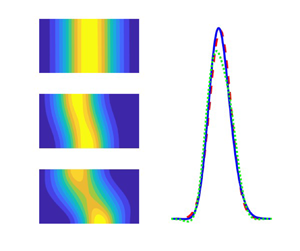
The axial mean concentration distribution is now approximated by applying fourth-order Hermite polynomials to describe non-Gaussian curves after the initial five concentration moments have been computed. It is obtained as
 \begin{equation} C_m(z,t)=\langle C_0(t) \rangle\,{\rm e}^{-\zeta^2} \sum_{n=0}^{\infty} a_n(t) H_n(\zeta(t)), \end{equation}
where,  $\zeta (t)= {(z-\mu _g(t))}/{\sqrt {2 M_2(t)} }$ and $H_0(\zeta ) =1$. The Hermite polynomials $H_i$ obey the recurrence relation
 \begin{equation} H_{i+1}(\zeta) =2 \zeta H_i(\zeta)-2 i H_{i-1}(\zeta),\quad i=0,1,2,3,\ldots. \end{equation}
 Also, the coefficients  $a_n(t)$ mentioned in (2.54) are given by
 \begin{align} a_0(t) =\frac{1}{ \sqrt{2 {\rm \pi}M_2(t)}},\quad a_1 = a_2=0,\quad a_3 (t)=\frac{\sqrt{2} a_0 K_3(t)}{24},\quad a_4(t)=\frac{a_0 K_4(t)}{96}. \end{align}
Now, the two-dimensional concentration distribution  $C(r,z,t)$ is calculated by Andersson & Berglin (Reference Andersson and Berglin1981) using $C_n(r,t)$ in the place of $\langle C_n(t) \rangle$ for moments $M_0, M_1, M_2, M_3, M_4$ and transport coefficients $K_0, K_1, K_2, K_3, K_4$.
3. Results and discussion
Most of the results are reported in this investigation considering three periods ( $3 T$), where $T=2 {\rm \pi}$. The physically realistic range of values of the parameters is chosen by following Sankarasubramanian & Gill (Reference Sankarasubramanian and Gill1973), Caro et al. (Reference Caro, Pedley, Schroter and Seed1978), Yasuda, Armstrong & Cohen (Reference Yasuda, Armstrong and Cohen1981), Bird et al. (Reference Bird, Curtiss, Armstrong and Hassager1987), Cho & Kensey (Reference Cho and Kensey1991), Gijsen, van de Vosse & Janssen (Reference Gijsen, van de Vosse and Janssen1999), Abraham, Behr & Heinkenschloss (Reference Abraham, Behr and Heinkenschloss2005), Chandran, Rittgers & Yoganathan (Reference Chandran, Rittgers and Yoganathan2012), Rana & Murthy (Reference Rana and Murthy2016a), Rana & Murthy (Reference Rana and Murthy2016c), Singh & Murthy (Reference Singh and Murthy2022a) and Singh & Murthy (Reference Singh and Murthy2022b), and these are listed in table 1. By following integrals that are seen in convection $K_1(t)$, dispersion $K_2(t)$, skewness $K_3(t)$, kurtosis $K_4(t)$, expressions are evaluated using Simpson's 1/3 rule using MATLAB (2019).
Table 1. Newtonian and non-Newtonian fluid model non-dimensional parameter ( $We$,
$We$,  $\eta$) values.

3.1. The effect of $\beta, e, a, n, \eta, We, Pe, \alpha, \mathcal {P}^2$ on $K_0(t)$, $K_1(t)$ and $K_2(t)$ coefficients


Much discussion on  $K_i(t),\ i=0,1,2$, is seen even for various non-Newtonian fluids such as the yield stress Casson, H–B, K–L and non-yield stress C–Y fluids in the literature (Rana & Murthy Reference Rana and Murthy2016a,Reference Rana and Murthyb,Reference Rana and Murthyc, Reference Rana and Murthy2017; Singh & Murthy Reference Singh and Murthy2022a,Reference Singh and Murthyb). What follows is a brief discussion on these coefficients with the parameters due to the pulsatile fluid nature. Because of the absorption at the boundary, the volume of solute in the tube decreases steadily. The coefficient $-K_0(t)$ is dependent on $\beta$. For small $\beta$ in figure 4, there is no significant change in $-K_0(t)$, but for higher values of $\beta$, the magnitude of $-K_0(t)$ decreases with increasing $t$, and eventually it reaches the steady state as seen in figure 4. This was noticed in Sankarasubramanian & Gill (Reference Sankarasubramanian and Gill1973), Singh & Murthy (Reference Singh and Murthy2022a,Reference Singh and Murthyb) and Rana & Murthy (Reference Rana and Murthy2016a,Reference Rana and Murthyb,Reference Rana and Murthyc). Also, $-K_0$(t) is unaffected by the pulsatility and the type of the fluid, whether it is a Newtonian or non-Newtonian fluid.

Figure 4. Variation of negative exchange coefficient  $-K_0(t)$ with time $t$ for different $\beta =0.01,1,10,100$ and $Pe=1000$.
Newtonian and various non-Newtonian fluid models, C–Y, Carreau, simplified Cross fluids, are presented in figure 3(a,b) for small time variations in  $-K_1(t)$ and $K_2(t)$. The data is presented by using both Aris’ and Gill's methods. The amplitude of $-K_1(t)$ and $K_2(t)$ is seen to increase in the following order: Newtonian; Carreau; C–Y 2; simplified Cross; C–Y 1. The explanation for such a behaviour is that the average fluid velocity is seen to increase in this order of the fluid model. The solute is convected with the lowest velocity for Newtonian fluid and with the highest velocity for C–Y fluid 1.
The fluctuations in  $-K_1(t)$ are not significant for smaller $\beta$, as evident from figure 5(a), where it is shown for when $\beta = 0.01$ for small times. With the increase in values of $\beta$, the amplitude and oscillations of $-K_1(t)$ increased. The reason for this increase in both amplitude and oscillations is due to the rise in the depletion in the boundary due to wall absorption $\beta$; leading to a lesser amount of solute that is available for convection. So, the solute distribution is weighted in favour of the central region, and solute is convected with faster velocity near the central region than that at the wall region. It is noticed that these oscillations reach a non-transient state with an increase in time which is shown in figure 6(a). At the small time, $K_2(t)$ is also seen to increase in its oscillations but reaches a non-transient state as time increases which are seen from figure 6(b) and thereafter the dispersion of solute takes place with the period of oscillation at a uniform rate. Time variation of $- K_1(t)$ and $K_2(t)$ are shown for $We$,
$We$,  $n$ and $a$ in figures 7–9. With the increment in the value of $a$ and $n$, the amplitude of $-K_1(t)$ and $K_2(t)$ decreased and these oscillations are suppressed in both magnitude and amplitude. This is because when $a,n$ decreases, the fluid behaviour shifts to a shear thinning nature. So, the rise in fluid velocity leads to an increase in $K_2(t)$. The increasing value of $We$ also has a significant and aiding nature of both the convection and diffusion coefficients, the reason being again that it leads to the shear thinning nature of the C–Y fluid – this is seen from figure 9. The variations in $K_1(t)$ and $K_2(t)$ with time $t$ for different values of $\alpha$ are shown for a large value of $e~(=10)$ and is shown in figure 10(a,b); while the variation for different values of $e$ is shown in figure 10(c,d). At large value of $e$, the convective velocity is seen to be changing its sign in every period of oscillation; which is evident from figure 10(c). The dispersion coefficient seen to change its sign in every period of oscillation for even for small values of $\alpha$ with some higher value of $e>1$. As it is evident that for $e>1$ the oscillatory pressure gradient dominates, for a large value of amplitudes these oscillations of $K_2(t)$ grow in time with increasing value of $e$. Also, it is worth mentioning that the double pulse is seen for an increasing value of $e$ for both $K_1(t)$ and $K_2(t)$. But with increasing value of $\alpha$ that amplitude is seen to be decreasing. The variations in $K_1(t)$ and $K_2(t)$ with time $t$ is seen decreasing with increasing value of viscosity ratio $\eta$, and these variations for $-K_1(t)$ and $K_2(t)$ are shown in figure 11(a,b). The magnitude and amplitude of the convection coefficient $-K_1(t)$ and the dispersion coefficient $K_2(t)$ rises with the fluctuating pressure component $e$ and this is presented in figure 12(a,b). As $e$ increases, the flow velocity increases, resulting in an increase in $-K_1(t)$ and $K_2(t)$.

Figure 5. Variation of (a) negative convection coefficient  $-K_1(t)$; (b) dispersion coefficient $K_2(t)$; (c) skewness $K_3(t)$; (d) kurtosis $K_4(t)$ with time $t$ for different $\beta$, when $\alpha = 0.5$, $n = 0.2$, $a=0.9$, $We = 0.025$, $\eta =0.1,\ Pe=1000,\ Sc=1000$ and $e=0.5$.

Figure 6. Variation of (a) negative convection coefficient  $-K_1(t)$; (b) dispersion coefficient $K_2(t)$ with large range of time $t$, when $\alpha = 0.5$, $n = 0.2$, $a=0.9$, $We = 0.025$, $\eta =0.1,\ Pe=1000,\ Sc=1000$ and $e=0.5$.

Figure 7. Variation of negative convection coefficient  $-K_1(t)$ at (a) $\alpha = 1$; (b) $\alpha = 4$; (c) $\alpha = 6$; and dispersion coefficient $K_2(t)$ at (d) $\alpha = 1$; (e) $\alpha = 4$; ( f) $\alpha = 6$; with time $t$ for different $a$, when $We =0.025,\ n =0.2$, $\beta =0.01$, $e=0.5, Pe=1000,\ Sc=1000$ and $\eta =0.1$.
The parameter  $\alpha$ is seen to have a substantial impact on $-K_1(t)$ and $K_2(t)$ in the non-Newtonian fluids. With a rise in the value of $\alpha$, the amplitude of $-K_1(t)$ decreases for all $(a,n,We)$ which is evident from figures 7–9. As $\alpha$ increases, the phase lag gets larger. It can also be observed that with a rise in the value of $\alpha$, $-K_1(t)$ oscillates with positive values over each oscillation period with increased phase lag. The amplitude of oscillations of $K_2(t)$ reduces as the value of $\alpha$ rises, and $K_2(t)$ turns positive with phase lag all along each of the oscillation period. It is worth mentioning that the dispersion coefficient $K_2(t)$ attains higher phase lag in three cycles of oscillations when $\alpha$ = 6 for various values of ( $a$,
$a$,  $n$,
$n$,  $We$). The amplitude of $K_2(t)$ decreases consistently with the phase lag with time at each cycle, this is clear from the figures 7( f), 8( f) and 9( f).

Figure 8. Variation of negative convection coefficient  $-K_1(t)$ at (a) $\alpha = 1$; (b) $\alpha = 4$; (c) $\alpha = 6$; and dispersion coefficient $K_2(t)$ at (d) $\alpha = 1$; (e) $\alpha = 4$; ( f) $\alpha = 6$; with time $t$ for different $n$, when $We =0.025,\ a = 0.90$, $\beta =0.01$, $e=0.5, Pe=1000,\ Sc=1000$ and $\eta =0.1$.

Figure 9. Variation of negative convection coefficient  $-K_1(t)$ at (a) $\alpha = 1$; (b) $\alpha = 4$; (c) $\alpha = 6$; and dispersion coefficient $K_2(t)$ at (d) $\alpha = 1$; (e) $\alpha = 4$; ( f) $\alpha = 6$; with time $t$ for different $We$, when $n =0.2, a = 0.90$, $\beta =0.01$, $e=0.5, Pe=1000,\ Sc=1000$ and $\eta =0.1$.

Figure 10. Variation of (a) negative convection coefficient  $-K_1(t)$ for varying $\alpha$ at large $e=10$; (b) dispersion coefficient $K_2(t)$ for varying $\alpha$ at large $e=10$; (c) negative convection coefficient $-K_1(t)$ for varying large values of $e$ at $\alpha =0.5$ and (d) dispersion coefficient $K_2(t)$ for varying large values of $e$ at $\alpha =0.5$ with time $t$, when $We=0.2,\ n =0.9,\ a =0.9,\ \eta =0.1,$ $Sc=1000$, $\beta =0.01$ and $Pe=1000$.

Figure 11. Variation of (a) negative convection coefficient  $-K_1(t)$; (b) dispersion coefficient $K_2(t)$; (c) skewness $K_3(t)$; and (d) kurtosis $K_4(t)$ with time $t$ for different $\eta$, when $We =0.025,\ n =0.2,\ a = 0.90$, $\beta =0.01$, $e=0.5,\ Pe=1000,\ Sc=1000$ and $\alpha = 0.5$.

Figure 12. Variation of (a) negative convection coefficient  $-K_1(t)$; (b) dispersion coefficient $K_2(t)$; (c) skewness $K_3(t)$; and (d) kurtosis $K_4(t)$ with time $t$ for different $e$, when $We =0.025,\ n =0.2,\ a = 0.90$, $\beta =0.01$, $\alpha = 0.5,\ Pe=1000,\ Sc=1000$ and $\eta =0.1$.

Figure 13. Variation of (a) skewness coefficient  $K_3(t)$; (b) kurtosis coefficient $K_4(t)$ with all time $t$ for different $\beta$, when $n = 0.2$, $a=0.9$, $We = 0.025$, $\eta =0.1,\ Pe=1000, Sc=1000$, $\alpha = 0.5$ and $e=0$.
3.2. The effect of $\beta, e, a, n, \eta, We, Pe, \mathcal {P}^2, \alpha$ on skewness $K_3(t)$ and kurtosis $K_4(t)$


The time dependent data for the exchange  $K_0(t)$, convection $K_1(t)$ and dispersion coefficients $K_2(t)$ all together does not provide the complete information about the unsteady solute distribution in any fluid flow. The degree of symmetry of the axial mean concentration distribution is measured by skewness. Negative kurtosis represents a platykurtic distribution. When kurtosis is negative, the tail of the platykurtic distribution will be thinner than that of a Gaussian distribution (which is known as a sub-Gaussian distribution). The curve peak upstream of the mean concentration distribution profile is lowered by solute consumption in the rear section. The large-time behaviour of skewness and kurtosis coefficients is that both tend to zero, and both of these coefficients will be $0$ if the concentration distributions are perfectly Gaussian. As a result, measuring these parameters is more important in an attempt to achieve Gaussianity of the solute dispersion, making this investigation more significant for both the Newtonian and non-Newtonian flows. A brief discussion on the effect of $\beta$, $e$,
$e$,  $We$,
$We$,  $n$,
$n$,  $a$,
$a$,  $\eta$, $t$,
$t$,  $Pe$ and $\alpha$ on the skewness and kurtosis is presented below.
3.2.1. Effect of wall absorption parameter $\beta$ and fluctuating pressure component $e$


Wall absorption coefficient  $\beta$ has a significant effect on the skewness $K_3(t)$ and kurtosis $K_4(t)$ parameters and the results are presented in figure 13(a,b) for the case of static pressure gradient ( $e=0$). The large rate of absorption ( $\beta =10,100$) is seen to change the sign of $K_3(t)$, as evident from figure 13(a), indicating that the mean concentration distribution upstream-tailed ( $K_3(t)>0$) will revert to a downstream-tailed ( $K_3(t)<0$) one. The fluid velocity and the concentration distribution are the physical sources of the skewness. The majority of the solute remains in the faster-moving flow region, far from the boundary. As a result, a limited number of moles at the boundary will tend to leave a long tail (i.e. negative skewness). Wall absorption tends to reduce the dispersion that leads to a decrease in the values of $K_3(t)$, which is observed in all these curves. With increasing time $t$, It is observed that $K_3(t)$ is approaching $0$, as expected.
With increase in the wall absorption parameter, kurtosis  $K_4(t)$ decreased initially and after a certain time (say $t>125$), it increased and tends to zero limit. At small time of the injection of the solute in the free stream the kurtosis parameter is also seen to change its behaviour. This behaviour is shown in figure 13(b) for large $\beta$ (for example $\beta = 10, 100$). An increase in $\beta$ leads to a reduction in the upstream mean concentration, resulting in a new curve peak in the downstream. As a result, even if the global concentration has dropped, the kurtosis has increased. It is noticed that $K_4(t)$ approached $0$ when $\beta =0.01, 1$ at large time. So, this discussion on non-Gaussian effects cannot be ignored in the early stages of the solute transport (Andersson & Berglin Reference Andersson and Berglin1981; Mazumder & Das Reference Mazumder and Das1992; Wang & Chen Reference Wang and Chen2017; Jiang & Chen Reference Jiang and Chen2018; Guo et al. Reference Guo, Jiang, Zhang, Li and Chen2019; Jiang & Chen Reference Jiang and Chen2021).
For the case of pulsating pressure component  $e=0.5$, the effect of wall absorption $\beta$ on both $K_3(t)$ and $K_4(t)$ is presented in figure 5(c,d) for fixed values of other parameters. The pulsation is seen for $K_3(t)$ and $K_4(t)$ as time progresses, and these results are presented for a small time interval $(1, 20)$ with three time periods for the unsteady fluid flow. With increasing values of $\beta$, the skewness coefficient $K_3(t)$ decreases in a pulsating manner. Except the pulsation, qualitative behaviour in the $K_3(t)$ and $K_4(t)$ is similar to the steady flow behaviour as seen from the figure 13(a,b). With increase in the value of $e$, the pulsatile effect is visible for both $K_3(t)$ and $K_4(t)$, the amplitude of fluctuation and magnitude rises with increasing $e$. This is evident from figure 12(c,d).

Figure 14. Variation of skewness coefficient  $K_3(t)$ at (a) $\alpha = 0.5$; (b) $\alpha = 1$; and kurtosis coefficient $K_4(t)$ at (c) $\alpha = 0.5$; (d) $\alpha = 1$; with time $t$ for different $(a,n)$, when $We = 0.025$, $\beta =0.01$, $e=0.5,\ Pe=1000, Sc=1000$ and $\eta =0.1$.

Figure 15. Variation of skewness coefficient  $K_3(t)$ at (a) $\alpha = 0.5$; (b) $\alpha = 1$; and kurtosis coefficient $K_4(t)$ at (c) $\alpha = 0.5$; (d) $\alpha = 1$; with time $t$ for different $We$, when $n = 0.2$, $a=0.9$, $\beta =0.01$, $e=0.5,\ Pe=1000,\ Sc=1000$ and $\eta =0.1$.

Figure 16. Variation of (a) skewness  $K_3(t)$ at $\alpha = 0.5$; and (b) kurtosis $K_4(t)$ with time $t$ for large $(a,n)$, when $\alpha = 0.5$, $We = 0.025$, $\beta =0.01$, $e=0.5,\ Pe=1000, Sc=1000$ and $\eta =5$.

Figure 17. Variation of skewness coefficient  $K_3(t)$ at (a) $\alpha = 4$; (b) $\alpha = 6$; and kurtosis coefficient $K_4(t)$ at (c) $\alpha = 4$; (d) $\alpha = 6$; with time $t$ for different $(a,n)$, when $We = 0.025$, $\beta =0.01$, $e=0.5, Pe=1000,\ Sc=1000$ and $\eta =0.1$.

Figure 18. Variation of skewness coefficient  $K_3(t)$ at (a) $\alpha = 4$; (b) $\alpha = 6$; and kurtosis coefficient $K_4(t)$ at (c) $\alpha = 4$; (d) $\alpha = 6$; with time $t$ for different $We$, when $n = 0.2$, $a=0.9$, $\beta =0.01$, $e=0.5, Pe=1000,\ Sc=1000$ and $\eta =0.1$.
3.2.2. Effect of Weissenberg number $We$, power law exponent $n$, Yasuda parameter $a$, Peclet number $Pe$ and Womersley frequency parameter $\alpha$


The temporal evolution of  $K_3(t)$ and $K_4(t)$ for Newtonian fluid, C–Y fluid, simplified Cross fluid and Carreau fluid is given in figure 3(c,d) for absorption parameter $\beta =0.01$. The minimum values for $K_3(t)$ and $K_4(t)$ are seen for C–Y fluid 1 and maximum values for $K_3(t)$ and $K_4(t)$ are noticed for the Newtonian fluid because of the velocity difference between these two fluids is the maximum. The effect of the flow pulsation on the skewness and kurtosis coefficients for varying value of $n$ and $a$ is presented in figure 14(a–d) for fixed values of other parameters. As the values of $a$ and $n$ increases in their physically realistic range, both $K_3(t)$ and $K_4(t)$ increased. Similar behaviour is seen for varying values of $\eta$ from figure 11. Reverse behaviour is seen for varying values of $We$. Velocity increases as $a$ and $n$ decreases, so the skewness for smallest values of both $a$ and $n$ will be maximum. Variation of both $K_3(t)$ and $K_4(t)$ with time at different $We$ is presented in figure 15(a–d) and indicates that for larger values of $We$, the values for both $K_3(t)$ and $K_4(t)$ are smaller.
As reported in the earlier section,  $\alpha$ has a significant effect on the dispersion coefficient $K_2(t)$. It is natural to expect that this effect should be reflected on the skewness $K_3(t)$ and kurtosis $K_4(t)$ with varying $\alpha$. Figures 14–18 bring out the time variation of $K_3(t)$ and $K_4(t)$ for different values of $\alpha =0.5,1,4,6$ with varying values of $a,n,We$. The magnitude of $K_3(t)$ and $K_4(t)$ for large $\alpha$ is less than that for small $\alpha =0.5$ (as can be seen from figures 14–18). It is observed from these results that $K_3(t)$ and $K_4(t)$ increased with a single frequency for every oscillation cycle. Similar variation of $K_3(t)$ and $K_4(t)$ is seen for varying $a,n,We$ from these figures 14–18. This is because of phase lag and low amplitude in the flow at the high $\alpha$.
The effect of the Péclet number  $Pe$ in the range of $10\unicode{x2013}10^3$ on $-K_1(t)$ and $K_2(t)$ is shown in figure 19(a,b). It is noticed from these two figures that there are no significant changes in $-K_1(t)$ for varying Péclet number $Pe$; this can be understood from the mathematical expression that is given for $-K_1(t)$. The dispersion coefficient $K_2(t)$ continuously decreases with increasing value of $Pe$ as seen in figure 19(b). For all $Pe \geq 500$, no significant changes have been seen.
The Péclet number  $Pe$ has a significant impact on $K_3(t)$ and $K_4(t)$. This is seen from figure 19(c,d). The skewness $K_3(t)$ increases continuously with increasing value of $Pe$. The kurtosis $K_4(t)$ is decreasing with increasing values of $Pe$. But for the relatively larger value of $Pe$, the change in $K_3(t)$ and $K_4(t)$ is insignificant.

Figure 19. Variation of (a) negative convection coefficient  $-K_1(t)$; (b) dispersion coefficient $K_2(t)$; (c) skewness coefficient $K_3(t)$; (d) kurtosis coefficient $K_4(t)$ with time $t$ for different Péclet number $Pe$, when $We=0.025,\ n =0.392,\ a =0.644,\ \eta =0.1,$ $\alpha = 0.5,\ Sc=1000$, $\beta =0.01$ and $e=0.5$.
Higher moments provide more precise information regarding the unsteady solute dispersion in the flow field, whether it is Newtonian fluid or non-Newtonian fluid.
3.3. Flow and dispersion regimes
To have a better understanding of the solute dispersion in the tube, the flow and dispersion regimes are derived here for moments considering the limiting behaviour of the Womersley frequency parameter  $\alpha$ and the other parameter $\mathcal {B} ^2\ (=\mathcal {P} ^2 {Pe}^2)$. Following Sharp et al. (Reference Sharp, Carare and Martin2019), we present below the flow and concentration regimes characterized by the Womersley frequency parameter $\alpha$. When $\alpha ^2 <\;<1$ the flow is viscous dominant while when $\alpha ^2 >\; >1$ the flow is more unsteady. The pressure gradient which is the combination of static and oscillatory terms drives the flow. The character of the flow depends mostly on unsteady and viscous terms. The velocity profiles that are obtained using perturbation solution ( $\alpha <1$) and those are obtained numerically using new class of CERK method (for other values of $\alpha$) are compared with the results presented in Uchida (Reference Uchida1956) for Newtonian fluid and this comparison is shown in figure 20. This comparison shows a very good agreement. The pulsatile nature with phase lag is noticed for Newtonian fluid in an unsteady regime at large values of $\alpha$, as seen in Uchida (Reference Uchida1956).

Figure 20. Velocity profiles  $w(r,t)$ versus time $t$ for the different regimes (viscous $\alpha ^2<<1$ and unsteady $\alpha ^2 >\;>1$ regimes) of flow. Comparison of this study with Uchida (Reference Uchida1956) (triangular marker) results for Newtonian fluid ( $n=1$) at $e=0.5$ and varying $\alpha$ at (a) $\alpha \leq 1$; (b) $\alpha \geq 1$.
The radial variation of the concentration distribution at different  $\alpha$ and $\mathcal {B}^2\ (=\mathcal {P}^2 {Pe}^2)$ is shown in figure 21 for the three possible regimes: (a) viscous flow ( $\alpha ^2 <<1$) and diffusive dispersion ( $\mathcal {B} ^2<<1$); (b) viscous flow ( $\alpha ^2 <<1$) and unsteady dispersion ( $\mathcal {B} ^2 >\;> 1$); and (c) unsteady flow ( $\alpha ^2 >\;> 1$) and unsteady dispersion ( $\mathcal {B} ^2 >\;> 1$). These results are qualitatively in agreement with similar results presented by Sharp et al. (Reference Sharp, Carare and Martin2019). The purpose of presenting these results for velocity and concentration in different flow regimes is to emphasize that the numerical calculation performed in this investigation for solute dispersion are agreeing qualitatively with similar results reported in Watson (Reference Watson1983) and Sharp et al. (Reference Sharp, Carare and Martin2019); it is not the claim that these are the sharp estimates for convective, dispersive regimes.

Figure 21. Concentration profiles  $C(r,z,t)$ versus radius $r$ for the regimes of dispersion. (a) Diffusive dispersion ( $\mathcal {B}^2<<1$) at $\alpha =0.5, 10$ and $Pe=0.01$; (b) unsteady dispersion ( $\mathcal {B}^2 >\;>1$) at $\alpha =0.5,4$ and $Pe=1000$. Here $z=0.194,\ \beta = 0.01,\ We=0.025,\ n=0.392$, $a=0.9,\ \eta =0.1, e=0.5,\ Sc=1000$.
Following Chatwin (Reference Chatwin1975), Pedley & Kamm (Reference Pedley and Kamm1988) and Sharp et al. (Reference Sharp, Kamm, Shapiro, Kimmel and Karniadakis1991, Reference Sharp, Carare and Martin2019), the estimates for moments in each regime are presented below. The mean concentration  $C_m(z, t)$ can be interpreted as the probability density function of the longitudinal displacement of a molecule of solute. Let $Z(t)$ and $W(t)$ denote the axial displacement and velocity of a molecule of solute at time $t$. Then we have $Z(t) = \int _{0}^{t} W(s)\,\textrm {d} s$ and $\mu _g=\langle Z (t) \rangle =\int _{0}^{t} \langle W(s)\rangle \,\textrm {d} s=\int _{- \infty }^{+\infty } z C_m\,\textrm {d} z$, where $\langle {\cdot } \rangle$ has standard meaning in statistics. From the above we can write
 \begin{align} \langle\{Z (t)-\langle Z (t) \rangle \}^n \rangle &= \int_{- \infty}^{+\infty} (z-\mu_g)^n C_m \,{\rm d} z = \int_{0}^{1} \int_{-\infty}^{+\infty} 2 r (z-\mu_g)^n C\,{\rm d} z\,{\rm d} r \nonumber\\ &= \left \langle \left \{ \int_{0}^{t} W(s)-\langle W(s) \rangle\,{\rm d} s\right\}^n \right \rangle. \end{align}
Now, we can write the various order moments as
 \begin{align} M_n(t) &= \frac{\displaystyle\int_{0}^{1} \int_{-\infty}^{+\infty}2 r(z-\mu_g)^n C\,{\rm d} z\,{\rm d} r}{\displaystyle\int_{0}^{1} \int_{-\infty}^{+\infty}2 r C\,{\rm d} z\,{\rm d} r} \nonumber\\ &=\frac{\displaystyle\left \langle \left\{\int_{0}^{t} W(s)-\langle W(s)\rangle \,{\rm d} s\right\}^n \right \rangle}{\displaystyle\left \langle \left \{ \int_{0}^{t} W(s)-\langle W(s)\rangle\,{\rm d} s\right\}^0 \right \rangle} \frac{\displaystyle\int_A {\rm d} A}{A}= (w_{rel} t_c)^n \mathcal{A}. \end{align}
Now, the  $n$th central moment about the mean concentration distribution $M_n$ is scaled as
 \begin{equation} \mathcal{M}_n = \frac{M_n}{(W_{0}T)^n}=\frac{(w_{rel} t_c)^n}{(W_{0} T)^n} \mathcal{A}, \end{equation}
where  $w_{rel}$ is the characteristic axial velocity of diffusing molecules relative to the average velocity, $t_c$ is the time during which the velocity of the molecules remains correlated and $\mathcal {A}$ is the fraction of the cross-section over which molecules experience relative motion. The cycle period scales as $T \sim 1 /\omega$. What follows is the estimates of moments in all the three flow and dispersion regimes.

Figure 22. Variation of (a) dispersion coefficient  $K_2(t)$; (b) skewness $K_3(t)$; (c) kurtosis $K_3(t)$; (d) mean concentration $C_m( z,t)$ with $\mathcal {B}^2 = [2.5\times 10^{-6} \mbox { to } 2.5\times 10^{14}]$; when $z=0.1,\ t=12.5, \beta = 0.01,\ e=0, \alpha =0.5,\ We=0.025$, $n =0.392,\ a =0.644, Sc=1000$ and $\eta =0.1$.
(a) Viscous flow (
$\alpha ^2 <<1$) and diffusive dispersion ($\mathcal {B}^2<<1$): following Pedley & Kamm (Reference Pedley and Kamm1988), Sharp et al. (Reference Sharp, Kamm, Shapiro, Kimmel and Karniadakis1991) and Sharp et al. (Reference Sharp, Carare and Martin2019) the relative velocity $w_{rel}$, and the correlation time $t_c$ scales as $w_{rel} \sim W_0$ and $t_c \sim R^2/D_m$, respectively. The entire cross-section is involved so $\mathcal {A} \sim 1$. The $n$th scaled central moment from (3.3) can be written as
(3.4)\begin{equation} \mathcal{M}_n =\left(\frac{w_{rel} t_c}{W_{0} T}\right)^n \mathcal{A} \sim \left(\frac{W_0 (R^2/D_m)}{W_{0} (1/\omega)}\right)^n =\left(\frac{R^2 \omega}{\nu} \frac{\nu}{D_m}\right)^n=(\alpha^2 Sc)^n. \end{equation}(b) Viscous flow (
$\alpha ^2 <<1$) and unsteady dispersion ($\mathcal {B}^2>\;>1$): the relative velocity is limited to the velocity difference across a characteristic diffusion distance $w_{rel} \sim W_0 \sqrt {D_m T}/ R$, $t_c \sim T$, $\mathcal {A} \sim 1$. The $n$th scaled central moment can be written as
(3.5)\begin{align} \mathcal{M}_n &= \left(\frac{w_{rel} t_c}{W_{0} T}\right)^n \mathcal{A} \sim \left(\frac{(W_0 \sqrt{D_m T}/ R)T}{W_{0} T}\right)^n = \left(\frac{\sqrt{D_m /\omega}}{R}\right)^n \nonumber\\ &= \left(\frac{\nu}{R^2 \omega}\frac{D_m}{\nu}\right)^{n/2}=(\alpha^2 Sc)^{{-}n /2}. \end{align}(c) Unsteady flow (
$\alpha ^2 >\;>1$) and unsteady dispersion ($\mathcal {B}^2>\;>1$) –(i) At large Schmidt number
$Sc$, the molecular diffusion distance is smaller than the viscous diffusion distance. So $w_{rel} \sim W_0 \sqrt {D_m /\nu }$, $t_c \sim T$, and $\mathcal {A} \sim \sqrt {\nu T}/R$. The $n^{th}$ scaled central moment can be written as
(3.6)\begin{align} \mathcal{M}_n &= \left(\frac{w_{rel}t_c}{W_{0}T}\right)^n \mathcal{A} \sim \left(\frac{(W_0 \sqrt{D_m /\nu})T}{W_{0}T}\right)^n (\sqrt{\nu T}/R) = \left(\sqrt{\frac{D_m}{\nu}}\right)^n \sqrt{\frac{\nu }{\omega}}\frac{1}{R} \nonumber\\ &= Sc^{{-}n/2} \alpha^{{-}1}. \end{align}(ii) At small Schmidt number
$Sc$, the molecular diffusion distance is greater than viscous diffusion distance. Hence $w_{rel} \sim W_0$, $t_c \sim \nu T/D_m$, and $\mathcal {A} \sim \sqrt {\nu T}/R$. The $n$th scaled central moment from (3.3) $\mathcal {M}_n$ can be written as
(3.7)\begin{align} \mathcal{M}_n &= \left(\frac{w_{rel} t_c}{W_{0}T}\right)^n \mathcal{A} \sim \left(\frac{W_0 \nu T/D_m}{W_{0}T}\right)^n \frac{\sqrt{\nu T}}{R} = \left({\frac{\nu}{D_m}}\right)^n \sqrt{\frac{\nu }{\omega}}\frac{1}{R} \nonumber\\ &= Sc^n\alpha^{{-}1}. \end{align}


These estimates for the Newtonian flow agree with those presented in sharp 2019. The estimates for these moments in each regime help us in having a rigorous understanding of the order estimates on the convection coefficient  $K_1(t)$ and dispersion coefficient $K_2(t)$ of the solute. These estimates will be useful in deciding in variations in skewness $K_3(t)$ and kurtosis $K_4(t)$.
Variations of  $K_2(t)$, $K_3(t)$, $K_4(t)$ and $C_m(z, t)$ with $\mathcal {B}^2$ are shown in figure 22. Variation of $K_2(t)$ continuously decreases with $\mathcal {B}^2$ and reaches a constant value. For small $\mathcal {B}^2$ variation of $K_3(t)$ are insignificant but when $\mathcal {B}^2$ moves from diffusion to an unsteady regime a steep rise in $K_3(t)$ is noticed. As $\mathcal {B}^2$ approaches infinity, $K_3(t)$ becomes constant with its maximum value. Kurtosis $K_4(t)$ is approximately zero and does not change for $\mathcal {B}^2 <1$ but as it reaches the unsteady dispersion regime kurtosis decreased. At large $\mathcal {B}^2$, $K_4(t)$ become constant. As expected mean concentration $C_m$ is the maximum for the diffusion dispersion regime and it is minimum for the unsteady dispersion regime.
3.4. Axial mean concentration $C_m(z,t)$ and two-dimensional concentration $C(r,z,t)$


In the preceding subsections, evolution of the coefficients  $K_0(t)$, $K_1(t)$, $K_2(t)$, $K_3(t)$, $K_4(t)$ and also the effect of various flow governing parameters on these coefficients is presented. The solute dispersion in the non-Newtonian fluid flow is the culmination of all these effects as a whole, and it is being presented in this subsection. To show the significance of the present investigation, the peak of $C_m$ calculated up to the second moment and the same calculated up to the fourth moment have been presented in table 2 with varying $We$,
$We$,  $n$,
$n$,  $a$,
$a$,  $\beta$, $e$ and $\alpha$. As is evident from this, the difference in the peak of $C_m$ with the second moment and $C_m$ with the fourth moment is large, indicating that higher moments play a role in the accuracy of solute distribution. Therefore, the study of the third and fourth moments is important for a better understanding of solute concentration distribution.
Table 2. Maxima of mean concentration  $C_m(z,t) \times Pe$ for different fluids at $t =75,\ \eta =0.1$ and $Pe=1000$.

A typical presentation of concentration profile in the tube for three progressive time levels is made in figure 23(a–c), considering up to the second moments, up to third moments, and considering all the four moments (or in other words, with the dispersion, skewness and kurtosis coefficients). As time progresses, the axial mean concentration decreases drastically, with the inclusion of the  $K_3(t)$ shifting the $C_m$ curve to the left, while the inclusion of the kurtosis coefficient reduces the peak of this mean concentration curve in each case. Pure diffusion of solute results in a Gaussian distribution and the curves are more compatible with the Gaussian distribution at large time. In the early stages of the injection of the solute, these distribution characteristics provide a useful estimate of blood flow. For $t=5$, $C_m$ distribution is nearly Gaussian, as seen from the figure 23(c). It is advised to evaluate the approximations up to the fourth moment. The cumulative effect of all five coefficients on concentration for varying values of $\beta =0.01,1,10,100$ is investigated, and the same is presented in figures 24 and 25. The more solute is given to deplete at the boundary, the less there is concentration along the regions of the central line of the tube, and the less solute is accessible for convection/diffusion in the non-Newtonian fluid flow. More significantly, the analysis of skewness and the kurtosis coefficients clearly indicated that the $C_m$ is skewed towards the centre zone. The concentration contours presented in figure 25(a,b) clearly show that the solute convection is more in the central region than at the boundary of the tube and figure 25(b) gives an accurate solution due to the consideration up to fourth moments.

Figure 23. Axial mean concentration  $C_m(z,t)\times Pe$ variation with $z$ including (i) second moment, (ii) third moment and (iii) fourth moment at time (a) $t = 0.01 \times \alpha ^2 Sc$, (b) $t =0.1 \times \alpha ^2 Sc$ and (c) $t =5 \times \alpha ^2 Sc$ when $\beta =0.01$, $n = 0.2$, $a=0.9$, $We = 0.025$, $\alpha = 0.5, Sc=1000,\ Pe=1000$ and $e= 0.5$.

Figure 24. Axial mean concentration  $C_m(z,t)\times Pe$ variation with $z$ including (i) second moment, (ii) third moment and (iii) fourth moment at time (a) $\beta =0.01$, (b) $\beta =1$ and (c) $\beta =100$ when $t= 0.1 \times \alpha ^2 Sc$, $n = 0.2$, $a=0.9$, $We = 0.025$, $\alpha = 0.5,\ Sc=1000,\ Pe=1000$ and $e= 0.5$.

Figure 25. (a) Concentration contour  $C(r,z,t)\times Pe$ up to second moment; (b) concentration contour $C(r,z,t)\times Pe$ up to fourth moment for different values of $\beta =0.01,1,10,100$, when $t= 0.3 \times \alpha ^2 Sc$, $n = 0.2$, $a=0.9$, $We = 0.025$, $\alpha = 0.5, Sc=1000,\ Pe=1000$ and $e= 0.5$.

Figure 26. Axial mean concentration  $C_m(z,t)\times Pe$ variation with $z$ including (i) second moment, (ii) third moment and (iii) fourth moment at time (a) $We=0.025$, (b) $We=0.09$ and (c) $We=0.2$ when $t= 0.1 \times \alpha ^2 Sc$, $n = 0.2$, $a=0.9$, $\alpha = 0.5$, $\beta =0.01,\ Sc=1000,\ Pe=1000$ and $e= 0.5$.

Figure 27. (a) Concentration contour  $C(r,z,t)\times Pe$ up to second moment; (b) concentration contour $C(r,z,t)\times Pe$ up to fourth moment for different values of $We$, when $t= 0.3 \times \alpha ^2 Sc$, $a=0.9$, $n = 0.2$, $\beta =0.01$, $\alpha = 0.5,\ Sc=1000, Pe=1000$, $\eta =0.1$ and $e= 0.5$.

Figure 28. Axial mean concentration  $C_m(z,t)\times Pe$ variation with $z$ including second moment and fourth moment (with circular marker) at varying (a) $a$, and (b) $n$ when $t=0.1 \times \alpha ^2 Sc$, $n = 0.2$, $a=0.9$, $We=0.025$, $\alpha = 0.5$, $\beta =0.01,\ Sc=1000,\ Pe=1000$ and $e= 0.5$.

Figure 29. (a) Concentration contour  $C(r,z,t)\times Pe$ up to second moment; (b) concentration contour $C(r,z,t)\times Pe$ up to fourth moment for different values of $(n,a)$, when $t=0.3 \times \alpha ^2 Sc$, $We = 0.025$, $\beta =0.01$, $\alpha = 0.5,\ Sc=1000, Pe=1000$, $\eta =0.1$ and $e= 0.5$.

Figure 30. Concentration contour  $C(r,z,t)$ for different Péclet number $Pe$, when $t=0.3 \times \alpha ^2 Sc$, $a=0.9$, $n = 0.9$, $\beta =0.01$, $\alpha = 0.5,\ Sc=1000,\ We=0.2$, $\eta =0.1$ and $e= 0.5$.

Figure 31. Axial mean concentration  $C_m(z,t)\times Pe$ variation with $z$ including second moment and fourth moment (with circular marker) at varying (a) $e$ at $\eta =0.1$, and (b) $\eta$ at $e=0.5$ when $t=0.1 \times \alpha ^2 Sc$, $n = 0.2$, $a=0.9$, $We=0.025$, $\alpha = 0.5$, $\beta =0.01,\ Sc=1000,\ Pe=1000$ and $e= 0.5$.
The concentration  $C$ and maxima of $C_m$ are seen to decrease with increasing values of Weissenberg number $We$ for solute dispersion in figures 26–27 and maxima of mean concentration in table 2. The maxima of $C_m$ are seen to grow with increasing values of $a$ and $n$ as seen in table 2, and solute dispersion decreases with increasing values of $a$ and $n$ in figures 28 and 29. The fluid velocity reduces with an increase in the $a$ and $n$ at fixed Péclet number $Pe=1000$, and it lowered the solute dispersion. The mean concentration peak falls with increasing time $t$. The concentration contours $C$ presented in figure 30 for increasing values of Péclet number $Pe$ in the range of [0.01–1000] clearly depict the diffusion dominance at low Péclet number $Pe\ (=0.01,0.1)$, the significance of convection and the root to the solute dispersion with increasing value of $Pe$. For $Pe=[0.01\unicode{x2013}1000],\ \alpha =0.5$ and $Sc=1000$, the range of $\mathcal {B}^2\ (=\mathcal {P}^2 Pe^2= \alpha ^2 Sc Pe^2)$ is $[0.025\unicode{x2013}2.5 \times 10^{8}]$. These calculations also ascertain that the diffusive dispersion regime is seen for $\mathcal {B}^2<1$ and unsteady dispersion regime is seen for $\mathcal {B}^2>1$. The velocity and the dispersion coefficients grow as $e$ rises. As a result, the peak of $C_m$ lowers as $e$ increases.
The convective and the dispersion coefficients are changing with  $e$, especially when the value of $e>1$ a double pulsation is seen for these coefficients. This will alter the mean concentration significantly. The axial mean concentration shown in figure 31(a) clearly indicates the effect of the skewness and kurtosis. Consideration of the skewness and kurtosis lowered the axial mean concentration for all values of $e$. Axial mean concentration is seen to be increasing with an increasing value of the viscosity ratio parameter $\eta$. The variation of the axial mean concentration with increasing value of $\alpha$ is shown in figure 31(a) for a relatively large value of $e (=10)$. With increasing value of $\alpha$, the axial mean concentration is seen to increase with increasing value of $\alpha$ with a sharp peak. The variation in axial mean concentration for large values of $e$ is shown in figure 32(b). These curves are plotted considering the value of $\alpha =0.5$. The comparative study of $C_m$ for non-Newtonian models (C–Y fluid, Carreau fluid, simplified Cross fluid and Newtonian fluid) are presented in table 2. Among all these fluid models considered, it is noted that $C_m$ has the highest peak for Newtonian fluid and the lowest peak for $C_m$ is observed for the C–Y fluid model. In addition, the $C_m$ profile is scattered axially more for the C–Y fluid and Carreau fluid model. The fluid velocity and dispersion are relatively more in the C–Y fluid and Carreau fluid models, resulting in a reduction in the $C_m$ distribution. The difference in peak of $C_m$ with and without the third and fourth moments is large, indicating that higher moments, such as the skewness and kurtosis, are important for accurately estimating the solute distribution in the flow.

Figure 32. Variation of axial mean concentration  $C_m(z,t)\times Pe$ variation with $z$ (a) for varying $\alpha$ at large $e=10$; (b) for varying large values of $e$ at $\alpha =0.5$, when $We=0.2,\ n =0.9,\ a =0.9,\ \eta =0.1,$ $Sc=1000$, $\beta =0.01$ and $Pe=1000$.
4. Conclusions
Considering higher order moments, the unsteady solute dispersion has been investigated in this study for pulsatile C–Y fluid flow in a tube. Considering the Womersley frequency parameter  $\alpha ^2$ as the perturbation parameter the time-dependent velocity profile is obtained analytically using the Lagrange inversion theorem for $\alpha ^2<1$ and $n<1$. A new class of CERK method (Yadav et al. Reference Yadav, Ganta, Mahato, Rajpoot and Bhumkar2022) has been used to compute the velocity profile for all other values of $\alpha$ and $n$ The flow and dispersion regimes are presented in this investigation for better understanding of solute dispersion. The axial dispersion $C$ and axial mean concentration $C_m$ of solute are estimated considering exchange coefficient $K_0(t)$, convective coefficient $K_1(t)$, dispersion coefficient $K_2(t)$, skewness coefficient $K_3(t)$ and kurtosis coefficient $K_4(t)$ and variations of all these five coefficients with time $t$. The effect of wall absorption parameter $\beta$, the Weissenberg number $We$, power law exponent $n$, Yasuda parameter $a$, fluctuating pressure component $e$ and Womersley frequency parameter $\alpha$ are thoroughly investigated. Significant conclusions from this analysis are listed below.
(i) The parameters
$a$, $n$, $\eta$, $We$ and $\beta$ influenced $-K_1(t)$ and $K_2(t)$. It is noted that $K_1(t)$ and $K_2(t)$ increases and oscillates between positive and negative values for high values of $e$. As $e$ increases, the pulsatile effect is visible on $K_1(t)$, $K_2(t)$, $K_3(t)$ and $K_4(t)$ and their amplitude of fluctuation and magnitude rises with $e$. As $a$ and $n$ increases, $K_3(t)$ and $K_4(t)$ also increases. Reverse behaviour is seen for varying values of $We$, due to the velocity differences.(ii) Opposite behaviour of skewness and kurtosis has been observed for
$0.01<\beta \leq 1$ and $1>\beta \geq 100$. The large rate of absorption ($\beta =10,100$) is seen to change the sign of $K_3(t)$. For large values of $\beta =100$, $K_4(t)$ changes its behaviour during the small time of solute injection. As the absorption parameter increases, $K_4(t)$ decreased initially and after a certain time, it increased and tends to zero limit. For smaller values of $\beta =0.01\ \mbox {and}\ 1$, $K_4(t)$ steadily approaches zero. $K_3(t)$ and $K_4(t)$ decreases with increasing values of $\alpha$ for all $(a,n,We)$. These $K_3(t)$ and $K_4(t)$ rise in time with single frequency with small amplitude for every oscillation cycle with phase lag at large $\alpha$. This is because of the phase lag and low amplitude of flow profile at the high $\alpha$.(iii) The difference in peak of
$C_m$ with the second moment, with the third moment and $C_m$ with the fourth moment is large. This indicates that higher moments play a role in the accuracy of solute distribution. The peak of $C_m$ reduces in the axial direction $z$ as $\beta$ rises. The maxima of mean concentration are seen to grow with increasing values of $a$ and $n$, and solute dispersion decreases with increasing values of $a$ and $n$. The opposite behaviour is seen at different Weissenberg number $We$. The mean solute concentration $C_m$ drops and its peak lowers as $e$ increases. Here $C_m$ has the highest peak for Newtonian fluid and the lowest peak is observed for the fluid with the C–Y model.


Acknowledgements
The authors acknowledge Indian Institute of Technology (IIT) Kharagpur for the infrastructure and the National Supercomputing Mission (NSM), Government of India for the computing resources of ‘PARAM Shakti’ at IIT Kharagpur.
Declaration of interests
The authors report no conflict of interest.
Author contributions
Both authors contributed equally to the development and improvement of this study.
Appendix A. Numerical simulation for concentration distribution
A new class of CERK method (Yadav et al. Reference Yadav, Ganta, Mahato, Rajpoot and Bhumkar2022) has been used to compute the concentration distribution numerically in the non-Newtonian fluid for the present case. For spatial discretization, the second-order central difference formula has been used. The discretized form of transport equation (2.19), shear stress equation (2.6a) and momentum equation (2.6b) with their initial and boundary conditions (2.7a,b) are given as
 $$\begin{gather}
C^{n+1}_{i,j}= C^{n }_{i,j}+ \frac{{\rm \Delta} t }{\mathcal{P}
^2} \left[- w^{n+1}_{i } \left(\frac{ C^{n}_{i ,j+1} -
C^{n}_{i,j } }{{\rm \Delta} z}\right)+ \frac{1}{r_i} \left(
\frac{ C^{n}_{i+1 ,j} - C^{n}_{i-1 ,j}}{2 {\rm \Delta} r
}\right) \right. \nonumber\\
\left.+\left(\frac{ C^{n}_{i+1
,j} - C^{n}_{i,j } + C^{n}_{i-1 ,j}}{ {\rm \Delta} r^2}\right) +
\frac{1}{Pe^2} \left(\frac{C^{n}_{i ,j+1} - C^{n}_{i,j } +
C^{n}_{i ,j-1}}{ {\rm \Delta} z^2}\right)\right],
\end{gather}$$
$$\begin{gather}
C^{n+1}_{i,j}= C^{n }_{i,j}+ \frac{{\rm \Delta} t }{\mathcal{P}
^2} \left[- w^{n+1}_{i } \left(\frac{ C^{n}_{i ,j+1} -
C^{n}_{i,j } }{{\rm \Delta} z}\right)+ \frac{1}{r_i} \left(
\frac{ C^{n}_{i+1 ,j} - C^{n}_{i-1 ,j}}{2 {\rm \Delta} r
}\right) \right. \nonumber\\
\left.+\left(\frac{ C^{n}_{i+1
,j} - C^{n}_{i,j } + C^{n}_{i-1 ,j}}{ {\rm \Delta} r^2}\right) +
\frac{1}{Pe^2} \left(\frac{C^{n}_{i ,j+1} - C^{n}_{i,j } +
C^{n}_{i ,j-1}}{ {\rm \Delta} z^2}\right)\right],
\end{gather}$$ $$\begin{gather}C^{n+1}_{1,j+1} = C^{n+1}_{2,j}, \quad C^{n+1}_{M,j+1} = (1-\beta {\rm \Delta} z)C^{n+1}_{M,j}, \quad C^{n+1}_{i,N} = C^{n+1}_{i,N-1},\quad C^{0}_{i,1} =\frac{1}{Pe}, \end{gather}$$
 $$\begin{gather} \tau^{n+1}_{i} ={-} \left[ \eta + (1-\eta) \left \{ 1+ \left( - We \frac{w^{n}_{i+1} - w^{n}_{i-1} }{2{\rm \Delta} r}\right)^a\right\}^{(n-1)/a}\right] \left(\frac{ w^{n}_{i+1} - w^{n}_{i-1} }{2{\rm \Delta} r}\right), \end{gather}$$
 $$\begin{gather}\tau^{n+1}_{1} = \tau^{n+1}_{2}, \quad \tau^{n+1}_{M} = \tau^{n+1}_{M-1}, \end{gather}$$
 $$\begin{gather}w^{n+1}_{i} = w^{n}_{i} + \frac{\epsilon }{\epsilon + \varUpsilon {\rm \Delta} t}\left(\frac{{\rm \Delta} t}{\epsilon}\right) \left[2p^{n+1} - \frac{1}{r_{i}}\left(\frac{r_{i+1}\tau^{n+1}_{i+1} - r_{i-1}\tau^{n+1}_{i-1}}{2{\rm \Delta} r}\right)\right]. \end{gather}$$
Here,  ${\rm \Delta} t$ is the temporal step size and $({\rm \Delta} r,{\rm \Delta} z)$ represent the spatial step sizes along $r$ and $z$ direction, respectively. Moreover, for numerical computations ${\rm \Delta} r = 10^{-2},\ {\rm \Delta} z = 10 ^{-3},\ {\rm \Delta} t = 10^{-9}$ are chosen. Here $\varUpsilon$ is the free parameter, an optimal value of $\varUpsilon$ ( $=10^5$) is chosen by considering appropriate temporal and spatial steps. The comparison of the velocity profile obtained using the perturbation solution and the numerical solution are shown in figures 33 and 20 for $\alpha <1$ and $n\leq 1$ which shows a good agreement.
Using this method the concentration profile has been obtained numerically, using which the exchange coefficient  $K_0(t)$, convection coefficient $K_1(t)$, diffusion coefficient $K_2(t)$, skewness $K_3(t)$ and kurtosis $K_4(t)$ are obtained numerically. A comparison of $K_0(t),\ K_1(t), K_2(t),\ K_3(t),\ K_4(t)$ computed numerically, obtained using Aris’ method and Gill's method is shown in figure 34. This shows a very good agreement between the results obtained numerically and analytically.

Figure 33. Velocity  $w(r,t)$ variation with $t$ at small time for Newtonian fluid and different non-Newtonian fluids with perturbation solution and numerical solution (with circular marker) when $r = 0.9$, $\beta = 0.01$, $e = 0.5,\ Pe=1000,\ Sc=1000$ and $\alpha = 0.5$.

Figure 34. Verification of the analytical result with the numerical result: (a) negative convection coefficient  $-K_1(t)$; (b) dispersion coefficient $K_2(t)$; (c) skewness $K_3(t)$; (d) kurtosis $K_4(t)$ of the concentration distribution. Ten eigenfunctions are used for the series expansions for Aris’ and Gill's method, respectively. Here $\beta = 0.01,\ e=0,\ We=0.025,\ n=0.392$, $\alpha = 0.5$, $a=0.644,\ \eta =0.1,\ Pe=1000,\ Sc=1000$.
Appendix B. Solutions of $C_n(r,t )$ for $n=0,1,2,3,4$


The eigenfunction expansion solutions of  $C_n(r,t)$ (with 10 number of roots $\mu _k,\ k=1,2,3,\ldots,10$) for $n=0,1,2,3,4$ are obtained as
 $$\begin{gather} C_0(r,t)=\sum_{n=0}^{\infty} A_n^{'} {\rm J}_0(\mu_n r) \exp({-\mu_n^2 t/\mathcal{P}^2}), \end{gather}$$
 $$\begin{gather}C_1(r,t)= \sum_{m=1}^{\infty}\sum_{n=1}^{\infty} A_n^{'}A_m^{''^2} {\rm J}_0(\mu_m r) X_1(m,n,t)\exp({-\mu_m^2 t/\mathcal{P}^2}), \end{gather}$$
 \begin{align} C_2(r,t) &= \sum_{k=1}^{\infty} \sum_{m=1}^{\infty} \sum_{n=1}^{\infty} 2 A_n^{'}A_m^{''^2}A_k^{''^2} {\rm J}_0(\mu_k r) X_2(k,m,n,t) \exp({-\mu_k^2 t/\mathcal{P}^2}) \nonumber\\ &\quad +\sum_{k=1}^{\infty} \frac{2 A_k^{'}{\rm J}_0(\mu_k r)}{\mathcal{P}^2 Pe^2} t \exp({-\mu_k^2 t/\mathcal{P}^2}), \end{align}
 \begin{align} C_3(r,t) &=
\sum_{j=1}^{\infty}\sum_{k=1}^{\infty}
\sum_{m=1}^{\infty}\sum_{n=1}^{\infty} 6 B_3 {\rm
J}_0(\mu_j r) X_3(\,j,k,m,n,t)\exp({-\mu_j^2
t/\mathcal{P}^2}) \nonumber\\ &\quad
+\sum_{j=1}^{\infty}\sum_{k=1}^{\infty} \frac{6
A_k^{'}A_j^{''^2} {\rm J}_0(\mu_j r)}{\mathcal{P} ^2 Pe^2} \left(\int_{0}^{t}
\frac{s}{\mathcal{P} ^2 } D_{jk}(s) \exp({(\mu_j^2-\mu_k^2
)s/\mathcal{P}^2})\,{\rm d} s \right.
\nonumber\\ &\quad \left. +\, \int_{0}^{t }
X_1(\,j,k,s)\,{\rm d} s \right)\exp({-\mu_j^2
t/\mathcal{P}^2}),
\end{align}
\begin{align} C_3(r,t) &=
\sum_{j=1}^{\infty}\sum_{k=1}^{\infty}
\sum_{m=1}^{\infty}\sum_{n=1}^{\infty} 6 B_3 {\rm
J}_0(\mu_j r) X_3(\,j,k,m,n,t)\exp({-\mu_j^2
t/\mathcal{P}^2}) \nonumber\\ &\quad
+\sum_{j=1}^{\infty}\sum_{k=1}^{\infty} \frac{6
A_k^{'}A_j^{''^2} {\rm J}_0(\mu_j r)}{\mathcal{P} ^2 Pe^2} \left(\int_{0}^{t}
\frac{s}{\mathcal{P} ^2 } D_{jk}(s) \exp({(\mu_j^2-\mu_k^2
)s/\mathcal{P}^2})\,{\rm d} s \right.
\nonumber\\ &\quad \left. +\, \int_{0}^{t }
X_1(\,j,k,s)\,{\rm d} s \right)\exp({-\mu_j^2
t/\mathcal{P}^2}),
\end{align} \begin{align} C_4(r,t) &=
\sum_{i=1}^{\infty} \sum_{j=1}^{\infty}\sum_{k=1}^{\infty}
\sum_{m=1}^{\infty}\sum_{n=1}^{\infty} 24 B_4 {\rm
J}_0(\mu_i r) X_4(i,j,k,m,n,t) \exp({-\mu_i^2
t/\mathcal{P}^2}) \nonumber\\ &\quad + \sum_{i=1}^{\infty}
\frac{12 A_i^{'}{\rm J}_0(\mu_i r) t^2 \exp({-\mu_i^2
t/\mathcal{P}^2})}{\mathcal{P}^4 Pe^4} +\sum_{i=1}^{\infty}\sum_{j=1}^{\infty}\sum_{k=1}^{\infty}
\frac{24 A_k^{'}A_j^{''^2}A_i^{''^2}{\rm J}_0(\mu_i
r)}{\mathcal{P} ^2 Pe^2} \nonumber\\ &\quad
\times\left(\int_{0}^{t } D_{ij}(s)
\exp({(\mu_i^2-\mu_j^2)s/\mathcal{P}^2}) \int_{0}^{s}
\frac{s'}{\mathcal{P}^4} D_{jk}(s') \exp({(\mu_j^2-\mu_k^2
)s'/\mathcal{P}^2})\,{\rm d} s'\,{\rm d} s \vphantom{
\frac{D_{ij}(s)\exp^{(\mu_i^2-\mu_j^2 )s/
\mathcal{P}^2}}{\mathcal{P}^2}}\right. \nonumber\\ &\quad
\left.+ \int_{0}^{t} \frac{D_{ij}(s)\exp {((\mu_i^2-\mu_j^2
)s/ \mathcal{P}^2})}{\mathcal{P}^2} \int_{0}^{s}
X_1(\,j,k,s')\,{\rm d} s'\,{\rm d} s + \int_{0}^{t}
X_2(i,j,k,s)\,{\rm d} s\right) \nonumber\\ &\quad
\times\exp({-\mu_i^2 t/\mathcal{P}^2});
\end{align}
\begin{align} C_4(r,t) &=
\sum_{i=1}^{\infty} \sum_{j=1}^{\infty}\sum_{k=1}^{\infty}
\sum_{m=1}^{\infty}\sum_{n=1}^{\infty} 24 B_4 {\rm
J}_0(\mu_i r) X_4(i,j,k,m,n,t) \exp({-\mu_i^2
t/\mathcal{P}^2}) \nonumber\\ &\quad + \sum_{i=1}^{\infty}
\frac{12 A_i^{'}{\rm J}_0(\mu_i r) t^2 \exp({-\mu_i^2
t/\mathcal{P}^2})}{\mathcal{P}^4 Pe^4} +\sum_{i=1}^{\infty}\sum_{j=1}^{\infty}\sum_{k=1}^{\infty}
\frac{24 A_k^{'}A_j^{''^2}A_i^{''^2}{\rm J}_0(\mu_i
r)}{\mathcal{P} ^2 Pe^2} \nonumber\\ &\quad
\times\left(\int_{0}^{t } D_{ij}(s)
\exp({(\mu_i^2-\mu_j^2)s/\mathcal{P}^2}) \int_{0}^{s}
\frac{s'}{\mathcal{P}^4} D_{jk}(s') \exp({(\mu_j^2-\mu_k^2
)s'/\mathcal{P}^2})\,{\rm d} s'\,{\rm d} s \vphantom{
\frac{D_{ij}(s)\exp^{(\mu_i^2-\mu_j^2 )s/
\mathcal{P}^2}}{\mathcal{P}^2}}\right. \nonumber\\ &\quad
\left.+ \int_{0}^{t} \frac{D_{ij}(s)\exp {((\mu_i^2-\mu_j^2
)s/ \mathcal{P}^2})}{\mathcal{P}^2} \int_{0}^{s}
X_1(\,j,k,s')\,{\rm d} s'\,{\rm d} s + \int_{0}^{t}
X_2(i,j,k,s)\,{\rm d} s\right) \nonumber\\ &\quad
\times\exp({-\mu_i^2 t/\mathcal{P}^2});
\end{align}
 \begin{align} K_1(t)
&={-} \frac{\begin{array}{@{}l@{}}\displaystyle\left(\sum_{m=1}^{\infty}
\sum_{n=1}^{\infty} B_{1 }(m,n) X_1(m,n,t) \exp({-\mu_m^2
t/\mathcal{P}^2})\right)\\ \quad \displaystyle\left(\sum_{n=1}^{\infty} A_n^{'}
\mu_n {\rm J}_1(\mu_n) \exp({-\mu_n^2
t/\mathcal{P}^2})\right)\end{array}}{\displaystyle\left(\sum_{n=1}^{\infty}
A_n^{'} \exp({-\mu_n^2 t/\mathcal{P}^2}) {\rm J}_1(\mu_n
)/\mu_n\right)^2} \nonumber\\ &\quad
-\frac{\displaystyle\sum_{m=1}^{\infty}\sum_{n=1}^{\infty}
B_{1 }(m,n) \left(\exp({-\mu_n^2 t/\mathcal{P}^2})
D_{mn}(t)-\mu_m^2 X_1(m,n,t) \exp({-\mu_m^2
t/\mathcal{P}^2})\right)}{\displaystyle\sum_{n=1}^{\infty}
A_n^{'} \exp({-\mu_n^2 t/\mathcal{P}^2}) {\rm J}_1(\mu_n
)/\mu_n}.
\end{align}
\begin{align} K_1(t)
&={-} \frac{\begin{array}{@{}l@{}}\displaystyle\left(\sum_{m=1}^{\infty}
\sum_{n=1}^{\infty} B_{1 }(m,n) X_1(m,n,t) \exp({-\mu_m^2
t/\mathcal{P}^2})\right)\\ \quad \displaystyle\left(\sum_{n=1}^{\infty} A_n^{'}
\mu_n {\rm J}_1(\mu_n) \exp({-\mu_n^2
t/\mathcal{P}^2})\right)\end{array}}{\displaystyle\left(\sum_{n=1}^{\infty}
A_n^{'} \exp({-\mu_n^2 t/\mathcal{P}^2}) {\rm J}_1(\mu_n
)/\mu_n\right)^2} \nonumber\\ &\quad
-\frac{\displaystyle\sum_{m=1}^{\infty}\sum_{n=1}^{\infty}
B_{1 }(m,n) \left(\exp({-\mu_n^2 t/\mathcal{P}^2})
D_{mn}(t)-\mu_m^2 X_1(m,n,t) \exp({-\mu_m^2
t/\mathcal{P}^2})\right)}{\displaystyle\sum_{n=1}^{\infty}
A_n^{'} \exp({-\mu_n^2 t/\mathcal{P}^2}) {\rm J}_1(\mu_n
)/\mu_n}.
\end{align}Appendix C. Solutions of $Y_n(t)$ for $n=0,1,2,3,4$


The eigenfunction expansion solutions of  $Y_n( t)$ for $n=0,1,2,3,4$ are obtained as
 $$\begin{gather} Y_0(t)=\sum_{n=0}^{\infty} A_n^{'} \exp({-\mu_n^2 t/\mathcal{P}^2})\frac{{\rm J}_1(\mu_n )}{\mu_n}, \end{gather}$$
 $$\begin{gather}Y_1(t)= \sum_{m=1}^{\infty}\left[\sum_{n=1}^{\infty} A_n^{'}A_m^{''^2} X_1(m,n,t)\right] \exp({-\mu_m^2 t/\mathcal{P}^2}) \frac{{\rm J}_1(\mu_m)}{\mu_m}, \end{gather}$$
 $$\begin{gather}Y_2(t)=\sum_{k=1}^{\infty} \left[ \sum_{m=1}^{\infty}\sum_{n=1}^{\infty} 2 A_n^{'}A_m^{''^2}A_k^{''^2} X_2(k,m,n,t) + \frac{ 2 t A_k^{'}}{\mathcal{P} ^2 Pe^2} \right] \exp({-\mu_k^2 t/\mathcal{P}^2}) \frac{{\rm J}_1(\mu_k )}{\mu_k}, \end{gather}$$
 \begin{align} Y_3( t) &= \sum_{j=1}^{\infty}\left[\sum_{k=1}^{\infty} \sum_{m=1}^{\infty}\sum_{n=1}^{\infty} 6 B_3 X_3(\,j,k,m,n,t) + \sum_{k=1}^{\infty} \frac{6 A_k^{'}A_j^{''^2} }{\mathcal{P}^2 Pe^2} \right.\nonumber\\ &\quad \left.\times \left(\int_{0}^{t} \frac{s}{\mathcal{P}^2} D_{jk}(s) \exp({(\mu_j^2-\mu_k^2 )s/\mathcal{P}^2})\,{\rm d} s + \int_{0}^{t} X_1(\,j,k,s)\,{\rm d} s\right)\right] \nonumber\\ &\quad \times\exp({-\mu_j^2 t/\mathcal{P}^2}) \frac{{\rm J}_1(\mu_j )}{\mu_j}, \end{align}
 \begin{align} Y_4(t) &=
\sum_{i=1}^{\infty}
\left[\sum_{j=1}^{\infty}\sum_{k=1}^{\infty}
\sum_{m=1}^{\infty}\sum_{n=1}^{\infty} 24 B_4
X_4(i,j,k,m,n,t) + \frac{12 A_i^{'} t^2 }{\mathcal{P} ^4
Pe^4 } + \sum_{j=1}^{\infty} \sum_{k=1}^{\infty} \frac{24
A_k^{'}A_j^{''^2}A_i^{''^2} }{\mathcal{P} ^2 Pe^2}
\right.\nonumber\\ &\quad \times \left(\int_{0}^{t}
\frac{D_{ij}(s)}{\mathcal{P} ^2} \exp({(\mu_i^2-\mu_j^2
)s/\mathcal{P}^2}) \int_{0}^{s} \frac{s'}{\mathcal{P} ^2}
D_{jk}(s') \exp({(\mu_j^2-\mu_k^2 )s'/\mathcal{P}^2})\,{\rm
d} s'\,{\rm d} s \right. \nonumber\\ &\quad +\int_{0}^{t}
D_{ij}(s) \exp({(\mu_i^2-\mu_j^2 )s/\mathcal{P}^2})
\nonumber\\ &\quad
\left.\vphantom{\sum_{j=1}^{\infty}\sum_{k=1}^{\infty}
\sum_{m=1}^{\infty}\sum_{n=1}^{\infty}} \left.\times
\int_{0}^{s} \frac{X_1(\,j,k,s')}{\mathcal{P} ^2}{\rm d}
s'\,{\rm d} s + \int_{0}^{t} X_2(i,j,k,s)\,{\rm d} s\right)
\right] \exp({-\mu_i^2 t/\mathcal{P}^2}) \dfrac{{\rm
J}_1(\mu_i )}{\mu_i}. \end{align}
\begin{align} Y_4(t) &=
\sum_{i=1}^{\infty}
\left[\sum_{j=1}^{\infty}\sum_{k=1}^{\infty}
\sum_{m=1}^{\infty}\sum_{n=1}^{\infty} 24 B_4
X_4(i,j,k,m,n,t) + \frac{12 A_i^{'} t^2 }{\mathcal{P} ^4
Pe^4 } + \sum_{j=1}^{\infty} \sum_{k=1}^{\infty} \frac{24
A_k^{'}A_j^{''^2}A_i^{''^2} }{\mathcal{P} ^2 Pe^2}
\right.\nonumber\\ &\quad \times \left(\int_{0}^{t}
\frac{D_{ij}(s)}{\mathcal{P} ^2} \exp({(\mu_i^2-\mu_j^2
)s/\mathcal{P}^2}) \int_{0}^{s} \frac{s'}{\mathcal{P} ^2}
D_{jk}(s') \exp({(\mu_j^2-\mu_k^2 )s'/\mathcal{P}^2})\,{\rm
d} s'\,{\rm d} s \right. \nonumber\\ &\quad +\int_{0}^{t}
D_{ij}(s) \exp({(\mu_i^2-\mu_j^2 )s/\mathcal{P}^2})
\nonumber\\ &\quad
\left.\vphantom{\sum_{j=1}^{\infty}\sum_{k=1}^{\infty}
\sum_{m=1}^{\infty}\sum_{n=1}^{\infty}} \left.\times
\int_{0}^{s} \frac{X_1(\,j,k,s')}{\mathcal{P} ^2}{\rm d}
s'\,{\rm d} s + \int_{0}^{t} X_2(i,j,k,s)\,{\rm d} s\right)
\right] \exp({-\mu_i^2 t/\mathcal{P}^2}) \dfrac{{\rm
J}_1(\mu_i )}{\mu_i}. \end{align}
Appendix D. Other variables
The variables given in the method of moments, Gill's method and appendices B and C are given by
 $$\begin{align} D_{mn}(s) &= \int_{0}^{1} r w\left(r,s /\mathcal{P} ^2 \right) {\rm J}_0(\mu_m r){\rm J}_0(\mu_n r)\,{\rm d} r, \end{align}$$
 $$\begin{align}A_n^{'}&= \frac{2 \beta}{Pe (\mu_n^2+\beta^2) {\rm J}_0(\mu_n)},\quad A_m^{''^2}= \frac{2}{{\rm J}_0^2(\mu_m)+{\rm J}_1^2(\mu_m)}, \end{align}$$
 $$\begin{align}B_{1}(m,n)&=A_n^{'}A_m^{''^2} \frac{{\rm J}_1(\mu_m)}{\mu_m},\quad B_{2}(k,m,n)=A_n^{'}A_m^{''^2}A_k^{''^2}{\rm J}_1(\mu_k)/\mu_k, \end{align}$$
 $$\begin{align}B_3 &= A_n^{'}A_m^{''^2}A_k^{''^2}A_j^{''^2},\quad B_4 = A_n^{'}A_m^{''^2}A_k^{''^2}A_j^{''^2} A_i^{''^2}, \end{align}$$
 $$\begin{align}X_1(m,n,t)&= \frac{1}{\mathcal{P} ^2}\int_{0}^{t}D_{mn}(s) \exp({(\mu_m^2-\mu_n^2 )s/\mathcal{P}^2})\,{\rm d} s, \end{align}$$
 $$\begin{align}X_2(k,m,n,t)&=\frac{1}{\mathcal{P} ^2} \int_{0}^{t}D_{km}(s) \exp({(\mu_k^2-\mu_m^2 )s/\mathcal{P}^2}) X_1(m,n,s)\,{\rm d} s, \end{align}$$
 $$\begin{align}X_3(\,j,k,m,n,t)&=\frac{1}{\mathcal{P} ^2} \int_{0}^{t}D_{jk}(s) \exp({(\mu_j^2-\mu_k^2 )s/\mathcal{P} ^2}) X_2(k,m,n,s)\,{\rm d} s, \end{align}$$
 $$\begin{align}X_4(i,j,k,m,n,t)&=\frac{1}{\mathcal{P} ^2} \int_{0}^{t}D_{ij}(s) \exp({(\mu_i^2-\mu_j^2 )s/\mathcal{P} ^2}) X_3(\,j,k,m,n,s)\,{\rm d} s, \end{align}$$
 \begin{align} F_{1}(t) &= \sum_{k=1}^{\infty} \sum_{m=1}^{\infty}\sum_{n=1}^{\infty} (4 B_{2 }(k,m,n) D_{km}(t) X_1(m,n,t)\exp({-\mu_m^2 t/\mathcal{P}^2}) \nonumber\\ &\quad -4 \mu_k^2 B_{2}(k,m,n) X_2(k,m,n,t) \exp({-\mu_k^2 t/\mathcal{P}^2})) \nonumber\\ &\quad +\sum_{k=1}^{\infty} \frac{4 A_k^{'} {\rm J}_1(\mu_k )}{\mu_k Pe^2} (1-\mu_k^2 t/\mathcal{P}^2) \exp({-\mu_k^2 t/\mathcal{P} ^2}), \end{align}
 \begin{align} F_{2}(t) &= \sum_{k=1}^{\infty} \sum_{m=1}^{\infty} \sum_{n=1}^{\infty} 4 B_{2}(k,m,n) X_2(k,m,n,t) \exp({-\mu_k^2 t/\mathcal{P}^2}) \nonumber\\ &\quad +\sum_{k=1}^{\infty} \frac{ 4 A_k^{'} {\rm J}_1(\mu_k )}{\mu_k \mathcal{P}^2 Pe^2} t \exp({-\mu_k^2 t/\mathcal{P} ^2}), \end{align}
 $$\begin{align} F_3(t)&= \sum_{n=0}^{\infty} (2 A_n^{'} {\rm J}_1(\mu_n ) /\mu_n)\exp({-\mu_n^2 t/\mathcal{P} ^2}),\nonumber\\ F_4(t)&= \sum_{n=1}^{\infty} 2 A_n^{'}\mu_n {\rm J}_1(\mu_n) \exp({-\mu_n^2 t/\mathcal{P} ^2}), \end{align}$$
 $$\begin{align}F_5(t)&= \sum_{m=1}^{\infty}\sum_{n=1}^{\infty} 2 B_{1 } (m,n) X_1(m,n,t) \exp({-\mu_m^2 t/\mathcal{P} ^2}), \end{align}$$
 $$\begin{align}F_6(t)&= \sum_{m=1}^{\infty}\sum_{n=1}^{\infty} 2 B_{1}(m,n) \left(D_{mn}(t) \exp({-\mu_n^2 t/\mathcal{P} ^2})\right.\nonumber\\&\quad \left. -\,\mu_m^2 X_1(m,n,t) \exp({-\mu_m^2 t/\mathcal{P} ^2})\right). \end{align}$$
Here  $i=0,1,2,3,\ldots,\ j=0,1,2,3,\ldots,\ k=0,1,2,3,\ldots, m=0,1,2,3,\ldots,\ n=0,1,2,3,\ldots$


