


1. Introduction
Sound wave propagation at nano-/micro-scales plays a key role in a variety of applications, e.g. vibrating micromechanical resonators in on-chip communication devices (Clark et al. Reference Clark, Hsu, Abdelmoneum and Nguyen2005), acoustic transducers in microelectromechanical-system (MEMS) sensors such as gyroscopes and accelerometers, and porous acoustic absorbers for sound reduction (Yang & Sheng Reference Yang and Sheng2017). Since the geometric size shrinks to nano/micrometres and the surface-to-volume ratio dramatically increases, gas rarefaction and surface effects such as gas damping are significantly enhanced, which largely determine the devices’ performance (Chigullapalli, Weaver & Alexeenko Reference Chigullapalli, Weaver and Alexeenko2012). For instance, the Brownian noise level in a MEMS accelerometer is dominated by the gas damping in its capacitive transducers (Boom et al. Reference Boom, Bertolini, Hennes and van den Brand2021); the efficiency of sound absorption in an acoustic absorber is low when gas damping is weak. Therefore, gaining a better understanding of rarefied gas damping and gas–surface interaction in vibrating MEMS and porous structures is of great importance for the design and operation of these nano-/micro-devices. Moreover, as gases are contained in a confined space, resonance and anti-resonance can induce local extreme pressure amplitudes, which is another important issue to be considered carefully (Struchtrup Reference Struchtrup2012).
In addition to miniaturisation in size, the high frequency of a sound wave will also generate rarefaction effects. Therefore, two Knudsen numbers are often introduced to quantify the degree of rarefaction, i.e. the length-based Knudsen number ( ${Kn}_{l}$), defined as the ratio of the mean free path of gas molecules to the characteristic flow length, and the time-based Knudsen number ( ${Kn}_{t}$), the ratio between the molecular mean free time and the process time scale. The traditional Navier–Stokes equations are adequate for describing gas flows only when both Knudsen numbers are small, say, ${Kn}_{l/t}<0.001$; otherwise, similar to the flow conditions often found in nano-/micro-devices (Park, Bahukudumbi & Beskok Reference Park, Bahukudumbi and Beskok2004; Frangi, Frezzotti & Lorenzani Reference Frangi, Frezzotti and Lorenzani2007; Wang et al. Reference Wang, Zhu, Su, Wu and Zhang2018), gas kinetic theory needs to be adopted to predict flow properties (Sharipov & Kalempa Reference Sharipov and Kalempa2008; Kalempa & Sharipov Reference Kalempa and Sharipov2009).
The kinetic theory has been exploited to investigate sound wave propagation in rarefied gases confined in nano-/micro-channels. Through the solution of the Boltzmann equation or its simplified kinetic model equations, gas damping properties including the spatial variations of pressure amplitude, temperature and heat flux have been reported under different oscillation frequencies and amplitudes (Garcia & Siewert Reference Garcia and Siewert2005; Wang & Xu Reference Wang and Xu2012). Resonance induced by the superposition of waves has also been investigated (Desvillettes & Lorenzani Reference Desvillettes and Lorenzani2012; Wu, Reese & Zhang Reference Wu, Reese and Zhang2014). In the high-frequency limit where molecular collisions during the characteristic flow time scale can be ignored, analytical solutions of the resonance and anti-resonance frequencies have been obtained for one-dimensional and two-dimensional channel flows. Most of the aforementioned studies focused on monatomic gases (Bisi & Lorenzani Reference Bisi and Lorenzani2016); however, the most common working gas is air, mainly composed of nitrogen and oxygen. Modelling sound wave propagation in molecular (diatomic and polyatomic) gases is more difficult since the kinetic equation describing the dynamics of rarefied flows of molecular gases is much more complex than the Boltzmann equation.
Compared with monatomic gases, the molecules of a molecular gas possess internal degrees of freedom due to the excitation of rotational, vibrational and electronic modes. The finite rates of the relaxation processes associated with translational and internal modes lead to more complex non-equilibrium phenomena. For instance, a new transport coefficient, i.e. the bulk viscosity, emerges (Mandelshtam & Leontovich Reference Mandelshtam and Leontovich1937; Tisza Reference Tisza1942); meanwhile, the thermal conductivity contains not only the translational contribution but also internal components (Eucken Reference Eucken1913). Previous studies showed that the bulk viscosity is determined by the relaxation rate between the translational and internal energies, and the translational and internal thermal conductivities are respectively determined by the relaxation rates of the translational and internal heat fluxes. These additional transport mechanisms, however, can significantly affect the flow properties of rarefied molecular gases such as the shock-wave structure (Kosuge & Aoki Reference Kosuge and Aoki2018), the line shape of the Rayleigh–Brillouin scattering (Wu et al. Reference Wu, Li, Liu and Ubachs2020) and the flow velocity of the thermal transpiration in micro-channels (Li et al. Reference Li, Zeng, Su and Wu2021; Su, Zhang & Wu Reference Su, Zhang and Wu2021). Some studies have been done to assess the properties of sound wave propagation in molecular gases with single or multiple components, where the influence of the energy exchange between different modes on the attenuation and phase velocity was addressed (Dain & Lueptow Reference Dain and Lueptow2001a,Reference Dain and Lueptowb; Ejakov et al. Reference Ejakov, Phillips, Dain, Lueptow and Visser2003; Rahimi & Struchtrup Reference Rahimi and Struchtrup2014; Arima, Ruggeri & Sugiyama Reference Arima, Ruggeri and Sugiyama2017; Kremer et al. Reference Kremer, Kunova, Kustova and Oblapenko2018; Kustova et al. Reference Kustova, Mekhonoshina, Bechina, Lagutin and Voroshilova2023). The investigations were mainly based on continuum equations, including the Euler, Navier–Stokes, Grad's moment and rational extended thermodynamic equations. The non-equilibrium dynamics of the relaxation of internal energies were modelled by additional relaxation equations according to the multi-temperature method or state-specific description. The acoustic behaviour of the attenuation coefficient with respect to the energy relaxation rate, gas species and sound frequency was obtained and compared with experimental measurements. The acoustic properties of the wave propagation were considered in homogeneous flows, so gas damping due to the gas–surface interaction and resonance in confined space are not included. Note that if the Euler/Navier–Stokes or moment equations are applied, it is implied that the flow characteristic time scale is much larger than the mean free time of gas molecules (or translation relaxation time); that is,  $Kn_t$ should be small enough (Rahimi & Struchtrup Reference Rahimi and Struchtrup2014).
To the best of the authors’ knowledge, a systematic study has yet to be conducted that focuses on the effects of bulk viscosity (i.e. finite relaxation rate of translational and internal energies) and thermal conductivity (i.e. finite relaxation rate of translational and internal heat fluxes) on sound wave propagation in confined channels, particularly under a wide range of Knudsen numbers and sound frequencies. In this work, we fill this knowledge gap and reveal some unique propagation properties in rarefied molecular gases. In addition to sound wave propagation, propagation of thermoacoustic waves induced by periodic variation of temperature is also important to many engineering applications, e.g. Pirani gauges, used to measure pressure in vacuum systems (Kalempa & Sharipov Reference Kalempa and Sharipov2014). The Onsager–Casimir reciprocal relation (OCRR), an important principle that links thermodynamic fluxes driven by different forces (Onsager Reference Onsager1931a,Reference Onsagerb; Casimir Reference Casimir1945), becomes a powerful tool to validate simulation and measurement results and to reduce the computational cost and the number of required experimental measurements. Previously, a general approach has been proposed to demonstrate the OCRR for the rarefied flow of monatomic gases (Sharipov Reference Sharipov2006; Kalempa & Sharipov Reference Kalempa and Sharipov2012). In this work, we examine whether the OCRR holds for molecular gases.
The remainder of this paper is organised as follows: the kinetic model and boundary conditions are described in § 2; the formulation of wave propagation is presented in § 3; in § 4, we first validate the model against the experimental data and then investigate the influence of the unique transport coefficients of molecular gases on gas damping, surface force and resonance. Before concluding the work, we numerically prove that the OCRR also holds for sound and thermal–acoustic wave propagation in molecular gases.
2. Kinetic model
The Boltzmann equation was extended to molecular gases by Wang-Chang & Uhlenbeck (Reference Wang-Chang and Uhlenbeck1951), considering quantum mechanics where each internal energy level is assigned an individual velocity distribution function; this yields a complicated operator for particle collisions that is prohibitively expensive for numerical simulations. Several simplified models using the relaxation-time approach have been developed (Morse Reference Morse1964; Holway & Lowell Reference Holway and Lowell1966; Rykov Reference Rykov1975; Gorji & Jenny Reference Gorji and Jenny2013; Wu et al. Reference Wu, White, Scanlon, Reese and Zhang2015; Wang et al. Reference Wang, Yan, Li and Xu2017).
Generally, rarefied gas damping and resonance problems can be investigated by seeking solutions of kinetic equations via the direct simulation Monte Carlo (DSMC) (Hadjiconstantinou Reference Hadjiconstantinou2002; Emerson et al. Reference Emerson, Gu, Stefanov, Yuhong and Barber2007) method or the discrete velocity method (DVM) (Kalempa & Sharipov Reference Kalempa and Sharipov2009; Wu et al. Reference Wu, Reese and Zhang2014). The DSMC method uses a collection of particles to mimic the behaviour of gas molecules: particles move through the spatial space in a realistic manner, while intermolecular collisions and gas interactions are calculated stochastically according to some collision models and pair-selection schemes (Ivanov & Rogasinskii Reference Ivanov and Rogasinskii1991; Bird Reference Bird1994; Roohi et al. Reference Roohi, Stefanov, Shoja-Sani and Ejraei2018). It was rigorously proved that DSMC and the Boltzmann equation are equivalent for monatomic gases in the dilute limit (Wagner Reference Wagner1992). For rarefied molecular gases, the Borgnakke & Larsen (Reference Borgnakke and Larsen1975) phenomenological collision model was developed to reproduce the energy exchange rate, where one continuous variable was introduced to represent the internal energies of a molecular gas. Although DSMC is widely used for rarefied gas flows, it is very time-consuming for oscillating problems (Park et al. Reference Park, Bahukudumbi and Beskok2004). The time step has to be significantly small (compared with both the molecular mean free time and the time period of oscillations) and the total simulation time should be sufficiently long to ensure that the time-periodic state is achieved. In addition, in an unsteady DSMC algorithm, ensemble averaging over thousands of different simulations for each time step is necessary to yield noise-reduced solutions.
The DVM, on the other hand, falls into the category of deterministic approaches. It relies on direct discretisation of the governing equation over computational grids and so can produce noise-free solutions. Furthermore, by assuming small variations in flow properties, the time-periodic flow can be converted into a quasi-steady-state problem and the computational cost will be greatly reduced (see § 3). Therefore, in this work, we use the DVM and a deterministic-based model (Li et al. Reference Li, Zeng, Su and Wu2021; Su et al. Reference Su, Li, Zhang and Wu2022) to investigate wave propagation in rarefied molecular gases, which is modified from the Rykov model (Rykov Reference Rykov1975). The model is able to recover the general temperature and thermal relaxation rates that are predicted by the Wang-Chang–Uhlenbeck equation and can freely adjust the relevant relaxation rates. Therefore, it can simultaneously obtain experimentally measured values of the bulk viscosity and thermal conductivity for a given molecular gas (Wu et al. Reference Wu, Li, Liu and Ubachs2020; Li et al. Reference Li, Zeng, Su and Wu2021; Su et al. Reference Su, Li, Zhang and Wu2022), and their effects on the wave propagation can be separately investigated. To avoid having too many parameters in the analysis, we assume that vibrations of gas molecules are not activated. This assumption has limitations for some polyatomic gases such as carbon dioxide and methane, where vibrational relaxation plays a crucial role in wave attenuation (Ejakov et al. Reference Ejakov, Phillips, Dain, Lueptow and Visser2003; Kustova et al. Reference Kustova, Mekhonoshina, Bechina, Lagutin and Voroshilova2023). In such cases, a model taking into account both rotational and vibrational relaxations (Li et al. Reference Li, Zeng, Huang and Wu2023) is necessary, where additional relaxation rates are required. The rotational mode is considered through the classical mechanics approach, with a continuous variable representing the rotational energy. A brief description of the present kinetic model is given in the following.
In the gas kinetic theory, the state of a molecular gas with excited rotational mode is described by a one-particle velocity–energy distribution function  $f (t, \boldsymbol {x}, \boldsymbol {v}, I)$, which is a function of time $t$, spatial coordinate $\boldsymbol {x}=(x,y,z)$, molecular translational velocity $\boldsymbol {v}=(v_x,v_y,v_z)$ and rotational energy $I$. In the absence of external force, the evolution of $f$ is governed by (Rykov Reference Rykov1975; Su et al. Reference Su, Li, Zhang and Wu2022)
 \begin{equation} \frac{\partial f}{\partial t} + \boldsymbol{v} \boldsymbol{\cdot} \frac{\partial f}{\partial \boldsymbol x} = \underbrace{\frac{p_t\delta_0}{\mu}\left(g_t - f\right)}_{elastic} + \underbrace{\frac{p_t\delta_0}{\mu Z}\left(g_r - g_t\right)}_{inelastic}. \end{equation}
It can be seen that the collision operator (the term on the right-hand side) that describes the change of  $f$ due to particle collisions is split into two parts: elastic collisions that preserve translational energy and inelastic ones that exchange translational and rotational energies. Both elastic and inelastic parts are expressed as a simple relaxation term, where the relaxation time related to elastic collisions is $\mu /(p_t\delta _0)$ with $\mu$, $p_t$ and $\delta _0$ being the gas shear viscosity, the pressure related to translational motions and a constant rarefaction parameter, respectively. Here $Z$ is the rotational collision number such that a gas molecule would roughly experience one inelastic collision in every $Z$ collisions, and $g_t$ and $g_r$ are the translational and rotational reference distribution functions, respectively. The reference distributions are series of orthogonal polynomials, expanding at the local equilibrium distribution function $E = E_t(T) \times E_r(T)$, and can be expressed as
 $$\begin{gather} g_t = E_t(T_t) \times E_r(T_r)\left[1+\frac{4\boldsymbol{q}_t \boldsymbol{\cdot} \boldsymbol{c}}{15T_tp_t} \left(\frac{|\boldsymbol{c}|^2}{T_t}-\frac{5}{2}\right)+\frac{4\boldsymbol{q}_r \boldsymbol{\cdot} \boldsymbol{c}}{dT_tp_r} \left(\frac{I}{T_r}-\frac{d}{2}\right)\right], \end{gather}$$
 $$\begin{gather}g_r = E_t(T) \times E_r(T)\left[1+\frac{4\boldsymbol{q}' \boldsymbol{\cdot} \boldsymbol{c}}{15Tp}\left(\frac{|\boldsymbol{c}|^2}{T}-\frac{5}{2}\right)+\frac{4\boldsymbol{q}'' \boldsymbol{\cdot} \boldsymbol{c}}{dTp}\left(\frac{I}{T}-\frac{d}{2}\right)\right], \end{gather}$$
with  $E_t$ and $E_r$ being the local Maxwellian distributions
 $$\begin{gather} E_t(T) = \frac{n}{({\rm \pi} T)^{3/2}}\exp\left(-\frac{|\boldsymbol{c}|^2}{T}\right), \end{gather}$$
 $$\begin{gather}E_r(T) = \frac{I^{d/2-1}}{\varGamma(d/2) T^{d/2}}\exp\left(-\frac{I}{T}\right). \end{gather}$$
In the above formulae:  $d$ is the number of rotational degrees of freedom; $\varGamma$( ${\cdot }$) is the gamma function; $T_t$, $T_r$, $\boldsymbol {q}_t=(q_{t}^{x},q_{t}^{y},q_{t}^{z})$ and $\boldsymbol {q}_r=(q_{r}^{x},q_{r}^{y},q_{r}^{z})$ are the translational and rotational temperatures and the related heat fluxes, respectively; and $\boldsymbol {c} = \boldsymbol {v} - \boldsymbol {u}$ is the peculiar velocity with $\boldsymbol {u}=(u_x,u_y,u_z)$ being the gas bulk velocity. The overall temperature $T$ is a weighted sum of the translational and rotational temperatures: $T=(3T_t+dT_r)/(3+d)$. The pressures are defined as $p_t = nT_t$ and $p = nT$ in terms of the translational and overall temperatures, respectively, where $n$ is the gas number density. Here $\boldsymbol {q}'$ and $\boldsymbol {q}''$ are two auxiliary heat fluxes, defined as linear combinations of the translational and rotational heat fluxes (Li et al. Reference Li, Zeng, Su and Wu2021):
 \begin{equation} \begin{bmatrix} \boldsymbol{q}'\\ \boldsymbol{q}'' \end{bmatrix}= \begin{bmatrix} (2-3A_{tt})Z+1 & -3A_{tr}Z \\ -A_{rt}Z & 1-A_{rr}Z \end{bmatrix} \begin{bmatrix} \boldsymbol{q}_t \\ \boldsymbol{q}_r \end{bmatrix}, \end{equation}
where  $A_{ij}$ ( $i,j = t$ or $r$) are the thermal relaxation rates.
Here, the density and temperatures are normalised by the reference density  $n_0$ and temperature $T_0$, respectively; the shear viscosity by its value at the reference temperature $\mu _0$; velocities by the most probable speed $v_m = \sqrt {2k_BT_0/m}$, where $k_{B}$ is the Boltzmann constant and $m$ is the molecular mass; spatial coordinates by the characteristic flow length $H$; time by $H/v_m$; the internal energy by $k_BT_0$; heat fluxes by $n_0k_BT_0v_m$; pressures by $n_0k_BT_0$; and the distribution functions by $n_0v_m^{-3}(k_BT_0)^{-1}$. The rarefaction parameter is therefore defined as
 \begin{equation} \delta_0 = \frac{p_0H}{\mu_0 v_{m}}, \end{equation}
where  $p_0=n_0k_BT_0$. It is inversely proportional to the unconfined length-based Knudsen number:
 \begin{equation} Kn_l=\frac{\sqrt{\rm \pi}}{2}\frac{1}{\delta_0}. \end{equation}
It is straightforward to show that the kinetic model recovers the Jeans–Landau temperature relaxation model, i.e.
 \begin{equation} \frac{\partial T_r}{\partial t}=\frac{p_t\delta_0}{\mu Z}\left(T-T_r\right). \end{equation}
In addition, the heat flux relaxation of the present model is consistent with that derived from the Wang-Chang–Uhlenbeck equation by Mason & Monchick (Reference Mason and Monchick1962). The heat flux relaxation directly determines the thermal conductivity, as well as the translational and rotational contributions (Mason & Monchick Reference Mason and Monchick1962; McCormack Reference McCormack1968), i.e.
 \begin{equation} \left[\begin{array}{@{}c@{}}
\partial\boldsymbol{q}_t/\partial t\\
\partial\boldsymbol{q}_r/\partial t
\end{array}\right]={-}\frac{p_t\delta_0}{\mu}\left[\begin{array}{@{}cc@{}}
A_{tt} & A_{tr}\\ A_{rt} & A_{rr}
\end{array}\right]\left[\begin{array}{@{}c@{}} \boldsymbol{q}_t\\
\boldsymbol{q}_r \end{array}\right].
\end{equation}
\begin{equation} \left[\begin{array}{@{}c@{}}
\partial\boldsymbol{q}_t/\partial t\\
\partial\boldsymbol{q}_r/\partial t
\end{array}\right]={-}\frac{p_t\delta_0}{\mu}\left[\begin{array}{@{}cc@{}}
A_{tt} & A_{tr}\\ A_{rt} & A_{rr}
\end{array}\right]\left[\begin{array}{@{}c@{}} \boldsymbol{q}_t\\
\boldsymbol{q}_r \end{array}\right].
\end{equation}
Applying the Chapman–Enskog multiscale expansion to the kinetic model equation and retaining the terms up to the order of  $O(1/\delta )$, the Navier–Stokes equations can be derived, and the transport coefficients are obtained immediately. The dimensionless bulk viscosity $\mu _b$ (normalised by $\mu _0$) is given by
 \begin{equation} \mu_b = \frac{2dZ}{3(d+3)}\mu, \end{equation}
whereas the dimensionless translational conductivity  $\kappa _t$ and rotational conductivity $\kappa _r$ (normalised by $2k_B\mu _0/m$) are determined as
 \begin{equation} \begin{bmatrix} \kappa _{t}\\ \kappa _{r} \end{bmatrix}= \frac{\mu}{4} \begin{bmatrix} A_{tt} & A_{tr} \\ A_{rt} & A_{rr} \end{bmatrix}^{{-}1} \begin{bmatrix} 5 \\ d \end{bmatrix}. \end{equation}
In practice, it is more convenient to express the thermal conductivity in terms of the Eucken factors (Eucken Reference Eucken1913):
 \begin{equation} \frac{2\kappa_t}{\mu}=\frac{3}{2}f_{t},\quad \frac{2\kappa_r}{\mu}=\frac{d}{2}f_{r},\quad \frac{2\kappa}{\mu}=\frac{2\left(\kappa_t+\kappa_r\right)}{\mu} = \frac{3+d}{2}f_{eu}, \end{equation}
where  $\kappa =\kappa _t+\kappa _r$ is the overall thermal conductivity and $f_{eu}$, $f_t$ and $f_r$ are the total, translational and rotational Eucken factors, respectively.
For the numerical solution of our kinetic equation, a boundary condition is required to determine the value of  $f$ at the boundary of a computational domain. Considering a non-absorbing wall with velocity $\boldsymbol {u}_w$ at temperature $T_w$, all the gas molecules $(\boldsymbol {v}',\boldsymbol {I}')$ hitting the wall will return to the flow field with a new state $(\boldsymbol {v},I)$. Given the unit normal vector, $\boldsymbol {n}$, of the wall pointing towards the gas, the velocity–energy distribution function of the molecules in the vicinity of the wall is
 \begin{equation} f_w =\left\{\begin{array}{@{}cc} f^{-}, & (\boldsymbol{v}'-\boldsymbol{u}_w) \boldsymbol{\cdot} \boldsymbol{n} \le 0, \\ f^+, & (\boldsymbol{v}'-\boldsymbol{u}_w) \boldsymbol{\cdot} \boldsymbol{n} > 0, \end{array}\right. \end{equation}
where  $f^-$ and $f^+$ are the distributions of the incident and reflected molecules, respectively. The correlation between the incident and reflected distribution functions is defined through the reflection kernel $R(\boldsymbol {v}' \rightarrow \boldsymbol {v}, I' \rightarrow I)$ as
 \begin{align} & (\boldsymbol{v}-\boldsymbol{u}_w) \boldsymbol{\cdot} \boldsymbol{n} f^+(\boldsymbol{v} ,I) \nonumber\\ &\quad ={-}\iint _{({\boldsymbol{v}'-\boldsymbol{u}_w)}\ \boldsymbol{\cdot}\ \boldsymbol{n} \le 0} (\boldsymbol{v}'-\boldsymbol{u}_w) \boldsymbol{\cdot} \boldsymbol{n}f^{-}(\boldsymbol{v}',I')R(\boldsymbol{v}' \rightarrow \boldsymbol{v}, I' \rightarrow I)\,{\rm d}\boldsymbol{v}'\,{\rm d}I'\end{align}
for all  $(\boldsymbol {v}'-\boldsymbol {u}_w) \boldsymbol {\cdot } \boldsymbol {n} > 0$. For a fully diffuse wall, the reflection kernel is
 \begin{equation} R(\boldsymbol{v}' \rightarrow \boldsymbol{v}, I' \rightarrow I) = \frac{2(\boldsymbol{v}-\boldsymbol{u}_{w}) \boldsymbol{\cdot} \boldsymbol{n}I^{d/2-1}}{{\rm \pi} \varGamma (d/2)T_{w}^{2+d/2}}\times \exp \left(-\frac{(\boldsymbol{v}-\boldsymbol{u}_w)^2}{T_w}-\frac{I}{T_w}\right). \end{equation}
3. Formulation of wave propagation
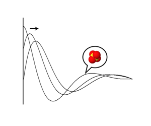
The schematic diagram of the simulation set-up is shown in figure 1. Here, we specify the formulation of wave propagation in rarefied molecular gases confined between two infinite, parallel and impermeable plates located at  $x = 0$ and $x = 1$, which can be treated as a simple prototype of wave propagation in confined space. The plate at $x=0$ may oscillate harmonically at a constant frequency $\omega$ in its normal direction so that the velocity varies as
 \begin{equation} u_w(t) = U_{m}{\rm Re}\{\exp\left({\rm i}{St}\,t\right)\}, \end{equation}
and a sound wave is induced in the gas. This plate may attain unsteady heating so that its temperature varies as
 \begin{equation} T_w(t) = 1+\tau_{m}{\rm Re}\{\exp\left({\rm i}{St}\,t\right)\}, \end{equation}
and a thermal–acoustic wave is consequently induced. In (3.1) and (3.2), ‘ ${\rm i}$’ is the imaginary unit, ${\rm Re}\{{\cdot }\}$ denotes the real part of a complex expression, and $U_m$ and $\tau _m$ are the maximum speed and perturbed temperature of the plate, respectively. The constant ${St}$ is the normalised oscillation frequency, defined as the Strouhal number
 \begin{equation} {St} = \frac{\omega H}{v_{m}}. \end{equation}
Note that the two driving forces have the same frequency. The time-based Knudsen number correlates with  ${Kn}_l$ and ${St}$ through
 \begin{equation} {Kn}_t=\frac{\mu_0\omega}{p_0}=\frac{2{Kn}_l{St}}{\sqrt{\rm \pi}}, \end{equation}
where  $p_0/\mu _0$ is the reference collision frequency of gas molecules.

Figure 1. Schematic diagram of sound and thermal–acoustic wave propagation in rarefied molecular gases between two infinite, parallel and impermeable plates. The oscillating plate is positioned at  $x=0$ with harmonically varying velocity (along the $x$ direction) or temperature, and the stationary plate is at $x=1$. The stationary plate has a fixed temperature of $T_{w}=1$. Both plates are fully diffuse walls.
We are interested in the flow state when the oscillation has been fully established. As a consequence, the time-dependent behaviour of the gas is periodic with the same frequency as the oscillation stimuli. We further assume that the velocity and perturbed temperature of the plate are sufficiently small quantities, i.e.  $u_m\ll 1$ and $\tau _m\ll 1$; hence, the gas system deviates slightly from its reference equilibrium state, which is described by the global Maxwellian
 \begin{equation} E_0 = \frac{I^{d/2-1}}{{\rm \pi} ^{3/2} \varGamma (d/2)} \exp\left(-|\boldsymbol{v}|^2-I\right), \end{equation}
and the kinetic equations can be linearised by representing the distribution function as
 \begin{equation} f(t,x,\boldsymbol{v},I) = E_0[1+{\rm Re}\{h(x,\boldsymbol{v},I)\exp({\rm i}{St}\,t)\}], \end{equation}
where  $|h| \ll 1$ is the amplitude of the perturbed distribution function. The macroscopic flow properties of interest are also expressed by the following complex functions:
 \begin{equation} \left.\begin{gathered}
n(t, x) = 1 + {\rm
Re}\left\{\rho(x)\exp\left({\rm i}{St}\,t\right)\right\},\\
u_x(t,x) = {\rm
Re}\left\{U(x)\exp\left({\rm i}{St}\,t\right)\right\},\\ T_t(t,x)
= 1 + {\rm
Re}\left\{\tau_t(x)\exp\left({\rm i}{St}\,t\right)\right\}, \\
T_r(t,x) = 1 +{\rm
Re}\left\{\tau_r(x)\exp\left({\rm i}{St}\,t\right)\right\},\\
q^x_t(t,x) ={\rm
Re}\left\{Q_t(x)\exp\left({\rm i}{St}\,t\right)\right\},\\
q^x_r(t,x) ={\rm
Re}\left\{Q_r(x)\exp\left({\rm i}{St}\,t\right)\right\},\\
p_{xx}(t,x) =1+{\rm
Re}\left\{P(x)\exp\left({\rm i}{St}\,t\right)\right\},
\end{gathered}\right\}
\end{equation}
\begin{equation} \left.\begin{gathered}
n(t, x) = 1 + {\rm
Re}\left\{\rho(x)\exp\left({\rm i}{St}\,t\right)\right\},\\
u_x(t,x) = {\rm
Re}\left\{U(x)\exp\left({\rm i}{St}\,t\right)\right\},\\ T_t(t,x)
= 1 + {\rm
Re}\left\{\tau_t(x)\exp\left({\rm i}{St}\,t\right)\right\}, \\
T_r(t,x) = 1 +{\rm
Re}\left\{\tau_r(x)\exp\left({\rm i}{St}\,t\right)\right\},\\
q^x_t(t,x) ={\rm
Re}\left\{Q_t(x)\exp\left({\rm i}{St}\,t\right)\right\},\\
q^x_r(t,x) ={\rm
Re}\left\{Q_r(x)\exp\left({\rm i}{St}\,t\right)\right\},\\
p_{xx}(t,x) =1+{\rm
Re}\left\{P(x)\exp\left({\rm i}{St}\,t\right)\right\},
\end{gathered}\right\}
\end{equation}
where  $p_{xx}$ is the gas pressure in the direction of wave propagation. Here $[\rho,U,\tau _t,\tau _t,Q_t,Q_r,P]$ are complex quantities, which can be represented in exponential form as
 \begin{equation} M\left(x\right)=M_{am}\left(x\right)\exp\left[{\rm i}\phi_M\left(x\right)\right],\quad M=\rho,U,\tau_t,\tau_r,Q_t,Q_r,P, \end{equation}
where  $M_{am}$ and $\phi$ are the real functions corresponding to the amplitude and phase of a periodic function. Note that for the spatial coordinates, all the variables depend only on $x$, since the propagation of the wave is restricted to this direction.
Substituting (3.6) and (3.7) into the kinetic equation (2.1) and neglecting all the nonlinear terms, we obtain the equation for  $h$, written as
 \begin{align} {\rm i}St\,h + v_x
\frac{\partial h}{\partial x} &= \delta_0 \left[\rho +
2Uv_x + \tau_t \left(
|\boldsymbol{v}|^{2}-\frac{3}{2}\right)+ \tau_r
\left(I-\frac{d}{2}\right)\right. \nonumber\\ &\quad
+\left.\frac{4}{15}Q_tv_x
\left(|\boldsymbol{v}|^{2}-\frac{5}{2}\right)+
\frac{4}{d}Q_rv_x \left(I-\frac{d}{2}\right)-h\right]
\nonumber\\ &\quad + \frac{\delta}{Z} \left[(\tau -
\tau_t)\left(|\boldsymbol{v}|^2-\frac{3}{2}\right)+(\tau -
\tau_r) \left(I-\frac{d}{2}\right) \right. \nonumber\\
&\left.\quad +\frac{4(Q'-Q_t)
\boldsymbol{v}}{15}\left(|\boldsymbol{v}|^2-\frac{5}{2}\right)+\frac{4(Q''-Q_r)
\boldsymbol{v}}{d} \left(I-\frac{d}{2}\right)\right],
\end{align}
\begin{align} {\rm i}St\,h + v_x
\frac{\partial h}{\partial x} &= \delta_0 \left[\rho +
2Uv_x + \tau_t \left(
|\boldsymbol{v}|^{2}-\frac{3}{2}\right)+ \tau_r
\left(I-\frac{d}{2}\right)\right. \nonumber\\ &\quad
+\left.\frac{4}{15}Q_tv_x
\left(|\boldsymbol{v}|^{2}-\frac{5}{2}\right)+
\frac{4}{d}Q_rv_x \left(I-\frac{d}{2}\right)-h\right]
\nonumber\\ &\quad + \frac{\delta}{Z} \left[(\tau -
\tau_t)\left(|\boldsymbol{v}|^2-\frac{3}{2}\right)+(\tau -
\tau_r) \left(I-\frac{d}{2}\right) \right. \nonumber\\
&\left.\quad +\frac{4(Q'-Q_t)
\boldsymbol{v}}{15}\left(|\boldsymbol{v}|^2-\frac{5}{2}\right)+\frac{4(Q''-Q_r)
\boldsymbol{v}}{d} \left(I-\frac{d}{2}\right)\right],
\end{align}
where  $\tau =(3\tau _t+d\tau _r)/(3+d)$, and $Q'$ and $Q''$ are related to $Q_t$ and $Q_r$ according to (2.6). The boundary condition for $h$ is
 \begin{equation} \left.\begin{gathered}
h^+ = \sqrt{\rm \pi}U_m - 2\sqrt{\rm \pi} \iint _ {v'_x \le 0}
v'_xE_{0}h^{-}\,{\rm d}\boldsymbol{v}'\,{\rm d}I' \\
\quad\quad\quad\quad\quad\quad\qquad\quad +\, 2U_mv_x + \tau_m
\left(|\boldsymbol{v}|^{2}-\frac{5}{2}\right)+
\tau_m\left(I-\frac{d}{2}\right)\quad \text{at}\ x=0,\\
h^+ = 2\sqrt{\rm \pi} \iint _ {v'_x > 0} v'_xE_{0}h^{-}\,{\rm
d}\boldsymbol{v}'\,{\rm d}I'\quad \text{at}\ x=1,
\end{gathered}\right\}
\end{equation}
\begin{equation} \left.\begin{gathered}
h^+ = \sqrt{\rm \pi}U_m - 2\sqrt{\rm \pi} \iint _ {v'_x \le 0}
v'_xE_{0}h^{-}\,{\rm d}\boldsymbol{v}'\,{\rm d}I' \\
\quad\quad\quad\quad\quad\quad\qquad\quad +\, 2U_mv_x + \tau_m
\left(|\boldsymbol{v}|^{2}-\frac{5}{2}\right)+
\tau_m\left(I-\frac{d}{2}\right)\quad \text{at}\ x=0,\\
h^+ = 2\sqrt{\rm \pi} \iint _ {v'_x > 0} v'_xE_{0}h^{-}\,{\rm
d}\boldsymbol{v}'\,{\rm d}I'\quad \text{at}\ x=1,
\end{gathered}\right\}
\end{equation}
where  $h^+$ and $h^-$ denote the reflected and incident perturbed distribution functions. Once $h$ is known, the macro-quantities are calculated from the velocity moments as
 \begin{align} & \left[\rho, U, \tau_t, \tau_r, Q_t, Q_r, P\right] \nonumber\\ &\quad =\iint \left[1, v_x, \frac{2}{3}|\boldsymbol{v}|^{2}-1, \frac{2}{d}I-1, v_x\left(|\boldsymbol{v}|^{2}-\frac{5}{2}\right),v_x \left(I-\frac{d}{2}\right),v^2_x\right]E_{0}h\,{\rm d}\boldsymbol{v}\,{\rm d}I. \end{align}
By introducing complex expressions, the time variable in the governing equation system is eliminated. The technique of computational fluid dynamics for time-independent problems is adopted to find deterministic solutions, which can greatly reduce the computational cost. The details about the computational issues are given in the following section and Appendix A. Note that this method cannot be used to simulate the propagation of a strong wave with large amplitude. In such a circumstance, the assumption that variant flow properties have the same oscillating frequency as the external stimuli may break down, and a weak shock wave may be generated and propagate in space (Cox, Mortell & Reck Reference Cox, Mortell and Reck2001; Tang, Cheng & Xu Reference Tang, Cheng and Xu2001). Then, time-dependent nonlinear kinetic equations should be applied to investigate such flows. Numerical methods with efficient shock-capture schemes, e.g. the unified gas kinetic schemes, should be used (Wang & Xu Reference Wang and Xu2012; Wang et al. Reference Wang, Zhu, Su, Wu and Zhang2018).
4. Results and discussion
In this section, we investigate sound and thermoacoustic wave propagation in rarefied molecular gases. A wide range of rarefactions and oscillation frequencies will be considered. The influence of non-equilibrium relaxations between the translational and rotational modes, in particular the bulk viscosity  $\mu _{b}$ and the Eucken factors $f_{t}$ and $f_{r}$, will be examined.
4.1. Validation of kinetic model and numerical scheme
As the disturbance in the gas is restricted to the  $x$ direction, the dependence of the governing equation system on $v_y$, $v_z$ and $I$ can be eliminated by introducing auxiliary distribution functions that have independent variables $x$ and $v_x$. The details of the reduced system, designed to reduce computational cost, are explained in Appendix A. The kinetic equations are solved by the DVM, where $v_x$ is truncated to the range of $[-6,6]$ and partitioned by $N_v$ non-uniformly distributed points according to
 \begin{equation} v_{x} = \frac{6}{(N_{v}-1)^{3}}({-}N_{v}+1, -N_{v}+3,\ldots, N_{v}-1)^{3}. \end{equation}
In this partition, the majority of the discrete velocities are located around  $v_x=0$; consequently, it is able to capture the discontinuity and rapid oscillation in the perturbed velocity distribution function near $v_x=0$ at the plate positioned at $x=0$ (Kalempa & Sharipov Reference Kalempa and Sharipov2009; Wu Reference Wu2016). We set $N_{v} = 80$, $300$ and $300$ for $Kn = 0.01$, $0.1$ and $10$, respectively, to obtain smooth solutions. The spatial domain $x\in [0,1]$ is divided into $N_{x}$ elements with refinement in the vicinity of the two plates, where the boundary nodes of the elements are calculated by
 \begin{equation} x = s^{3}(10-15s+6s^{2}),\quad s = \frac{(0,1,\ldots,N_{x})}{N_{x}}. \end{equation}
We set  $N_{x} = 64$ for all cases. The spatial derivatives are approximated by the fourth-order discontinuous Galerkin method. To seek stable solutions, a semi-implicit time-iterative scheme is applied and the iteration stops when the residuals of density, velocity and temperature are less than $10^{-7}$. The details of the numerical scheme can be found in Su et al. (Reference Su, Wang, Zhang and Wu2020). The independence of the obtained results on velocity and spatial grids is verified: when the discrete velocities and spatial elements are further doubled, the maximum difference is not larger than $1\,\%$ for the macro-quantities including the pressure amplitude.
We validate our numerical solutions by comparing them with the experimental measurements of Greenspan (Reference Greenspan1959). In the experiment, the working gas was nitrogen, and all measurements were conducted in a two-crystal interferometer. The emitting crystal was fixed and energised at a constant voltage by a crystal-controlled electron-coupled oscillator, generating a sound frequency of approximately 1 MHz. The receiving crystal was connected to a movable slider while the displacement of the crystal receiver was measured. Processed through the filter and amplifier, the change in gas pressure was finally obtained.
The rotational degree of freedom for nitrogen is  $d=2$. For numerical solutions, we set the rotational collision number to $Z = 2.67$ and the thermal relaxation rates to $A_{tt}=0.786$, $A_{tr}=-0.201$, $A_{rt}=-0.059$ and $A_{rr}=0.842$; thus $f_{eu} = 1.993$, $f_{t} = 2.365$ and $f_{r} = 1.435$. These parameters are measured from the DSMC simulation in order to match the total thermal conductivity of nitrogen at $T_0=300$ K obtained from the Rayleigh–Brillouin scattering (Wu et al. Reference Wu, Li, Liu and Ubachs2020; Li et al. Reference Li, Zeng, Su and Wu2021). The numerical and experimental results are compared in terms of the variations of the dimensionless attenuation coefficient $\alpha$ and sound speed $v_{ph}$ against ${Kn}_t$. These acoustic parameters can be expressed in terms of the amplitude $P_{am}$ and $\phi _P$ of the perturbed gas pressure at $x=1$ as
 \begin{equation} \alpha ={-}\sqrt{\frac{\gamma}{2}}\frac{{\mathrm d}\ln P_{am}}{{\mathrm d}{St}},\quad v_{ph} = \frac{c_{0}}{\beta}, \end{equation}
where  $\gamma = 7/5$ is the ratio of specific heats for linear molecules, $c_0$ is the adiabatic sound speed and $\beta$ is the dimensionless phase parameter defined as
 \begin{equation} \beta = \sqrt{\frac{\gamma}{2}}\frac{{\mathrm d}\phi_P}{{\mathrm d}{St}}. \end{equation}
Numerical solutions of  $\alpha$ and $\beta$ are obtained by the pointwise method (Sharipov, Marques Jr & Kremer Reference Sharipov, Marques and Kremer2002; Garcia & Siewert Reference Garcia and Siewert2005; Wang & Xu Reference Wang and Xu2012). The values of $P_{am}$ and $\phi _P$ can be obtained using (3.8a,b).
In the experiment, the Strouhal number  ${St}$ was controlled by adjusting the distance between the sound source and the receptor since the oscillation frequency was fixed. In addition, $P_{am}$ and $\phi _{P}$ depend strongly on ${St}$ (Sharipov et al. Reference Sharipov, Marques and Kremer2002; Struchtrup Reference Struchtrup2012); see figure 2(a,b). When ${St}$ is small, i.e. the source and the receptor are close to each other, distinctive peaks and valleys appear in $P_{am}$ due to resonance. As the distance between the plates grows, no resonance is observed because of the strong damping in a rarefied gas, resulting in a very weak reflected wave. Note that the phase $\phi _P$ also exhibits non-monotonic variations when ${St}$ is small. Since no data were provided for the geometrical set-up of the sound source and receptor in the experiment, in order to eliminate the influence of resonance, $\mathrm {d}(\ln P_{am})/\mathrm {d}St$ and $\mathrm {d}\varPhi _P/\mathrm {d}St$ in (4.3a,b) and (4.4) are determined by the linear tails of the curves in figure 2(a,b). Figure 2(c) shows the comparison between the simulated and measured results, from which we found that our simulations can capture the essential acoustic properties of sound wave propagation in rarefied molecular gases.

Figure 2. Model validation: (a) variation of the pressure amplitude on the receptor with the Strouhal number  ${St}$; (b) variation of the phase on the receptor with ${St}$; (c) comparison of dimensionless sound speed and attenuation coefficient between the simulation results and the experimental data (Greenspan Reference Greenspan1959).
4.2. Investigation of gas damping
Because of energy dissipation, gas damping occurs in sound wave propagation. In this section, the change of pressure amplitude is used to describe the property of gas damping in the flow channel. The gas is nitrogen, and the free parameters  $d$,
$d$,  $Z$ and $A_{ij}$ are the same as those used in the previous section. Figure 3 shows the profile of the pressure amplitude under different ${Kn}_{l}$ and ${St}$.

Figure 3. The change of pressure amplitude in the  $x$ direction: (a) ${St} = 1$; (b) ${St} = 4$; (c) ${St} = 8$. Here ${Kn}_{l}$ is set to 0.01, 0.1, 1 and 10.
In a confined flow, resonance and anti-resonance will appear due to the superposition of incident and reflected waves. The intensity of resonance is determined by the reflected wave as the input energy is constant. In figure 3(a), the collisions between particles are more frequent with smaller  ${St}$ and ${Kn}_{l}$, which means more energy can be transferred to the receptor, resulting in a stronger reflected wave. Consequently, the resonance is stronger as well. It can be seen that the pressure amplitude at the entrance is smaller than that at the receptor because of anti-resonance. With increasing Strouhal number, e.g. ${St} = 4$ in figure 3(b), the reflected wave is weaker and the pressure amplitude at the entrance is larger than that at the receptor when ${Kn}_{l} \geq 0.1$. In figure 3(c), the collisions between particles are infrequent as ${St}$ is large. The resonance becomes obvious when ${Kn}$ is large.
Now we investigate the influence of the bulk viscosity on gas damping. In addition to nitrogen, we consider two more pseudo-gases with the rotational collision number  $Z$ being 113 and 14 250; the other parameters $d$ and $A_{ij}$ remain the same as those for nitrogen. Note that the choice of high $Z$ values was made to investigate the impact of extremely slow relaxation. Previous estimations based on sound attenuation coefficients showed that certain real gases, such as CO $_{2}$, may exhibit large rotational collision numbers and bulk viscosity at low temperature (Cramer Reference Cramer2012). However, recent experimental evidence has indicated that the ratio of the bulk to shear viscosity is approximately 3–5 for CO $_{2}$ at low temperature (Wang, Ubachs & Van De Water Reference Wang, Ubachs and Van De Water2019). Therefore, the high rotational collision number is a result of incorrect splitting of rotational and vibrational modes, and the slow vibrational relaxation should be taken into account when predicting the high attenuation coefficient in CO $_{2}$ (Kustova et al. Reference Kustova, Mekhonoshina, Bechina, Lagutin and Voroshilova2023). For comparison, we also simulate sound wave propagation in a monatomic gas, which is described by the Shakhov equation (Kalempa & Sharipov Reference Kalempa and Sharipov2009). The profiles of pressure amplitude along the flow channel are shown in figure 4. When ${Kn}_{l}$ and/or ${St}$ are relatively large, e.g. ${Kn}_{l} = 0.1$ and ${St} = 8$ or ${Kn}_{l} = 10$ regardless of ${St}$, there is no difference between the simulated gases. This is because the bulk viscosity exerts influence through inelastic collisions; when the degree of rarefaction is high, the molecular collisions are infrequent, so the pressure profiles are not affected by bulk viscosities as they rely on translational energy and there is negligible energy transfer between translational and rotational energies. When ${Kn}_{l}$ and ${St}$ decrease, the particle collisions become more frequent, so the bulk viscosity plays an important role in determining the pressure amplitude. Interestingly, the pressure amplitude of a molecular gas with large bulk viscosity is very close to that of a monatomic gas under all the considered Knudsen and Strouhal numbers. This is because the internal degrees of freedom are frozen when $Z$ is large, i.e. inelastic collisions are rare. The underlying mechanism will be further discussed in § 4.3.

Figure 4. The change of pressure amplitude in the  $x$ direction under various rotational collision numbers. A wide range of rarefaction and oscillation frequencies are simulated: (a) $St = 1$, $Kn_{l} = 0.01$; (b) $St = 1$, $Kn_{l} = 0.1$; (c) $St = 1$, $Kn_{l} = 10$; (d) $St = 8$, $Kn_{l} = 0.01$; (e) $St = 8$, $Kn_{l} = 0.1$; ( f) $St = 8$, $Kn_{l} = 10$.
Now we investigate the influence of thermal conductivity on gas damping by changing the values of the translational and rotational Eucken factors. We keep the rotational collision number  $Z=2.67$, the total Eucken factor $f_{eu} = 1.993$, $A_{tr}=-0.201$ and $A_{rt}=-0.059$ the same as the experimental values for nitrogen. Figure 5 shows the pressure amplitude under translational Eucken factors of $1.5, 2.0$ and $2.5$. The corresponding rotational Eucken factors and the two diagonal elements $A_{tt}$ and $A_{rr}$ can be obtained through (2.12) and (2.13a–c). In contrast to the bulk viscosity, the thermal conductivity exerts limited influence on gas damping over a wide range of ${Kn}_{l}$ and ${St}$.

Figure 5. The change of pressure amplitude in the  $x$ direction under different translational Eucken factors. The gas is nitrogen. A wide range of rarefaction and oscillation frequencies are simulated: (a) $St = 1$, $Kn_{l} = 0.01$; (b) $St = 1$, $Kn_{l} = 0.1$; (c) $St = 1$, $Kn_{l} = 10$; (d) $St = 8$, $Kn_{l} = 0.01$; (e) $St = 8$, $Kn_{l} = 0.1$; ( f) $St = 8$, $Kn_{l} = 10$.
4.3. Surface force on transducer
We now evaluate the surface force on the transducer in molecular gases, which can be obtained from the gas pressure at the plate. Therefore, we focus on the change of gas pressure amplitude at  $x = 0$ under different transport coefficients and flow conditions.
The relationships between the pressure amplitude  $P_{am}$ and the Strouhal number ${St}$ under different rotational collision numbers $Z$ and Knudsen numbers ${Kn}_{l}$ are shown in figure 6. It is found that when ${Kn}_{l}$ is not small, say equal to or larger than 1, the effect of particle collisions can be neglected and the profiles of $P_{am}$ remain nearly unchanged regardless of $Z$. Therefore, we focus on examining the flow properties in three distinct flow regimes: ${Kn}_{l} = 0.01$, ${Kn}_{l} = 0.1$ and ${Kn}_{l} = 10$. In all the flow regimes, as ${St}$ increases, $P_{am}$ decreases until the first anti-resonance frequency and then increases to a peak value, which is referred to as the resonance frequency. After exceeding the first resonance frequency, $P_{am}$ changes slightly and tends to be constant when ${St}$ becomes large. In order to analyse $P_{am}$ quantitatively, we first consider the case where the oscillation frequency is much larger than the mean molecular collision frequency, i.e. when ${Kn}_{l}\, {St} \gg 1$. In this case, the collision term in (3.9) can be neglected (Kalempa & Sharipov Reference Kalempa and Sharipov2009; Wu Reference Wu2016). Therefore, we obtain the reduced equation
 \begin{equation} {\rm i}St \,h + v_{x}\frac{\partial h}{\partial x} = 0. \end{equation}
Combining this with the boundary condition on the left plate, we can finally obtain the value of the pressure amplitude on the transducer ( $x = 0$) at the high-frequency limit as
 \begin{equation} P_{am}(x = 0) \rightarrow \frac{2}{\sqrt{\rm \pi}} + \frac{\sqrt{\rm \pi}}{2} \approx 2. \end{equation}
In figure 6(b,d), when the frequency is large, e.g.  ${St}$ is larger than 6, $P_{am}$ approaches 2. However, when ${Kn}_{l}$ is 0.01 (see figure 6a), $P_{am}$ is slightly less than 2 at large Strouhal numbers owing to the fact that particle collisions are frequent and cannot be neglected.

Figure 6. The relationship between the pressure amplitude and  $St$ under different rotational collision numbers. The results of four flow regimes are shown here: (a) $Kn_{l} = 0.01$, (b) $Kn_{l} = 0.1$, (c) $Kn_{l} = 1$ and (d) $Kn_{l} = 10$. The rotational collision number $Z$ is set to 2.67, 10, 100 and 10 000.
Now, we examine the anti-resonance and resonance frequencies. Through the confined flow channel, the molecules leave the left plate with velocity  $v_{p}$, are reflected by the right plate, and finally return to the left plate. Without collision, the total travel distance for a molecule in the $x$ direction is 2 $H$. Thus, we obtain the following equation:
 \begin{equation} 2H \approx v_{p}\,\delta t, \end{equation}
where  $\delta t$ is the travel time of each molecule. When the travel time satisfies
 \begin{equation} \delta t =
\frac{2n{\rm \pi}}{\omega}\quad {\rm or}\quad
\frac{(2n-1){\rm \pi}}{\omega},\quad n \in N_+,
\end{equation}
\begin{equation} \delta t =
\frac{2n{\rm \pi}}{\omega}\quad {\rm or}\quad
\frac{(2n-1){\rm \pi}}{\omega},\quad n \in N_+,
\end{equation}
the molecules leaving and coming back to the left plate have the same or opposite phase, corresponding to the resonance or anti-resonance point. Replacing  $\omega$ by ${St}$, we finally obtain the resonance frequency $St_{r}$ and anti-resonance frequency $St_a$ as
 $$\begin{gather} St_{r} \approx \frac{v_{p}}{v_{m}} n{\rm \pi},\quad n \in N_+, \end{gather}$$
 $$\begin{gather}St_{a} \approx \frac{v_{p}}{v_{m}} \frac{(2n-1){\rm \pi}}{2}, \quad n \in N_+. \end{gather}$$
For free molecular flow ( $Kn_{l} = 10$), the collisions between particles can be neglected and the travel distance of molecules in the $x$ direction is $2H$. In addition, the gas flow slightly deviates from the global equilibrium state, so $v_{p} \approx v_{m}$. Then, we obtain the first resonance frequency $St_{r} \approx {\rm \pi}\approx 3.14$ and the first anti-resonance frequency $St_{a} \approx {\rm \pi}/2 \approx 1.57$ through (4.9) and (4.10), which are consistent with the results shown in figure 6(d). When ${Kn}_{l} = 0.1$ and ${Kn}_{l} = 0.01$, the increased frequency of collisions makes the free movement of molecules more difficult. Thus, the real travel time of particles is larger than ${2H}/{v_{p}}$. Therefore, the first resonance frequency and anti-resonance frequency are smaller than the respective theoretical values.
The influence of the bulk viscosity on the pressure amplitude at  $x=0$ is also investigated. As shown in figure 6, the bulk viscosity only affects the pressure amplitude in the slip regime ( ${Kn}_{l} = 0.01$). In the transition and free molecular flow regimes ( ${Kn}_{l} = 0.1$ and ${Kn}_{l} = 10$), because of infrequent particle collisions, the bulk viscosity exerts limited influence on $P_{am}$. Therefore, we focus only on the slip flow regime. From figure 6(a), it is found that the value of $P_{am}$ varies at a fixed $St$ for different bulk viscosities. To reveal the underlying physics, we further plot the profile of $P_{am}$ under different rotational collision numbers with different $St$ numbers; see figure 7(a). It can be seen that with increasing $Z$,
$Z$,  $P_{am}$ is first found to monotonically converge to the constant value of a corresponding monatomic gas (i.e. the dotted line in figure 7a). The result indicates that the internal degrees of freedom will be frozen for large bulk viscosities because of negligible inelastic collisions, as we have discussed in § 4.2. We now further explain this phenomenon here. There is only one inelastic collision in a total of $Z$ collisions, which transfers the energy between translational and internal energies. When $Z$ is large, the inelastic collision frequency is low and then internal energy transfer can be ignored within the characteristic time of the flow field, so the pressure amplitude of molecular gases is equal to that of the corresponding monatomic gases. This is called the frozen state or the local thermodynamic equilibrium (Jaeger, Matar & Müller Reference Jaeger, Matar and Müller2018).

Figure 7. (a) The change of pressure amplitude under different rotational collision numbers with  $St = 2.0$, 4.0, 6.0 and 8.0, where the two dotted lines denote argon at $St = 2.0$ and $St = 8.0$; (b) amplitude of the translational, rotational and total temperatures for different rotational collision numbers with $St = 6.0$.
In order to provide more evidence, we plot the change of perturbed temperature under different  $Z$ with ${St} = 6.0$. As shown in figure 7(b), the perturbed rotational temperature $\tau _{r}$ decreases continuously with the increase of $Z$ due to the decrease of inelastic collisions. When the rotational collision number is large, e.g. more than 1000, the perturbed rotational temperature is close to zero. Consequently, the perturbed overall temperature is reduced to $\tau \approx 0.6 \tau _{t}$ for molecular gases ( $d = 2$) as expected theoretically.
Figure 6(a) shows that the bulk viscosity also influences the resonance frequency. Specifically, the emergence of the resonance frequency will be delayed under large bulk viscosities, and this trend is more obvious when  ${St}$ is large. As mentioned previously, when the value of $Z$ is reduced, inelastic collisions become more frequent. Such collisions result in higher rotational energy and lower translational energy of the gas molecules in sound wave propagation. This causes an increase in travel time. Consequently, the resonance frequencies decrease when the bulk viscosity decreases. For instance, when $Z = 2.67$ and 10, the first resonance frequencies are slightly smaller than those of $Z = 100$ and 10 000. In addition, since the resonance state varies with bulk viscosity, the initial variation of $P_{am}$ depends on $St$ as shown in figure 7(a).
The influence of thermal conductivity on the surface force is also investigated. The total Eucken factor is fixed at  $f_{eu} = 1.993$ while the value of $f_{t}$ is varied. As shown in figure 8, the Eucken factor has little influence on the pressure amplitude and the resonance frequency.

Figure 8. The relationship between the pressure amplitude and  $St$ under different translational Eucken factors. Four flow regimes are investigated: (a) $Kn_{l} = 0.01$; (b) $Kn_{l} = 0.1$; (c) $Kn_{l} = 1$; and (d) $Kn_{l} = 10$. The translational Eucken factor $f_{t}$ is set to 1.5, 2 and 2.5.
5. Onsager–Casimir reciprocal relationship
In this section, we examine whether the OCRR also holds for molecular gases. If we consider a weakly non-equilibrium system where some irreversible processes occur, then the corresponding physical law can be described in a general linear form as
 \begin{equation} J_{k} = \sum _{n} \varLambda _{kn}X_{n}, \end{equation}
where  $X_{n}$ are driven forces, $J_{k}$ are conjugated thermodynamic fluxes and $\varLambda _{kn}$ is the matrix of kinetic coefficients. The non-diagonal elements $\varLambda _{kn}$ ( $k\neq n$) contain solutions corresponding to the forces $X_{k}$ and $X_{n}$. If the form of the thermodynamic flow $J_{k}$ is chosen so that the entropy production $s$ in the statistical system is expressed as
 \begin{equation} s = \sum _{k} J_{k}X_{k}, \end{equation}
then the kinetic coefficients satisfy
 \begin{equation} \varLambda_{kn}^{t} = \varLambda_{nk}^{t}, \end{equation}
where the superscript  $t$ means that each coefficient $\varLambda _{kn}$, composed of two solutions $k$ and $n$, is calculated from the time-reverted molecular state of one of these solutions.
From the Boltzmann equation, the thermodynamic fluxes and forces can be identified for gas flows, and the kinetic coefficients are derived as (Sharipov Reference Sharipov2006)
 $$\begin{gather} \varLambda_{kn} =
\int_{\varSigma}\left(\boldsymbol{v} \boldsymbol{\cdot}
\boldsymbol{n} h_{w}^{(k)},h^{(n)}-
\frac{1}{2}h_{w}^{(n)}\right){\rm d} \varSigma - {\rm
i}St\left(\left(h^{(k)}, h^{(n)}\right)\right),
\end{gather}$$
$$\begin{gather} \varLambda_{kn} =
\int_{\varSigma}\left(\boldsymbol{v} \boldsymbol{\cdot}
\boldsymbol{n} h_{w}^{(k)},h^{(n)}-
\frac{1}{2}h_{w}^{(n)}\right){\rm d} \varSigma - {\rm
i}St\left(\left(h^{(k)}, h^{(n)}\right)\right),
\end{gather}$$
 $$\begin{gather}
\varLambda_{kn}^{t} =
\int_{\varSigma}\left(\mathcal{T} \boldsymbol{v}
\boldsymbol{\cdot} \boldsymbol{n}
h_{w}^{(k)},h^{(n)}-\frac{1}{2}h_{w}^{(n)}\right){\rm d}
\varSigma - {\rm i} St\left(\left(\mathcal{T}h^{(k)},
h^{(n)}\right)\right),
\end{gather}$$
$$\begin{gather}
\varLambda_{kn}^{t} =
\int_{\varSigma}\left(\mathcal{T} \boldsymbol{v}
\boldsymbol{\cdot} \boldsymbol{n}
h_{w}^{(k)},h^{(n)}-\frac{1}{2}h_{w}^{(n)}\right){\rm d}
\varSigma - {\rm i} St\left(\left(\mathcal{T}h^{(k)},
h^{(n)}\right)\right),
\end{gather}$$
where  $\varSigma$ represents solid walls that enclose the flow field $\varOmega$, $h_w$ is given by the wall velocity and temperature as
 \begin{equation} h_w=2\boldsymbol{v}\boldsymbol{\cdot}\boldsymbol{u}_w+\tau_w\left(|\boldsymbol{v}|^2-\frac{5}{2}\right)+\tau_w\left(I-\frac{d}{2}\right), \end{equation}
and the binary operations  $({\cdot },{\cdot })$ and $(({\cdot },{\cdot }))$ are defined for the two arbitrary functions as
 $$\begin{gather} \left(\phi, \psi \right) = \iint E_{0}\phi(\boldsymbol{x}, \boldsymbol{v}, I) \psi(\boldsymbol{x}, \boldsymbol{v}, I)\,{\rm d}\boldsymbol{v}\,{\rm d}I, \end{gather}$$
 $$\begin{gather}((\phi, \psi )) = \int_{\varOmega}\left(\phi, \psi \right){\rm d}\boldsymbol{x}. \end{gather}$$
Finally,  $\mathcal {T}$ is the operator reversing the state of molecules in time,
 \begin{equation} \mathcal{T}\phi(\boldsymbol{x}, \boldsymbol{v}, I) = \phi(\boldsymbol{x}, \boldsymbol{v}^{t}, I^{t}), \end{equation}
which is self-conjugate, i.e.
 \begin{equation} \left(\mathcal{T}\phi, \psi\right) = \left(\mathcal{T}\psi, \phi\right). \end{equation}
For the sound wave stimulated by oscillation of the transducer and the thermoacoustic wave induced by a temperature oscillation, the thermodynamic forces are defined as
 \begin{equation} X_{U} = u_{m},\quad X_{T} = \tau_{m}, \end{equation}
and then the perturbed distribution can be expressed as
 \begin{equation} h(x, \boldsymbol{v}, I) = h^{(U)}(x, \boldsymbol{v}, I)X_{U}+h^{(T)}(x, \boldsymbol{v}, I)X_{T}. \end{equation}
In addition,  $h_{w}$ that defines the boundary condition can also be decomposed as
 \begin{equation} h_{w}(x, \boldsymbol{v}, I) = h_{w}^{(U)}(x, \boldsymbol{v}, I)X_{U}+h_{w}^{(T)}(x, \boldsymbol{v}, I)X_{T}, \end{equation}
where
 $$\begin{gather} h_{w}^{(U)} =\left\{\begin{array}{@{}lc} 2v_{x}, & x = 0, \\ 0, & x = 1, \end{array}\right. \end{gather}$$
 $$\begin{gather}h_{w}^{(T)} = \left\{\begin{array}{@{}lc} \left(|\boldsymbol{v}|^{2}-\dfrac{5}{2}\right)+\left(I-\dfrac{d}{2}\right), & x = 0, \\ 0, & x = 1. \end{array}\right. \end{gather}$$
Using the reciprocal relation, i.e. (5.1), the kinetic coefficients given by (5.4) and (5.5), and the self-conjugate property described by (5.10), we obtain
 \begin{align} & \left(\mathcal{T}v_{x}h_{w}^{(U)},h^{(T)}\right)_{x = 0} - \left(\mathcal{T}v_{x}h_{w}^{(U)},h^{(T)}\right)_{x = 1} \nonumber\\ &\quad = \left(\mathcal{T}v_{x}h_{w}^{(T)},h^{(U)}\right)_{x = 0} - \left(\mathcal{T}v_{x}h_{w}^{(T)},h^{(U)}\right)_{x = 1} \nonumber\\ &\qquad +\left(\mathcal{T}v_{x}h_{w}^{(U)},h_{w}^{(T)}\right)_{x = 0} - \left(\mathcal{T}v_{x}h_{w}^{(U)},h_{w}^{(T)}\right)_{x = 1}. \end{align}
Inserting  $h_{w}^{(U)}$ and $h_{w}^{\textrm {T}}$, we have
 \begin{align} \left(\mathcal{T}2|\boldsymbol{v}|^{2}, h^{(T)}\right)_{x = 0} &= \left(\mathcal{T}v_{x}\left(|\boldsymbol{v}|^{2}-\frac{5}{2}\right),h^{(U)}\right)_{x = 0} + \left(\mathcal{T}v_{x}\left(I-\frac{d}{2}\right),h^{(U)}\right)_{x = 0} \nonumber\\ &\quad + \left(\mathcal{T}2|\boldsymbol{v}|^{2}, \left(|\boldsymbol{v}|^{2}-\frac{5}{2}\right)\right)_{x = 0} + \left(\mathcal{T}2|\boldsymbol{v}|^{2}, \left(I-\frac{d}{2}\right)\right)_{x = 0}, \end{align}
and thus
 \begin{equation} P^{(T)} ={-}Q_{t}^{(U)}-Q_{r}^{(U)} ={-}Q^{(U)},\quad x = 0. \end{equation}
 If we use  $h^{(T)}(1-x,\boldsymbol {v},I)$ instead of $h^{(T)}(x,\boldsymbol {v},I)$, the boundary condition is then transformed into
 \begin{equation} h_{w}^{(T)}(1-x) =\left\{\begin{array}{@{}lc} 0, & x = 0,\\ \left(|\boldsymbol{v}|^{2}-\dfrac{5}{2}\right)+\left(I-\dfrac{d}{2}\right), & x = 1. \end{array}\right. \end{equation}
The reciprocal relation gives
 \begin{align} \left(\mathcal{T}2|\boldsymbol{v}|^{2}, h^{(T)}(1-x)\right)_{x = 0} &={-} \left(\mathcal{T}v_{X}\left(|\boldsymbol{v}|^{2}-\frac{5}{2}\right),h^{(U)}(x)\right)_{x = 1} \nonumber\\ &\quad - \left(\mathcal{T}v_{X}\left(I-\frac{d}{2}\right),h^{(U)}(x)\right)_{x = 1}, \end{align}
and thus
 \begin{equation} P^{(T)} = Q_{t}^{(U)}+Q_{r}^{(U)} = Q^{(U)},\quad x = 1. \end{equation}
Therefore, the OCRR for wave propagation in molecular gases is confirmed by (5.18) and (5.21), which show that the magnitude of the deviation of gas pressure at the walls induced by the thermoacoustic wave is equal to the magnitude of the total heat flux (sum of the translational and internal heat fluxes) induced by the sound wave.
We further show the numerical results for the pressure amplitude and the total heat flux under a wide range of  ${St}$ and ${Kn}_{l}$. The results on the transducer and receptor are shown in figure 9. In all the flow regimes, the pressure amplitude in the thermoacoustic wave agrees with the heat flux in the sound wave, suggesting that the OCRR also holds for molecular gases.

Figure 9. The variation of pressure amplitude and heat flux under different  $St$: (a) $x = 0$ and (b) $x = 1$. The solid lines denote the pressure amplitude while the hollow points represent the heat flux. Three colours denote different flow regimes: red represents the slip regime ( $Kn_{l} = 0.01$), blue represents the transition regime ( $Kn_{l} = 0.1$) and yellow represents the free molecular flow regime ( $Kn_{l} = 10$).
The comparison between the pressure amplitude of the thermoacoustic wave and the total heat flux of the sound wave under different values of the bulk viscosity and thermal conductivity is shown in figure 10. The simulation is conducted in the slip regime with  $Kn = 0.01$. It is evident that the OCRR is valid under different values of bulk viscosity and thermal conductivity. From the left column of figure 10, we can see the influence of the bulk viscosity and thermal conductivity on the thermoacoustic wave. In figure 10(a), the resonance frequency is shifted when the bulk viscosity is altered, which is similar to the behaviour of the sound wave. The only difference lies in the value of $P_{am}$. In the case of the thermoacoustic wave, the pressure variation is generated by the oscillation of temperature, resulting in a significantly lower pressure amplitude than that in the sound wave. Figure 10(c,d) shows that thermal conductivity has little influence on the pressure amplitude of the thermoacoustic wave and the heat flux amplitude of the sound wave.

Figure 10. Comparison between the pressure amplitude of the thermoacoustic wave and the total heat flux of the sound wave under different values of the bulk viscosity and thermal conductivity. The pressure amplitude of the thermoacoustic wave is shown in (a,c) while the total heat flux of the sound wave is shown in (b,d).
6. Conclusions
We have investigated sound wave propagation in rarefied molecular gases over a wide range of rarefactions and oscillation frequencies. We first evaluate the influence of the transport coefficients on gas damping, and find that both rarefaction and oscillation frequency affect the pressure amplitude and resonance/anti-resonance of the sound wave. As for the transport coefficients, the bulk viscosity only exerts influence on the pressure amplitude at small  $Kn_{l}$ and $St$. At larger $Kn_{l}$ and $St$, the pressure amplitude is not affected by the bulk viscosity. The pressure amplitude converges to the value of the corresponding monatomic gas as the bulk viscosity increases. Our results show that the internal degrees of freedom are frozen at large bulk viscosity, so the rotational mode has little influence and the results are similar to those for a monatomic gas. Meanwhile, thermal conductivity has a limited effect on the pressure amplitude and the total heat flux of the sound wave.
The propagation of thermoacoustic waves has also been investigated. We have proved, both analytically and numerically, that the OCRR holds for molecular gases.
Acknowledgements
The authors would like to thank L. Gibelli and B. Shan of Edinburgh University, Scotland, and L. Wu of Southern University of Science and Technology, China, for helpful discussions.
Funding
This work is supported by the UK's Engineering and Physical Sciences Research Council under grant number EP/R041938/2. S.L. is also partly funded by the Chinese Scholarship Council.
Declaration of interests
The authors report no conflict of interest.
Appendix A. Derivation of the one-dimensional kinetic model
To reduce the computational cost, we first eliminate the dependency of  $h$ on the rotational energy $I$ by introducing the two reduced distribution functions
 \begin{equation} h_{0} = \int E_{r}^{0}h\,{\rm d}I, \quad h_{1} = \int E_{r}^{0}Ih\,{\rm d}I \end{equation}
and further letting
 \begin{equation} h_{2} = h_{1} - \frac{d}{2}h_{0}, \end{equation}
where the equilibrium distribution function  $E_{r}^{0}$ can be expressed as
 \begin{equation} E_{r}^{0} = \frac{I^{d/2-1}}{\varGamma (d/2)}\exp({-}I). \end{equation}
The governing equations eventually become
 \begin{gather} {\rm i}St \,h_{0} + v_{x}\frac{\partial h_{0}}{\partial x} = \delta\left[\rho+2Uv_{x}+\tau_{t}\left(|\boldsymbol{v}|^{2}-\frac{3}{2}\right)+ \frac{4}{15}Q_{t}v_{x}\left(|\boldsymbol{v}|^{2}-\frac{5}{2}\right)-h_{0}\right] \nonumber\\ \qquad\qquad\qquad\qquad +\, \frac{\delta}{Z}\left[(\tau-\tau_{t})\left(|\boldsymbol{v}|^{2}-\frac{3}{2}\right)+ \frac{4(Q^{\prime}-Q_{t})v_{x}}{15}\left(|\boldsymbol{v}|^{2}-\frac{5}{2}\right)\right], \end{gather}
 \begin{gather} h_{2} + v_{x}\frac{\partial h_{2}}{\partial x} = \delta\left[\frac{d}{2}\tau_{r}-h_{2}\right]+ \frac{d\delta}{2Z}(\tau-\tau_{r}) + \frac{2\delta}{Z}Q^{\prime\prime\prime}v_{x}, \end{gather}
where
 \begin{equation} Q^{\prime\prime\prime} ={-}A_{rt}ZQ_{t}+Z(1-A_{rr})Q_{r}. \end{equation}
The macroscopic quantities are calculated from  $h_{0}$ and $h_{2}$ as
 $$\begin{gather} \left[\rho,U,\tau_{t},Q_{t}\right] = \int \left[1,v_{x},\frac{2}{3}|\boldsymbol{v}|^{2}-1,v_{x} \left(|\boldsymbol{v}|^{2}-\frac{5}{2}\right)\right]E_{t}^{0}h_{0}\,{\rm d} \boldsymbol{v}, \end{gather}$$
 $$\begin{gather}\left[\tau_{r},Q_{r}\right] = \int \left[\frac{2}{d},v_{x}\right]E_{t}^{0}h_{2}\,{\rm d} \boldsymbol{v}. \end{gather}$$
Now we transform the governing equations from the three-dimensional velocity space to the one-dimensional velocity space by introducing the following reduced distributions:
 $$\begin{gather} \varPhi_{0}(x,v_{x}) = \frac{1}{\rm \pi} \int \exp({-}v_{y}^{2}-v_{z}^{2})h_{0}\,{\rm d}v_{y}\,{\rm d}v_{z}, \end{gather}$$
 $$\begin{gather}\varPhi_{1}(x,v_{x}) = \frac{1}{\rm \pi} \int \exp({-}v_{y}^{2}-v_{z}^{2})\left(v_{y}^{2}+v_{z}^{2}-1\right)h_{0}\,{\rm d}v_{y}\,{\rm d}v_{z}, \end{gather}$$
 $$\begin{gather}\varPsi(x,v_{x}) = \frac{1}{\rm \pi} \int \exp({-}v_{y}^{2}-v_{z}^{2})h_{2}\,{\rm d}v_{y}\,{\rm d}v_{z}. \end{gather}$$
Then the governing equations become
 \begin{gather}
{\rm i}St\varPhi_{0} +
v_{x}\frac{\partial \varPhi_{0}}{\partial x} =
\delta\left[\rho+2Uv_{x}+\tau_{t}\left(v_{x}^{2}-\frac{1}{2}\right)+
\frac{4}{15}Q_{t}v_{x}\left(v_{x}^{2}-\frac{3}{2}\right)-\varPhi_{0}\right]
\nonumber\\ \qquad+\,
\frac{\delta}{Z}\left[(\tau-\tau_{t})\left(v_{x}^{2}-\frac{1}{2}\right)+
\frac{4(Q^{\prime}-Q_{t})v_{x}}{15}\left(v_{x}^{2}-\frac{3}{2}\right)\right],
\end{gather}
\begin{gather}
{\rm i}St\varPhi_{0} +
v_{x}\frac{\partial \varPhi_{0}}{\partial x} =
\delta\left[\rho+2Uv_{x}+\tau_{t}\left(v_{x}^{2}-\frac{1}{2}\right)+
\frac{4}{15}Q_{t}v_{x}\left(v_{x}^{2}-\frac{3}{2}\right)-\varPhi_{0}\right]
\nonumber\\ \qquad+\,
\frac{\delta}{Z}\left[(\tau-\tau_{t})\left(v_{x}^{2}-\frac{1}{2}\right)+
\frac{4(Q^{\prime}-Q_{t})v_{x}}{15}\left(v_{x}^{2}-\frac{3}{2}\right)\right],
\end{gather}
 $$\begin{gather} {\rm i}St\varPhi_{1} + v_{x}\frac{\partial \varPhi_{1}}{\partial x} = \delta\left[\tau_{t}+\frac{4}{15}Q_{t}v_{x}-\varPhi_{1}\right] + \frac{\delta}{Z}\left[(\tau-\tau_{t})+\frac{4(Q^{\prime}-Q_{t})v_{x}}{15}\right], \end{gather}$$
 $$\begin{gather}\varPsi + v_{x}\frac{\partial \varPsi}{\partial x} = \delta\left[\frac{d}{2}\tau_{r}-\varPsi\right]+\frac{d\delta}{2Z}(\tau-\tau_{r}) + \frac{2\delta}{Z}Q^{\prime\prime\prime}v_{x}. \end{gather}$$
The full diffuse boundary conditions for  $\varPhi _{0}$, $\varPhi _{1}$ and $\varPsi$ can be obtained using
 $$\begin{gather} \varPhi_{0}(x = 0,v_{x} > 0) = \sqrt{\rm \pi}U_{m}-2\sqrt{\rm \pi}\int_{v_{x} \le 0} v_{x}E_{t}^{01}\varPhi_{0}\,{\boldsymbol d}v_{x} + 2U_{m}v_{x}+\tau_{m}(v_{x}^{2}-1), \end{gather}$$
 $$\begin{gather}\varPhi_{0}(x = 1,v_{x} < 0) = \sqrt{\rm \pi}U_{m}+2\sqrt{\rm \pi}\int_{v_{x} \geq 0} v_{x}E_{t}^{01}\varPhi_{0}\,{\boldsymbol d}v_{x} + 2U_{m}v_{x}+\tau_{m}(v_{x}^{2}-1), \end{gather}$$
 $$\begin{gather}\varPhi_{1}(x = 1,v_{x} < 0) = \varPhi_{1}(x = 1,v_{x} > 0) = \tau_{w}\left(v_{x}^{2}-\frac{3}{2}\right), \end{gather}$$
 $$\begin{gather}\varPsi(x = 1,v_{x} < 0) = \varPsi(x = 1,v_{x} > 0) = \frac{d}{2}\tau_{w}, \end{gather}$$
with the equilibrium distribution function
 \begin{equation} E_{t}^{01} = \frac{1}{\sqrt{\rm \pi}}\exp({-}v_{x}^{2}). \end{equation}
The macroscopic quantities can be calculated using
 \begin{gather} \left[\rho,U,\tau_{t},Q_{t}\right] = \int \left[1,v_{x},\frac{2}{3}\left(v_{x}^{2}-\frac{1}{2}\right),v_{x} \left(v_{x}^{2}-\frac{3}{2}\right)\right]E_{t}^{01}\varPhi_{0}\,{\rm d} v_{x} \nonumber\\ \qquad +\,\int \left[0,0,\frac{2}{3},v_{x}\right]E_{t}^{01}\varPhi_{1}\,{\rm d} v_{x}, \end{gather}
 \begin{gather} \left[\tau_{r},Q_{r}\right] = \int \left[\frac{2}{d},v_{x}\right]E_{t}^{01}\varPsi\,{\rm d}v_{x}. \end{gather}


