1 Introduction
The series of experiments described in Kowal & Worster (Reference Kowal and Worster2015) involving two superposed currents of viscous fluids of different viscosity flowing radially outwards revealed a novel cross-flow fingering instability when the lower layer is less viscous. A sample sequence of photographs of the fingering instability is shown in figure 1. The instability occurs at late stages of the experiments, causing lobes of highly lubricated, thin regions of high-viscosity fluid to advance ahead of less mobile, thicker regions of high-viscosity fluid. Despite its characteristically different formation mechanism, there are similarities between the instability observed in the experiments of Kowal & Worster (Reference Kowal and Worster2015) and the well-known Saffman–Taylor instability, involving the intrusion of a less viscous fluid into a more viscous fluid in a porous medium (Saffman & Taylor Reference Saffman and Taylor1958) or Hele-Shaw cell. Viscous fingering is ubiquitous in nature and industry and may result in complex, highly branched structures (Saffman & Taylor Reference Saffman and Taylor1958; Paterson Reference Paterson1981; Homsy Reference Homsy1987; Chen Reference Chen1989; Thome et al. Reference Thome, Rabaud, Hakim and Couder1989; Manickam & Homsy Reference Manickam and Homsy1993). Similar phenomena are prevalent in various scenarios, such as in oil recovery processes (Orr & Taber Reference Orr and Taber1984), carbon sequestration (Cinar, Riaz & Tchelepi Reference Cinar, Riaz and Tchelepi2009), coating applications and ribbing (Taylor Reference Taylor1963; Reinelt Reference Reinelt1995) and morphological instabilities in crystal growth (Mullins & Sekerka Reference Mullins and Sekerka1964). The patterns that emerge may be controlled by varying the injection rate of the less viscous fluid (Li et al. Reference Li, Lowengrub, Fontana and Palffy-Muhoray2009; Dias & Miranda Reference Dias and Miranda2010; Dias et al. Reference Dias, Alvarez-Lacalle, Carvalho and Miranda2012), changing the geometry (Nase, Derks & Lindner Reference Nase, Derks and Lindner2011; Al-Housseiny, Tsai & Stone Reference Al-Housseiny, Tsai and Stone2012; Juel Reference Juel2012; Dias & Miranda Reference Dias and Miranda2013) and elasticity (Pihler-Puzovic et al. Reference Pihler-Puzovic, Illien, Heil and Juel2012, Reference Pihler-Puzovic, Perillat, Russell, Juel and Heil2013; Pihler-Puzovic, Juel & Heil Reference Pihler-Puzovic, Juel and Heil2014) of the medium, by the use of anisotropy (Ben-Jacob et al. Reference Ben-Jacob, Godbey, Goldenfeld, Koplik, Levine, Mueller and Sander1985), and the use of non-Newtonian fluids (Kondic, Shelley & Palffy-Muhoray Reference Kondic, Shelley and Palffy-Muhoray1998; Fast et al. Reference Fast, Kondic, Shelley and Palffy-Muhoray2001; Kagei, Kanie & Kawaguchi Reference Kagei, Kanie and Kawaguchi2005).
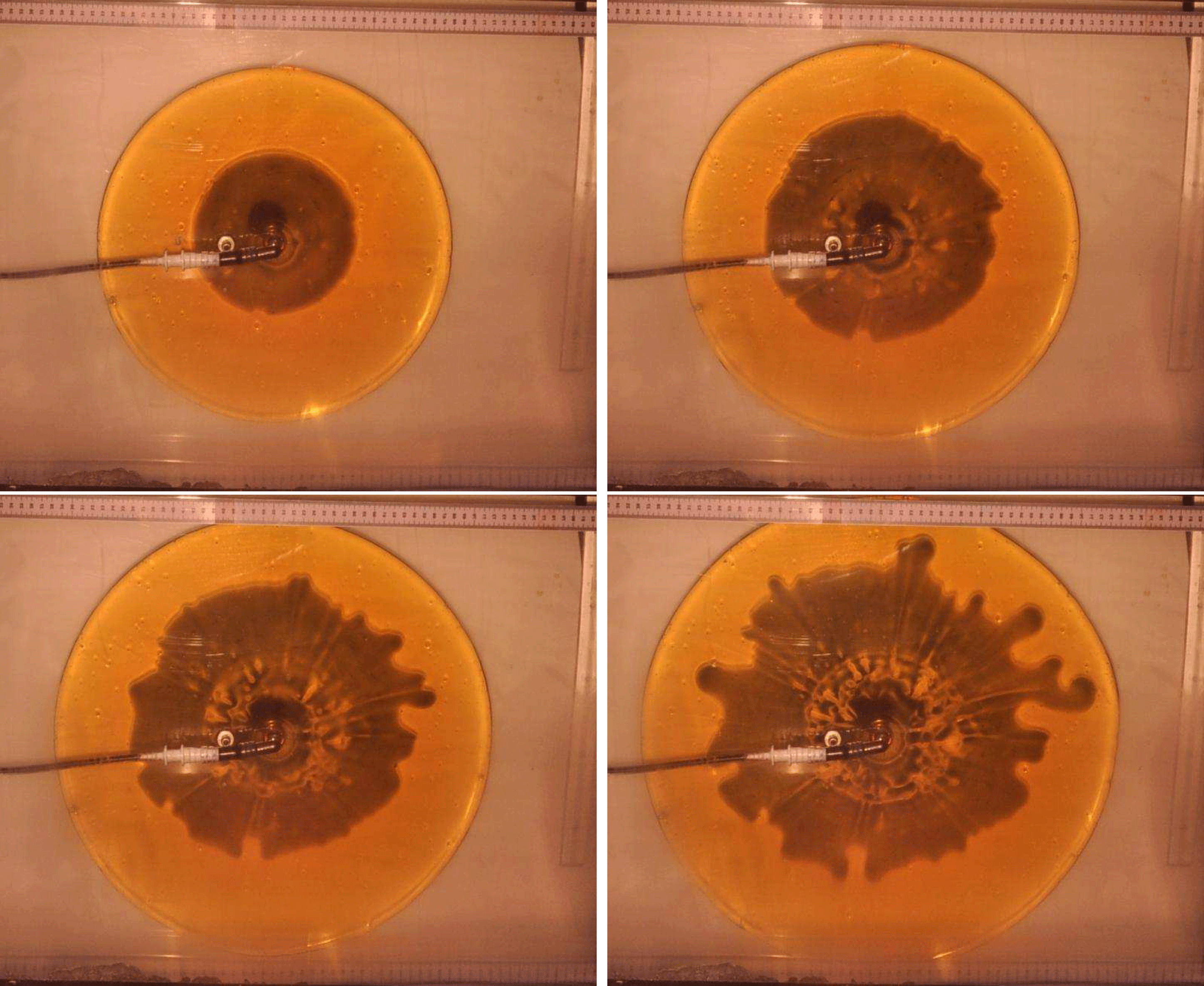
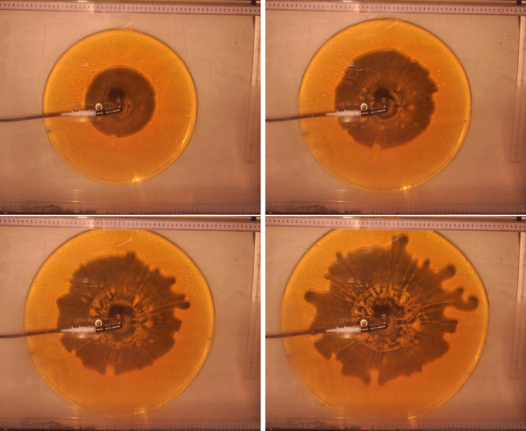
Figure 1. Photographs of the bottom view of one of our experiments
 $t=100$
, 200, 300 and 400 seconds after injection of the lubricant. Less viscous fluid (dyed potassium carbonate solution) intrudes underneath a more viscous fluid (golden syrup).
$t=100$
, 200, 300 and 400 seconds after injection of the lubricant. Less viscous fluid (dyed potassium carbonate solution) intrudes underneath a more viscous fluid (golden syrup).
These frontal instabilities can be contrasted with the internal instabilities that arise between co-flowing, superposed viscous fluids. It has been found by Yih (Reference Yih1967), for example, that a contrast in the viscosities of two superposed fluid films between two horizontal plates can cause long-wavelength instabilities and lead to the formation of wavy patterns. This became commonly known for affecting the quality of manufactured products in industrial processes and attracted a breadth of research on the subject, focusing on flows in two spatial dimensions (Kao Reference Kao1968; Wang, Seaborg & Lin Reference Wang, Seaborg and Lin1978; Hooper & Boyd Reference Hooper and Boyd1983, Reference Hooper and Boyd1987; Hinch Reference Hinch1984; Hooper & Grimshaw Reference Hooper and Grimshaw1985; Renardy Reference Renardy1987; Hooper Reference Hooper1989; Chen Reference Chen1993; Tilley, Davis & Bankoff Reference Tilley, Davis and Bankoff1994; Balmforth, Craster & Toniolo Reference Balmforth, Craster and Toniolo2003). Loewenherz & Lawrence (Reference Loewenherz and Lawrence1989) and Loewenherz, Lawrence & Weaver (Reference Loewenherz, Lawrence and Weaver1989) later related these results in a glaciological context to the formation of transverse ridges on rock glaciers. The above-mentioned studies of instabilities due to a viscosity difference between two superposed fluid films are all concerned with an internal instability mechanism and do not involve the cross-flow dimension. The resulting instabilities are longitudinal, in contrast to the fingering patterns observed in the experiments of Kowal & Worster (Reference Kowal and Worster2015).
The experiments of Kowal & Worster (Reference Kowal and Worster2015) were motivated by considerations of subglacial till, or water-saturated subglacial sediment, which lubricates the underside of glacial ice sheets, such as those of Greenland and Antarctica, in an idealised experimental setting that aids flow delivery. The parts of the experiments relevant to the glaciological setting are their internal dynamics, particularly the viscous coupling between the two layers, rather than their frontal dynamics, at the intrusion front, and it is of interest to determine which of these give rise to the instabilities. In particular, can the instabilities give insight into the formation of ice streams, or regions of ice that are much faster flowing than their surroundings? Their formation has been suggested to result from a spontaneous instability of ice flow through a positive feedback between sliding velocity and basal-melt production (Fowler & Johnson Reference Fowler and Johnson1995, Reference Fowler and Johnson1996; Sayag & Tziperman Reference Sayag and Tziperman2008), a triple-valued sliding law (Sayag & Tziperman Reference Sayag and Tziperman2009; Kyrke-Smith, Katz & Fowler Reference Kyrke-Smith, Katz and Fowler2014) or thermoviscous fingering (Payne & Dongelmans Reference Payne and Dongelmans1997; Hindmarsh Reference Hindmarsh2004, Reference Hindmarsh2006). The last of these has also been seen in the context of the surface cooling of viscoplastic lava domes (Balmforth & Craster Reference Balmforth and Craster2000).
In this paper, we analyse the origins of the instability by posing questions as to what the possible instability mechanisms might be and formulating simpler problems that specifically isolate each mechanism. Two main questions arise: is the instability an internal instability, arising from internal dynamics, or is it a frontal instability, arising from viscous intrusion?
To answer the first question, we consider a problem in which both fluids drain off the edge of a finite plate, as shown in figure 2(a). This setting allows us to focus on internal dynamics while frontal dynamics play no role. The nature of the problem allows for a clean proof that all normal-mode disturbances for any parameter values have negative growth rates. This proves stability for all parameter values and suggests that the experimentally observed instabilities are frontal instabilities. We present the proof in § 3 after introducing the governing equations in § 2. The mechanism of instability is revealed first in § 4 (specifically in § 4.1) by considering frontal dynamics, and then modified in §§ 5 and 6.
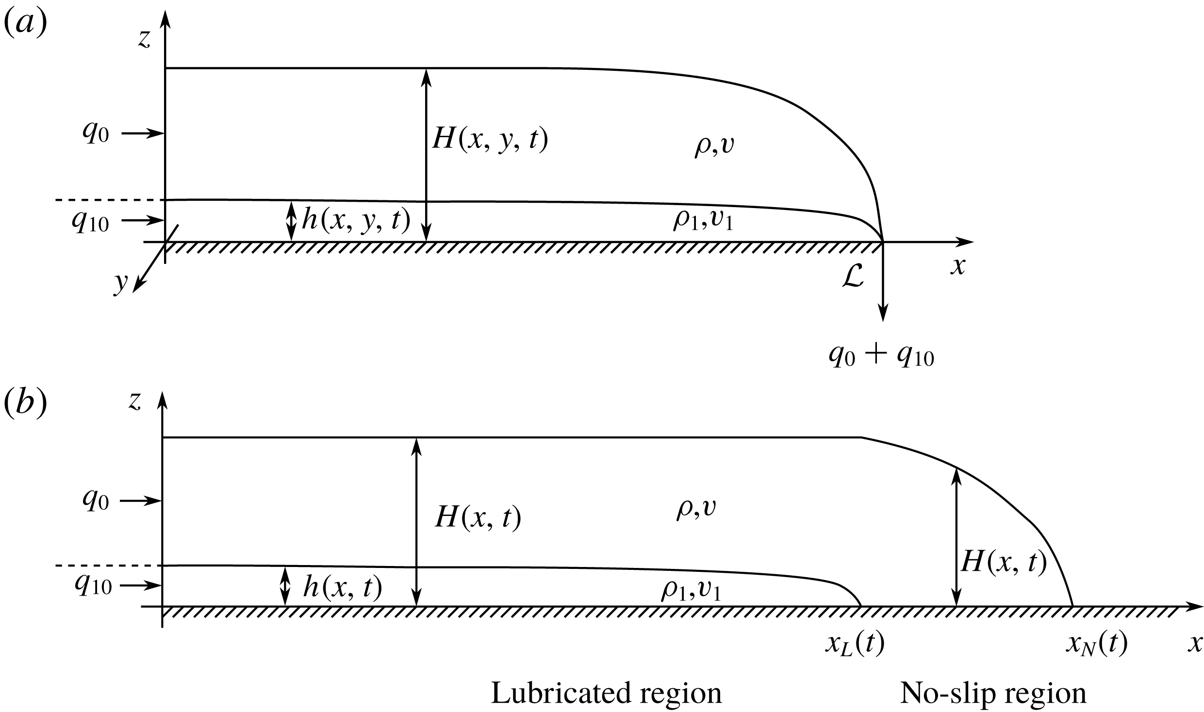
Figure 2. Schematic of two superposed thin films of viscous fluid spreading horizontally under gravity on a rigid horizontal surface with (a) and without (b) drainage at
 $x={\mathcal{L}}$
off the edge of the rigid plate. (a) Thin films of fluid spreading over a finite plate in steady state. (b) A spreading current with an internal lubrication front. Panel (b) is reproduced from Kowal & Worster (Reference Kowal and Worster2015).
$x={\mathcal{L}}$
off the edge of the rigid plate. (a) Thin films of fluid spreading over a finite plate in steady state. (b) A spreading current with an internal lubrication front. Panel (b) is reproduced from Kowal & Worster (Reference Kowal and Worster2015).
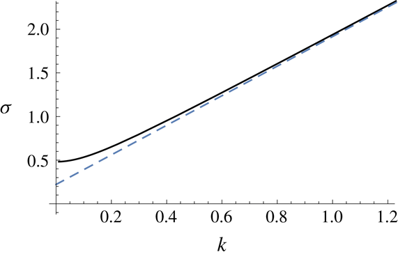
To examine frontal dynamics, we focus the remaining sections of this paper on a stability analysis in the neighbourhood of the lubrication front, where the instability originates. In § 4, we focus on a singular limit in which the densities of the two layers are equal. As a consequence, the order of the governing equations reduces by one and the frontal singularity, which occurs at the tip of the intruding current only when there is a density difference between the layers, reduces to a frontal jump discontinuity (Kowal & Worster Reference Kowal and Worster2015). This allows for a local linear approximation to the surface slopes of both layers in the inner region near the lubrication front. In this set-up, we characterise conditions under which the flow is unstable and identify the underlying instability mechanism. We find that although the physics of this problem reveals the mechanism of instability, it does not yield a stabilising mechanism for wavelength selection.
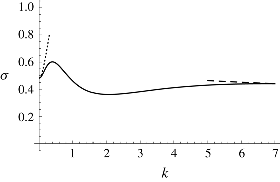
We devote the remaining part of this paper to explore the effect of transverse shear as a possible large-wavenumber stabilising mechanism in two dynamical regimes and develop a thin-film theory in each of these. The first regime, described in § 5, is one in which the wavelength of the perturbations is much smaller than the thickness of both layers of fluid, in which case the flow of the perturbations is resisted dominantly by horizontal shear stresses. These stabilise small wavelengths. The physical ideas of §§ 4 and 5 are combined in § 6 to determine wavelength selection at intermediate wavenumbers. This final regime is an intermediate regime accounting for both vertical and horizontal shear stresses. We note that this is an idealised scenario, in which only vertical and horizontal shear stresses appear, and the purpose is to determine whether or not these are sufficient to provide stabilisation at large wavenumbers. However, we also note that extensional stress gradients may also become important at similar length scales, prompting the need for a solution to the full Stokes equations near the intrusion front, which we do not attempt in this paper.
We perform a more detailed analysis of the full problem, in which the densities of the two layers are not assumed equal and without the use of local spatial and frozen-time approximations, in the companion paper (Kowal & Worster Reference Kowal and Worster2019). The companion paper can be read alone, without absorbing all the details of the current paper.
2 Governing equations for lubricated currents
In the present paper, we adopt a two-dimensional geometry for the basic states that we consider. The experiments of Kowal & Worster (Reference Kowal and Worster2015) were carried out in an initially axisymmetric geometry and the companion paper analyses the stability for an axisymmetric basic state. We find in the companion paper that the mechanism of instability and the conditions of the onset of instability are unaffected by the change in geometry.
The following is based on the PhD thesis by Kowal (Reference Kowal2016). The systems we analyse are illustrated in figure 2. The lubricated region in each case consists of two superposed layers of fluid spreading horizontally under their own weight over a rigid plate. We denote the height of the interface between the two fluids by
 $h(x,y,t)$
and the upper surface height by
$h(x,y,t)$
and the upper surface height by
 $H(x,y,t)$
. The fluids are of different dynamic viscosities
$H(x,y,t)$
. The fluids are of different dynamic viscosities
 $\unicode[STIX]{x1D707}$
and
$\unicode[STIX]{x1D707}$
and
 $\unicode[STIX]{x1D707}_{l}$
, kinematic viscosities
$\unicode[STIX]{x1D707}_{l}$
, kinematic viscosities
 $\unicode[STIX]{x1D708}$
and
$\unicode[STIX]{x1D708}$
and
 $\unicode[STIX]{x1D708}_{l}$
, densities
$\unicode[STIX]{x1D708}_{l}$
, densities
 $\unicode[STIX]{x1D70C}$
and
$\unicode[STIX]{x1D70C}$
and
 $\unicode[STIX]{x1D70C}_{l}~({\geqslant}\unicode[STIX]{x1D70C})$
, and are released at fixed source fluxes
$\unicode[STIX]{x1D70C}_{l}~({\geqslant}\unicode[STIX]{x1D70C})$
, and are released at fixed source fluxes
 $q_{0}$
and
$q_{0}$
and
 $q_{l0}$
, where the subscript
$q_{l0}$
, where the subscript
 $l$
refers to the lower layer. The gravitational constant is denoted by
$l$
refers to the lower layer. The gravitational constant is denoted by
 $g$
. Three important dimensionless parameters arise, namely the dynamic viscosity ratio, the dimensionless density difference and the flux ratio between the two fluids, given by
$g$
. Three important dimensionless parameters arise, namely the dynamic viscosity ratio, the dimensionless density difference and the flux ratio between the two fluids, given by
 $$\begin{eqnarray}{\mathcal{M}}=\frac{\unicode[STIX]{x1D707}}{\unicode[STIX]{x1D707}_{l}},\quad {\mathcal{D}}=\frac{\unicode[STIX]{x1D70C}_{l}-\unicode[STIX]{x1D70C}}{\unicode[STIX]{x1D70C}}\quad \text{and}\quad {\mathcal{Q}}=\frac{q_{l0}}{q_{0}},\end{eqnarray}$$
respectively. Although the following applies for viscous fluids with general viscosity ratios, we are principally interested in the case in which the lower layer is less viscous, lubricating the overlying highly viscous current.
The dynamics of the underlying current is dominated by vertical shear stresses arising from traction along the rigid plate. However, shear and extensional stresses can both play a role within the overlying current. As in Kowal & Worster (Reference Kowal and Worster2015), we consider the limit in which vertical shear provides the dominant resistance to the flow in both layers. We assume that inertia and the effects of mixing and surface tension at the interface between the layers are negligible and consider a balance between viscous and buoyancy forces. We assume that the films are much thinner than their extent,
 ${\mathcal{H}}\ll {\mathcal{L}}$
, where
${\mathcal{H}}\ll {\mathcal{L}}$
, where
 ${\mathcal{H}}$
and
${\mathcal{H}}$
and
 ${\mathcal{L}}$
are the characteristic thickness and length of the flow, and apply the approximations of lubrication theory.
${\mathcal{L}}$
are the characteristic thickness and length of the flow, and apply the approximations of lubrication theory.
We apply the following non-dimensionalisation throughout:
 $$\begin{eqnarray}x={\mathcal{L}}\tilde{x},\quad (H,h)={\mathcal{H}}(\tilde{H},\tilde{h}),\quad t={\mathcal{T}}\,\tilde{t},\quad (\boldsymbol{q},\boldsymbol{q}_{\boldsymbol{l}})=q_{0}(\tilde{\boldsymbol{q}},\tilde{\boldsymbol{q}_{l}}),\end{eqnarray}$$
where
 $$\begin{eqnarray}{\mathcal{H}}=\left(\frac{\unicode[STIX]{x1D708}q_{0}{\mathcal{L}}}{g}\right)^{1/4}\quad \text{and}\quad {\mathcal{T}}=\left(\frac{\unicode[STIX]{x1D708}{\mathcal{L}}^{5}}{gq_{0}^{3}}\right)^{1/4}\end{eqnarray}$$
are the characteristic thickness and time scales of the currents associated with a length scale
 ${\mathcal{L}}$
, which depends on the problem in question and will be specified in the appropriate sections. We drop tildes henceforth.
${\mathcal{L}}$
, which depends on the problem in question and will be specified in the appropriate sections. We drop tildes henceforth.
The horizontal fluid velocities satisfy
 $$\begin{eqnarray}\unicode[STIX]{x1D707}\boldsymbol{u}_{zz}=\unicode[STIX]{x1D735}p\quad \text{for }h\leqslant z\leqslant H,\quad \unicode[STIX]{x1D707}_{l}\boldsymbol{u}_{lzz}=\unicode[STIX]{x1D735}p_{l}\quad \text{for }0\leqslant z\leqslant h,\end{eqnarray}$$
where
 $\unicode[STIX]{x1D735}$
is the horizontal component of the gradient operator, and the pressures are given by
$\unicode[STIX]{x1D735}$
is the horizontal component of the gradient operator, and the pressures are given by
 $$\begin{eqnarray}\displaystyle & p=(H-z)\quad \text{for }h\leqslant z\leqslant H, & \displaystyle\end{eqnarray}$$
 $$\begin{eqnarray}\displaystyle & \displaystyle p_{l}=(H-h)+\frac{\unicode[STIX]{x1D70C}_{l}}{\unicode[STIX]{x1D70C}}(h-z)\quad \text{for }0\leqslant z\leqslant h. & \displaystyle\end{eqnarray}$$
These are subject to no slip at the base, no stress at the upper, free surface,
 $$\begin{eqnarray}\boldsymbol{u}_{\boldsymbol{l}}=0\quad (z=0),\quad \unicode[STIX]{x1D707}\boldsymbol{u}_{z}=0\quad (z=H),\end{eqnarray}$$
and continuity of velocity and shear stress between the layers,
 $$\begin{eqnarray}\boldsymbol{u}_{\boldsymbol{l}}=\boldsymbol{u},\quad \unicode[STIX]{x1D707}_{l}\boldsymbol{u}_{lz}=\unicode[STIX]{x1D707}\boldsymbol{u}_{z}\quad (z=h).\end{eqnarray}$$
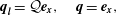
These equations can be solved and integrated to obtain the volume flux of fluid, per unit width, in the lower and upper films:
 $$\begin{eqnarray}\boldsymbol{q}_{\boldsymbol{l}}=\int _{0}^{h}\boldsymbol{u}_{\boldsymbol{ l}}\,\text{d}z=-\left[\frac{{\mathcal{M}}}{3}h^{3}({\mathcal{D}}\unicode[STIX]{x1D735}h+\unicode[STIX]{x1D735}H)+\frac{1}{2}{\mathcal{M}}h^{2}(H-h)\unicode[STIX]{x1D735}H\right],\end{eqnarray}$$
 $$\begin{eqnarray}\displaystyle \boldsymbol{q} & = & \displaystyle \int _{h}^{H}\boldsymbol{u}\,\text{d}z=-\left[\frac{1}{3}(H-h)^{3}\unicode[STIX]{x1D735}H\right.\nonumber\\ \displaystyle & & \displaystyle +\left.\frac{1}{2}{\mathcal{M}}h^{2}(H-h)({\mathcal{D}}\unicode[STIX]{x1D735}h+\unicode[STIX]{x1D735}H)+{\mathcal{M}}h(H-h)^{2}\unicode[STIX]{x1D735}H\right].\end{eqnarray}$$
In each film, there are Poiseuille-like contributions from the spreading of each film under its own weight and Couette-like contributions arising from boundary motion (Kowal & Worster Reference Kowal and Worster2015). These are supplemented by mass conservation equations for the two layers
 $$\begin{eqnarray}\frac{\unicode[STIX]{x2202}h}{\unicode[STIX]{x2202}t}=-\unicode[STIX]{x1D735}\boldsymbol{\cdot }\boldsymbol{q}_{\boldsymbol{l}},\quad \frac{\unicode[STIX]{x2202}(H-h)}{\unicode[STIX]{x2202}t}=-\unicode[STIX]{x1D735}\boldsymbol{\cdot }\boldsymbol{q}\end{eqnarray}$$
and source flux boundary conditions
 $$\begin{eqnarray}\boldsymbol{q}_{\boldsymbol{l}}={\mathcal{Q}}\boldsymbol{e}_{\boldsymbol{x}},\quad \boldsymbol{q}=\boldsymbol{e}_{\boldsymbol{x}}\quad (x=0).\end{eqnarray}$$
The remaining boundary conditions depend on the problem in question and will be discussed as they arise.
3 Internal dynamics: lubricated currents with drainage
Consider two superposed layers of fluid spreading horizontally and steadily under their own weight over a rigid plate of finite length
 $L$
as depicted in figure 2(a). For the non-dimensionalisation (2.2), we take
$L$
as depicted in figure 2(a). For the non-dimensionalisation (2.2), we take
 ${\mathcal{L}}=L$
in this section. Both fluids are pinned at the singular drainage front, that is,
${\mathcal{L}}=L$
in this section. Both fluids are pinned at the singular drainage front, that is,
 $$\begin{eqnarray}h=0,\quad H=0\quad (x=1).\end{eqnarray}$$
3.1 Steady solution
The mass conservation equations admit steady solutions that satisfy
 $$\begin{eqnarray}\boldsymbol{q}_{\boldsymbol{l}}={\mathcal{Q}}\boldsymbol{e}_{\boldsymbol{x}},\quad \boldsymbol{q}=\boldsymbol{e}_{\boldsymbol{x}},\end{eqnarray}$$
along with (3.1). These equations can be solved analytically to yield the two-dimensional steady solutions
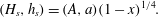 $$\begin{eqnarray}(H_{s},h_{s})=(A,a)(1-x)^{1/4}.\end{eqnarray}$$
The constants
 $A$
and
$A$
and
 $a$
depend on the dimensionless parameters through the algebraic conditions given in (A 1) and (A 2) in appendix A.
$a$
depend on the dimensionless parameters through the algebraic conditions given in (A 1) and (A 2) in appendix A.
3.2 Linear perturbation equations
We investigate the linear stability of the steady basic state of § 3.1 by introducing small disturbances
 $h_{p}$
,
$h_{p}$
,
 $H_{p}\ll 1$
. These give rise to the following linearised perturbation fluxes:
$H_{p}\ll 1$
. These give rise to the following linearised perturbation fluxes:
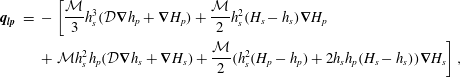 $$\begin{eqnarray}\displaystyle \boldsymbol{q}_{\boldsymbol{l}\boldsymbol{p}} & = & \displaystyle -\left[\frac{{\mathcal{M}}}{3}h_{s}^{3}({\mathcal{D}}\unicode[STIX]{x1D735}h_{p}+\unicode[STIX]{x1D735}H_{p})+\frac{{\mathcal{M}}}{2}h_{s}^{2}(H_{s}-h_{s})\unicode[STIX]{x1D735}H_{p}\right.\nonumber\\ \displaystyle & & \displaystyle +\left.{\mathcal{M}}h_{s}^{2}h_{p}({\mathcal{D}}\unicode[STIX]{x1D735}h_{s}+\unicode[STIX]{x1D735}H_{s})+\frac{{\mathcal{M}}}{2}(h_{s}^{2}(H_{p}-h_{p})+2h_{s}h_{p}(H_{s}-h_{s}))\unicode[STIX]{x1D735}H_{s}\right],\end{eqnarray}$$
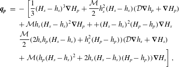 $$\begin{eqnarray}\displaystyle \boldsymbol{q}_{\boldsymbol{p}} & = & \displaystyle -\left[\frac{1}{3}(H_{s}-h_{s})^{3}\unicode[STIX]{x1D735}H_{p}+\frac{{\mathcal{M}}}{2}h_{s}^{2}(H_{s}-h_{s})({\mathcal{D}}\unicode[STIX]{x1D735}h_{p}+\unicode[STIX]{x1D735}H_{p})\right.\nonumber\\ \displaystyle & & \displaystyle +\,{\mathcal{M}}h_{s}(H_{s}-h_{s})^{2}\unicode[STIX]{x1D735}H_{p}++(H_{s}-h_{s})^{2}(H_{p}-h_{p})\unicode[STIX]{x1D735}H_{s}\nonumber\\ \displaystyle & & \displaystyle \frac{{\mathcal{M}}}{2}(2h_{s}h_{p}(H_{s}-h_{s})+h_{s}^{2}(H_{p}-h_{p}))({\mathcal{D}}\unicode[STIX]{x1D735}h_{s}+\unicode[STIX]{x1D735}H_{s})\nonumber\\ \displaystyle & & \displaystyle +\left.{\mathcal{M}}(h_{p}(H_{s}-h_{s})^{2}+2h_{s}(H_{s}-h_{s})(H_{p}-h_{p}))\unicode[STIX]{x1D735}H_{s}\vphantom{\frac{{\mathcal{M}}}{2}}\right],\end{eqnarray}$$
and mass conservation equations
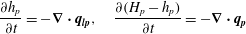 $$\begin{eqnarray}\frac{\unicode[STIX]{x2202}h_{p}}{\unicode[STIX]{x2202}t}=-\unicode[STIX]{x1D735}\boldsymbol{\cdot }\boldsymbol{q}_{\boldsymbol{l}\boldsymbol{p}},\quad \frac{\unicode[STIX]{x2202}(H_{p}-h_{p})}{\unicode[STIX]{x2202}t}=-\unicode[STIX]{x1D735}\boldsymbol{\cdot }\boldsymbol{q}_{\boldsymbol{p}}\end{eqnarray}$$
for the perturbed lower and upper layers, respectively. We impose the boundary conditions
 $$\begin{eqnarray}\boldsymbol{q}_{\boldsymbol{l}\boldsymbol{p}}\boldsymbol{\cdot }\boldsymbol{e}_{\boldsymbol{x}}=0,\quad \boldsymbol{q}_{\boldsymbol{p}}\boldsymbol{\cdot }\boldsymbol{e}_{\boldsymbol{x}}=0\quad (x=0),\end{eqnarray}$$
 $$\begin{eqnarray}h_{p}=0,\quad H_{p}=0\quad (x=1).\end{eqnarray}$$
That is, it is required that the source fluxes of both fluids remain fixed and that both fluids drain at the nose.
We search for normal-mode solutions proportional to
 $\text{e}^{\unicode[STIX]{x1D70E}t+\text{i}ky}$
with amplitudes
$\text{e}^{\unicode[STIX]{x1D70E}t+\text{i}ky}$
with amplitudes
 $\tilde{h}_{p}(x)$
,
$\tilde{h}_{p}(x)$
,
 $\tilde{H}_{p}(x)$
. Here,
$\tilde{H}_{p}(x)$
. Here,
 $k$
is the transverse wavenumber of the disturbances and
$k$
is the transverse wavenumber of the disturbances and
 $\unicode[STIX]{x1D70E}$
is their (complex) growth rate. After lengthy algebra, introducing the notation
$\unicode[STIX]{x1D70E}$
is their (complex) growth rate. After lengthy algebra, introducing the notation
 $\unicode[STIX]{x1D709}=1-x$
and dropping tildes, the mass conservation equations (3.4a,b
) can be written compactly in matrix form:
$\unicode[STIX]{x1D709}=1-x$
and dropping tildes, the mass conservation equations (3.4a,b
) can be written compactly in matrix form:
 $$\begin{eqnarray}\unicode[STIX]{x1D70E}\unicode[STIX]{x1D63E}\boldsymbol{v}=\left(\unicode[STIX]{x1D709}^{3/4}\unicode[STIX]{x1D640}\boldsymbol{v}^{\prime }-{\textstyle \frac{1}{4}}\unicode[STIX]{x1D709}^{-1/4}\unicode[STIX]{x1D641}\boldsymbol{v}\right)^{\prime }-k^{2}\unicode[STIX]{x1D709}^{3/4}\unicode[STIX]{x1D640}\boldsymbol{v},\end{eqnarray}$$
and the boundary conditions reduce to
 $$\begin{eqnarray}\unicode[STIX]{x1D709}^{3/4}\unicode[STIX]{x1D640}\boldsymbol{v}^{\prime }-{\textstyle \frac{1}{4}}\unicode[STIX]{x1D709}^{-1/4}\unicode[STIX]{x1D641}\boldsymbol{v}=0\quad (x=0),\quad \boldsymbol{v}=0\quad (x=1),\end{eqnarray}$$
where the prime denotes differentiation with respect to
 $x$
. Here,
$x$
. Here,
 $\boldsymbol{v}=[h_{p},H_{p}]^{\text{T}}$
, and the entries of the matrices
$\boldsymbol{v}=[h_{p},H_{p}]^{\text{T}}$
, and the entries of the matrices
 $\unicode[STIX]{x1D63E}$
,
$\unicode[STIX]{x1D63E}$
,
 $\unicode[STIX]{x1D640}$
and
$\unicode[STIX]{x1D640}$
and
 $\unicode[STIX]{x1D641}$
are given in (A 3)–(A 5) in appendix A. It will be convenient to define
$\unicode[STIX]{x1D641}$
are given in (A 3)–(A 5) in appendix A. It will be convenient to define
 $\unicode[STIX]{x1D645}=\unicode[STIX]{x1D641}+\unicode[STIX]{x1D640}$
and to consider the transformation
$\unicode[STIX]{x1D645}=\unicode[STIX]{x1D641}+\unicode[STIX]{x1D640}$
and to consider the transformation
 $$\begin{eqnarray}\tilde{\unicode[STIX]{x1D63E}}=\unicode[STIX]{x1D63E}\boldsymbol{T},\quad \tilde{\unicode[STIX]{x1D640}}=\unicode[STIX]{x1D640}\boldsymbol{T},\quad \tilde{\unicode[STIX]{x1D645}}=\unicode[STIX]{x1D645}\boldsymbol{T},\end{eqnarray}$$
where
 $$\begin{eqnarray}\boldsymbol{T}=\left(\begin{array}{@{}cc@{}}1 & 0\\ 1 & 1\end{array}\right).\end{eqnarray}$$
This transformation is equivalent to reformulating the problem in terms of layer thicknesses
 $[h,H-h]^{\text{T}}$
rather than layer heights
$[h,H-h]^{\text{T}}$
rather than layer heights
 $[h,H]^{\text{T}}$
. Some key properties of these matrices will prove useful in the later sections, including that the trace and determinant of
$[h,H]^{\text{T}}$
. Some key properties of these matrices will prove useful in the later sections, including that the trace and determinant of
 $\tilde{\unicode[STIX]{x1D640}}$
and
$\tilde{\unicode[STIX]{x1D640}}$
and
 $\tilde{\unicode[STIX]{x1D645}}$
are strictly positive and that
$\tilde{\unicode[STIX]{x1D645}}$
are strictly positive and that
 $\tilde{\unicode[STIX]{x1D63E}}$
is the identity matrix.
$\tilde{\unicode[STIX]{x1D63E}}$
is the identity matrix.
We note that (3.7) has a singular point at the front
 $x=1$
(
$x=1$
(
 $\unicode[STIX]{x1D709}=0$
), which poses a hindrance in our stability calculations. In order to make progress, we analyse the behaviour of the perturbations near this singular point asymptotically in § 3.3.
$\unicode[STIX]{x1D709}=0$
), which poses a hindrance in our stability calculations. In order to make progress, we analyse the behaviour of the perturbations near this singular point asymptotically in § 3.3.
3.3 Asymptotic solution near the singular front
We explore the asymptotic behaviour of the perturbations in an inner region of size
 $\unicode[STIX]{x1D716}\ll 1$
about
$\unicode[STIX]{x1D716}\ll 1$
about
 $\unicode[STIX]{x1D709}=0$
and define an inner variable
$\unicode[STIX]{x1D709}=0$
and define an inner variable
 $\unicode[STIX]{x1D701}=\unicode[STIX]{x1D709}/\unicode[STIX]{x1D716}$
. In terms of this inner variable, equation (3.7) becomes
$\unicode[STIX]{x1D701}=\unicode[STIX]{x1D709}/\unicode[STIX]{x1D716}$
. In terms of this inner variable, equation (3.7) becomes
 $$\begin{eqnarray}\unicode[STIX]{x1D70E}\unicode[STIX]{x1D716}^{5/4}\unicode[STIX]{x1D63E}\boldsymbol{v}+k^{2}\unicode[STIX]{x1D716}^{2}\unicode[STIX]{x1D701}^{3/4}\unicode[STIX]{x1D640}\boldsymbol{v}=\frac{\text{d}}{\text{d}\unicode[STIX]{x1D701}}\left(\unicode[STIX]{x1D701}^{3/4}\unicode[STIX]{x1D640}\frac{\text{d}\boldsymbol{v}}{\text{d}\unicode[STIX]{x1D701}}+\frac{1}{4}\unicode[STIX]{x1D701}^{-1/4}\unicode[STIX]{x1D641}\boldsymbol{v}\right).\end{eqnarray}$$
Expanding the solution as a series
 $\boldsymbol{v}=\boldsymbol{v}_{0}+\unicode[STIX]{x1D716}\boldsymbol{v}_{1}+\cdots \,$
gives, at leading order in
$\boldsymbol{v}=\boldsymbol{v}_{0}+\unicode[STIX]{x1D716}\boldsymbol{v}_{1}+\cdots \,$
gives, at leading order in
 $\unicode[STIX]{x1D716}$
,
$\unicode[STIX]{x1D716}$
,
 $$\begin{eqnarray}\frac{\text{d}}{\text{d}\unicode[STIX]{x1D701}}\left(\unicode[STIX]{x1D701}^{3/4}\unicode[STIX]{x1D640}\frac{\text{d}\boldsymbol{v}_{0}}{\text{d}\unicode[STIX]{x1D701}}+\frac{1}{4}\unicode[STIX]{x1D701}^{-1/4}\unicode[STIX]{x1D641}\boldsymbol{v}_{\boldsymbol{ 0}}\right)=0,\end{eqnarray}$$
which has general solution
 $$\begin{eqnarray}\boldsymbol{v}_{\mathbf{0}}=\unicode[STIX]{x1D701}^{1/4}\boldsymbol{A}_{\boldsymbol{ 0}}+\unicode[STIX]{x1D701}^{-\boldsymbol{M}}\boldsymbol{B}_{\boldsymbol{ 0}},\end{eqnarray}$$
obtained after direct integration and the use of an integrating factor, where
 $\unicode[STIX]{x1D648}=(1/4)\unicode[STIX]{x1D640}^{-1}\unicode[STIX]{x1D641}$
and
$\unicode[STIX]{x1D648}=(1/4)\unicode[STIX]{x1D640}^{-1}\unicode[STIX]{x1D641}$
and
 $\boldsymbol{A}_{\mathbf{0}}$
,
$\boldsymbol{A}_{\mathbf{0}}$
,
 $\boldsymbol{B}_{\mathbf{0}}\in \mathbb{R}^{2}$
are constant vectors. The matrix
$\boldsymbol{B}_{\mathbf{0}}\in \mathbb{R}^{2}$
are constant vectors. The matrix
 $\unicode[STIX]{x1D701}^{-\boldsymbol{M}}=\exp (-\log (\unicode[STIX]{x1D701})\unicode[STIX]{x1D648})$
is defined in terms of its Taylor series. It is possible to show (see (B 3)–(B 4) in appendix B) that
$\unicode[STIX]{x1D701}^{-\boldsymbol{M}}=\exp (-\log (\unicode[STIX]{x1D701})\unicode[STIX]{x1D648})$
is defined in terms of its Taylor series. It is possible to show (see (B 3)–(B 4) in appendix B) that
 $\unicode[STIX]{x1D648}$
is positive definite for all parameter values. This implies that, for non-zero choices of
$\unicode[STIX]{x1D648}$
is positive definite for all parameter values. This implies that, for non-zero choices of
 $\boldsymbol{B}_{\mathbf{0}}$
, the second term on the right-hand side of (3.13) tends to infinity as
$\boldsymbol{B}_{\mathbf{0}}$
, the second term on the right-hand side of (3.13) tends to infinity as
 $\unicode[STIX]{x1D701}\rightarrow 0$
, contradicting the zero-thickness boundary condition (3.8b
). This can be seen by changing basis to canonical form. Therefore,
$\unicode[STIX]{x1D701}\rightarrow 0$
, contradicting the zero-thickness boundary condition (3.8b
). This can be seen by changing basis to canonical form. Therefore,
 $\boldsymbol{B}_{\mathbf{0}}=\mathbf{0}$
, and so the leading-order solution is simply proportional to
$\boldsymbol{B}_{\mathbf{0}}=\mathbf{0}$
, and so the leading-order solution is simply proportional to
 $\unicode[STIX]{x1D709}^{1/4}$
.
$\unicode[STIX]{x1D709}^{1/4}$
.
3.4 Stability results
In this section, we show that the system is stable to all perturbations, whatever the choice of the three dimensionless parameters
 ${\mathcal{M}}$
,
${\mathcal{M}}$
,
 ${\mathcal{D}}$
and
${\mathcal{D}}$
and
 ${\mathcal{Q}}$
.
${\mathcal{Q}}$
.
After defining
 $\boldsymbol{w}=\unicode[STIX]{x1D709}^{-1/4}\boldsymbol{v}$
, equation (3.7) becomes
$\boldsymbol{w}=\unicode[STIX]{x1D709}^{-1/4}\boldsymbol{v}$
, equation (3.7) becomes
 $$\begin{eqnarray}\unicode[STIX]{x1D70E}\unicode[STIX]{x1D709}^{1/4}\unicode[STIX]{x1D63E}\boldsymbol{w}+k^{2}\unicode[STIX]{x1D709}\unicode[STIX]{x1D640}\boldsymbol{w}=\left(\unicode[STIX]{x1D709}\unicode[STIX]{x1D640}\boldsymbol{w}^{\prime }-{\textstyle \frac{1}{4}}\unicode[STIX]{x1D645}\boldsymbol{w}\right)^{\prime }.\end{eqnarray}$$
Multiplying on the left by
 $\boldsymbol{w}^{\dagger }\unicode[STIX]{x1D645}^{\dagger }$
and integrating gives
$\boldsymbol{w}^{\dagger }\unicode[STIX]{x1D645}^{\dagger }$
and integrating gives
 $$\begin{eqnarray}\unicode[STIX]{x1D70E}\int _{0}^{1}\unicode[STIX]{x1D709}^{1/4}\boldsymbol{w}^{\dagger }\boldsymbol{J}^{\dagger }\unicode[STIX]{x1D63E}\boldsymbol{w}\,\text{d}x+k^{2}\int _{0}^{1}\unicode[STIX]{x1D709}\boldsymbol{w}^{\dagger }\unicode[STIX]{x1D645}^{\dagger }\unicode[STIX]{x1D640}\boldsymbol{w}\,\text{d}x=\int _{0}^{1}\boldsymbol{w}^{\dagger }\unicode[STIX]{x1D645}^{\dagger }\left(\unicode[STIX]{x1D709}\unicode[STIX]{x1D640}\boldsymbol{w}^{\prime }-{\displaystyle \frac{1}{4}}\unicode[STIX]{x1D645}\boldsymbol{w}\right)^{\prime }\,\text{d}x.\end{eqnarray}$$
After integrating by parts and noting that
 $\unicode[STIX]{x1D645}^{\dagger }\boldsymbol{J}$
is symmetric, the right-hand side becomes
$\unicode[STIX]{x1D645}^{\dagger }\boldsymbol{J}$
is symmetric, the right-hand side becomes
 $$\begin{eqnarray}\boldsymbol{w}^{\dagger }\unicode[STIX]{x1D645}^{\dagger }\left.\left(\unicode[STIX]{x1D709}\unicode[STIX]{x1D640}\boldsymbol{w}-\frac{1}{4}\unicode[STIX]{x1D645}\boldsymbol{w}\right)\right|_{0}^{1}-\int _{0}^{1}\boldsymbol{w}^{\prime \dagger }\unicode[STIX]{x1D645}^{\dagger }\unicode[STIX]{x1D640}\boldsymbol{w}^{\prime }\unicode[STIX]{x1D709}\,\text{d}x+\left.\frac{1}{8}\boldsymbol{w}^{\dagger }\unicode[STIX]{x1D645}^{\dagger }\unicode[STIX]{x1D645}\boldsymbol{w}\right|_{0}^{1}.\end{eqnarray}$$
Noting that
 $\unicode[STIX]{x1D709}\unicode[STIX]{x1D640}\boldsymbol{w}-(1/4)\unicode[STIX]{x1D645}\boldsymbol{w}$
is proportional to
$\unicode[STIX]{x1D709}\unicode[STIX]{x1D640}\boldsymbol{w}-(1/4)\unicode[STIX]{x1D645}\boldsymbol{w}$
is proportional to
 $(\boldsymbol{q}_{\boldsymbol{l}\boldsymbol{p}}\boldsymbol{\cdot }\boldsymbol{e}_{\boldsymbol{x}},\boldsymbol{q}_{\boldsymbol{p}}\boldsymbol{\cdot }\boldsymbol{e}_{\boldsymbol{x}})^{\text{T}}$
, using the boundary conditions and noting from § 3.3 that
$(\boldsymbol{q}_{\boldsymbol{l}\boldsymbol{p}}\boldsymbol{\cdot }\boldsymbol{e}_{\boldsymbol{x}},\boldsymbol{q}_{\boldsymbol{p}}\boldsymbol{\cdot }\boldsymbol{e}_{\boldsymbol{x}})^{\text{T}}$
, using the boundary conditions and noting from § 3.3 that
 $\boldsymbol{w}$
is regular at the nose
$\boldsymbol{w}$
is regular at the nose
 $x=1$
, we find that
$x=1$
, we find that
 $$\begin{eqnarray}\displaystyle & & \displaystyle \unicode[STIX]{x1D70E}\int _{0}^{1}\unicode[STIX]{x1D709}^{1/4}\boldsymbol{w}^{\dagger }\boldsymbol{J}^{\dagger }\unicode[STIX]{x1D63E}\boldsymbol{w}\,\text{d}x+k^{2}\int _{0}^{1}\unicode[STIX]{x1D709}\unicode[STIX]{x1D66C}^{\dagger }\unicode[STIX]{x1D645}^{\dagger }\unicode[STIX]{x1D640}\boldsymbol{w}\,\text{d}x+\int _{0}^{1}\boldsymbol{w}^{\prime \dagger }\unicode[STIX]{x1D645}^{\dagger }\unicode[STIX]{x1D640}\boldsymbol{w}^{\prime }\unicode[STIX]{x1D709}\,\text{d}x\nonumber\\ \displaystyle & & \displaystyle \quad =\left.-\frac{1}{8}\boldsymbol{w}^{\dagger }\unicode[STIX]{x1D645}^{\dagger }\unicode[STIX]{x1D645}\boldsymbol{w}\right|_{x=1}-\left.\frac{1}{8}\boldsymbol{w}^{\dagger }\unicode[STIX]{x1D645}^{\dagger }\unicode[STIX]{x1D645}\boldsymbol{w}\right|_{x=0}\leqslant 0.\end{eqnarray}$$
We wish to show that
 $\unicode[STIX]{x1D645}^{\dagger }\unicode[STIX]{x1D63E}$
and
$\unicode[STIX]{x1D645}^{\dagger }\unicode[STIX]{x1D63E}$
and
 $\unicode[STIX]{x1D645}^{\dagger }\unicode[STIX]{x1D640}$
are both positive definite as this implies that each of the integrals on the left-hand side of (3.17) is strictly positive for non-zero perturbations
$\unicode[STIX]{x1D645}^{\dagger }\unicode[STIX]{x1D640}$
are both positive definite as this implies that each of the integrals on the left-hand side of (3.17) is strictly positive for non-zero perturbations
 $\boldsymbol{w}$
. This implies that
$\boldsymbol{w}$
. This implies that
 $\unicode[STIX]{x1D70E}\leqslant 0$
, else, if
$\unicode[STIX]{x1D70E}\leqslant 0$
, else, if
 $\unicode[STIX]{x1D70E}>0$
then the left-hand side of (3.17) is strictly positive while the right hand side is negative – a contradiction. It is sufficient to show that
$\unicode[STIX]{x1D70E}>0$
then the left-hand side of (3.17) is strictly positive while the right hand side is negative – a contradiction. It is sufficient to show that
 $\tilde{\unicode[STIX]{x1D645}}^{\dagger }\tilde{\unicode[STIX]{x1D63E}}$
and
$\tilde{\unicode[STIX]{x1D645}}^{\dagger }\tilde{\unicode[STIX]{x1D63E}}$
and
 $\tilde{\unicode[STIX]{x1D645}}^{\dagger }\tilde{\unicode[STIX]{x1D640}}$
are positive definite. After some algebra and using the fact that
$\tilde{\unicode[STIX]{x1D645}}^{\dagger }\tilde{\unicode[STIX]{x1D640}}$
are positive definite. After some algebra and using the fact that
 $A>0$
and
$A>0$
and
 $A>a$
, it is possible to show that
$A>a$
, it is possible to show that
 $\tilde{\unicode[STIX]{x1D640}}$
and
$\tilde{\unicode[STIX]{x1D640}}$
and
 $\tilde{\unicode[STIX]{x1D645}}$
have all strictly positive entries, hence the trace of both matrices is strictly positive, and that their determinants are also strictly positive. Therefore,
$\tilde{\unicode[STIX]{x1D645}}$
have all strictly positive entries, hence the trace of both matrices is strictly positive, and that their determinants are also strictly positive. Therefore,
 $\tilde{\unicode[STIX]{x1D640}}$
and
$\tilde{\unicode[STIX]{x1D640}}$
and
 $\tilde{\unicode[STIX]{x1D645}}$
are positive definite. Since
$\tilde{\unicode[STIX]{x1D645}}$
are positive definite. Since
 $\tilde{\unicode[STIX]{x1D640}}$
and
$\tilde{\unicode[STIX]{x1D640}}$
and
 $\tilde{\unicode[STIX]{x1D645}}$
have strictly positive entries, so does the product
$\tilde{\unicode[STIX]{x1D645}}$
have strictly positive entries, so does the product
 $\tilde{\unicode[STIX]{x1D645}}^{\dagger }\tilde{\unicode[STIX]{x1D640}}$
, and in particular, the trace of this product is strictly positive. Using this and the fact that
$\tilde{\unicode[STIX]{x1D645}}^{\dagger }\tilde{\unicode[STIX]{x1D640}}$
, and in particular, the trace of this product is strictly positive. Using this and the fact that
 $\det (\tilde{\unicode[STIX]{x1D645}}^{\dagger }\tilde{\unicode[STIX]{x1D640}})=\det (\tilde{\unicode[STIX]{x1D645}})\det (\tilde{\unicode[STIX]{x1D640}})>0$
, we conclude that
$\det (\tilde{\unicode[STIX]{x1D645}}^{\dagger }\tilde{\unicode[STIX]{x1D640}})=\det (\tilde{\unicode[STIX]{x1D645}})\det (\tilde{\unicode[STIX]{x1D640}})>0$
, we conclude that
 $\tilde{\unicode[STIX]{x1D645}}^{\dagger }\tilde{\unicode[STIX]{x1D640}}$
, and hence
$\tilde{\unicode[STIX]{x1D645}}^{\dagger }\tilde{\unicode[STIX]{x1D640}}$
, and hence
 $\unicode[STIX]{x1D645}^{\dagger }\unicode[STIX]{x1D640}$
, is positive definite. See appendix C for details, in particular (C 5) and (C 10) and the surrounding text. Note also that
$\unicode[STIX]{x1D645}^{\dagger }\unicode[STIX]{x1D640}$
, is positive definite. See appendix C for details, in particular (C 5) and (C 10) and the surrounding text. Note also that
 $\tilde{\unicode[STIX]{x1D63E}}\equiv \unicode[STIX]{x1D644}$
is the identity matrix, therefore
$\tilde{\unicode[STIX]{x1D63E}}\equiv \unicode[STIX]{x1D644}$
is the identity matrix, therefore
 $\tilde{\unicode[STIX]{x1D645}}^{\dagger }\tilde{\unicode[STIX]{x1D63E}}=\tilde{\unicode[STIX]{x1D645}}^{\dagger }$
, and hence
$\tilde{\unicode[STIX]{x1D645}}^{\dagger }\tilde{\unicode[STIX]{x1D63E}}=\tilde{\unicode[STIX]{x1D645}}^{\dagger }$
, and hence
 $\unicode[STIX]{x1D645}^{\dagger }\unicode[STIX]{x1D63E}$
is positive definite as well. This concludes the argument that
$\unicode[STIX]{x1D645}^{\dagger }\unicode[STIX]{x1D63E}$
is positive definite as well. This concludes the argument that
 $\unicode[STIX]{x1D70E}\leqslant 0$
. This conclusion holds for all values of the dimensionless parameters
$\unicode[STIX]{x1D70E}\leqslant 0$
. This conclusion holds for all values of the dimensionless parameters
 ${\mathcal{M}}$
,
${\mathcal{M}}$
,
 ${\mathcal{D}}$
and
${\mathcal{D}}$
and
 ${\mathcal{Q}}$
. That is, it is not possible to find a choice of parameters for which the system is linearly unstable to small perturbations.
${\mathcal{Q}}$
. That is, it is not possible to find a choice of parameters for which the system is linearly unstable to small perturbations.
3.5 One-layer gravity currents with drainage
Although the framework above was developed for lubricated, two-layer currents, it may also be applied to a single-fluid current by taking
 ${\mathcal{Q}}=0$
. The shape of the steady-state current remains qualitatively the same, except that
${\mathcal{Q}}=0$
. The shape of the steady-state current remains qualitatively the same, except that
 $a=0$
and, by (A 2),
$a=0$
and, by (A 2),
 $A=12^{1/4}$
. There are no free dimensionless parameters in this case. Although the matrices used in the previous sections are no longer well defined, we can instead straightforwardly show that the perturbation
$A=12^{1/4}$
. There are no free dimensionless parameters in this case. Although the matrices used in the previous sections are no longer well defined, we can instead straightforwardly show that the perturbation
 $H_{p}$
obeys the perturbation equation (3.7) with
$H_{p}$
obeys the perturbation equation (3.7) with
 $\unicode[STIX]{x1D63E}$
replaced by the scalar
$\unicode[STIX]{x1D63E}$
replaced by the scalar
 $3/A^{3}$
,
$3/A^{3}$
,
 $\unicode[STIX]{x1D640}$
replaced by
$\unicode[STIX]{x1D640}$
replaced by
 $1$
and
$1$
and
 $\unicode[STIX]{x1D641}$
replaced by
$\unicode[STIX]{x1D641}$
replaced by
 $3$
. As these are all strictly positive scalars, by following the analysis of § 3.4 it is immediate that the one-layer gravity current with drainage is linearly stable as well, as expected.
$3$
. As these are all strictly positive scalars, by following the analysis of § 3.4 it is immediate that the one-layer gravity current with drainage is linearly stable as well, as expected.
4 Frontal dynamics: mechanism of instability at the lubrication front
The results of the previous section suggest that the experimentally observed fingering originates from a frontal, rather than internal, instability. This is consistent with a previous study on two-layer flow down an incline, where it was illustrated that modes with no transverse variation are stable (Toniolo Reference Toniolo2001).
The basic state for the problem we wish to investigate is non-standard in that it is dependent on both time and space, and normal-mode solutions do not, in general, exist. We proceed by splitting the domain of the flow into two asymptotic regions in a two-dimensional geometry: an active, inner region near the lubrication front, in which the onset of instability occurs, and a passive, outer region away from the lubrication front, in which the perturbations decay as the lubrication front is distanced. The inner and outer regions are matched asymptotically through decay conditions.
By also assuming that the changes in surface heights near the lubrication front are small and that the growth rate of the perturbations is much faster than that of the basic state (a frozen-time approximation), this reduces the perturbation equations to a system of linear differential equations with normal-mode solutions that have space-dependent amplitudes in the inner region. Both of these assumptions are encapsulated in a single rescaling.
In this section, we confine attention to the region near the lubrication front, illustrated in figure 2(b), and consider the limit in which the flow of both the basic state and the perturbations is resisted dominantly by vertical shear stresses. We begin by discussing the mechanism of instability and follow on with a formal derivation of the instability threshold.
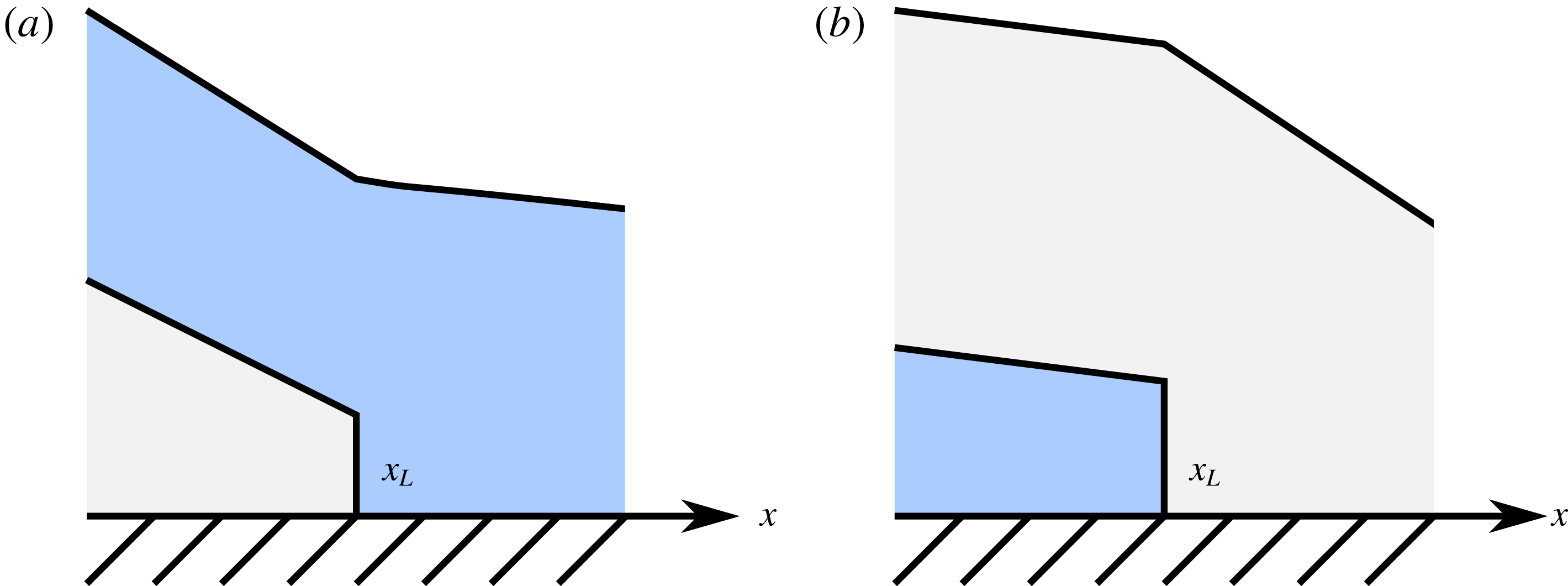
Figure 3. Schematic of (a) stable and (b) unstable flow configurations. Here,
 ${\mathcal{M}}<1$
(the lower layer is more viscous) in (a), whereas
${\mathcal{M}}<1$
(the lower layer is more viscous) in (a), whereas
 ${\mathcal{M}}>1$
(the lower layer is less viscous) in (b).
${\mathcal{M}}>1$
(the lower layer is less viscous) in (b).
4.1 Mechanism of instability
To illustrate the instability mechanism, consider the case
 ${\mathcal{M}}>1$
in which a less viscous fluid intrudes into a more viscous fluid in the unlubricated region, depicted in figure 3(b). In this case, surface slopes, and so pressure gradients, are larger in the unlubricated region than in the lubricated region. If the front is perturbed and the less viscous fluid finds itself in the unlubricated region, it will become subject to higher hydrostatic pressure gradients and so will advance forward, causing an instability. The scenario is reversed in the opposite case
${\mathcal{M}}>1$
in which a less viscous fluid intrudes into a more viscous fluid in the unlubricated region, depicted in figure 3(b). In this case, surface slopes, and so pressure gradients, are larger in the unlubricated region than in the lubricated region. If the front is perturbed and the less viscous fluid finds itself in the unlubricated region, it will become subject to higher hydrostatic pressure gradients and so will advance forward, causing an instability. The scenario is reversed in the opposite case
 ${\mathcal{M}}<1$
, depicted in figure 3(a). In this case, the jump in slope is reversed so that surface slopes, and so pressure gradients, are smaller in the unlubricated region than in the lubricated region, and if the front is perturbed so that the more viscous, underlying fluid gets displaced past the position of the basic-state front, then it will become subject to lower hydrostatic pressure gradients and become suppressed. That is, a viscosity contrast brings with it a change in pressure gradient, which triggers the instability.
${\mathcal{M}}<1$
, depicted in figure 3(a). In this case, the jump in slope is reversed so that surface slopes, and so pressure gradients, are smaller in the unlubricated region than in the lubricated region, and if the front is perturbed so that the more viscous, underlying fluid gets displaced past the position of the basic-state front, then it will become subject to lower hydrostatic pressure gradients and become suppressed. That is, a viscosity contrast brings with it a change in pressure gradient, which triggers the instability.
There is a fundamental similarity between this instability and the Saffman–Taylor instability in that both are caused by discontinuities in a driving pressure gradient. However, in this case, the underlying pressure gradients originate from changes in free-surface slope and are related to hydrostatic pressure rather than dynamic pressure.
We proceed with a formal justification of the physical mechanism in the following sections.
4.2 Perturbations resisted by vertical shear
We use the non-dimensionalisation (2.2), for which we use the length scale
 $$\begin{eqnarray}{\mathcal{L}}=\left(\frac{gq_{0}^{3}T_{0}^{4}}{\unicode[STIX]{x1D708}}\right)^{1/5},\end{eqnarray}$$
where
 $T_{0}$
is the time delay between the initiation of flow of the two layers, as in the experiments of Kowal & Worster (Reference Kowal and Worster2015). The shear-dominated theory of § 2 is supplemented by the following mass conservation equations in the no-slip region (Huppert Reference Huppert1982):
$T_{0}$
is the time delay between the initiation of flow of the two layers, as in the experiments of Kowal & Worster (Reference Kowal and Worster2015). The shear-dominated theory of § 2 is supplemented by the following mass conservation equations in the no-slip region (Huppert Reference Huppert1982):
 $$\begin{eqnarray}\boldsymbol{q}=-\frac{1}{3}H^{3}\unicode[STIX]{x1D735}H,\quad \frac{\unicode[STIX]{x2202}H}{\unicode[STIX]{x2202}t}=-\unicode[STIX]{x1D735}\boldsymbol{\cdot }\boldsymbol{q}\quad (x\geqslant x_{L}),\end{eqnarray}$$
the matching condition
 $$\begin{eqnarray}[H]_{-}^{+}=0\quad (x=x_{L})\end{eqnarray}$$
at the lubrication front, and the flux condition and kinematic condition
 $$\begin{eqnarray}\displaystyle & \displaystyle [\boldsymbol{q}\boldsymbol{\cdot }\boldsymbol{n}_{\boldsymbol{L}}+\boldsymbol{q}_{\boldsymbol{l}}\boldsymbol{\cdot }\boldsymbol{n}_{\boldsymbol{L}}]^{-}=[\boldsymbol{q}\boldsymbol{\cdot }\boldsymbol{n}_{\boldsymbol{L}}]^{+}\quad (x=x_{L}), & \displaystyle\end{eqnarray}$$
 $$\begin{eqnarray}\displaystyle & \displaystyle \boldsymbol{n}_{\boldsymbol{L}}\boldsymbol{\cdot }\dot{\boldsymbol{x}}_{\boldsymbol{L}}=\lim _{x\rightarrow x_{L}}\boldsymbol{n}_{\boldsymbol{L}}\boldsymbol{\cdot }\boldsymbol{q}_{\boldsymbol{l}}/h. & \displaystyle\end{eqnarray}$$
Here, we take
 ${\mathcal{D}}=0$
.
${\mathcal{D}}=0$
.
4.3 Linearisation
We investigate the linear stability of the system by introducing small disturbances of size
 $\unicode[STIX]{x1D716}\ll 1$
(distinct from
$\unicode[STIX]{x1D716}\ll 1$
(distinct from
 $\unicode[STIX]{x1D716}$
used in the previous section) and write
$\unicode[STIX]{x1D716}$
used in the previous section) and write
 $h=h_{0}+\unicode[STIX]{x1D716}h_{1}$
,
$h=h_{0}+\unicode[STIX]{x1D716}h_{1}$
,
 $H=H_{0}+\unicode[STIX]{x1D716}H_{1}$
,
$H=H_{0}+\unicode[STIX]{x1D716}H_{1}$
,
 $x_{L}=x_{L0}+\unicode[STIX]{x1D716}x_{L1}$
and so on. These give rise to the following linearised perturbation fluxes:
$x_{L}=x_{L0}+\unicode[STIX]{x1D716}x_{L1}$
and so on. These give rise to the following linearised perturbation fluxes:
 $$\begin{eqnarray}\boldsymbol{q}_{\boldsymbol{l}\mathbf{1}}=-\left[\left(-\frac{{\mathcal{M}}}{2}h_{0}^{2}h_{1}+{\mathcal{M}}h_{0}h_{1}H_{0}+\frac{{\mathcal{M}}}{2}h_{0}^{2}H_{1}\right)\unicode[STIX]{x1D735}H_{0}+\left(-\frac{{\mathcal{M}}}{6}h_{0}^{3}+\frac{{\mathcal{M}}}{2}h_{0}^{2}H_{0}\right)\unicode[STIX]{x1D735}H_{1}\right],\end{eqnarray}$$
 $$\begin{eqnarray}\displaystyle \boldsymbol{q}_{\mathbf{1}}+\boldsymbol{q}_{\boldsymbol{l}\mathbf{1}} & = & \displaystyle -\left[\vphantom{\left(\frac{1-{\mathcal{M}}}{3}(H_{0}-h_{0})^{3}+\frac{{\mathcal{M}}}{3}H_{0}^{3}\right)}((1-{\mathcal{M}})(H_{0}-h_{0})^{2}(H_{1}-h_{1})+{\mathcal{M}}H_{0}^{2}H_{1})\unicode[STIX]{x1D735}H_{0}\right.\nonumber\\ \displaystyle & & \displaystyle +\left.\left(\frac{1-{\mathcal{M}}}{3}(H_{0}-h_{0})^{3}+\frac{{\mathcal{M}}}{3}H_{0}^{3}\right)\unicode[STIX]{x1D735}H_{1}\right]\end{eqnarray}$$
in the lubricated region and
 $$\begin{eqnarray}\boldsymbol{q}_{\mathbf{1}}=-\left[H_{0}^{2}H_{1}\unicode[STIX]{x1D735}H_{0}+{\textstyle \frac{1}{3}}H_{0}^{3}\unicode[STIX]{x1D735}H_{1}\right]\end{eqnarray}$$
in the unlubricated region. First-order mass conservation equations in the lubricated region are
 $$\begin{eqnarray}\frac{\unicode[STIX]{x2202}h_{1}}{\unicode[STIX]{x2202}t}=-\unicode[STIX]{x1D735}\boldsymbol{\cdot }\boldsymbol{q}_{\boldsymbol{l}\mathbf{1}},\quad \frac{\unicode[STIX]{x2202}(H_{1}-h_{1})}{\unicode[STIX]{x2202}t}=-\unicode[STIX]{x1D735}\boldsymbol{\cdot }\boldsymbol{q}_{\mathbf{1}},\end{eqnarray}$$
and in the unlubricated region
 $$\begin{eqnarray}\frac{\unicode[STIX]{x2202}H_{1}}{\unicode[STIX]{x2202}t}=-\unicode[STIX]{x1D735}\boldsymbol{\cdot }\boldsymbol{q}_{\mathbf{1}}.\end{eqnarray}$$
The condition of flux continuity to first order in
 $\unicode[STIX]{x1D716}$
can be expressed as
$\unicode[STIX]{x1D716}$
can be expressed as
 $$\begin{eqnarray}\left[x_{L1}\frac{\unicode[STIX]{x2202}}{\unicode[STIX]{x2202}x}(\boldsymbol{q}_{\boldsymbol{l}\mathbf{0}}+\boldsymbol{q}_{\mathbf{0}})+(\boldsymbol{q}_{\boldsymbol{l}\mathbf{1}}+\boldsymbol{q}_{\mathbf{1}})\right]^{-}\boldsymbol{\cdot }\boldsymbol{e}_{\boldsymbol{ x}}=\left[x_{L1}\frac{\unicode[STIX]{x2202}}{\unicode[STIX]{x2202}x}\boldsymbol{q}_{\mathbf{0}}+\boldsymbol{q}_{\mathbf{1}}\right]^{+}\boldsymbol{\cdot }\boldsymbol{e}_{\boldsymbol{ x}}\quad (x=x_{L0}).\end{eqnarray}$$
Height continuity to first order gives
 $$\begin{eqnarray}\left[x_{L1}\frac{\unicode[STIX]{x2202}H_{0}}{\unicode[STIX]{x2202}x}+H_{1}\right]^{-}=\left[x_{L1}\frac{\unicode[STIX]{x2202}H_{0}}{\unicode[STIX]{x2202}x}+H_{1}\right]^{+}\quad (x=x_{L0}),\end{eqnarray}$$
and the kinematic condition to first order gives
 $$\begin{eqnarray}{\dot{x}}_{L1}=\frac{1}{h_{0}}\left(x_{L1}\frac{\unicode[STIX]{x2202}\boldsymbol{q}_{\boldsymbol{l}\mathbf{0}}}{\unicode[STIX]{x2202}x}+\boldsymbol{q}_{\boldsymbol{l}\mathbf{1}}\right)\boldsymbol{\cdot }\boldsymbol{e}_{\boldsymbol{x}}-\frac{\boldsymbol{q}_{\boldsymbol{l}\mathbf{0}}\boldsymbol{\cdot }\boldsymbol{e}_{\boldsymbol{x}}}{h_{0}^{2}}\left(x_{L1}\frac{\unicode[STIX]{x2202}h_{0}}{\unicode[STIX]{x2202}x}+h_{1}\right).\end{eqnarray}$$
We wish to perform a local analysis in an inner region of size
 $\unicode[STIX]{x1D6FF}\ll x_{L}$
near the lubrication front in which the surface heights of the two layers in the lubricated region as well as that of the unlubricated region are linear to first order in
$\unicode[STIX]{x1D6FF}\ll x_{L}$
near the lubrication front in which the surface heights of the two layers in the lubricated region as well as that of the unlubricated region are linear to first order in
 $\unicode[STIX]{x1D6FF}$
. This can be attained by rescaling
$\unicode[STIX]{x1D6FF}$
. This can be attained by rescaling
 $$\begin{eqnarray}x-x_{L0}=\unicode[STIX]{x1D6FF}(\tilde{x}-x_{L0}),\quad y=\unicode[STIX]{x1D6FF}{\tilde{y}},\quad t-1=\unicode[STIX]{x1D6FF}^{2}\tilde{t},\end{eqnarray}$$
assuming
 $\tilde{x}$
,
$\tilde{x}$
,
 ${\tilde{y}}$
,
${\tilde{y}}$
,
 $\tilde{t}=\mathit{O}(1)$
as
$\tilde{t}=\mathit{O}(1)$
as
 $\unicode[STIX]{x1D6FF}\rightarrow 0$
, and expanding to first order in
$\unicode[STIX]{x1D6FF}\rightarrow 0$
, and expanding to first order in
 $\unicode[STIX]{x1D6FF}$
. Such an approach can be justified by identifying
$\unicode[STIX]{x1D6FF}$
. Such an approach can be justified by identifying
 $\unicode[STIX]{x1D6FF}$
with
$\unicode[STIX]{x1D6FF}$
with
 $k^{-1}$
. Such an approach also ensures that the linearised quantities are independent of time, which, effectively, imposes a frozen-time approximation. We additionally impose that all perturbations are local to the lubrication front and decay away from it. We present a more detailed analysis involving the full region of the flow and perturbation equations involving the full, space-dependent basic state in the companion paper (Kowal & Worster Reference Kowal and Worster2019).
$k^{-1}$
. Such an approach also ensures that the linearised quantities are independent of time, which, effectively, imposes a frozen-time approximation. We additionally impose that all perturbations are local to the lubrication front and decay away from it. We present a more detailed analysis involving the full region of the flow and perturbation equations involving the full, space-dependent basic state in the companion paper (Kowal & Worster Reference Kowal and Worster2019).
In what follows, we split the domain of the flow into two asymptotic regions: the above-mentioned inner region near the lubrication front, composed of both the lubricated and no-slip domains, and two outer regions away from the lubrication front, which also consist of both the lubricated and no-slip domains.
Evaluating basic-state quantities at
 $t=1$
defines the dimensional time scale
$t=1$
defines the dimensional time scale
 ${\mathcal{T}}$
. We denote the basic-state surface heights in the inner region to first order in
${\mathcal{T}}$
. We denote the basic-state surface heights in the inner region to first order in
 $\unicode[STIX]{x1D6FF}$
by
$\unicode[STIX]{x1D6FF}$
by
 $$\begin{eqnarray}h_{0}=a+b(x-x_{L}),\quad H_{0}=A+B(x-x_{L})\quad (x\leqslant x_{L0})\end{eqnarray}$$
for the lubricated region and
 $$\begin{eqnarray}H_{0}=\unicode[STIX]{x1D6FC}+\unicode[STIX]{x1D6FD}(x-x_{L})\quad (x\geqslant x_{L0})\end{eqnarray}$$
for the unlubricated region, as depicted in the schematic diagram of figure 4.
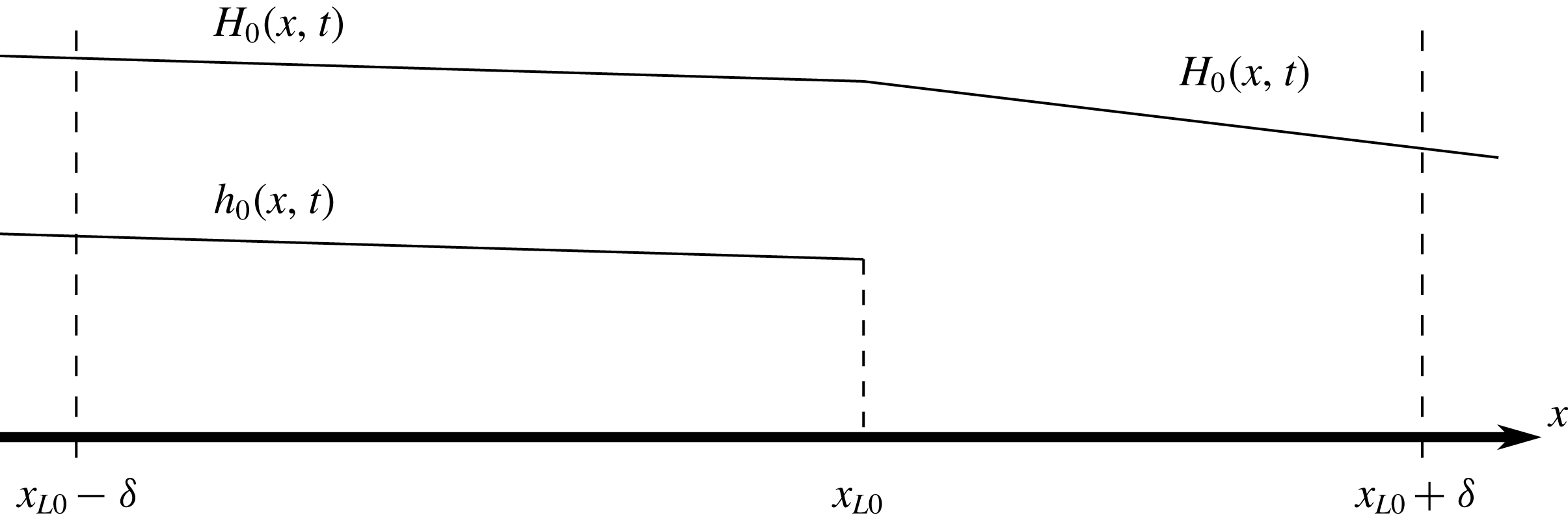
Figure 4. Schematic of the basic state in the inner region, in which the surface heights are locally linear.
By searching for normal-mode solutions in the frame of the lubrication front and writing
 $$\begin{eqnarray}(h_{1}(x,y,t),H_{1}(x,y,t),x_{L1}(y,t))=({\hat{h}}_{1}(x),{\hat{H}}_{1}(x),\hat{x}_{L1})\exp (\unicode[STIX]{x1D70E}t+\text{i}ky),\end{eqnarray}$$
where
 $k$
is the transverse wavenumber of the disturbances and
$k$
is the transverse wavenumber of the disturbances and
 $\unicode[STIX]{x1D70E}$
is their (complex) growth rate, we find that the amplitudes satisfy the following mass conservation equations (after dropping hats):
$\unicode[STIX]{x1D70E}$
is their (complex) growth rate, we find that the amplitudes satisfy the following mass conservation equations (after dropping hats):
 $$\begin{eqnarray}\displaystyle & \unicode[STIX]{x1D70E}h_{1}-Vh_{1}^{\prime }=(a_{l1}H_{0}^{\prime }+a_{l2}H_{1}^{\prime })^{\prime }-a_{l3}k^{2}H_{1}\quad (x\leqslant x_{L0}), & \displaystyle\end{eqnarray}$$
 $$\begin{eqnarray}\displaystyle & \unicode[STIX]{x1D70E}H_{1}-VH_{1}^{\prime }=(a_{1}H_{0}^{\prime }+a_{2}H_{1}^{\prime })^{\prime }-a_{3}k^{2}H_{1}\quad (x\leqslant x_{L0}) & \displaystyle\end{eqnarray}$$
for the lubricated region and
 $$\begin{eqnarray}\unicode[STIX]{x1D70E}H_{1}-VH_{1}^{\prime }=\left[H_{0}^{2}H_{1}H_{0}^{\prime }+\frac{1}{3}H_{0}^{3}H_{1}^{\prime }\right]^{\prime }-\frac{k^{2}}{3}H_{0}^{3}H_{1}\quad (x\geqslant x_{L0})\end{eqnarray}$$
for the unlubricated region, where
 $a_{li},a_{i}$
, for
$a_{li},a_{i}$
, for
 $i=1,\ldots ,3$
, are cubic functions of the basic-state layer thicknesses and the viscosity ratio
$i=1,\ldots ,3$
, are cubic functions of the basic-state layer thicknesses and the viscosity ratio
 ${\mathcal{M}}$
, which are given in (S.1)–(S.9) of the supplementary material available at https://doi.org/10.1017/jfm.2019.321. Here,
${\mathcal{M}}$
, which are given in (S.1)–(S.9) of the supplementary material available at https://doi.org/10.1017/jfm.2019.321. Here,
 $V={\dot{x}}_{L0}$
is the velocity of the lubrication front, which is related to
$V={\dot{x}}_{L0}$
is the velocity of the lubrication front, which is related to
 $A$
,
$A$
,
 $B$
,
$B$
,
 $a$
and
$a$
and
 $b$
through its dependence on the three dimensionless parameters. Of interest to us are the equations (4.18)–(4.20) up to first order in
$b$
through its dependence on the three dimensionless parameters. Of interest to us are the equations (4.18)–(4.20) up to first order in
 $\unicode[STIX]{x1D6FF}$
(see (D 1)–(D 3) of appendix D for details).
$\unicode[STIX]{x1D6FF}$
(see (D 1)–(D 3) of appendix D for details).
The first-order flux continuity boundary condition reduces to
 $$\begin{eqnarray}\left\{\bar{c}_{1}x_{L1}+\bar{c}_{2}H_{1}+\bar{c}_{3}h_{1}+\bar{c}_{4}\frac{\unicode[STIX]{x2202}H_{1}}{\unicode[STIX]{x2202}x}\right\}^{-}=\left\{x_{L1}\unicode[STIX]{x1D6FC}^{2}\unicode[STIX]{x1D6FD}^{2}+\unicode[STIX]{x1D6FC}^{2}\unicode[STIX]{x1D6FD}H_{1}+\frac{1}{3}\unicode[STIX]{x1D6FC}^{3}\frac{\unicode[STIX]{x2202}H_{1}}{\unicode[STIX]{x2202}x}\right\}^{+}\end{eqnarray}$$
for
 $x=x_{L0}$
, where
$x=x_{L0}$
, where
 $\bar{c}_{1},\ldots ,\bar{c}_{4}$
are functions of the viscosity ratio
$\bar{c}_{1},\ldots ,\bar{c}_{4}$
are functions of the viscosity ratio
 ${\mathcal{M}}$
, the basic-state thicknesses
${\mathcal{M}}$
, the basic-state thicknesses
 $a,A$
and slopes
$a,A$
and slopes
 $b,B$
, and are given in (S.43)–(S.46) of the supplementary material. Similarly, the condition for continuity of height becomes
$b,B$
, and are given in (S.43)–(S.46) of the supplementary material. Similarly, the condition for continuity of height becomes
 $$\begin{eqnarray}[x_{L1}B+H_{1}]^{-}=[x_{L1}\unicode[STIX]{x1D6FD}+H_{1}]^{+}\end{eqnarray}$$
for
 $x=x_{L0}$
. The kinematic condition becomes
$x=x_{L0}$
. The kinematic condition becomes
 $$\begin{eqnarray}\unicode[STIX]{x1D70E}x_{L1}={\mathcal{M}}\left(c_{8}x_{L1}+c_{9}h_{1}+c_{10}H_{1}+c_{11}\frac{\unicode[STIX]{x2202}H_{1}}{\unicode[STIX]{x2202}x}\right)\end{eqnarray}$$
for
 $x=x_{L0}^{-}$
, where
$x=x_{L0}^{-}$
, where
 $c_{8},\ldots ,c_{11}$
are functions of the layer thicknesses and their derivatives, and are given in (S.47)–(S.50) of the supplementary material.
$c_{8},\ldots ,c_{11}$
are functions of the layer thicknesses and their derivatives, and are given in (S.47)–(S.50) of the supplementary material.
The equations (4.18)–(4.20) up to first order in
 $\unicode[STIX]{x1D6FF}$
along with the boundary conditions (4.21)–(4.23) form a system of linear differential equations with constant coefficients, with solutions of the form
$\unicode[STIX]{x1D6FF}$
along with the boundary conditions (4.21)–(4.23) form a system of linear differential equations with constant coefficients, with solutions of the form
 $$\begin{eqnarray}\displaystyle & (h_{1},H_{1})=(\tilde{h}_{1}^{-},\tilde{H}_{1}^{-})\exp ((x-x_{L0})\unicode[STIX]{x1D706}^{-})\quad (x\leqslant x_{L0}), & \displaystyle\end{eqnarray}$$
 $$\begin{eqnarray}\displaystyle & H_{1}=\tilde{H}_{1}^{+}\exp ((x-x_{L0})\unicode[STIX]{x1D706}^{+})\quad (x\geqslant x_{L0}), & \displaystyle\end{eqnarray}$$
 $\tilde{h}_{1}^{-}$
,
$\tilde{h}_{1}^{-}$
,
 $\tilde{H}_{1}^{-}$
and
$\tilde{H}_{1}^{-}$
and
 $\tilde{H}_{1}^{+}$
are constants. Direct substitution into the mass conservation equations (D 1)–(D 3) and corresponding matching conditions yields a system of six algebraic equations for the six unknown variables
$\tilde{H}_{1}^{+}$
are constants. Direct substitution into the mass conservation equations (D 1)–(D 3) and corresponding matching conditions yields a system of six algebraic equations for the six unknown variables
 $\unicode[STIX]{x1D70E}$
,
$\unicode[STIX]{x1D70E}$
,
 $x_{L1}$
,
$x_{L1}$
,
 $\tilde{h}_{1}^{-}$
,
$\tilde{h}_{1}^{-}$
,
 $\tilde{H}_{1}^{+}$
,
$\tilde{H}_{1}^{+}$
,
 $\unicode[STIX]{x1D706}^{-}$
and
$\unicode[STIX]{x1D706}^{-}$
and
 $\unicode[STIX]{x1D706}^{+}$
, where it has been assumed that
$\unicode[STIX]{x1D706}^{+}$
, where it has been assumed that
 $\tilde{H}_{1}^{-}\equiv 1$
, without loss of generality, as solutions of this eigenproblem are defined only up to a multiplicative constant. We restrict the choice of solutions to those that decay exponentially from the lubrication front, giving that
$\tilde{H}_{1}^{-}\equiv 1$
, without loss of generality, as solutions of this eigenproblem are defined only up to a multiplicative constant. We restrict the choice of solutions to those that decay exponentially from the lubrication front, giving that
 $\unicode[STIX]{x1D706}^{-}>0$
and
$\unicode[STIX]{x1D706}^{-}>0$
and
 $\unicode[STIX]{x1D706}^{+}<0$
.
$\unicode[STIX]{x1D706}^{+}<0$
.Expressing the mass conservation equations in the lubricated region in matrix form gives
 $$\begin{eqnarray}(\unicode[STIX]{x1D64B}-(\unicode[STIX]{x1D70E}-V\unicode[STIX]{x1D706}^{-})\unicode[STIX]{x1D644})[\tilde{h}_{1}^{-},\tilde{H}_{1}^{-}]^{\text{T}}=\mathbf{0},\end{eqnarray}$$
where
 $\unicode[STIX]{x1D64B}$
is a
$\unicode[STIX]{x1D64B}$
is a
 $2\times 2$
matrix with entries that are a function of
$2\times 2$
matrix with entries that are a function of
 $\unicode[STIX]{x1D706}^{-}$
,
$\unicode[STIX]{x1D706}^{-}$
,
 $k$
,
$k$
,
 $a,A,b,B$
and
$a,A,b,B$
and
 ${\mathcal{M}}$
. The entries of
${\mathcal{M}}$
. The entries of
 $\unicode[STIX]{x1D64B}$
are given explicitly in (S.51)–(S.54) of the supplementary material. Requiring non-trivial solutions gives that
$\unicode[STIX]{x1D64B}$
are given explicitly in (S.51)–(S.54) of the supplementary material. Requiring non-trivial solutions gives that
 $\unicode[STIX]{x1D706}^{-}$
satisfies
$\unicode[STIX]{x1D706}^{-}$
satisfies
 $$\begin{eqnarray}\det (\unicode[STIX]{x1D64B}-(\unicode[STIX]{x1D70E}-V\unicode[STIX]{x1D706}^{-})\unicode[STIX]{x1D644})=0,\end{eqnarray}$$
which is a cubic equation for
 $\unicode[STIX]{x1D706}^{-}$
. Recalling that
$\unicode[STIX]{x1D706}^{-}$
. Recalling that
 $\tilde{H}_{1}^{-}=1$
, without loss of generality, it follows that
$\tilde{H}_{1}^{-}=1$
, without loss of generality, it follows that
 $\tilde{h}_{1}^{-}$
is given by the corresponding solution to (4.26), that is,
$\tilde{h}_{1}^{-}$
is given by the corresponding solution to (4.26), that is,
 $$\begin{eqnarray}\tilde{h}_{1}^{-}=\frac{(a(b(6B-3a\unicode[STIX]{x1D706}^{-}+6A\unicode[STIX]{x1D706}^{-})+a(6B\unicode[STIX]{x1D706}^{-}+(a-3A)(k-\unicode[STIX]{x1D706}^{-})(k+\unicode[STIX]{x1D706}^{-}))){\mathcal{M}})}{(3B(-2Ab+a^{2}\unicode[STIX]{x1D706}^{-}+2a(b-B-A\unicode[STIX]{x1D706}^{-})){\mathcal{M}}+6\unicode[STIX]{x1D70E}-6V\unicode[STIX]{x1D706}^{-})}.\end{eqnarray}$$
Solving the mass conservation equation within the unlubricated region subject to decay conditions gives
 $\unicode[STIX]{x1D706}^{+}$
explicitly as
$\unicode[STIX]{x1D706}^{+}$
explicitly as
 $$\begin{eqnarray}\unicode[STIX]{x1D706}^{+}=-\frac{1}{2\unicode[STIX]{x1D6FC}^{3}}(6\unicode[STIX]{x1D6FC}^{2}\unicode[STIX]{x1D6FD}+3V+\sqrt{4\unicode[STIX]{x1D6FC}^{3}(3\unicode[STIX]{x1D6FC}\unicode[STIX]{x1D6FD}^{2}+\unicode[STIX]{x1D6FC}^{3}k^{2}+3\unicode[STIX]{x1D70E})+36\unicode[STIX]{x1D6FC}^{2}\unicode[STIX]{x1D6FD}V+9V^{2}}).\end{eqnarray}$$
The flux continuity condition specifies the dispersion relation for
 $\unicode[STIX]{x1D70E}$
in the form
$\unicode[STIX]{x1D70E}$
in the form
 $$\begin{eqnarray}\unicode[STIX]{x1D701}_{1}x_{L1}+\unicode[STIX]{x1D701}_{2}\tilde{H}_{1}^{-}+\unicode[STIX]{x1D701}_{3}\tilde{h}_{1}^{-}=-{\textstyle \frac{1}{3}}\unicode[STIX]{x1D6FC}^{2}(3\unicode[STIX]{x1D6FD}\tilde{H}_{1}^{+}+\unicode[STIX]{x1D6FC}\tilde{H}_{1}^{+}\unicode[STIX]{x1D706}^{+}+3\unicode[STIX]{x1D6FD}^{2}x_{L1}),\end{eqnarray}$$
where
 $\unicode[STIX]{x1D701}_{1},\ldots ,\unicode[STIX]{x1D701}_{3}$
are functions of
$\unicode[STIX]{x1D701}_{1},\ldots ,\unicode[STIX]{x1D701}_{3}$
are functions of
 $a,A,b,B,{\mathcal{M}}$
and
$a,A,b,B,{\mathcal{M}}$
and
 $\unicode[STIX]{x1D706}^{-}$
and are given in (S.55)–(S.57) of the supplementary material. This is an implicit equation for
$\unicode[STIX]{x1D706}^{-}$
and are given in (S.55)–(S.57) of the supplementary material. This is an implicit equation for
 $\unicode[STIX]{x1D70E}$
, which appears via
$\unicode[STIX]{x1D70E}$
, which appears via
 $\unicode[STIX]{x1D706}^{-}$
and
$\unicode[STIX]{x1D706}^{-}$
and
 $\unicode[STIX]{x1D706}^{+}$
. The
$\unicode[STIX]{x1D706}^{+}$
. The
 $\unicode[STIX]{x1D706}^{-}$
and
$\unicode[STIX]{x1D706}^{-}$
and
 $\unicode[STIX]{x1D706}^{+}$
appear linearly in the dispersion relation and are solutions of cubic and quadratic equations, respectively. More than one solution for
$\unicode[STIX]{x1D706}^{+}$
appear linearly in the dispersion relation and are solutions of cubic and quadratic equations, respectively. More than one solution for
 $\unicode[STIX]{x1D706}^{-}$
and
$\unicode[STIX]{x1D706}^{-}$
and
 $\unicode[STIX]{x1D706}^{+}$
, and hence for
$\unicode[STIX]{x1D706}^{+}$
, and hence for
 $\unicode[STIX]{x1D70E}$
, are possible and we are interested in the solution for which the real part of
$\unicode[STIX]{x1D70E}$
, are possible and we are interested in the solution for which the real part of
 $\unicode[STIX]{x1D70E}$
is largest. Parameters
$\unicode[STIX]{x1D70E}$
is largest. Parameters
 $\tilde{H}_{1}^{+}$
and
$\tilde{H}_{1}^{+}$
and
 $x_{L1}$
are found by using the height continuity and kinematic conditions to be
$x_{L1}$
are found by using the height continuity and kinematic conditions to be
 $$\begin{eqnarray}\tilde{H}_{1}^{+}=x_{L1}(B-\unicode[STIX]{x1D6FD})+\tilde{H}_{1}^{-}\end{eqnarray}$$
and
 $$\begin{eqnarray}x_{L1}=\frac{1}{\unicode[STIX]{x1D701}_{6}}(\unicode[STIX]{x1D701}_{4}\tilde{h}_{1}^{-}+\unicode[STIX]{x1D701}_{5}\tilde{H}_{1}^{-}),\end{eqnarray}$$
where
 $\unicode[STIX]{x1D701}_{4},\ldots ,\unicode[STIX]{x1D701}_{6}$
are functions of
$\unicode[STIX]{x1D701}_{4},\ldots ,\unicode[STIX]{x1D701}_{6}$
are functions of
 $a,A,b,B,{\mathcal{M}},\unicode[STIX]{x1D70E}$
and
$a,A,b,B,{\mathcal{M}},\unicode[STIX]{x1D70E}$
and
 $\unicode[STIX]{x1D706}^{-}$
and are given in (S.58)–(S.60) of the supplementary material.
$\unicode[STIX]{x1D706}^{-}$
and are given in (S.58)–(S.60) of the supplementary material.
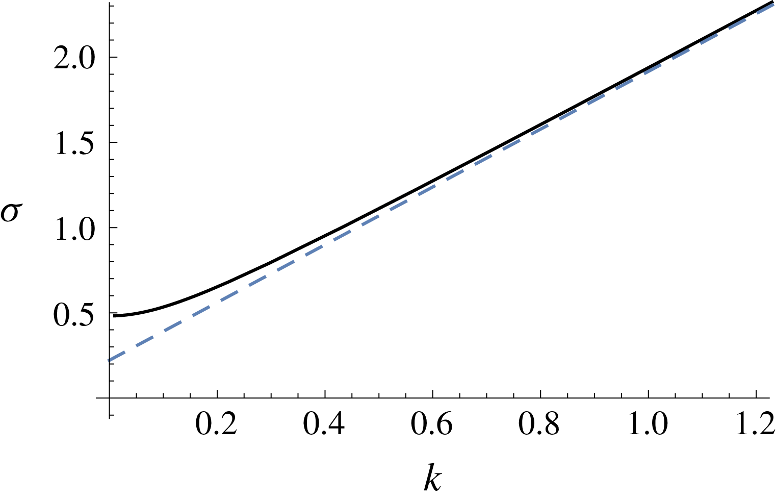
Figure 5. Asymptotic (dashed) and numerical (solid) solutions of the equations of § 4 for the growth rates
 $\unicode[STIX]{x1D70E}$
against wavenumber
$\unicode[STIX]{x1D70E}$
against wavenumber
 $k$
for perturbations resisted dominantly by vertical shear. Parameter values used are
$k$
for perturbations resisted dominantly by vertical shear. Parameter values used are
 ${\mathcal{M}}=10$
and
${\mathcal{M}}=10$
and
 ${\mathcal{Q}}=0.1$
.
${\mathcal{Q}}=0.1$
.
In this section, we have determined the dispersion relation for
 $\unicode[STIX]{x1D70E}$
in terms of quantities such as the perturbations to the surface heights and leading edge position. Equations in this section are solved numerically and the solutions for
$\unicode[STIX]{x1D70E}$
in terms of quantities such as the perturbations to the surface heights and leading edge position. Equations in this section are solved numerically and the solutions for
 $\unicode[STIX]{x1D70E}$
are shown in figure 5. In order to formulate a stability criterion, we simplify these using large-wavenumber asymptotics in the following section.
$\unicode[STIX]{x1D70E}$
are shown in figure 5. In order to formulate a stability criterion, we simplify these using large-wavenumber asymptotics in the following section.
4.4 Large-
 $k$
asymptotics
$k$
asymptotics

In what follows, we expand in series of
 $1/k$
for
$1/k$
for
 $k$
large and write
$k$
large and write
 $X=X_{0}k+X_{1}+\cdots \,$
, where
$X=X_{0}k+X_{1}+\cdots \,$
, where
 $X=(\unicode[STIX]{x1D70E},\unicode[STIX]{x1D706}^{\pm },\tilde{H}_{1}^{\pm },\tilde{h}_{1}^{-},x_{L1})$
. Using (4.26) gives the leading-order governing equation in the lubricated region
$X=(\unicode[STIX]{x1D70E},\unicode[STIX]{x1D706}^{\pm },\tilde{H}_{1}^{\pm },\tilde{h}_{1}^{-},x_{L1})$
. Using (4.26) gives the leading-order governing equation in the lubricated region
 $$\begin{eqnarray}{\textstyle \frac{1}{6}}k^{3}[(\unicode[STIX]{x1D706}_{0}^{-})^{2}-1][\unicode[STIX]{x1D706}_{0}^{-}-\tilde{\unicode[STIX]{x1D706}}_{0}^{-}]=O(k^{2})\end{eqnarray}$$
giving
 $\unicode[STIX]{x1D706}_{0}^{-}=\pm 1$
or
$\unicode[STIX]{x1D706}_{0}^{-}=\pm 1$
or
 $\unicode[STIX]{x1D706}_{0}^{-}=\tilde{\unicode[STIX]{x1D706}}_{0}^{-}$
, where
$\unicode[STIX]{x1D706}_{0}^{-}=\tilde{\unicode[STIX]{x1D706}}_{0}^{-}$
, where
 $$\begin{eqnarray}\tilde{\unicode[STIX]{x1D706}}_{0}^{-}=-\frac{2\unicode[STIX]{x1D70E}_{0}\tilde{\unicode[STIX]{x1D706}}_{n0}}{\tilde{\unicode[STIX]{x1D706}}_{d0}}\end{eqnarray}$$
and
 $\tilde{\unicode[STIX]{x1D706}}_{n0},\tilde{\unicode[STIX]{x1D706}}_{d0}$
are functions of the layer thicknesses, slopes, viscosity ratio
$\tilde{\unicode[STIX]{x1D706}}_{n0},\tilde{\unicode[STIX]{x1D706}}_{d0}$
are functions of the layer thicknesses, slopes, viscosity ratio
 ${\mathcal{M}}$
and
${\mathcal{M}}$
and
 $V$
. Explicit expressions are given in (S.61)–(S.62) of the supplementary material. It can be deduced from the latter expression that
$V$
. Explicit expressions are given in (S.61)–(S.62) of the supplementary material. It can be deduced from the latter expression that
 $\tilde{\unicode[STIX]{x1D706}}_{0}^{-}\rightarrow 0$
as
$\tilde{\unicode[STIX]{x1D706}}_{0}^{-}\rightarrow 0$
as
 ${\mathcal{M}}\rightarrow 0$
. Taking
${\mathcal{M}}\rightarrow 0$
. Taking
 $\unicode[STIX]{x1D706}_{0}^{-}=1$
gives the next-order equation outlined in the supplementary material, which gives the next-order contribution
$\unicode[STIX]{x1D706}_{0}^{-}=1$
gives the next-order equation outlined in the supplementary material, which gives the next-order contribution
 $$\begin{eqnarray}\unicode[STIX]{x1D706}_{1}^{-}=\frac{\unicode[STIX]{x1D706}_{n1}^{-}}{\unicode[STIX]{x1D706}_{d1}^{-}},\end{eqnarray}$$
where
 $\unicode[STIX]{x1D706}_{n1}^{-},\unicode[STIX]{x1D706}_{d1}^{-}$
are given in (S.64)–(S.65) of the supplementary material. The relation (4.27) between
$\unicode[STIX]{x1D706}_{n1}^{-},\unicode[STIX]{x1D706}_{d1}^{-}$
are given in (S.64)–(S.65) of the supplementary material. The relation (4.27) between
 $\tilde{h}_{1}^{-}$
and
$\tilde{h}_{1}^{-}$
and
 $\tilde{H}_{1}^{-}$
, given without loss of generality that
$\tilde{H}_{1}^{-}$
, given without loss of generality that
 $\tilde{H}_{0}^{-}=1$
, yields
$\tilde{H}_{0}^{-}=1$
, yields
 $$\begin{eqnarray}\tilde{h}_{10}^{-}k+\tilde{h}_{11}^{-}+O(1/k)=\frac{\unicode[STIX]{x1D701}_{7}}{\unicode[STIX]{x1D701}_{8}},\end{eqnarray}$$
where
 $\unicode[STIX]{x1D701}_{7},\unicode[STIX]{x1D701}_{8}$
are given in (S.66)–(S.67) of the supplementary material. Here
$\unicode[STIX]{x1D701}_{7},\unicode[STIX]{x1D701}_{8}$
are given in (S.66)–(S.67) of the supplementary material. Here
 $\unicode[STIX]{x1D701}_{7},\unicode[STIX]{x1D701}_{8}$
are functions of
$\unicode[STIX]{x1D701}_{7},\unicode[STIX]{x1D701}_{8}$
are functions of
 $k$
, among other quantities. Expanding in series of
$k$
, among other quantities. Expanding in series of
 $1/k$
gives that
$1/k$
gives that
 $\tilde{h}_{10}^{-}=0$
and
$\tilde{h}_{10}^{-}=0$
and
 $$\begin{eqnarray}\tilde{h}_{11}^{-}=\left[\frac{a{\mathcal{M}}(6Ab-2a^{2}\unicode[STIX]{x1D706}_{1}^{-}+a(-3b+6(B+A\unicode[STIX]{x1D706}_{1}^{-})))}{3a(a-2A)B{\mathcal{M}}+6(\unicode[STIX]{x1D70E}_{0}-V)}\right].\end{eqnarray}$$
The governing equation (4.28) for the unlubricated region gives that
 $$\begin{eqnarray}\displaystyle \unicode[STIX]{x1D706}_{0}^{+}k+\unicode[STIX]{x1D706}_{1}^{+}O(1/k) & = & \displaystyle \frac{1}{2}\left[-\frac{6\unicode[STIX]{x1D6FD}}{\unicode[STIX]{x1D6FC}}-\frac{3V}{\unicode[STIX]{x1D6FC}^{3}}-\sqrt{4\unicode[STIX]{x1D6FC}^{6}k^{2}+12\unicode[STIX]{x1D6FC}^{3}\unicode[STIX]{x1D70E}_{0}k+O(1)}\right]\nonumber\\ \displaystyle & = & \displaystyle -k-\frac{3}{2}\left[2\frac{\unicode[STIX]{x1D6FD}}{\unicode[STIX]{x1D6FC}}+\frac{\unicode[STIX]{x1D70E}_{0}+V\unicode[STIX]{x1D706}^{+}}{\unicode[STIX]{x1D6FC}^{3}}\right]+O(1/k),\end{eqnarray}$$
and so
 $\unicode[STIX]{x1D706}_{0}^{+}=-1$
and
$\unicode[STIX]{x1D706}_{0}^{+}=-1$
and
 $\unicode[STIX]{x1D706}_{1}^{+}=-(3/2)[2(\unicode[STIX]{x1D6FD}/\unicode[STIX]{x1D6FC})+((\unicode[STIX]{x1D70E}_{0}+V\unicode[STIX]{x1D706}^{+})/\unicode[STIX]{x1D6FC}^{3})]$
. The kinematic condition gives that
$\unicode[STIX]{x1D706}_{1}^{+}=-(3/2)[2(\unicode[STIX]{x1D6FD}/\unicode[STIX]{x1D6FC})+((\unicode[STIX]{x1D70E}_{0}+V\unicode[STIX]{x1D706}^{+})/\unicode[STIX]{x1D6FC}^{3})]$
. The kinematic condition gives that
 $$\begin{eqnarray}\displaystyle & \displaystyle x_{L10}=0, & \displaystyle\end{eqnarray}$$
 $$\begin{eqnarray}\displaystyle & \displaystyle x_{L11}=-\frac{2(A-a)^{3}+3a(2A-a)(A-a)\{}{6a\unicode[STIX]{x1D70E}_{0}}. & \displaystyle\end{eqnarray}$$
The next-order contribution,
 $x_{L12}$
, which will be needed in determining the first-order correction to the dispersion relation (note
$x_{L12}$
, which will be needed in determining the first-order correction to the dispersion relation (note
 $x_{L11}$
was needed in determining the dispersion relation at leading order), is given in (S.68) of the supplementary material. The height continuity condition gives
$x_{L11}$
was needed in determining the dispersion relation at leading order), is given in (S.68) of the supplementary material. The height continuity condition gives
 $$\begin{eqnarray}\displaystyle \tilde{H}^{+} & = & \displaystyle x_{L1}(B-\unicode[STIX]{x1D6FD})+\tilde{H}^{-}\nonumber\\ \displaystyle & = & \displaystyle x_{L11}(B-\unicode[STIX]{x1D6FD})+\tilde{H}_{11}^{-}+x_{L12}(B-\unicode[STIX]{x1D6FD})\frac{1}{k}+O(1/k^{2})\end{eqnarray}$$
and so
 $$\begin{eqnarray}\tilde{H}_{10}^{+}=0,\quad \tilde{H}_{11}^{+}=x_{L11}(B-\unicode[STIX]{x1D6FD})+\tilde{H}_{11}^{-},\quad \tilde{H}_{12}^{+}=x_{L12}(B-\unicode[STIX]{x1D6FD}).\end{eqnarray}$$
The leading-order flux condition reduces to
 $$\begin{eqnarray}\tilde{H}_{11}^{+}=[(1-{\mathcal{M}})(1-a/A)^{3}+{\mathcal{M}}]\frac{\tilde{H}_{11}^{-}}{\unicode[STIX]{x1D706}_{0}^{+}},\end{eqnarray}$$
which, by comparison to (4.41b ), gives
 $$\begin{eqnarray}\unicode[STIX]{x1D70E}_{0}=\unicode[STIX]{x1D6FE}(a,A,{\mathcal{M}})(B-\unicode[STIX]{x1D6FD}),\end{eqnarray}$$
where
 $$\begin{eqnarray}\unicode[STIX]{x1D6FE}(a,A,{\mathcal{M}})=\frac{A-a}{6a}\cdot \frac{2(A-a)^{2}+3a(2A-a){\mathcal{M}}}{({\mathcal{M}}+1)+(1-a/A)^{3}(1-{\mathcal{M}})}.\end{eqnarray}$$
4.5 Instability threshold
The formula (4.43) shows that to leading order, the growth rate behaves as
 $$\begin{eqnarray}\unicode[STIX]{x1D70E}\sim -k\unicode[STIX]{x1D6FE}(a,A,{\mathcal{M}})\left[\frac{\unicode[STIX]{x2202}H_{0}}{\unicode[STIX]{x2202}x}\right]_{-}^{+},\end{eqnarray}$$
at
 $x=x_{L0}$
, as
$x=x_{L0}$
, as
 $k\rightarrow \infty$
. That is, the growth rate varies linearly with
$k\rightarrow \infty$
. That is, the growth rate varies linearly with
 $k$
, as
$k$
, as
 $k\rightarrow \infty$
, which signifies that there is no stabilising mechanism at large wavenumbers under the physics considered so far, similarly to the original result of Saffman & Taylor (Reference Saffman and Taylor1958) for the onset of viscous fingering in a porous medium without the stabilising influence of surface tension. We explore possible stabilising mechanisms in §§ 5 and 6 of this paper and in the companion paper. Since
$k\rightarrow \infty$
, which signifies that there is no stabilising mechanism at large wavenumbers under the physics considered so far, similarly to the original result of Saffman & Taylor (Reference Saffman and Taylor1958) for the onset of viscous fingering in a porous medium without the stabilising influence of surface tension. We explore possible stabilising mechanisms in §§ 5 and 6 of this paper and in the companion paper. Since
 $\unicode[STIX]{x1D6FE}(a,A,{\mathcal{M}})$
in this expression is a positive constant, one can deduce that there are positive growth rates at large wavenumbers precisely when
$\unicode[STIX]{x1D6FE}(a,A,{\mathcal{M}})$
in this expression is a positive constant, one can deduce that there are positive growth rates at large wavenumbers precisely when
 $$\begin{eqnarray}\frac{\unicode[STIX]{x2202}H_{0}}{\unicode[STIX]{x2202}x}^{-}>\frac{\unicode[STIX]{x2202}H_{0}}{\unicode[STIX]{x2202}x}^{+}\quad (x=x_{L0}),\end{eqnarray}$$
that is, when the upper surface slope is gentler in the lubricated region than in the unlubricated region:
 $|\unicode[STIX]{x2202}H_{0}^{-}/\unicode[STIX]{x2202}x|<|\unicode[STIX]{x2202}H_{0}^{+}/\unicode[STIX]{x2202}x|$
, since the surface slopes are negative.
$|\unicode[STIX]{x2202}H_{0}^{-}/\unicode[STIX]{x2202}x|<|\unicode[STIX]{x2202}H_{0}^{+}/\unicode[STIX]{x2202}x|$
, since the surface slopes are negative.
To understand the conditions under which precisely this break in slope occurs, the condition of continuity of flux for the basic state
 $(\boldsymbol{q}_{\mathbf{0}}+\boldsymbol{q}_{\boldsymbol{l}\mathbf{0}})^{-}\boldsymbol{\cdot }\boldsymbol{e}_{\boldsymbol{x}}=\boldsymbol{q}_{\mathbf{0}}^{+}\boldsymbol{\cdot }\boldsymbol{e}_{\boldsymbol{x}}$
, written explicitly as
$(\boldsymbol{q}_{\mathbf{0}}+\boldsymbol{q}_{\boldsymbol{l}\mathbf{0}})^{-}\boldsymbol{\cdot }\boldsymbol{e}_{\boldsymbol{x}}=\boldsymbol{q}_{\mathbf{0}}^{+}\boldsymbol{\cdot }\boldsymbol{e}_{\boldsymbol{x}}$
, written explicitly as
 $$\begin{eqnarray}\left\{-\frac{1}{3}[(1-{\mathcal{M}})(H_{0}-h_{0})^{3}+{\mathcal{M}}H_{0}^{3}]\frac{\unicode[STIX]{x2202}H_{0}}{\unicode[STIX]{x2202}x}\right\}^{-}=\left\{-\frac{1}{3}H_{0}^{3}\frac{\unicode[STIX]{x2202}H_{0}}{\unicode[STIX]{x2202}x}\right\}^{+},\end{eqnarray}$$
may be used to relate the upstream and downstream upper surface slopes as
 $$\begin{eqnarray}\unicode[STIX]{x1D6FD}=[(1-{\mathcal{M}})(1-a/A)^{3}+{\mathcal{M}}]B,\end{eqnarray}$$
showing that
 $B$
and
$B$
and
 $\unicode[STIX]{x1D6FD}$
have the same sign (negative), since the prefactor on the right-hand side is positive, and that the condition
$\unicode[STIX]{x1D6FD}$
have the same sign (negative), since the prefactor on the right-hand side is positive, and that the condition
 $B>\unicode[STIX]{x1D6FD}$
is equivalent to
$B>\unicode[STIX]{x1D6FD}$
is equivalent to
 $$\begin{eqnarray}[(1-{\mathcal{M}})(1-a/A)^{3}+{\mathcal{M}}]>1,\end{eqnarray}$$
that is,
 $$\begin{eqnarray}({\mathcal{M}}-1)[1-(1-a/A)^{3}]>0,\end{eqnarray}$$
or, equivalently,
 $$\begin{eqnarray}{\mathcal{M}}>1.\end{eqnarray}$$
Therefore, the jump in slope is completely determined by the viscosity ratio between the two fluids, which further determines the stability of the front at large wavenumbers.
4.6 Higher-order contributions
In order to determine an asymptotic solution, such that the difference between it and the full numerical solution decays to zero as
 $k\rightarrow \infty$
, we examine the next order. This provides visual agreement between asymptotic and numerical results for moderate wavenumbers. To the next order, the flux condition gives
$k\rightarrow \infty$
, we examine the next order. This provides visual agreement between asymptotic and numerical results for moderate wavenumbers. To the next order, the flux condition gives
 $$\begin{eqnarray}\tilde{H}_{12}^{+}=\unicode[STIX]{x1D719}_{1}\tilde{h}_{11}^{-}+\unicode[STIX]{x1D719}_{2}\tilde{H}_{11}^{-}+\unicode[STIX]{x1D719}_{3}\tilde{H}_{11}^{+}+\unicode[STIX]{x1D719}_{4}x_{L11},\end{eqnarray}$$
where
 $\unicode[STIX]{x1D719}_{1},\ldots ,\unicode[STIX]{x1D719}_{4}$
are given in (S.69)–(S.72) of the supplementary material. Relating this to (4.41c
) gives the next-order correction for the growth rate
$\unicode[STIX]{x1D719}_{1},\ldots ,\unicode[STIX]{x1D719}_{4}$
are given in (S.69)–(S.72) of the supplementary material. Relating this to (4.41c
) gives the next-order correction for the growth rate
 $$\begin{eqnarray}\unicode[STIX]{x1D70E}_{1}=\unicode[STIX]{x1D719}_{5}\tilde{h}_{11}^{-}+\unicode[STIX]{x1D719}_{6}\tilde{H}_{11}^{-}+\unicode[STIX]{x1D719}_{7}\tilde{H}_{11}^{+}+\unicode[STIX]{x1D719}_{8}x_{L11},\end{eqnarray}$$
where the coefficients
 $\unicode[STIX]{x1D719}_{5},\ldots ,\unicode[STIX]{x1D719}_{8}$
are given in (S.73)–(S.76) of the supplementary material.
$\unicode[STIX]{x1D719}_{5},\ldots ,\unicode[STIX]{x1D719}_{8}$
are given in (S.73)–(S.76) of the supplementary material.
The asymptotic solution
 $$\begin{eqnarray}\unicode[STIX]{x1D70E}\sim \unicode[STIX]{x1D70E}_{0}k+\unicode[STIX]{x1D70E}_{1}\quad (k\rightarrow \infty ),\end{eqnarray}$$
where
 $\unicode[STIX]{x1D70E}_{0}$
and
$\unicode[STIX]{x1D70E}_{0}$
and
 $\unicode[STIX]{x1D70E}_{1}$
are derived above, is compared against the numerical solution for
$\unicode[STIX]{x1D70E}_{1}$
are derived above, is compared against the numerical solution for
 $\unicode[STIX]{x1D70E}$
against
$\unicode[STIX]{x1D70E}$
against
 $k$
in figure 5. The asymptotic solution is shown to converge towards the numerical solution (solid curve in figure 5) as
$k$
in figure 5. The asymptotic solution is shown to converge towards the numerical solution (solid curve in figure 5) as
 $k$
increases, with good agreement obtained for
$k$
increases, with good agreement obtained for
 $k\gtrsim 0.5$
.
$k\gtrsim 0.5$
.
It is seen from the asymptotic solution that the growth rates increase unboundedly as the wavenumber increases. Therefore, the limit in which vertical shear provides the dominant resistance to the flow of the perturbations provides no stabilising mechanism for large wavenumbers, indicating that there is another physical mechanism in our experiments that stabilises the flow for large enough wavenumbers. To explore one such possible mechanism, we consider the effect of horizontal shear as the dominant resistance to the flow of the perturbations in the next section. Horizontal shear stresses become important (or dominate) when the wavelength of the perturbations is comparable to (or much smaller than) the thickness of both layers of fluid. The next section concerns the latter limit.
5 Frontal dynamics: stabilisation by horizontal shear
For large enough wavenumbers, the wavelength of the perturbations is much smaller than the vertical length scale and the perturbations become resisted dominantly by horizontal shear stresses. This occurs in both layers when
 $k\geqslant 1/h$
. We consider this limit in this section, and explore whether it stabilises the flow for large wavenumbers.
$k\geqslant 1/h$
. We consider this limit in this section, and explore whether it stabilises the flow for large wavenumbers.
5.1 Model equations
5.1.1 Unlubricated region
To investigate the stability of the flow, we introduce small disturbances of size
 $\unicode[STIX]{x1D716}\ll 1$
and search for normal-mode solutions with transverse wavenumber
$\unicode[STIX]{x1D716}\ll 1$
and search for normal-mode solutions with transverse wavenumber
 $k$
and growth rate
$k$
and growth rate
 $\unicode[STIX]{x1D70E}$
of the form
$\unicode[STIX]{x1D70E}$
of the form
 $X=X_{0}+\unicode[STIX]{x1D716}X_{1}+\cdots \,$
, where
$X=X_{0}+\unicode[STIX]{x1D716}X_{1}+\cdots \,$
, where
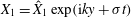 $X_{1}=\hat{X}_{1}\exp (\text{i}ky+\unicode[STIX]{x1D70E}t)$
and
$X_{1}=\hat{X}_{1}\exp (\text{i}ky+\unicode[STIX]{x1D70E}t)$
and
 $X=(H(x,y,t),\boldsymbol{u}(x,y,z,t),\boldsymbol{q}(x,y,t))$
. With the assumption that the perturbations to the flow are resisted dominantly by horizontal shear stresses, the gradients in
$X=(H(x,y,t),\boldsymbol{u}(x,y,z,t),\boldsymbol{q}(x,y,t))$
. With the assumption that the perturbations to the flow are resisted dominantly by horizontal shear stresses, the gradients in
 $z$
are negligible and so the perturbation to the velocity obeys
$z$
are negligible and so the perturbation to the velocity obeys
 $$\begin{eqnarray}\boldsymbol{u}_{\mathbf{1}}=-\frac{1}{k^{2}}\unicode[STIX]{x1D735}H_{1}.\end{eqnarray}$$
In contrast with the previous analysis, here the velocity involves a
 $1/k^{2}$
contribution, reflecting the resistence to the flow by horizontal shear stresses. We will use the convention that the
$1/k^{2}$
contribution, reflecting the resistence to the flow by horizontal shear stresses. We will use the convention that the
 $y$
-component of the gradient operator means either
$y$
-component of the gradient operator means either
 $\text{d}/\text{d}y$
or
$\text{d}/\text{d}y$
or
 $\text{i}k$
, interchangeably.
$\text{i}k$
, interchangeably.
The volume flux, per unit width, can be expressed as
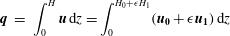 $$\begin{eqnarray}\displaystyle \boldsymbol{q} & = & \displaystyle \int _{0}^{H}\boldsymbol{u}\,\text{d}z=\int _{0}^{H_{0}+\unicode[STIX]{x1D716}H_{1}}(\boldsymbol{u}_{\mathbf{0}}+\unicode[STIX]{x1D716}\boldsymbol{u}_{\mathbf{1}})\,\text{d}z\end{eqnarray}$$
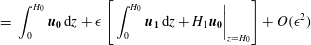 $$\begin{eqnarray}\displaystyle & = & \displaystyle \int _{0}^{H_{0}}\boldsymbol{u}_{\mathbf{0}}\,\text{d}z+\unicode[STIX]{x1D716}\left[\left.\int _{0}^{H_{0}}\boldsymbol{u}_{\mathbf{1}}\,\text{d}z+H_{1}\boldsymbol{u}_{\mathbf{0}}\right|_{z=H_{0}}\right]+O(\unicode[STIX]{x1D716}^{2})\end{eqnarray}$$
so that the perturbation to the volume flux, per unit width, is
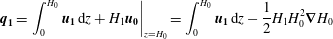 $$\begin{eqnarray}\boldsymbol{q}_{\mathbf{1}}=\left.\int _{0}^{H_{0}}\boldsymbol{u}_{\mathbf{1}}\,\text{d}z+H_{1}\boldsymbol{u}_{\mathbf{0}}\right|_{z=H_{0}}=\int _{0}^{H_{0}}\boldsymbol{u}_{\mathbf{1}}\,\text{d}z-\frac{1}{2}H_{1}H_{0}^{2}\unicode[STIX]{x1D735}H_{0}\end{eqnarray}$$
since the basic-state velocity for a classical current is primarily along the
 $x$
-direction with
$x$
-direction with
 $u_{0}=-(1/2)z(2H_{0}-z)\unicode[STIX]{x2202}H_{0}/\unicode[STIX]{x2202}x$
. Substituting the expression (5.1) for the perturbation to the velocity gives
$u_{0}=-(1/2)z(2H_{0}-z)\unicode[STIX]{x2202}H_{0}/\unicode[STIX]{x2202}x$
. Substituting the expression (5.1) for the perturbation to the velocity gives
 $$\begin{eqnarray}\boldsymbol{q}_{\mathbf{1}}=-\frac{1}{k^{2}}H_{0}\unicode[STIX]{x1D735}H_{1}-\frac{1}{2}H_{1}H_{0}^{2}\unicode[STIX]{x1D735}H_{0}.\end{eqnarray}$$
This differs from (4.8) in the
 $1/k^{2}$
term to reflect that the flow of the perturbations is resisted by horizontal shear. The time evolution of the perturbations, in the frame of the lubrication front, is governed by the mass conservation equation for the next order in
$1/k^{2}$
term to reflect that the flow of the perturbations is resisted by horizontal shear. The time evolution of the perturbations, in the frame of the lubrication front, is governed by the mass conservation equation for the next order in
 $\unicode[STIX]{x1D716}$
:
$\unicode[STIX]{x1D716}$
:
 $$\begin{eqnarray}\displaystyle \unicode[STIX]{x1D70E}H_{1}-V\frac{\unicode[STIX]{x2202}H_{1}}{\unicode[STIX]{x2202}x} & = & \displaystyle -\unicode[STIX]{x1D735}\boldsymbol{\cdot }\boldsymbol{q}_{\pmb{{\it 1}}}\nonumber\\ \displaystyle & = & \displaystyle -\frac{\unicode[STIX]{x2202}}{\unicode[STIX]{x2202}x}(\boldsymbol{q}_{\mathbf{1}}\boldsymbol{\cdot }\boldsymbol{e}_{\boldsymbol{x}})-\text{i}k\boldsymbol{q}_{\mathbf{1}}\boldsymbol{\cdot }\boldsymbol{e}_{\boldsymbol{y}}.\end{eqnarray}$$
5.1.2 Lubricated region
We introduce small perturbations of size
 $\unicode[STIX]{x1D716}\ll 1$
and investigate the stability of the flow by searching for normal-mode solutions with transverse wavenumber
$\unicode[STIX]{x1D716}\ll 1$
and investigate the stability of the flow by searching for normal-mode solutions with transverse wavenumber
 $k$
and growth rate
$k$
and growth rate
 $\unicode[STIX]{x1D70E}$
. We expand in series of
$\unicode[STIX]{x1D70E}$
. We expand in series of
 $\unicode[STIX]{x1D716}$
,
$\unicode[STIX]{x1D716}$
,
 $Y=Y_{0}+\unicode[STIX]{x1D716}Y_{1}$
where
$Y=Y_{0}+\unicode[STIX]{x1D716}Y_{1}$
where
 $Y_{1}={\hat{Y}}_{1}\exp (\text{i}ky+\unicode[STIX]{x1D70E}t),$
and
$Y_{1}={\hat{Y}}_{1}\exp (\text{i}ky+\unicode[STIX]{x1D70E}t),$
and
 $$\begin{eqnarray}Y=[H(x,y,t),h(x,y,t),\boldsymbol{u}(x,y,z,t),\boldsymbol{u}_{\boldsymbol{l}}(x,y,z,t),\boldsymbol{q}(x,y,t),\boldsymbol{q}_{\boldsymbol{l}}(x,y,t)].\end{eqnarray}$$
As the perturbations to the flow are resisted dominantly by horizontal shear stresses, the gradients in
 $z$
are negligible and so
$z$
are negligible and so
 $$\begin{eqnarray}\boldsymbol{u}_{\mathbf{1}}=-\frac{1}{k^{2}}\unicode[STIX]{x1D735}H_{1}\end{eqnarray}$$
for the upper layer and
 $$\begin{eqnarray}\boldsymbol{u}_{\boldsymbol{l}\mathbf{1}}=-\frac{{\mathcal{M}}}{k^{2}}\unicode[STIX]{x1D735}H_{1}\end{eqnarray}$$
for the lower layer. There is a small boundary layer at the interface between the two fluids and at the base, in which vertical shear stresses are important and resolve the no-slip boundary condition as well as the continuity of velocity and shear stress at the interface. However, the effect of this boundary layer is negligible in a depth-averaged description of the flow when the wavenumber of the perturbations is large, specifically when
 $k\gg 1/h$
. As an alternative to scaling arguments, this can also be deduced from considering the full calculation with
$k\gg 1/h$
. As an alternative to scaling arguments, this can also be deduced from considering the full calculation with
 $k=O(1)$
so that both vertical and transverse shear contribute to resisting the perturbations to the flow, and considering the limit
$k=O(1)$
so that both vertical and transverse shear contribute to resisting the perturbations to the flow, and considering the limit
 $kh\rightarrow \infty$
.
$kh\rightarrow \infty$
.
The volume flux, per unit width, of the upper layer fluid is
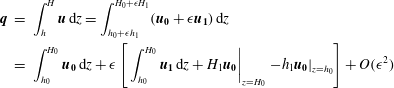 $$\begin{eqnarray}\displaystyle \boldsymbol{q} & = & \displaystyle \int _{h}^{H}\boldsymbol{u}\,\text{d}z=\int _{h_{0}+\unicode[STIX]{x1D716}h_{1}}^{H_{0}+\unicode[STIX]{x1D716}H_{1}}(\boldsymbol{u}_{\mathbf{0}}+\unicode[STIX]{x1D716}\boldsymbol{u}_{\mathbf{1}})\,\text{d}z\nonumber\\ \displaystyle & = & \displaystyle \int _{h_{0}}^{H_{0}}\boldsymbol{u}_{\mathbf{0}}\,\text{d}z+\unicode[STIX]{x1D716}\left[\left.\int _{h_{0}}^{H_{0}}\boldsymbol{u}_{\boldsymbol{ 1}}\,\text{d}z+H_{1}\boldsymbol{u}_{\mathbf{0}}\right|_{z=H_{0}}\left.-h_{1}\boldsymbol{u}_{\mathbf{0}}\right|_{z=h_{0}}\right]+O(\unicode[STIX]{x1D716}^{2})\end{eqnarray}$$
and in the lower layer is
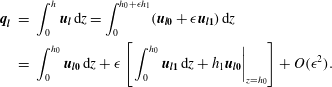 $$\begin{eqnarray}\displaystyle \boldsymbol{q}_{\boldsymbol{l}} & = & \displaystyle \int _{0}^{h}\boldsymbol{u}_{\boldsymbol{l}}\,\text{d}z=\int _{0}^{h_{0}+\unicode[STIX]{x1D716}h_{1}}(\boldsymbol{u}_{\boldsymbol{l}\mathbf{0}}+\unicode[STIX]{x1D716}\boldsymbol{u}_{\boldsymbol{l}\mathbf{1}})\,\text{d}z\nonumber\\ \displaystyle & = & \displaystyle \int _{0}^{h_{0}}\boldsymbol{u}_{\boldsymbol{l}\mathbf{0}}\,\text{d}z+\unicode[STIX]{x1D716}\left[\left.\int _{0}^{h_{0}}\boldsymbol{u}_{\boldsymbol{l}\mathbf{1}}\,\text{d}z+h_{1}\boldsymbol{u}_{\boldsymbol{l}\mathbf{0}}\right|_{z=h_{0}}\right]+O(\unicode[STIX]{x1D716}^{2}).\end{eqnarray}$$
By using expressions for the velocity fields for the two layers at zeroth order in
 $\unicode[STIX]{x1D716}$
given Kowal & Worster (Reference Kowal and Worster2015), the perturbation to the volume flux in the upper layer can be found to be
$\unicode[STIX]{x1D716}$
given Kowal & Worster (Reference Kowal and Worster2015), the perturbation to the volume flux in the upper layer can be found to be
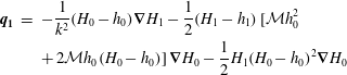 $$\begin{eqnarray}\displaystyle \boldsymbol{q}_{\mathbf{1}} & = & \displaystyle -\frac{1}{k^{2}}(H_{0}-h_{0})\unicode[STIX]{x1D735}H_{1}-\frac{1}{2}(H_{1}-h_{1})[\!{\mathcal{M}}h_{0}^{2}\nonumber\\ \displaystyle & & \displaystyle +\,2{\mathcal{M}}h_{0}(H_{0}-h_{0})\!]\unicode[STIX]{x1D735}H_{0}-\frac{1}{2}H_{1}(H_{0}-h_{0})^{2}\unicode[STIX]{x1D735}H_{0}\end{eqnarray}$$
and in the lower layer to be
 $$\begin{eqnarray}\boldsymbol{q}_{\boldsymbol{l}\mathbf{1}}=-\frac{1}{k^{2}}{\mathcal{M}}H_{0}\unicode[STIX]{x1D735}H_{1}-\frac{1}{2}h_{1}[{\mathcal{M}}h_{0}^{2}+2{\mathcal{M}}h_{0}(H_{0}-h_{0})]\unicode[STIX]{x1D735}H_{0}.\end{eqnarray}$$
These differ from (4.6) and (4.7) in the
 $1/k^{2}$
term, as before. Conservation of mass at first order in
$1/k^{2}$
term, as before. Conservation of mass at first order in
 $\unicode[STIX]{x1D716}$
in the two layers is described by
$\unicode[STIX]{x1D716}$
in the two layers is described by
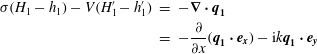 $$\begin{eqnarray}\displaystyle \unicode[STIX]{x1D70E}(H_{1}-h_{1})-V(H_{1}^{\prime }-h_{1}^{\prime }) & = & \displaystyle -\unicode[STIX]{x1D735}\boldsymbol{\cdot }\boldsymbol{q}_{\mathbf{1}}\nonumber\\ \displaystyle & = & \displaystyle -\frac{\unicode[STIX]{x2202}}{\unicode[STIX]{x2202}x}(\boldsymbol{q}_{\mathbf{1}}\boldsymbol{\cdot }\boldsymbol{e}_{\boldsymbol{x}})-\text{i}k\boldsymbol{q}_{\mathbf{1}}\boldsymbol{\cdot }\boldsymbol{e}_{\boldsymbol{y}}\end{eqnarray}$$
for the upper layer and
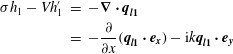 $$\begin{eqnarray}\displaystyle \unicode[STIX]{x1D70E}h_{1}-Vh_{1}^{\prime } & = & \displaystyle -\unicode[STIX]{x1D735}\boldsymbol{\cdot }\boldsymbol{q}_{\boldsymbol{l}\mathbf{1}}\nonumber\\ \displaystyle & = & \displaystyle -\frac{\unicode[STIX]{x2202}}{\unicode[STIX]{x2202}x}(\boldsymbol{q}_{\boldsymbol{l}\mathbf{1}}\boldsymbol{\cdot }\boldsymbol{e}_{\boldsymbol{x}})-\text{i}k\boldsymbol{q}_{\boldsymbol{l}\mathbf{1}}\boldsymbol{\cdot }\boldsymbol{e}_{\boldsymbol{y}}\end{eqnarray}$$
for the lower layer. Here, we take the basic state to be quasi-steady with respect to the lubrication front.
5.2 Local stability analysis: results
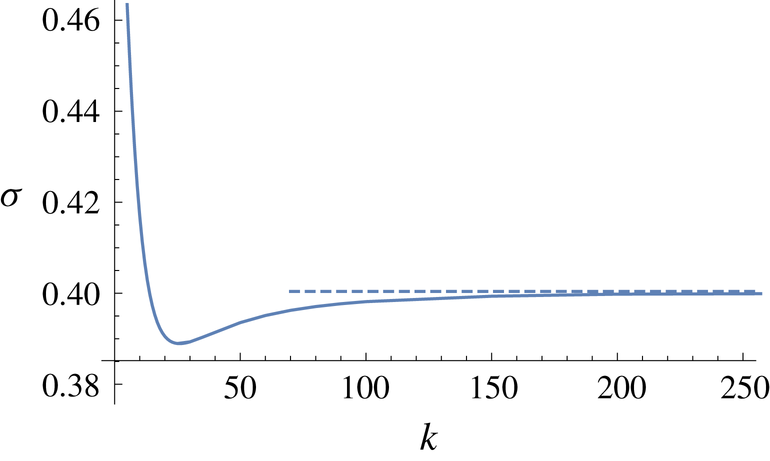
Figure 6. Asymptotic (dashed) and numerical (solid) solutions for the growth rates
 $\unicode[STIX]{x1D70E}$
against wavenumber
$\unicode[STIX]{x1D70E}$
against wavenumber
 $k$
for perturbations resisted dominantly by horizontal shear. Parameter values used are
$k$
for perturbations resisted dominantly by horizontal shear. Parameter values used are
 ${\mathcal{M}}=10$
and
${\mathcal{M}}=10$
and
 ${\mathcal{Q}}=0.1$
.
${\mathcal{Q}}=0.1$
.
We locally approximate the basic-state surface heights linearly near the lubrication front and summarise the resulting set of equations in the lubricated and unlubricated regions along with jump conditions in (E 1)–(E 9) of appendix E. The method used to derive these local equations, valid in the vicinity of the lubrication front, follows that of the previous section on perturbations resisted dominantly by vertical shear. We solve these equations explicitly to obtain the dispersion relation in § E.0.2 and also perform an asymptotic analysis for large wavenumbers
 $k$
. The asymptotics are outlined in § E.0.3 of appendix E. The main message to take away can be captured concisely in the limit of
$k$
. The asymptotics are outlined in § E.0.3 of appendix E. The main message to take away can be captured concisely in the limit of
 ${\mathcal{M}}\rightarrow \infty$
, in which the large-
${\mathcal{M}}\rightarrow \infty$
, in which the large-
 $k$
behaviour of
$k$
behaviour of
 $\unicode[STIX]{x1D70E}$
is given by the simple relation
$\unicode[STIX]{x1D70E}$
is given by the simple relation
 $$\begin{eqnarray}\unicode[STIX]{x1D70E}=\frac{\unicode[STIX]{x1D711}_{8}{\mathcal{M}}^{2}+\unicode[STIX]{x1D711}_{9}{\mathcal{M}}}{\unicode[STIX]{x1D711}_{10}}+O(1/k,1/{\mathcal{M}}),\end{eqnarray}$$
where
 $\unicode[STIX]{x1D711}_{8},\ldots ,\unicode[STIX]{x1D711}_{10}$
are functions of the basic state thicknesses, slopes and lubrication front velocity. Explicit expressions can be found in (S.113)–(S.115) of the supplementary material. The important message is that
$\unicode[STIX]{x1D711}_{8},\ldots ,\unicode[STIX]{x1D711}_{10}$
are functions of the basic state thicknesses, slopes and lubrication front velocity. Explicit expressions can be found in (S.113)–(S.115) of the supplementary material. The important message is that
 $\unicode[STIX]{x1D70E}$
tends to a constant at large wavenumbers. This, in fact, is the case not only in the limit
$\unicode[STIX]{x1D70E}$
tends to a constant at large wavenumbers. This, in fact, is the case not only in the limit
 ${\mathcal{M}}\rightarrow \infty$
, but holds for any value of
${\mathcal{M}}\rightarrow \infty$
, but holds for any value of
 ${\mathcal{M}}$
and indicates that horizontal shear significantly stabilises the flow at large wavenumber.
${\mathcal{M}}$
and indicates that horizontal shear significantly stabilises the flow at large wavenumber.
The large-
 $k$
asymptotic solution for the growth rate
$k$
asymptotic solution for the growth rate
 $\unicode[STIX]{x1D70E}$
is shown in figure 6, where it is additionally seen that the full numerical solution of the equations (E 1)–(E 9) described in appendix E for the growth rate converges towards the asymptotic result.
$\unicode[STIX]{x1D70E}$
is shown in figure 6, where it is additionally seen that the full numerical solution of the equations (E 1)–(E 9) described in appendix E for the growth rate converges towards the asymptotic result.
This analysis reveals that horizontal shear provides a desirable stabilising mechanism for large wavenumbers. In the following section, we combine the physical ideas of § 4 and the current section to determine the behaviour at intermediate wavenumbers.
6 Frontal dynamics: intermediate regime for perturbations resisted by vertical and horizontal shear
In this section, we consider the intermediate regime in which the flow of the basic state is resisted dominantly by vertical shear stresses while the flow of the perturbations is resisted dominantly by both vertical and horizontal shear stresses.
6.1 Model equations
6.1.1 Unlubricated region
With the lubrication approximation, the Stokes equations for the fluid flow in the unlubricated region are given by
 $$\begin{eqnarray}0=-\unicode[STIX]{x1D735}p-\boldsymbol{e}_{\boldsymbol{z}}+\left(\frac{\unicode[STIX]{x2202}^{2}}{\unicode[STIX]{x2202}y^{2}}+\frac{\unicode[STIX]{x2202}^{2}}{\unicode[STIX]{x2202}z^{2}}\right)\boldsymbol{u}\end{eqnarray}$$
in dimensionless variables. A vertical balance of forces gives that the pressure is given hydrostatically by
 $$\begin{eqnarray}p=H-z,\end{eqnarray}$$
whereas a horizontal balance gives
 $$\begin{eqnarray}\unicode[STIX]{x1D735}H=\left(\frac{\unicode[STIX]{x2202}^{2}}{\unicode[STIX]{x2202}y^{2}}+\frac{\unicode[STIX]{x2202}^{2}}{\unicode[STIX]{x2202}z^{2}}\right)\boldsymbol{u}.\end{eqnarray}$$
To investigate the stability of the flow, we introduce small disturbances of size
 $\unicode[STIX]{x1D716}\ll 1$
and search for normal-mode solutions with transverse wavenumber
$\unicode[STIX]{x1D716}\ll 1$
and search for normal-mode solutions with transverse wavenumber
 $k$
and growth rate
$k$
and growth rate
 $\unicode[STIX]{x1D70E}$
of the form
$\unicode[STIX]{x1D70E}$
of the form
 $X=X_{0}+\unicode[STIX]{x1D716}X_{1}+\cdots \,$
, where
$X=X_{0}+\unicode[STIX]{x1D716}X_{1}+\cdots \,$
, where
 $X_{1}=\hat{X}_{1}\exp (\text{i}ky+\unicode[STIX]{x1D70E}t)$
and
$X_{1}=\hat{X}_{1}\exp (\text{i}ky+\unicode[STIX]{x1D70E}t)$
and
 $X=(H(x,y,t),\boldsymbol{u}(x,y,z,t),\boldsymbol{q}(x,y,t))$
. The horizontal part of Stokes equations becomes
$X=(H(x,y,t),\boldsymbol{u}(x,y,z,t),\boldsymbol{q}(x,y,t))$
. The horizontal part of Stokes equations becomes
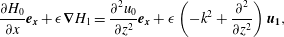 $$\begin{eqnarray}\frac{\unicode[STIX]{x2202}H_{0}}{\unicode[STIX]{x2202}x}\boldsymbol{e}_{\boldsymbol{x}}+\unicode[STIX]{x1D716}\unicode[STIX]{x1D735}H_{1}=\frac{\unicode[STIX]{x2202}^{2}u_{0}}{\unicode[STIX]{x2202}z^{2}}\boldsymbol{e}_{\boldsymbol{x}}+\unicode[STIX]{x1D716}\left(-k^{2}+\frac{\unicode[STIX]{x2202}^{2}}{\unicode[STIX]{x2202}z^{2}}\right)\boldsymbol{u}_{\mathbf{1}},\end{eqnarray}$$
which has the following contribution at
 $O(\unicode[STIX]{x1D716})$
:
$O(\unicode[STIX]{x1D716})$
:
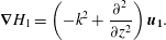 $$\begin{eqnarray}\unicode[STIX]{x1D735}H_{1}=\left(-k^{2}+\frac{\unicode[STIX]{x2202}^{2}}{\unicode[STIX]{x2202}z^{2}}\right)\boldsymbol{u}_{\mathbf{1}}.\end{eqnarray}$$
For intermediate wavenumbers
 $k$
, the effect of both horizontal and vertical shear stresses can become important and we retain both in the governing equations. The perturbed velocity is therefore exponential in
$k$
, the effect of both horizontal and vertical shear stresses can become important and we retain both in the governing equations. The perturbed velocity is therefore exponential in
 $z$
and resolves the boundary layers that were previously neglected in the limit in which horizontal shear was dominant. The full details are given in (F 1)–(F 2) of appendix F, where the perturbed velocities and fluxes are given explicitly along with the mass conservation equations. We further apply local approximations valid in the vicinity of the lubrication front and match to the outer regions through decay conditions. This enables us to search for normal-mode solutions. The approach follows that of the previous two sections.
$z$
and resolves the boundary layers that were previously neglected in the limit in which horizontal shear was dominant. The full details are given in (F 1)–(F 2) of appendix F, where the perturbed velocities and fluxes are given explicitly along with the mass conservation equations. We further apply local approximations valid in the vicinity of the lubrication front and match to the outer regions through decay conditions. This enables us to search for normal-mode solutions. The approach follows that of the previous two sections.
6.2 Lubricated region
Linearising the Stokes equations and looking for normal-mode solutions, while keeping the terms arising from both vertical and horizontal shear stresses, gives the following horizontal part of Stokes equations:
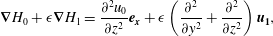 $$\begin{eqnarray}\displaystyle & \displaystyle \unicode[STIX]{x1D735}H_{0}+\unicode[STIX]{x1D716}\unicode[STIX]{x1D735}H_{1}=\frac{\unicode[STIX]{x2202}^{2}u_{0}}{\unicode[STIX]{x2202}z^{2}}\boldsymbol{e}_{\boldsymbol{x}}+\unicode[STIX]{x1D716}\left(\frac{\unicode[STIX]{x2202}^{2}}{\unicode[STIX]{x2202}y^{2}}+\frac{\unicode[STIX]{x2202}^{2}}{\unicode[STIX]{x2202}z^{2}}\right)\boldsymbol{u}_{\mathbf{1}}, & \displaystyle\end{eqnarray}$$
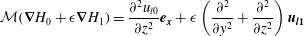 $$\begin{eqnarray}\displaystyle & \displaystyle {\mathcal{M}}(\unicode[STIX]{x1D735}H_{0}+\unicode[STIX]{x1D716}\unicode[STIX]{x1D735}H_{1})=\frac{\unicode[STIX]{x2202}^{2}u_{l0}}{\unicode[STIX]{x2202}z^{2}}\boldsymbol{e}_{\boldsymbol{x}}+\unicode[STIX]{x1D716}\left(\frac{\unicode[STIX]{x2202}^{2}}{\unicode[STIX]{x2202}y^{2}}+\frac{\unicode[STIX]{x2202}^{2}}{\unicode[STIX]{x2202}z^{2}}\right)\boldsymbol{u}_{\boldsymbol{l}\mathbf{1}} & \displaystyle\end{eqnarray}$$
for the two layers. This yields the following
 $O(\unicode[STIX]{x1D716})$
contributions:
$O(\unicode[STIX]{x1D716})$
contributions:
 $$\begin{eqnarray}\displaystyle & \displaystyle \unicode[STIX]{x1D735}H_{1}=\left(\frac{\unicode[STIX]{x2202}^{2}}{\unicode[STIX]{x2202}y^{2}}+\frac{\unicode[STIX]{x2202}^{2}}{\unicode[STIX]{x2202}z^{2}}\right)\boldsymbol{u}_{\mathbf{1}}, & \displaystyle\end{eqnarray}$$
 $$\begin{eqnarray}\displaystyle & \displaystyle {\mathcal{M}}\unicode[STIX]{x1D735}H_{1}=\left(\frac{\unicode[STIX]{x2202}^{2}}{\unicode[STIX]{x2202}y^{2}}+\frac{\unicode[STIX]{x2202}^{2}}{\unicode[STIX]{x2202}z^{2}}\right)\boldsymbol{u}_{\boldsymbol{l}\mathbf{1}} & \displaystyle\end{eqnarray}$$
for the two layers. As the perturbations to the flow are resisted by both vertical and horizontal shear stresses, the gradients in
 $z$
are comparable to the gradients in
$z$
are comparable to the gradients in
 $y$
. We therefore retain both and by looking for normal-mode solutions obtain the following equations for the horizontal velocity:
$y$
. We therefore retain both and by looking for normal-mode solutions obtain the following equations for the horizontal velocity:
 $$\begin{eqnarray}\unicode[STIX]{x1D735}H_{1}=\left(-k^{2}+\frac{\unicode[STIX]{x2202}^{2}}{\unicode[STIX]{x2202}z^{2}}\right)\boldsymbol{u}_{\mathbf{1}}\end{eqnarray}$$
for the upper layer and
 $$\begin{eqnarray}\unicode[STIX]{x1D735}H_{1}=\left(-k^{2}+\frac{\unicode[STIX]{x2202}^{2}}{\unicode[STIX]{x2202}z^{2}}\right)\boldsymbol{u}_{\boldsymbol{l}\mathbf{1}}\end{eqnarray}$$
for the lower layer. This approach resolves the small boundary layer at the interface between the two fluids and at the base, in which vertical shear stresses are important. The limit
 $kh\rightarrow \infty$
simplifies the problem to that of the previous section, in which horizontal shear stresses provide the dominant resistance to the flow of the perturbations and in which the effect of this boundary layer is negligible in a depth-averaged description of the flow.
$kh\rightarrow \infty$
simplifies the problem to that of the previous section, in which horizontal shear stresses provide the dominant resistance to the flow of the perturbations and in which the effect of this boundary layer is negligible in a depth-averaged description of the flow.
6.3 Local stability analysis: results
Due to the terms proportional to
 $-k^{2}$
, the horizontal velocities are given in terms of exponentials in
$-k^{2}$
, the horizontal velocities are given in terms of exponentials in
 $z$
(in a finite domain) and present difficulties in obtaining a concise lubrication model. The reader is referred to appendix F, specifically (F 1)–(F 2) and (F 7)–(F 10), where the details of the derivation of the model as well as the application of the local approximation and matching to the outer regions can be found.
$z$
(in a finite domain) and present difficulties in obtaining a concise lubrication model. The reader is referred to appendix F, specifically (F 1)–(F 2) and (F 7)–(F 10), where the details of the derivation of the model as well as the application of the local approximation and matching to the outer regions can be found.
Figure 7 shows the growth rates
 $\unicode[STIX]{x1D70E}$
as a function of the transverse wavenumber
$\unicode[STIX]{x1D70E}$
as a function of the transverse wavenumber
 $k$
for representative parameter values, for the intermediate regime, considered in this section, in which the perturbations are resisted by both vertical and horizontal shear. Figure 7 also displays the growth rates for the small-wavenumber limit in which vertical shear provides the dominant resistance to the flow of the perturbations and also the large-wavenumber limit in which horizontal shear provides the dominant resistance to the flow of the perturbations. The intermediate regime, involving both vertical and horizontal shear stresses, is seen to converge to these small- and large-wavenumber limits in figure 7.
$k$
for representative parameter values, for the intermediate regime, considered in this section, in which the perturbations are resisted by both vertical and horizontal shear. Figure 7 also displays the growth rates for the small-wavenumber limit in which vertical shear provides the dominant resistance to the flow of the perturbations and also the large-wavenumber limit in which horizontal shear provides the dominant resistance to the flow of the perturbations. The intermediate regime, involving both vertical and horizontal shear stresses, is seen to converge to these small- and large-wavenumber limits in figure 7.

Figure 7. Growth rates
 $\unicode[STIX]{x1D70E}$
against wavenumber
$\unicode[STIX]{x1D70E}$
against wavenumber
 $k$
for perturbations resisted by vertical shear only (dotted), horizontal shear only (dashed) and both vertical and horizontal shear (solid). This figure uses results presented in figure 6 (dashed) for
$k$
for perturbations resisted by vertical shear only (dotted), horizontal shear only (dashed) and both vertical and horizontal shear (solid). This figure uses results presented in figure 6 (dashed) for
 $k\gg 1$
. Parameter values used are
$k\gg 1$
. Parameter values used are
 ${\mathcal{M}}=10$
and
${\mathcal{M}}=10$
and
 ${\mathcal{Q}}=0.1$
.
${\mathcal{Q}}=0.1$
.
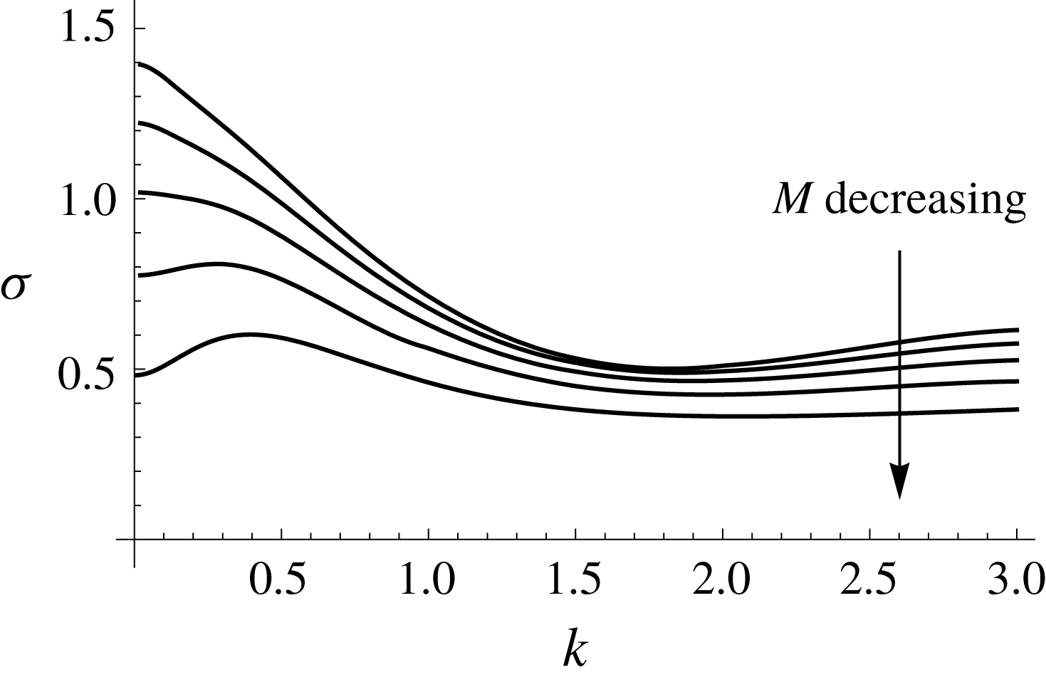
Figure 8. Growth rates
 $\unicode[STIX]{x1D70E}$
against wavenumber
$\unicode[STIX]{x1D70E}$
against wavenumber
 $k$
for perturbations resisted by both vertical and horizontal shear. Parameter values used are
$k$
for perturbations resisted by both vertical and horizontal shear. Parameter values used are
 ${\mathcal{M}}=10$
, 15, 20, 25, 30 and
${\mathcal{M}}=10$
, 15, 20, 25, 30 and
 ${\mathcal{Q}}=0.1$
.
${\mathcal{Q}}=0.1$
.
Apart from the large-wavenumber stabilisation analysed in the previous section, horizontal shear also stabilises the flow at small wavenumbers. Figure 8 shows representative growth rates as a function of the wavenumber, for the intermediate regime, involving both vertical and horizontal shear stresses, for varying viscosity ratios
 ${\mathcal{M}}$
. It is seen that small wavenumbers are the most unstable, and that the band of most unstable wavenumbers shifts towards smaller wavenumbers as the viscosity ratio increases. This does not necessarily imply that
${\mathcal{M}}$
. It is seen that small wavenumbers are the most unstable, and that the band of most unstable wavenumbers shifts towards smaller wavenumbers as the viscosity ratio increases. This does not necessarily imply that
 $k=0$
is the most unstable wavenumber for these viscosity ratios, as a non-local analysis, valid for small wavenumbers, would be necessary to examine this.
$k=0$
is the most unstable wavenumber for these viscosity ratios, as a non-local analysis, valid for small wavenumbers, would be necessary to examine this.
7 Conclusions
We have carried out linear stability analyses of lubricated viscous gravity currents in two scenarios to isolate two different mechanisms of instability: internal and frontal. The former analysis shows that steady flow with no internal front is unconditionally stable and suggests that the instability observed in experiments is a frontal instability. The latter analysis explains the mechanism of instability by exploring three physical scenarios.
The first scenario occurs for wavelengths much larger than the thicknesses of the two layers. We highlighted the underlying physical mechanism that drives the instability by using a combination of asymptotic and numerical methods. Analytically, we derived an asymptotic solution for the growth rate of the perturbations as an outer, large-wavenumber limit, which shows that the growth rate
 $\unicode[STIX]{x1D70E}$
of the perturbations grows linearly with the wavenumber
$\unicode[STIX]{x1D70E}$
of the perturbations grows linearly with the wavenumber
 $k$
as
$k$
as
 $k\rightarrow \infty$
with a prefactor that depends on the two layer thicknesses, the viscosity ratio as well as, crucially, the jump in upper surface slope, or hydrostatic pressure gradient, across the lubrication front. The latter ingredient, importantly, determines the sign of
$k\rightarrow \infty$
with a prefactor that depends on the two layer thicknesses, the viscosity ratio as well as, crucially, the jump in upper surface slope, or hydrostatic pressure gradient, across the lubrication front. The latter ingredient, importantly, determines the sign of
 $\unicode[STIX]{x1D70E}$
, that is, it determines whether or not the flow is unstable. By balancing upstream and downstream upper-layer fluxes, we further showed that this jump in upper-surface slope is positive (that is, the flow is stable) precisely when the viscosity ratio
$\unicode[STIX]{x1D70E}$
, that is, it determines whether or not the flow is unstable. By balancing upstream and downstream upper-layer fluxes, we further showed that this jump in upper-surface slope is positive (that is, the flow is stable) precisely when the viscosity ratio
 ${\mathcal{M}}$
between the two layers is less than one. That is, when a less viscous fluid lubricates a more viscous fluid – the setting relevant to our experiments and of geophysical interest – then the lubrication front is unstable; whereas if the situation is reversed and a more viscous fluid is injected underneath a less viscous fluid, then the flow remains stable.
${\mathcal{M}}$
between the two layers is less than one. That is, when a less viscous fluid lubricates a more viscous fluid – the setting relevant to our experiments and of geophysical interest – then the lubrication front is unstable; whereas if the situation is reversed and a more viscous fluid is injected underneath a less viscous fluid, then the flow remains stable.
The underlying instability mechanism involves a jump in hydrostatic pressure gradient across the lubrication front in contrast to Saffman–Taylor fingering, which occurs as a result of a jump in dynamic pressure gradient across the intrusion front. The instability mechanism can be understood physically by considering the lubrication front in the case in which a less viscous fluid intrudes beneath a more viscous fluid. If the lubrication front is perturbed so that the underlying, less viscous fluid dislocates to the no-slip region, then it becomes subject to higher hydrostatic pressure gradients and advances forward, feeding the instability. In the opposite case in which a more viscous fluid intrudes underneath a less viscous fluid, then if the front is perturbed so that the underlying more viscous fluid dislocates to the no-slip region, then it becomes subject to lower hydrostatic pressure gradients and slows down, suppressing the instability.
By using a combination of asymptotic and numerical methods, we found that for the second scenario, involving perturbations resisted dominantly by horizontal shear stresses, the growth rate of the perturbations converges towards a constant rather than growing unboundedly. Transverse shear, therefore, provides an effective but weak stabilising mechanism at large wavenumbers. By considering the third, intermediate regime and formulating a fuller theoretical model accounting for both vertical and transverse shear stresses and solving it numerically, we found that transverse shear is weakly stabilising for intermediate wavenumbers as well and that intermediate wavenumbers are the most unstable at modest values of
 ${\mathcal{M}}$
. For larger values of
${\mathcal{M}}$
. For larger values of
 ${\mathcal{M}}$
, long waves are selected. In the companion paper, we consider effects of buoyancy and find further stabilisation at long wavelengths.
${\mathcal{M}}$
, long waves are selected. In the companion paper, we consider effects of buoyancy and find further stabilisation at long wavelengths.
Acknowledgement
K.N.K. acknowledges the support of a NERC PhD studentship.
Supplementary material
Full expressions for coefficients used within this paper can be found in the supplementary material available at https://doi.org/10.1017/jfm.2019.321.
Appendix A. Tensorial form for lubricated currents with drainage
The prefactors
 $a$
and
$a$
and
 $A$
depend on the dimensionless parameters via
$A$
depend on the dimensionless parameters via
 $$\begin{eqnarray}\displaystyle & \displaystyle \frac{1}{4}\left[\frac{{\mathcal{M}}}{3}a^{3}({\mathcal{D}}a+A)+\frac{{\mathcal{M}}}{2}a^{2}A(A-a)\right]={\mathcal{Q}}, & \displaystyle\end{eqnarray}$$
 $$\begin{eqnarray}\displaystyle & \displaystyle \frac{1}{4}\left[\frac{1}{3}(A-a)^{3}A+\frac{{\mathcal{M}}}{2}a^{2}(A-a)({\mathcal{D}}a+A)+{\mathcal{M}}aA(A-a)^{2}\right]=1. & \displaystyle\end{eqnarray}$$
The entries of
 $\unicode[STIX]{x1D63E}$
are given by
$\unicode[STIX]{x1D63E}$
are given by
 $$\begin{eqnarray}\unicode[STIX]{x1D60A}_{11}=1,\quad \unicode[STIX]{x1D60A}_{12}=0,\quad \unicode[STIX]{x1D60A}_{21}=-1,\quad \unicode[STIX]{x1D60A}_{22}=1,\end{eqnarray}$$
the entries of
 $\unicode[STIX]{x1D640}$
are given by
$\unicode[STIX]{x1D640}$
are given by
 $$\begin{eqnarray}\left.\begin{array}{@{}c@{}}\unicode[STIX]{x1D60C}_{11}={\displaystyle \frac{{\mathcal{M}}D}{3}}a^{3},\\ \unicode[STIX]{x1D60C}_{12}={\displaystyle \frac{{\mathcal{M}}}{3}}a^{3}+{\displaystyle \frac{{\mathcal{M}}}{2}}a^{2}(A-a),\\ \unicode[STIX]{x1D60C}_{21}={\displaystyle \frac{{\mathcal{M}}D}{2}}a^{2}(A-a),\\ \unicode[STIX]{x1D60C}_{22}={\displaystyle \frac{1}{3}}(A-a)^{3}+{\displaystyle \frac{{\mathcal{M}}}{2}}a^{2}(A-a)+{\mathcal{M}}a(A-a)^{2}\end{array}\right\}\end{eqnarray}$$
and the entries of
 $\unicode[STIX]{x1D641}$
are given by
$\unicode[STIX]{x1D641}$
are given by
 $$\begin{eqnarray}\left.\begin{array}{@{}c@{}}\unicode[STIX]{x1D60D}_{11}={\mathcal{M}}a^{2}({\mathcal{D}}a+A)+{\displaystyle \frac{{\mathcal{M}}}{2}}(-a^{2}A+2aA(A-a)),\\ \unicode[STIX]{x1D60D}_{12}={\displaystyle \frac{{\mathcal{M}}}{2}}a^{2}A,\\ \unicode[STIX]{x1D60D}_{21}=-(A-a)^{2}A+{\displaystyle \frac{{\mathcal{M}}}{2}}(2a(A-a)-a^{2})({\mathcal{D}}a+A)\\ \!\!\!\!\!\!\!\!+\,{\mathcal{M}}((A-a)^{2}-2a(A-a))A,\\ \unicode[STIX]{x1D60D}_{22}=(A-a)^{2}A+{\displaystyle \frac{{\mathcal{M}}}{2}}a^{2}({\mathcal{D}}a+A)+2{\mathcal{M}}a(A-a)A.\end{array}\right\}\end{eqnarray}$$
Appendix B. Second asymptotic solution near the drainage front
We wish to show that the leading-order asymptotic solution is of the form
 $$\begin{eqnarray}\boldsymbol{v}_{\mathbf{0}}\sim \unicode[STIX]{x1D701}^{1/4}\boldsymbol{A}_{\boldsymbol{ 0}},\quad \text{as }\unicode[STIX]{x1D701}\rightarrow 0,\end{eqnarray}$$
where
 $\boldsymbol{A}_{\mathbf{0}}\in \mathbb{R}^{2}$
is a constant vector. As the the general solution to the leading-order equation (3.12) in an inner region about the singular drainage front is
$\boldsymbol{A}_{\mathbf{0}}\in \mathbb{R}^{2}$
is a constant vector. As the the general solution to the leading-order equation (3.12) in an inner region about the singular drainage front is
 $$\begin{eqnarray}\boldsymbol{v}_{\mathbf{0}}=\unicode[STIX]{x1D701}^{1/4}\boldsymbol{A}_{\boldsymbol{ 0}}+\unicode[STIX]{x1D701}^{-\boldsymbol{M}}\boldsymbol{B}_{\boldsymbol{ 0}},\end{eqnarray}$$
it suffices to show that
 $\unicode[STIX]{x1D648}$
is positive definite for all parameter values, as in that case it is necessary that
$\unicode[STIX]{x1D648}$
is positive definite for all parameter values, as in that case it is necessary that
 $\boldsymbol{B}_{\mathbf{0}}=\pmb{{\it 0}}$
to ensure that the zero-thickness boundary condition (3.8b
) holds. After some algebra, it is possible to show that
$\boldsymbol{B}_{\mathbf{0}}=\pmb{{\it 0}}$
to ensure that the zero-thickness boundary condition (3.8b
) holds. After some algebra, it is possible to show that
 $$\begin{eqnarray}\displaystyle \det (\unicode[STIX]{x1D648}) & = & \displaystyle [\!9(a^{2}{\mathcal{D}}+A^{2})(\!a{\mathcal{M}}(a^{2}{\mathcal{D}}+2A(A-a)+A^{2})\nonumber\\ \displaystyle & & \displaystyle +\,2A(a-A)^{2}\! )\!][8a^{2}{\mathcal{D}}(a-A)^{2}(3{\mathcal{M}}a+4(A-a))]^{-1}\nonumber\\ \displaystyle & {>} & \displaystyle 0.\end{eqnarray}$$
The positivity follows since each of the terms in the above quotient are positive, and the strict inequality follows since
 $a$
and
$a$
and
 $A$
are not both zero. After further algebra, it is also possible to show that
$A$
are not both zero. After further algebra, it is also possible to show that
 $$\begin{eqnarray}\displaystyle \text{trace}(\unicode[STIX]{x1D648}) & = & \displaystyle [\!12(a-A)^{2}(A^{3}+a^{2}(A-a){\mathcal{D}}+a^{2}A{\mathcal{D}})+3a(\!4(A-a)A^{3}\nonumber\\ \displaystyle & & \displaystyle +\,2A^{4}+10{\mathcal{D}}a^{2}A(A-a)+a^{2}A^{2}{\mathcal{D}}+a^{4}{\mathcal{D}}(3+2{\mathcal{D}})\!){\mathcal{M}}\!]\nonumber\\ \displaystyle & & \displaystyle \cdot \,[4a^{2}(a-A)^{2}{\mathcal{D}}(4(A-a)+3{\mathcal{M}}a)]^{-1}>0.\end{eqnarray}$$
As before, the positivity follows since each of the terms in the above quotient are positive, and the strict inequality follows since
 $a$
and
$a$
and
 $A$
are not both zero. Therefore, since both the determinant and the trace of
$A$
are not both zero. Therefore, since both the determinant and the trace of
 $\unicode[STIX]{x1D648}$
are strictly positive, then
$\unicode[STIX]{x1D648}$
are strictly positive, then
 $\unicode[STIX]{x1D648}$
is positive definite, and this shows the claim holds.
$\unicode[STIX]{x1D648}$
is positive definite, and this shows the claim holds.
Appendix C. Integral terms in dispersion relation
In order to show that the dispersion relation (3.17) yields only negative growth rates, it is sufficient to show that the integral terms in the dispersion relation are positive. To show this, it is sufficient to demonstrate that
 $\unicode[STIX]{x1D645}^{\dagger }\unicode[STIX]{x1D63E}$
and
$\unicode[STIX]{x1D645}^{\dagger }\unicode[STIX]{x1D63E}$
and
 $\unicode[STIX]{x1D645}^{\dagger }\unicode[STIX]{x1D640}$
are both positive definite, or equivalently, that
$\unicode[STIX]{x1D645}^{\dagger }\unicode[STIX]{x1D640}$
are both positive definite, or equivalently, that
 $\tilde{\boldsymbol{J}}^{\dagger }\tilde{\unicode[STIX]{x1D63E}}$
and
$\tilde{\boldsymbol{J}}^{\dagger }\tilde{\unicode[STIX]{x1D63E}}$
and
 $\tilde{\unicode[STIX]{x1D645}}^{\dagger }\tilde{\unicode[STIX]{x1D640}}$
are positive definite where
$\tilde{\unicode[STIX]{x1D645}}^{\dagger }\tilde{\unicode[STIX]{x1D640}}$
are positive definite where
 $\tilde{\unicode[STIX]{x1D63E}}$
,
$\tilde{\unicode[STIX]{x1D63E}}$
,
 $\tilde{\unicode[STIX]{x1D640}}$
and
$\tilde{\unicode[STIX]{x1D640}}$
and
 $\tilde{\unicode[STIX]{x1D645}}$
are given by (3.9). The equivalence follows since
$\tilde{\unicode[STIX]{x1D645}}$
are given by (3.9). The equivalence follows since
 $\boldsymbol{T}$
is invertible. The components of
$\boldsymbol{T}$
is invertible. The components of
 $\tilde{\unicode[STIX]{x1D645}}$
are given by
$\tilde{\unicode[STIX]{x1D645}}$
are given by
 $$\begin{eqnarray}\displaystyle & \tilde{\unicode[STIX]{x1D611}}_{11}={\textstyle \frac{1}{6}}{\mathcal{M}}a(2aA+6A^{2}+a(A-a)+8{\mathcal{D}}a^{2})>0, & \displaystyle\end{eqnarray}$$
 $$\begin{eqnarray}\displaystyle & \tilde{\unicode[STIX]{x1D611}}_{12}=1/6{\mathcal{M}}a^{2}((A-a)+5A)>0, & \displaystyle\end{eqnarray}$$
 $$\begin{eqnarray}\displaystyle & \tilde{\unicode[STIX]{x1D611}}_{21}={\textstyle \frac{1}{6}}(A-a)(2(A-a)^{2}+3{\mathcal{M}}a(A-a)+3{\mathcal{M}}aA+6{\mathcal{M}}A^{2}+9{\mathcal{M}}Da^{2})>0,\qquad & \displaystyle\end{eqnarray}$$
 $$\begin{eqnarray}\displaystyle & \tilde{\unicode[STIX]{x1D611}}_{22}={\textstyle \frac{1}{6}}(2((A-a)+3A)(a-A)^{2}+3a(6A(A-a)+a^{2}(1+{\mathcal{D}}))M)>0. & \displaystyle\end{eqnarray}$$
The strict positivity follows since each of the terms above are strictly positive. This is because
 $A>a$
,
$A>a$
,
 $a>0$
and
$a>0$
and
 $A>0$
. Therefore, it follows that
$A>0$
. Therefore, it follows that
 $\text{trace}(\tilde{\unicode[STIX]{x1D645}})>0$
. After some algebra, it is also possible to show that
$\text{trace}(\tilde{\unicode[STIX]{x1D645}})>0$
. After some algebra, it is also possible to show that
 $$\begin{eqnarray}\displaystyle \det (\tilde{\unicode[STIX]{x1D645}}) & = & \displaystyle {\textstyle \frac{1}{9}}a{\mathcal{M}}(\!4(A-a)^{2}(3A^{3}+{\mathcal{D}}a^{2}(A-a)+3a^{2}A{\mathcal{D}})\nonumber\\ \displaystyle & & \displaystyle +\,3a{\mathcal{M}}(4A^{3}(A-a)+2A^{4}+a^{2}(3A-a)^{2}{\mathcal{D}}+2a^{4}{\mathcal{D}}^{2})\!)>0.\end{eqnarray}$$
The strict positivity follows since the above is a sum of strictly positive terms as
 $A>a$
,
$A>a$
,
 $a>0$
and
$a>0$
and
 $A>0$
, as before. Therefore,
$A>0$
, as before. Therefore,
 $\tilde{\unicode[STIX]{x1D645}}$
is positive definite, since its trace and determinant are strictly positive.
$\tilde{\unicode[STIX]{x1D645}}$
is positive definite, since its trace and determinant are strictly positive.
The components of
 $\tilde{\unicode[STIX]{x1D640}}$
are given by
$\tilde{\unicode[STIX]{x1D640}}$
are given by
 $$\begin{eqnarray}\displaystyle & \tilde{\unicode[STIX]{x1D60C}}_{11}={\textstyle \frac{1}{6}}a^{2}{\mathcal{M}}(2(A+{\mathcal{D}}a)+(A-a))>0, & \displaystyle\end{eqnarray}$$
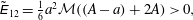 $$\begin{eqnarray}\displaystyle & \tilde{\unicode[STIX]{x1D60C}}_{12}={\textstyle \frac{1}{6}}a^{2}{\mathcal{M}}((A-a)+2A)>0, & \displaystyle\end{eqnarray}$$
 $$\begin{eqnarray}\displaystyle & \tilde{\unicode[STIX]{x1D60C}}_{21}={\textstyle \frac{1}{6}}(2(A-a)^{3}+3{\mathcal{M}}a(A-a)(A+(A-a)+{\mathcal{D}}a))>0, & \displaystyle\end{eqnarray}$$
 $$\begin{eqnarray}\displaystyle & \tilde{\unicode[STIX]{x1D60C}}_{22}={\textstyle \frac{1}{6}}(2(A-a)^{3}+3a{\mathcal{M}}((A-a)+A)(A-a))>0. & \displaystyle\end{eqnarray}$$
The strict inequalities follow since the above entries are sums of positive terms. It follows from this that the trace of
 $\tilde{\boldsymbol{E}}$
is strictly positive. It is also possible to show that the determinant of
$\tilde{\boldsymbol{E}}$
is strictly positive. It is also possible to show that the determinant of
 $\tilde{\unicode[STIX]{x1D640}}$
reduces to
$\tilde{\unicode[STIX]{x1D640}}$
reduces to
 $$\begin{eqnarray}\det (\tilde{\unicode[STIX]{x1D640}})={\textstyle \frac{1}{36}}{\mathcal{M}}Da^{3}(A-a)^{2}(4(A-a)+3{\mathcal{M}}a)>0,\end{eqnarray}$$
where the strict inequality follows from similar arguments as before. Therefore, since both the trace and the determinant of
 $\tilde{\boldsymbol{E}}$
are strictly positive, then
$\tilde{\boldsymbol{E}}$
are strictly positive, then
 $\tilde{\unicode[STIX]{x1D640}}$
must be positive definite.
$\tilde{\unicode[STIX]{x1D640}}$
must be positive definite.
Since all the entries of
 $\tilde{\unicode[STIX]{x1D645}}$
and
$\tilde{\unicode[STIX]{x1D645}}$
and
 $\tilde{\unicode[STIX]{x1D640}}$
are strictly positive, then the trace of
$\tilde{\unicode[STIX]{x1D640}}$
are strictly positive, then the trace of
 $\tilde{\unicode[STIX]{x1D645}}^{\dagger }\tilde{\unicode[STIX]{x1D640}}$
must also be strictly positive. Also note that
$\tilde{\unicode[STIX]{x1D645}}^{\dagger }\tilde{\unicode[STIX]{x1D640}}$
must also be strictly positive. Also note that
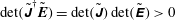 $\det (\tilde{\unicode[STIX]{x1D645}}^{\dagger }\tilde{\boldsymbol{E}})=\det (\tilde{\unicode[STIX]{x1D645}})\det (\tilde{\unicode[STIX]{x1D640}})>0$
. Therefore,
$\det (\tilde{\unicode[STIX]{x1D645}}^{\dagger }\tilde{\boldsymbol{E}})=\det (\tilde{\unicode[STIX]{x1D645}})\det (\tilde{\unicode[STIX]{x1D640}})>0$
. Therefore,
 $\tilde{\unicode[STIX]{x1D645}}^{\dagger }\tilde{\unicode[STIX]{x1D640}}$
is positive definite. The positive definitiveness of
$\tilde{\unicode[STIX]{x1D645}}^{\dagger }\tilde{\unicode[STIX]{x1D640}}$
is positive definite. The positive definitiveness of
 $\tilde{\unicode[STIX]{x1D645}}^{\dagger }\tilde{\unicode[STIX]{x1D63E}}$
follows trivially since
$\tilde{\unicode[STIX]{x1D645}}^{\dagger }\tilde{\unicode[STIX]{x1D63E}}$
follows trivially since
 $\tilde{\unicode[STIX]{x1D63E}}=\unicode[STIX]{x1D63E}\boldsymbol{T}=\unicode[STIX]{x1D644}$
is the identity matrix.
$\tilde{\unicode[STIX]{x1D63E}}=\unicode[STIX]{x1D63E}\boldsymbol{T}=\unicode[STIX]{x1D644}$
is the identity matrix.
Appendix D. Derivation of local equations for perturbations resisted dominantly by vertical shear
For large enough wavenumbers
 $k$
, the perturbations are localised near the lubrication front. Approximating the basic state linearly, that is, to first order in
$k$
, the perturbations are localised near the lubrication front. Approximating the basic state linearly, that is, to first order in
 $\unicode[STIX]{x1D6FF}$
, near the front reduces the mass conservation equations (4.18)–(4.20) to
$\unicode[STIX]{x1D6FF}$
, near the front reduces the mass conservation equations (4.18)–(4.20) to
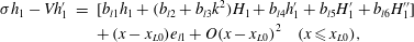 $$\begin{eqnarray}\displaystyle \unicode[STIX]{x1D70E}h_{1}-Vh_{1}^{\prime } & = & \displaystyle [b_{l1}h_{1}+(b_{l2}+b_{l3}k^{2})H_{1}+b_{l4}h_{1}^{\prime }+b_{l5}H_{1}^{\prime }+b_{l6}H_{1}^{\prime \prime }]\nonumber\\ \displaystyle & & \displaystyle +\,(x-x_{L0})e_{l1}+O(x-x_{L0})^{2}\quad (x\leqslant x_{L0}),\end{eqnarray}$$
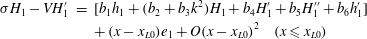 $$\begin{eqnarray}\displaystyle \unicode[STIX]{x1D70E}H_{1}-VH_{1}^{\prime } & = & \displaystyle [b_{1}h_{1}+(b_{2}+b_{3}k^{2})H_{1}+b_{4}H_{1}^{\prime }+b_{5}H_{1}^{\prime \prime }+b_{6}h_{1}^{\prime }]\nonumber\\ \displaystyle & & \displaystyle +\,(x-x_{L0})e_{1}+O(x-x_{L0})^{2}\quad (x\leqslant x_{L0})\end{eqnarray}$$
for the lubricated region and
 $$\begin{eqnarray}\displaystyle \unicode[STIX]{x1D70E}H_{1}-VH_{1}^{\prime } & = & \displaystyle \left(2\unicode[STIX]{x1D6FC}\unicode[STIX]{x1D6FD}^{2}-{\textstyle \frac{1}{3}}\unicode[STIX]{x1D6FC}^{3}k^{2}\right)H_{1}+2\unicode[STIX]{x1D6FC}^{2}\unicode[STIX]{x1D6FD}H_{1}^{\prime }+{\textstyle \frac{1}{3}}\unicode[STIX]{x1D6FC}^{3}H_{1}^{\prime \prime }+(x-x_{L0})e_{2}\nonumber\\ \displaystyle & & \displaystyle +\,O(x-x_{L0})^{2}\quad (x\geqslant x_{L0})\end{eqnarray}$$
for the unlubricated region. Here,
 $b_{li},b_{i}$
, for
$b_{li},b_{i}$
, for
 $i=1,\ldots ,6$
, are functions of the basic-state thicknesses
$i=1,\ldots ,6$
, are functions of the basic-state thicknesses
 $a,A$
, slopes
$a,A$
, slopes
 $b,B$
and viscosity ratio
$b,B$
and viscosity ratio
 ${\mathcal{M}}$
, whereas
${\mathcal{M}}$
, whereas
 $e_{1},e_{l1},e_{2}$
are additionally functions of the perturbed quantities
$e_{1},e_{l1},e_{2}$
are additionally functions of the perturbed quantities
 $h_{1},H_{1}$
and their derivatives, and are listed in (S.7)–(S.21) of the supplementary material. Writing
$h_{1},H_{1}$
and their derivatives, and are listed in (S.7)–(S.21) of the supplementary material. Writing
 $x-x_{L}=\mathit{O}(\unicode[STIX]{x1D6FF})$
, the mass conservation equations locally reduce to the zeroth order (in
$x-x_{L}=\mathit{O}(\unicode[STIX]{x1D6FF})$
, the mass conservation equations locally reduce to the zeroth order (in
 $\unicode[STIX]{x1D6FF}$
) balance of (D 1)–(D 3).
$\unicode[STIX]{x1D6FF}$
) balance of (D 1)–(D 3).
The first-order flux continuity boundary condition
 $$\begin{eqnarray}\left\{c_{1}x_{L1}+\left[c_{2}H_{1}+c_{3}h_{1}+c_{4}\frac{\unicode[STIX]{x2202}H_{1}}{\unicode[STIX]{x2202}x}\right]\right\}^{-}=\left\{c_{5}x_{L1}+\left[c_{6}H_{1}+c_{7}\frac{\unicode[STIX]{x2202}H_{1}}{\unicode[STIX]{x2202}x}\right]\right\}^{+}\end{eqnarray}$$
consists of contributions from flux perturbations as well as from perturbations to the frontal position. Here,
 $c_{1},\ldots ,c_{7}$
are functions of the basic-state thicknesses
$c_{1},\ldots ,c_{7}$
are functions of the basic-state thicknesses
 $h_{0},H_{0}$
and their gradients, as well as
$h_{0},H_{0}$
and their gradients, as well as
 ${\mathcal{M}}$
, and are given in (S.36)–(S.42) of the supplementary material. All quantities are to be evaluated at
${\mathcal{M}}$
, and are given in (S.36)–(S.42) of the supplementary material. All quantities are to be evaluated at
 $x=x_{L0}$
from the side of the lubricated and unlubricated regions as indicated.
$x=x_{L0}$
from the side of the lubricated and unlubricated regions as indicated.
Appendix E. Derivation of local equations for perturbations resisted dominantly by horizontal shear
Near the lubrication front, we locally approximate the basic-state surface heights linearly and find that the governing equation for the upper layer in the lubricated region becomes
 $$\begin{eqnarray}\unicode[STIX]{x1D70E}(H_{1}-h_{1})-V(H_{1}^{\prime }-h_{1}^{\prime })=\unicode[STIX]{x1D709}_{1}H_{1}+\unicode[STIX]{x1D709}_{2}H_{1}^{\prime }+\unicode[STIX]{x1D709}_{3}H_{1}^{\prime \prime }+\unicode[STIX]{x1D709}_{4}h_{1}+\unicode[STIX]{x1D709}_{5}h_{1}^{\prime }\end{eqnarray}$$
and for the lower layer becomes
 $$\begin{eqnarray}\unicode[STIX]{x1D70E}h_{1}-Vh_{1}^{\prime }=\unicode[STIX]{x1D709}_{6}H_{1}+\unicode[STIX]{x1D709}_{7}H_{1}^{\prime }+\unicode[STIX]{x1D709}_{8}H_{1}^{\prime \prime }+\unicode[STIX]{x1D709}_{9}h_{1}+\unicode[STIX]{x1D709}_{10}h_{1}^{\prime },\end{eqnarray}$$
where
 $\unicode[STIX]{x1D709}_{1},\ldots ,\unicode[STIX]{x1D709}_{10}$
are given in (S.78)–(S.87) of the supplementary material.
$\unicode[STIX]{x1D709}_{1},\ldots ,\unicode[STIX]{x1D709}_{10}$
are given in (S.78)–(S.87) of the supplementary material.
After approximating the basic-state surface heights linearly in the unlubricated region, the governing equation reduces to
 $$\begin{eqnarray}\unicode[STIX]{x1D70E}H_{1}-VH_{1}^{\prime }=\left(\frac{1}{2}\unicode[STIX]{x1D6FC}^{2}\unicode[STIX]{x1D6FD}H_{1}^{\prime }+\unicode[STIX]{x1D6FC}\unicode[STIX]{x1D6FD}^{2}H_{1}-\unicode[STIX]{x1D6FC}H_{1}+\frac{1}{k^{2}}(\unicode[STIX]{x1D6FC}H_{1}^{\prime \prime }+\unicode[STIX]{x1D6FD}H_{1}^{\prime })\right)+O(\unicode[STIX]{x1D6FD}(x-x_{L0})).\end{eqnarray}$$
With the local approximation near the front, this further reduces to the zeroth-order form, in
 $x-x_{L0}$
, of the above.
$x-x_{L0}$
, of the above.
E.0.1 Lubrication front
The condition (4.11) of continuity of flux across the lubrication front is given in terms of the perturbation to the combined flux of fluid in the
 $x$
-direction in the lubricated region, which can be written as
$x$
-direction in the lubricated region, which can be written as
 $$\begin{eqnarray}(\boldsymbol{q}_{\mathbf{1}}+\boldsymbol{q}_{\boldsymbol{l}\mathbf{1}})\boldsymbol{\cdot }\boldsymbol{e}_{\boldsymbol{x}}=\frac{1}{2}H_{1}H_{0}^{\prime }(h_{0}^{2}({\mathcal{M}}-1)-2h_{0}H_{0}({\mathcal{M}}-1)-H_{0}^{2})-\frac{1}{k^{2}}H_{1}^{\prime }(h_{0}({\mathcal{M}}-1)+H_{0}),\end{eqnarray}$$
by using the expressions (5.12)–(5.13). Using this and the expression (5.5) for the perturbation to the flux of fluid in the unlubricated region, we find that the flux condition becomes
 $$\begin{eqnarray}\displaystyle & & \displaystyle \left[\frac{1}{2} (\!H_{1}H_{0}^{\prime }(h_{0}^{2}({\mathcal{M}}-1)-2h_{0}H_{0}({\mathcal{M}}-1)-H_{0}^{2})\right.\nonumber\\ \displaystyle & & \displaystyle \qquad -\left.\frac{2}{k^{2}}H_{1}^{\prime }(h_{0}({\mathcal{M}}-1)+H_{0})\!)+\,x_{L1}\frac{\unicode[STIX]{x2202}}{\unicode[STIX]{x2202}x}(\boldsymbol{q}_{\mathbf{0}}+\boldsymbol{q}_{\boldsymbol{l}\mathbf{0}})\boldsymbol{\cdot }\boldsymbol{e}_{\boldsymbol{x}}\right]^{-}\nonumber\\ \displaystyle & & \displaystyle \quad =\left[-\frac{1}{2}\left(H_{0}^{\prime }H_{0}^{2}H_{1}+\frac{2}{k^{2}}H_{0}H_{1}^{\prime }\right)+x_{L1}\frac{\unicode[STIX]{x2202}}{\unicode[STIX]{x2202}x}(\boldsymbol{q}_{\mathbf{0}}\boldsymbol{\cdot }\boldsymbol{e}_{\boldsymbol{x}})\right]^{+}.\end{eqnarray}$$
By using the zeroth-order balance of the mass conservation equations to substitute for the basic-state fluxes and using the local approximation near the front to linearise the basic-state surface heights, we find that the flux condition becomes
 $$\begin{eqnarray}\displaystyle & & \displaystyle \left[\frac{1}{2}BH_{1}(a^{2}({\mathcal{M}}-1)-2aA({\mathcal{M}}-1)-A^{2})-\frac{1}{k^{2}}H_{1}^{\prime }(a({\mathcal{M}}-1)+A)\right]^{-}\nonumber\\ \displaystyle & & \displaystyle \qquad x_{L1}((-a^{2}bB+a^{2}B^{2}+2aAbB-2aAB^{2}-A^{2}bB)({\mathcal{M}}-1)-A^{2}B^{2})\nonumber\\ \displaystyle & & \displaystyle \quad =-\frac{1}{2}\left[\unicode[STIX]{x1D6FD}\unicode[STIX]{x1D6FC}^{2}H_{1}+\frac{2}{k^{2}}\unicode[STIX]{x1D6FC}H_{1}^{\prime }\right]^{+}-\unicode[STIX]{x1D6FC}^{2}\unicode[STIX]{x1D6FD}^{2}x_{L1}\end{eqnarray}$$
for
 $x=x_{L0}$
. The condition of continuity of height gives
$x=x_{L0}$
. The condition of continuity of height gives
 $$\begin{eqnarray}Bx_{L1}+H_{1}^{-}=\unicode[STIX]{x1D6FD}x_{L1}+H_{1}^{+}\end{eqnarray}$$
for
 $x=x_{L0}$
. The kinematic condition gives
$x=x_{L0}$
. The kinematic condition gives
 $$\begin{eqnarray}\displaystyle \unicode[STIX]{x1D70E}x_{L1} & = & \displaystyle \frac{1}{h_{0}^{2}}\left[\left(-x_{L1}h_{0}^{\prime }\boldsymbol{q}_{\boldsymbol{l}\mathbf{0}}\boldsymbol{\cdot }\boldsymbol{e}_{\boldsymbol{x}}+h_{0}x_{L1}\frac{\unicode[STIX]{x2202}}{\unicode[STIX]{x2202}x}\boldsymbol{q}_{\boldsymbol{l}\mathbf{0}}\boldsymbol{\cdot }\boldsymbol{e}_{\boldsymbol{x}}-h_{1}\boldsymbol{q}_{\boldsymbol{l}\mathbf{0}}\boldsymbol{\cdot }\boldsymbol{e}_{\boldsymbol{x}}\right)\right.\nonumber\\ \displaystyle & & \displaystyle +\,\frac{1}{2}\left(h_{0}^{3}(H_{1}-h_{1}){\mathcal{M}}H_{0}^{\prime }-h_{0}^{3}H_{1}H_{0}^{\prime }-2h_{0}^{2}H_{0}(H_{1}-h_{1}){\mathcal{M}}H_{0}^{\prime }\right.\nonumber\\ \displaystyle & & \displaystyle +\left.\left.2h_{0}^{2}H_{0}H_{1}H_{0}^{\prime }-h_{0}H_{0}^{2}H_{1}H_{0}^{\prime }-\frac{2}{k^{2}}h_{0}(H_{0}-h_{0})H_{1}^{\prime }\right)\right]\end{eqnarray}$$
for
 $x=x_{L0}^{-}$
. Using zeroth-order balances, we substitute for the basic-state flux, apply the linear approximation for the surface heights near the front and find the local kinematic condition
$x=x_{L0}^{-}$
. Using zeroth-order balances, we substitute for the basic-state flux, apply the linear approximation for the surface heights near the front and find the local kinematic condition
 $$\begin{eqnarray}\displaystyle \unicode[STIX]{x1D70E}x_{L1} & = & \displaystyle \frac{1}{6a^{2}}\left[\vphantom{\frac{6}{k^{2}}} (\!3a^{2}{\mathcal{M}}(-2ab+3aB+3Ab-4AB)+2(a-A)^{2} (\!2ab\right.\nonumber\\ \displaystyle & & \displaystyle -\,3aB+Ab\!)\!)Bx_{L1}+ ((-3aA{\mathcal{M}}(a-2A)-2(a-A)^{3})Bh_{1}\nonumber\\ \displaystyle & & \displaystyle +\left.3(a{\mathcal{M}}(a-2A)-(a-A)^{2})aBH_{1}\! )+\frac{6}{k^{2}}a(a-A)H_{1}^{\prime }\right]\end{eqnarray}$$
for
 $x=x_{L0}^{-}$
.
$x=x_{L0}^{-}$
.
E.0.2 Dispersion relation
The mass conservation equations (E 3), (E 1)–(E 2) along with the height, flux and kinematic conditions (E 6)–(E 7), (E 9) form a system of linear differential equations with solutions
 $$\begin{eqnarray}\displaystyle & (h_{1},H_{1})=(\tilde{h}_{1}^{-},\tilde{H}_{1}^{-})\exp ((x-x_{L0})\unicode[STIX]{x1D706}^{-})\quad (x\leqslant x_{L0}), & \displaystyle\end{eqnarray}$$
 $$\begin{eqnarray}\displaystyle & H_{1}=\tilde{H}_{1}^{+}\exp ((x-x_{L0})\unicode[STIX]{x1D706}^{+})\quad (x\geqslant x_{L0}), & \displaystyle\end{eqnarray}$$
 $\tilde{h}_{1}^{-}$
,
$\tilde{h}_{1}^{-}$
,
 $\tilde{H}_{1}^{-}$
and
$\tilde{H}_{1}^{-}$
and
 $\tilde{H}_{1}^{+}$
are constants, after non-dimensionalising by using the length and time scales found in (2.2). Direct substitution into the dimensionless versions of the mass conservation equations (E 3), (E 1)–(E 2) and boundary conditions (E 6)–(E 7), (E 9) gives the following governing equation for the unlubricated region:
$\tilde{H}_{1}^{+}$
are constants, after non-dimensionalising by using the length and time scales found in (2.2). Direct substitution into the dimensionless versions of the mass conservation equations (E 3), (E 1)–(E 2) and boundary conditions (E 6)–(E 7), (E 9) gives the following governing equation for the unlubricated region:  $$\begin{eqnarray}\unicode[STIX]{x1D70E}-V\unicode[STIX]{x1D706}^{+}=\frac{1}{2}\unicode[STIX]{x1D6FC}^{2}\unicode[STIX]{x1D6FD}\unicode[STIX]{x1D706}^{+}+\unicode[STIX]{x1D6FC}\unicode[STIX]{x1D6FD}^{2}-\unicode[STIX]{x1D6FC}+\frac{1}{k^{2}}(\unicode[STIX]{x1D6FC}(\unicode[STIX]{x1D706}^{+})^{2}+\unicode[STIX]{x1D6FD}\unicode[STIX]{x1D706}^{+}),\end{eqnarray}$$
and for the upper layer of the lubricated region
 $$\begin{eqnarray}\displaystyle (\unicode[STIX]{x1D70E}-V\unicode[STIX]{x1D706}^{-})(\tilde{H}_{1}^{-}-\tilde{h}_{1}^{-})=(\unicode[STIX]{x1D712}_{1}+\unicode[STIX]{x1D712}_{2}\unicode[STIX]{x1D706}^{-})\tilde{h}_{1}^{-}+(\unicode[STIX]{x1D712}_{3}+\unicode[STIX]{x1D712}_{4}\unicode[STIX]{x1D706}^{-}+\unicode[STIX]{x1D712}_{5}(\unicode[STIX]{x1D706}^{-})^{2})\tilde{H}_{1}^{-} & & \displaystyle\end{eqnarray}$$
and lower layer of the lubricated region
 $$\begin{eqnarray}\displaystyle (\unicode[STIX]{x1D70E}-V\unicode[STIX]{x1D706}^{-})\tilde{h}_{1}^{-}=(\unicode[STIX]{x1D712}_{l1}+\unicode[STIX]{x1D712}_{l2}\unicode[STIX]{x1D706}^{-})\tilde{h}_{1}^{-}+(\unicode[STIX]{x1D712}_{l3}+\unicode[STIX]{x1D712}_{l4}\unicode[STIX]{x1D706}^{-}+\unicode[STIX]{x1D712}_{l5}(\unicode[STIX]{x1D706}^{-})^{2})\tilde{H}_{1}^{-}, & & \displaystyle\end{eqnarray}$$
where
 $\unicode[STIX]{x1D712}_{1},\ldots ,\unicode[STIX]{x1D712}_{5}$
and
$\unicode[STIX]{x1D712}_{1},\ldots ,\unicode[STIX]{x1D712}_{5}$
and
 $\unicode[STIX]{x1D712}_{l1},\ldots ,\unicode[STIX]{x1D712}_{l5}$
are given in (S.88)–(S.92) and (S.100)–(S.104) of the supplementary material.
$\unicode[STIX]{x1D712}_{l1},\ldots ,\unicode[STIX]{x1D712}_{l5}$
are given in (S.88)–(S.92) and (S.100)–(S.104) of the supplementary material.
The flux continuity condition gives
 $$\begin{eqnarray}\unicode[STIX]{x1D712}_{6}\tilde{H}_{1}^{-}+\unicode[STIX]{x1D712}_{7}\unicode[STIX]{x1D706}^{-}\tilde{H}_{1}^{-}+\unicode[STIX]{x1D712}_{8}x_{L1}=-\frac{1}{2}\left(\unicode[STIX]{x1D6FD}\unicode[STIX]{x1D6FC}^{2}\tilde{H}_{1}^{+}+\frac{2}{k^{2}}\unicode[STIX]{x1D6FC}\unicode[STIX]{x1D706}^{+}\tilde{H}_{1}^{+}\right)-\unicode[STIX]{x1D6FC}^{2}\unicode[STIX]{x1D6FD}^{2}x_{L1}\end{eqnarray}$$
and height continuity gives
 $$\begin{eqnarray}Bx_{L1}+\tilde{H}_{1}^{-}=\unicode[STIX]{x1D6FD}x_{L1}+\tilde{H}_{1}^{+}.\end{eqnarray}$$
The kinematic condition becomes
 $$\begin{eqnarray}\displaystyle \unicode[STIX]{x1D70E}x_{L1}=\unicode[STIX]{x1D712}_{9}\tilde{h}_{1}^{-}+\unicode[STIX]{x1D712}_{10}\tilde{H}_{1}^{-}+\unicode[STIX]{x1D712}_{11}\unicode[STIX]{x1D706}^{-}\tilde{H}_{1}^{-}+\unicode[STIX]{x1D712}_{12}x_{L1}, & & \displaystyle\end{eqnarray}$$
where
 $\unicode[STIX]{x1D712}_{6},\ldots ,\unicode[STIX]{x1D712}_{12}$
are given in (S.93)–(S.99) of the supplementary material.
$\unicode[STIX]{x1D712}_{6},\ldots ,\unicode[STIX]{x1D712}_{12}$
are given in (S.93)–(S.99) of the supplementary material.
The mass conservation equations (E 11), (E 12)–(E 13) and height, flux and kinematic conditions (E 14)–(E 15), (E 16) are a system of six equations for six unknown variables
 $\unicode[STIX]{x1D70E},x_{L1},\tilde{h}_{1}^{-},\tilde{H}_{1}^{+},\unicode[STIX]{x1D706}^{-},\unicode[STIX]{x1D706}^{+}$
, where, as before, we set
$\unicode[STIX]{x1D70E},x_{L1},\tilde{h}_{1}^{-},\tilde{H}_{1}^{+},\unicode[STIX]{x1D706}^{-},\unicode[STIX]{x1D706}^{+}$
, where, as before, we set
 $\tilde{H}_{1}^{-}\equiv 1$
, without loss of generality. The choice of solutions is restricted to those that satisfy decay conditions away from the lubrication front, that is, it is required that
$\tilde{H}_{1}^{-}\equiv 1$
, without loss of generality. The choice of solutions is restricted to those that satisfy decay conditions away from the lubrication front, that is, it is required that
 $\unicode[STIX]{x1D706}^{-}>0$
and
$\unicode[STIX]{x1D706}^{-}>0$
and
 $\unicode[STIX]{x1D706}^{+}<0$
.
$\unicode[STIX]{x1D706}^{+}<0$
.
E.0.3 Large-
$k$
asymptotics

The mass conservation equations for the lubricated region can be written in matrix form
 $$\begin{eqnarray}(\unicode[STIX]{x1D64B}-(\unicode[STIX]{x1D70E}-V\unicode[STIX]{x1D706}^{-})\unicode[STIX]{x1D644})[\tilde{h}_{1}^{-},\tilde{H}_{1}^{-}]^{\text{T}}=\mathbf{0},\end{eqnarray}$$
where the entries of the matrix
 $\unicode[STIX]{x1D64B}$
are
$\unicode[STIX]{x1D64B}$
are
 $$\begin{eqnarray}\left.\begin{array}{@{}c@{}}\unicode[STIX]{x1D617}_{11}=\left(Ab-{\textstyle \frac{1}{2}}a^{2}\unicode[STIX]{x1D706}^{-}+a(B-b+A\unicode[STIX]{x1D706}^{-})\right)B{\mathcal{M}},\\ \unicode[STIX]{x1D617}_{12}=\left({\displaystyle \frac{1}{k^{2}}}(b\unicode[STIX]{x1D706}^{-}+a(\unicode[STIX]{x1D706}^{-})^{2})-a\right){\mathcal{M}},\\ \unicode[STIX]{x1D617}_{21}=0,\\ \unicode[STIX]{x1D617}_{22}=(a-A)-(A-a)bB+(A-a)B^{2}-aM+(A-a)bBM\\ \quad \qquad +\,aB^{2}M+\unicode[STIX]{x1D706}^{-}\left(-{\textstyle \frac{1}{2}}a^{2}B(M-1)+aAB(M-1)+{\textstyle \frac{1}{2}}A^{2}B\right)\\ \quad \qquad +\,{\displaystyle \frac{1}{k^{2}}}((A-a)(\unicode[STIX]{x1D706}^{-})^{2}+(B-b)\unicode[STIX]{x1D706}^{-}+b\unicode[STIX]{x1D706}^{-}M+a(\unicode[STIX]{x1D706}^{-})^{2}M).\end{array}\right\}\end{eqnarray}$$
For non-trivial solutions, it is necessary that
 $$\begin{eqnarray}\det (\unicode[STIX]{x1D64B}-(\unicode[STIX]{x1D70E}-V\unicode[STIX]{x1D706}^{-})\unicode[STIX]{x1D644})=0\end{eqnarray}$$
giving a cubic equation for
 $\unicode[STIX]{x1D706}^{-}$
. Expanding in series of
$\unicode[STIX]{x1D706}^{-}$
. Expanding in series of
 $1/k$
for
$1/k$
for
 $k$
large,
$k$
large,
 $$\begin{eqnarray}\left.\begin{array}{@{}c@{}}\unicode[STIX]{x1D70E}=\unicode[STIX]{x1D70E}_{1}+\unicode[STIX]{x1D70E}_{2}/k+\cdots \,,\\ \unicode[STIX]{x1D706}^{\pm }=\unicode[STIX]{x1D706}_{-1}^{\pm }k^{2}+\unicode[STIX]{x1D706}_{0}^{\pm }k+\cdots \,,\\ \tilde{H}_{1}^{\pm }=\tilde{H}_{10}^{\pm }k+\tilde{H}_{11}^{\pm }+\cdots \,,\\ \tilde{h}_{1}^{-}=\tilde{h}_{11}^{-}+k^{-1}\tilde{h}_{12}^{-}+\cdots \,,\\ x_{L1}=x_{L11}+k^{-1}x_{L12}+\cdots \,,\end{array}\right\}\end{eqnarray}$$
gives that the leading-order behaviour of the root
 $\unicode[STIX]{x1D706}^{-}$
is
$\unicode[STIX]{x1D706}^{-}$
is
 $$\begin{eqnarray}\displaystyle \unicode[STIX]{x1D706}^{-}=\frac{-(a-A)^{2}B+a(a-2A)B{\mathcal{M}}-2V}{2(A+a({\mathcal{M}}-1))}k^{2}+O(k) & & \displaystyle\end{eqnarray}$$
so that
 $\unicode[STIX]{x1D706}_{-1}^{-}$
can be read from the leading-order term above. Here, we exclude solutions for which
$\unicode[STIX]{x1D706}_{-1}^{-}$
can be read from the leading-order term above. Here, we exclude solutions for which
 $\unicode[STIX]{x1D706}^{-}<0$
. The relationship between
$\unicode[STIX]{x1D706}^{-}<0$
. The relationship between
 $\tilde{h}_{1}^{-}$
and
$\tilde{h}_{1}^{-}$
and
 $\tilde{H}_{1}^{-}$
can be determined from the equation of mass conservation for the lower layer to be
$\tilde{H}_{1}^{-}$
can be determined from the equation of mass conservation for the lower layer to be
 $$\begin{eqnarray}\displaystyle \tilde{h}_{1}^{-}=\frac{a{\mathcal{M}}(-(a-A)^{2}B+a(a-2A)B{\mathcal{M}}-2V)}{(A+a({\mathcal{M}}-1))(a(a-2A)B{\mathcal{M}}-2V)}+O(1/k) & & \displaystyle\end{eqnarray}$$
so that
 $\tilde{h}_{11}^{-}$
can be read from the leading-order term above. Here, recall that
$\tilde{h}_{11}^{-}$
can be read from the leading-order term above. Here, recall that
 $\tilde{H}_{1}^{-}=1$
, without loss of generality. By solving the mass conservation equation for the unlubricated region for
$\tilde{H}_{1}^{-}=1$
, without loss of generality. By solving the mass conservation equation for the unlubricated region for
 $\unicode[STIX]{x1D706}^{+}$
, excluding the positive root and expanding in series of
$\unicode[STIX]{x1D706}^{+}$
, excluding the positive root and expanding in series of
 $1/k$
, we find the leading-order behaviour of
$1/k$
, we find the leading-order behaviour of
 $\unicode[STIX]{x1D706}^{+}$
to be
$\unicode[STIX]{x1D706}^{+}$
to be
 $$\begin{eqnarray}\unicode[STIX]{x1D706}^{+}=\frac{2(-\unicode[STIX]{x1D6FC}\unicode[STIX]{x1D6FD}^{2}+\unicode[STIX]{x1D6FC}+\unicode[STIX]{x1D70E}_{1})}{\unicode[STIX]{x1D6FC}^{2}\unicode[STIX]{x1D6FD}+2V}+O(1/k),\end{eqnarray}$$
which tends to a constant as
 $k\rightarrow \infty$
. Expanding the kinematic condition in series of
$k\rightarrow \infty$
. Expanding the kinematic condition in series of
 $1/k$
gives the leading-order behaviour of
$1/k$
gives the leading-order behaviour of
 $x_{L1}$
to be
$x_{L1}$
to be
 $$\begin{eqnarray}\displaystyle x_{L1}=\frac{\unicode[STIX]{x1D711}_{1}\tilde{H}_{1}^{-}+\unicode[STIX]{x1D711}_{2}\tilde{h}_{1}^{-}}{\unicode[STIX]{x1D711}_{3}}+O(1/k), & & \displaystyle\end{eqnarray}$$
which depends on the relation between
 $\tilde{h}_{1}^{-}$
and
$\tilde{h}_{1}^{-}$
and
 $\tilde{H}_{1}^{-}$
, where
$\tilde{H}_{1}^{-}$
, where
 $\unicode[STIX]{x1D711}_{i}$
are given in (S.106)–(S.115) of the supplementary material. Using (E 22) to substitute for the value of
$\unicode[STIX]{x1D711}_{i}$
are given in (S.106)–(S.115) of the supplementary material. Using (E 22) to substitute for the value of
 $\tilde{h}_{1}^{-}$
and expanding in series of
$\tilde{h}_{1}^{-}$
and expanding in series of
 $1/k$
gives the leading-order behaviour for
$1/k$
gives the leading-order behaviour for
 $x_{L1}$
to be
$x_{L1}$
to be
 $$\begin{eqnarray}\displaystyle x_{L1}=\frac{\unicode[STIX]{x1D711}_{4}}{\unicode[STIX]{x1D711}_{5}}+O(1/k). & & \displaystyle\end{eqnarray}$$
Therefore,
 $x_{L1}$
tends to a constant as
$x_{L1}$
tends to a constant as
 $k\rightarrow \infty$
. Height continuity gives the value of
$k\rightarrow \infty$
. Height continuity gives the value of
 $\tilde{H}_{1}^{+}$
as
$\tilde{H}_{1}^{+}$
as
 $$\begin{eqnarray}\tilde{H}_{1}^{+}=\tilde{H}_{1}^{-}+(B-\unicode[STIX]{x1D6FD})x_{L1}.\end{eqnarray}$$
Substituting this into the condition of flux continuity gives an alternative expression for
 $x_{L1}$
as
$x_{L1}$
as
 $$\begin{eqnarray}\displaystyle x_{L1}=\frac{\unicode[STIX]{x1D711}_{6}}{\unicode[STIX]{x1D711}_{7}}\tilde{H}_{1}^{-}+O(1/k). & & \displaystyle\end{eqnarray}$$
Comparing this with the previous expression (E 25) for
 $x_{L1}$
gives an implicit dispersion relation for
$x_{L1}$
gives an implicit dispersion relation for
 $\unicode[STIX]{x1D70E}$
. The explicit dispersion relation for
$\unicode[STIX]{x1D70E}$
. The explicit dispersion relation for
 $\unicode[STIX]{x1D70E}$
, in the large-
$\unicode[STIX]{x1D70E}$
, in the large-
 $k$
limit, involves over 300 terms and is not written here for conciseness. The large-
$k$
limit, involves over 300 terms and is not written here for conciseness. The large-
 $k$
behaviour of
$k$
behaviour of
 $\unicode[STIX]{x1D70E}$
, in the limit of
$\unicode[STIX]{x1D70E}$
, in the limit of
 $M\rightarrow \infty$
, is given by
$M\rightarrow \infty$
, is given by
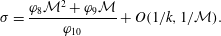 $$\begin{eqnarray}\displaystyle \unicode[STIX]{x1D70E}=\frac{\unicode[STIX]{x1D711}_{8}{\mathcal{M}}^{2}+\unicode[STIX]{x1D711}_{9}{\mathcal{M}}}{\unicode[STIX]{x1D711}_{10}}+O(1/k,1/{\mathcal{M}}). & & \displaystyle\end{eqnarray}$$
Appendix F. Derivation of local equations for perturbations resisted by horizontal and vertical shear
F.1 Unlubricated region
The perturbed velocity components in the
 $x$
- and
$x$
- and
 $y$
-directions are given by
$y$
-directions are given by
 $$\begin{eqnarray}\displaystyle & \displaystyle u_{1}=\frac{2}{k^{2}}\sinh \left(\frac{kz}{2}\right)\text{sech}(kH_{0})\left[\frac{\unicode[STIX]{x2202}H_{1}}{\unicode[STIX]{x2202}x}\sinh \left(\frac{1}{2}k(z-2H_{0})\right)+-k\cosh \left(\frac{kz}{2}\right)H_{1}\frac{\unicode[STIX]{x2202}H_{0}}{\unicode[STIX]{x2202}x}\right], & \displaystyle \nonumber\\ \displaystyle & & \displaystyle\end{eqnarray}$$
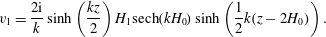 $$\begin{eqnarray}\displaystyle & \displaystyle v_{1}=\frac{2\text{i}}{k}\sinh \left(\frac{kz}{2}\right)H_{1}\text{sech}(kH_{0})\sinh \left(\frac{1}{2}k(z-2H_{0})\right). & \displaystyle\end{eqnarray}$$
The components of the perturbation to the volume flux, per unit width, given by (5.4), can be found to be given by
 $$\begin{eqnarray}q_{u1}=\frac{1}{2k^{3}}\left[2(\tanh (kH_{0})-kH_{0})\frac{\unicode[STIX]{x2202}H_{1}}{\unicode[STIX]{x2202}x}-kH_{1}(k^{2}H_{0}^{2}+-2\text{sech}(kH_{0})+2)\frac{\unicode[STIX]{x2202}H_{0}}{\unicode[STIX]{x2202}x}\right]\end{eqnarray}$$
and
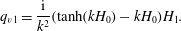 $$\begin{eqnarray}\displaystyle q_{v1}=\frac{\text{i}}{k^{2}}(\tanh (kH_{0})-kH_{0})H_{1}. & & \displaystyle\end{eqnarray}$$
The mass conservation equation for perturbations at the next order in
 $\unicode[STIX]{x1D716}$
gives
$\unicode[STIX]{x1D716}$
gives
 $$\begin{eqnarray}\displaystyle \unicode[STIX]{x1D70E}H_{1}-V\frac{\unicode[STIX]{x2202}H_{1}}{\unicode[STIX]{x2202}x} & = & \displaystyle -\unicode[STIX]{x1D735}\boldsymbol{\cdot }\boldsymbol{q}_{\mathbf{1}}\nonumber\\ \displaystyle & = & \displaystyle -\frac{\unicode[STIX]{x2202}}{\unicode[STIX]{x2202}x}(\boldsymbol{q}_{\mathbf{1}}\boldsymbol{\cdot }\boldsymbol{e}_{\boldsymbol{x}})-\text{i}k\boldsymbol{q}_{\mathbf{1}}\boldsymbol{\cdot }\boldsymbol{e}_{\boldsymbol{y}}.\end{eqnarray}$$
By non-dimensionalising and approximating the basic-state surface heights piecewise linearly by (4.15) and assuming that the changes in surface slope,
 $\unicode[STIX]{x1D6FF}(\unicode[STIX]{x2202}H_{0}/\unicode[STIX]{x2202}x)$
, are small in the vicinity of the lubrication front, the mass conservation equation for the unlubricated region reduces to
$\unicode[STIX]{x1D6FF}(\unicode[STIX]{x2202}H_{0}/\unicode[STIX]{x2202}x)$
, are small in the vicinity of the lubrication front, the mass conservation equation for the unlubricated region reduces to
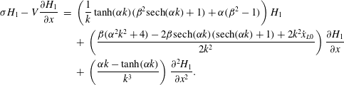 $$\begin{eqnarray}\displaystyle \unicode[STIX]{x1D70E}H_{1}-V\frac{\unicode[STIX]{x2202}H_{1}}{\unicode[STIX]{x2202}x} & = & \displaystyle \left(\frac{1}{k}\tanh (\unicode[STIX]{x1D6FC}k)(\unicode[STIX]{x1D6FD}^{2}\text{sech}(\unicode[STIX]{x1D6FC}k)+1)+\unicode[STIX]{x1D6FC}(\unicode[STIX]{x1D6FD}^{2}-1)\right)H_{1}\nonumber\\ \displaystyle & & \displaystyle +\,\left(\frac{\unicode[STIX]{x1D6FD}(\unicode[STIX]{x1D6FC}^{2}k^{2}+4)-2\unicode[STIX]{x1D6FD}\text{sech}(\unicode[STIX]{x1D6FC}k)(\text{sech}(\unicode[STIX]{x1D6FC}k)+1)+2k^{2}{\dot{x}}_{L0}}{2k^{2}}\right)\frac{\unicode[STIX]{x2202}H_{1}}{\unicode[STIX]{x2202}x}\nonumber\\ \displaystyle & & \displaystyle +\,\left(\frac{\unicode[STIX]{x1D6FC}k-\tanh (\unicode[STIX]{x1D6FC}k)}{k^{3}}\right)\frac{\unicode[STIX]{x2202}^{2}H_{1}}{\unicode[STIX]{x2202}x^{2}}.\end{eqnarray}$$
F.2 Lubricated region
The
 $x$
- and
$x$
- and
 $y$
-components of the perturbed velocity field in the upper layer may be written as
$y$
-components of the perturbed velocity field in the upper layer may be written as
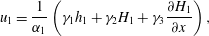 $$\begin{eqnarray}\displaystyle & \displaystyle u_{1}=\frac{1}{\unicode[STIX]{x1D6FC}_{1}}\left(\unicode[STIX]{x1D6FE}_{1}h_{1}+\unicode[STIX]{x1D6FE}_{2}H_{1}+\unicode[STIX]{x1D6FE}_{3}\frac{\unicode[STIX]{x2202}H_{1}}{\unicode[STIX]{x2202}x}\right), & \displaystyle\end{eqnarray}$$
 $$\begin{eqnarray}\displaystyle & \displaystyle v_{1}=\text{i}\frac{\unicode[STIX]{x1D6FE}_{4}}{\unicode[STIX]{x1D6FC}_{1}}H_{1}, & \displaystyle\end{eqnarray}$$
where the coefficients are given in (S.116)–(S.120) of the supplementary material.
The
 $x$
- and
$x$
- and
 $y$
-components of the perturbed velocity field in the lower layer are
$y$
-components of the perturbed velocity field in the lower layer are
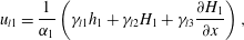 $$\begin{eqnarray}\displaystyle & \displaystyle u_{l1}=\frac{1}{\unicode[STIX]{x1D6FC}_{1}}\left(\unicode[STIX]{x1D6FE}_{l1}h_{1}+\unicode[STIX]{x1D6FE}_{l2}H_{1}+\unicode[STIX]{x1D6FE}_{l3}\frac{\unicode[STIX]{x2202}H_{1}}{\unicode[STIX]{x2202}x}\right), & \displaystyle\end{eqnarray}$$
 $$\begin{eqnarray}\displaystyle & \displaystyle v_{l1}=\text{i}\frac{\unicode[STIX]{x1D6FE}_{l4}}{\unicode[STIX]{x1D6FC}_{1}}H_{1}, & \displaystyle\end{eqnarray}$$
where
 $\unicode[STIX]{x1D6FE}_{li}$
are given in (S.121)–(S.124) of the supplementary material.
$\unicode[STIX]{x1D6FE}_{li}$
are given in (S.121)–(S.124) of the supplementary material.
The components of the depth-integrated volume flux, per unit width, for the upper layer are
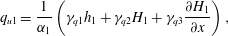 $$\begin{eqnarray}\displaystyle & \displaystyle q_{u1}=\frac{1}{\unicode[STIX]{x1D6FC}_{1}}\left(\unicode[STIX]{x1D6FE}_{q1}h_{1}+\unicode[STIX]{x1D6FE}_{q2}H_{1}+\unicode[STIX]{x1D6FE}_{q3}\frac{\unicode[STIX]{x2202}H_{1}}{\unicode[STIX]{x2202}x}\right), & \displaystyle\end{eqnarray}$$
 $$\begin{eqnarray}\displaystyle & \displaystyle v_{1}=\text{i}\frac{\unicode[STIX]{x1D6FE}_{q4}}{\unicode[STIX]{x1D6FC}_{1}}H_{1}, & \displaystyle\end{eqnarray}$$
where
 $\unicode[STIX]{x1D6FE}_{qi}$
are given in (S.125)–(S.128) of the supplementary material.
$\unicode[STIX]{x1D6FE}_{qi}$
are given in (S.125)–(S.128) of the supplementary material.
Conservation of mass at first order in
 $\unicode[STIX]{x1D716}$
is given by
$\unicode[STIX]{x1D716}$
is given by
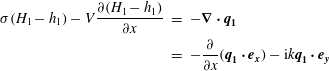 $$\begin{eqnarray}\displaystyle \unicode[STIX]{x1D70E}(H_{1}-h_{1})-V\frac{\unicode[STIX]{x2202}(H_{1}-h_{1})}{\unicode[STIX]{x2202}x} & = & \displaystyle -\unicode[STIX]{x1D735}\boldsymbol{\cdot }\boldsymbol{q}_{\mathbf{1}}\nonumber\\ \displaystyle & = & \displaystyle -\frac{\unicode[STIX]{x2202}}{\unicode[STIX]{x2202}x}(\boldsymbol{q}_{\mathbf{1}}\boldsymbol{\cdot }\boldsymbol{e}_{\boldsymbol{x}})-\text{i}k\boldsymbol{q}_{\mathbf{1}}\boldsymbol{\cdot }\boldsymbol{e}_{\boldsymbol{y}}\end{eqnarray}$$
for the upper layer and
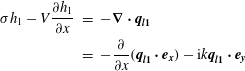 $$\begin{eqnarray}\displaystyle \unicode[STIX]{x1D70E}h_{1}-V\frac{\unicode[STIX]{x2202}h_{1}}{\unicode[STIX]{x2202}x} & = & \displaystyle -\unicode[STIX]{x1D735}\boldsymbol{\cdot }\boldsymbol{q}_{\boldsymbol{l}\mathbf{1}}\nonumber\\ \displaystyle & = & \displaystyle -\frac{\unicode[STIX]{x2202}}{\unicode[STIX]{x2202}x}(\boldsymbol{q}_{\boldsymbol{l}\mathbf{1}}\boldsymbol{\cdot }\boldsymbol{e}_{\boldsymbol{x}})-\text{i}k\boldsymbol{q}_{\boldsymbol{l}\mathbf{1}}\boldsymbol{\cdot }\boldsymbol{e}_{\boldsymbol{y}}\end{eqnarray}$$
for the lower layer.
In what follows, we approximate the basic-state surface heights piecewise linearly by (4.15) and also assume that the changes in surface slope,
 $\unicode[STIX]{x1D6FF}(\unicode[STIX]{x2202}H_{0}/\unicode[STIX]{x2202}x)$
and
$\unicode[STIX]{x1D6FF}(\unicode[STIX]{x2202}H_{0}/\unicode[STIX]{x2202}x)$
and
 $\unicode[STIX]{x1D6FF}(\unicode[STIX]{x2202}h_{0}/\unicode[STIX]{x2202}x)$
, of the two layers are small in the vicinity of the lubrication front. After non-dimensionalising, this reduces the mass conservation equation for the upper layer to
$\unicode[STIX]{x1D6FF}(\unicode[STIX]{x2202}h_{0}/\unicode[STIX]{x2202}x)$
, of the two layers are small in the vicinity of the lubrication front. After non-dimensionalising, this reduces the mass conservation equation for the upper layer to
 $$\begin{eqnarray}\unicode[STIX]{x1D70E}(H_{1}-h_{1})-V\frac{\unicode[STIX]{x2202}(H_{1}-h_{1})}{\unicode[STIX]{x2202}x}=\unicode[STIX]{x1D6FD}_{1}h_{1}+\unicode[STIX]{x1D6FD}_{2}H_{1}+\unicode[STIX]{x1D6FD}_{3}\frac{\unicode[STIX]{x2202}h_{1}}{\unicode[STIX]{x2202}x}+\unicode[STIX]{x1D6FD}_{4}\frac{\unicode[STIX]{x2202}H_{1}}{\unicode[STIX]{x2202}x}+\unicode[STIX]{x1D6FD}_{5}\frac{\unicode[STIX]{x2202}^{2}H_{1}}{\unicode[STIX]{x2202}x^{2}},\end{eqnarray}$$
where the coefficients
 $\unicode[STIX]{x1D6FD}_{1},\ldots ,\unicode[STIX]{x1D6FD}_{5}$
depend on the basic-state thicknesses and surface slopes as well as the wavenumber and are given in (S.129)–(S.133) of the supplementary material. Similarly, the mass conservation equation for the lower layer reduces to
$\unicode[STIX]{x1D6FD}_{1},\ldots ,\unicode[STIX]{x1D6FD}_{5}$
depend on the basic-state thicknesses and surface slopes as well as the wavenumber and are given in (S.129)–(S.133) of the supplementary material. Similarly, the mass conservation equation for the lower layer reduces to
 $$\begin{eqnarray}\displaystyle \unicode[STIX]{x1D70E}h_{1}-V\frac{\unicode[STIX]{x2202}h_{1}}{\unicode[STIX]{x2202}x}=\unicode[STIX]{x1D6FD}_{l1}h_{1}+\unicode[STIX]{x1D6FD}_{l2}H_{1}+\unicode[STIX]{x1D6FD}_{l3}\frac{\unicode[STIX]{x2202}h_{1}}{\unicode[STIX]{x2202}x}+\unicode[STIX]{x1D6FD}_{l4}\frac{\unicode[STIX]{x2202}H_{1}}{\unicode[STIX]{x2202}x}+\unicode[STIX]{x1D6FD}_{l5}\frac{\unicode[STIX]{x2202}^{2}H_{1}}{\unicode[STIX]{x2202}x^{2}}. & & \displaystyle\end{eqnarray}$$
The coefficients
 $\unicode[STIX]{x1D6FD}_{l1},\ldots ,\unicode[STIX]{x1D6FD}_{l5}$
are given in (S.135)–(S.139) of the supplementary material.
$\unicode[STIX]{x1D6FD}_{l1},\ldots ,\unicode[STIX]{x1D6FD}_{l5}$
are given in (S.135)–(S.139) of the supplementary material.
F.3 Lubrication front
The condition (4.11) of continuity of flux across the lubrication front gives
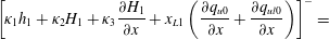 $$\begin{eqnarray}\displaystyle & \displaystyle \left[\unicode[STIX]{x1D705}_{1}h_{1}+\unicode[STIX]{x1D705}_{2}H_{1}+\unicode[STIX]{x1D705}_{3}\frac{\unicode[STIX]{x2202}H_{1}}{\unicode[STIX]{x2202}x}+x_{L1}\left(\frac{\unicode[STIX]{x2202}q_{u0}}{\unicode[STIX]{x2202}x}+\frac{\unicode[STIX]{x2202}q_{ul0}}{\unicode[STIX]{x2202}x}\right)\right]^{-}= & \displaystyle\end{eqnarray}$$
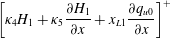 $$\begin{eqnarray}\displaystyle & \displaystyle \left[\unicode[STIX]{x1D705}_{4}H_{1}+\unicode[STIX]{x1D705}_{5}\frac{\unicode[STIX]{x2202}H_{1}}{\unicode[STIX]{x2202}x}+x_{L1}\frac{\unicode[STIX]{x2202}q_{u0}}{\unicode[STIX]{x2202}x}\right]^{+} & \displaystyle\end{eqnarray}$$
at
 $x=x_{L0}$
, where the coefficients
$x=x_{L0}$
, where the coefficients
 $\unicode[STIX]{x1D705}_{1},\ldots ,\unicode[STIX]{x1D705}_{5}$
are given in terms of the basic-state thicknesses and surface gradients at the lubrication front, and are specified in (S.140)–(S.144) of the supplementary material.
$\unicode[STIX]{x1D705}_{1},\ldots ,\unicode[STIX]{x1D705}_{5}$
are given in terms of the basic-state thicknesses and surface gradients at the lubrication front, and are specified in (S.140)–(S.144) of the supplementary material.
Continuity of height gives
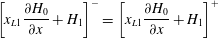 $$\begin{eqnarray}\displaystyle \left[x_{L1}\frac{\unicode[STIX]{x2202}H_{0}}{\unicode[STIX]{x2202}x}+H_{1}\right]^{-}=\left[x_{L1}\frac{\unicode[STIX]{x2202}H_{0}}{\unicode[STIX]{x2202}x}+H_{1}\right]^{+} & & \displaystyle\end{eqnarray}$$
at
 $x=x_{L0}$
. The kinematic condition reduces to
$x=x_{L0}$
. The kinematic condition reduces to
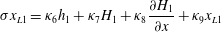 $$\begin{eqnarray}\displaystyle \unicode[STIX]{x1D70E}x_{L1}=\unicode[STIX]{x1D705}_{6}h_{1}+\unicode[STIX]{x1D705}_{7}H_{1}+\unicode[STIX]{x1D705}_{8}\frac{\unicode[STIX]{x2202}H_{1}}{\unicode[STIX]{x2202}x}+\unicode[STIX]{x1D705}_{9}x_{L1} & & \displaystyle\end{eqnarray}$$
at
 $x=x_{L0}$
, where the coefficients
$x=x_{L0}$
, where the coefficients
 $\unicode[STIX]{x1D705}_{6},\ldots ,\unicode[STIX]{x1D705}_{9}$
depend on basic-state thicknesses and surface gradients as well as on the basic-state flux and its gradient at the lubrication front. The coefficients are specified in closed form in (S.145)–(S.148) of the supplementary material.
$\unicode[STIX]{x1D705}_{6},\ldots ,\unicode[STIX]{x1D705}_{9}$
depend on basic-state thicknesses and surface gradients as well as on the basic-state flux and its gradient at the lubrication front. The coefficients are specified in closed form in (S.145)–(S.148) of the supplementary material.
F.4 Dispersion relation
The three mass conservation equations form a fifth-order system of differential equations. Together with the height, flux and kinematic conditions as well as the two asymptotic decay conditions as
 $x\rightarrow \infty$
and as
$x\rightarrow \infty$
and as
 $x\rightarrow -\infty$
, this forms a fully specified system of linear differential equations with general solutions given by (E 10) in terms of the amplitudes
$x\rightarrow -\infty$
, this forms a fully specified system of linear differential equations with general solutions given by (E 10) in terms of the amplitudes
 $\tilde{h}_{1}^{-}$
,
$\tilde{h}_{1}^{-}$
,
 $\tilde{H}_{1}^{-}$
and
$\tilde{H}_{1}^{-}$
and
 $\tilde{H}_{1}^{+}$
.
$\tilde{H}_{1}^{+}$
.
Direct substitution into the mass conservation equations yields
 $$\begin{eqnarray}\unicode[STIX]{x1D70E}(\tilde{H}_{1}^{-}-\tilde{h}_{1}^{-})-V\unicode[STIX]{x1D706}^{-}(\tilde{H}_{1}^{-}-\tilde{h}_{1}^{-})=\unicode[STIX]{x1D6FD}_{1}\tilde{h}_{1}^{-}+\unicode[STIX]{x1D6FD}_{2}\tilde{H}_{1}^{-}+\unicode[STIX]{x1D6FD}_{3}\unicode[STIX]{x1D706}^{-}\tilde{h}_{1}^{-}+\unicode[STIX]{x1D6FD}_{4}\unicode[STIX]{x1D706}^{-}\tilde{H}_{1}^{-}+(\unicode[STIX]{x1D706}^{-})^{2}\tilde{H}_{1}^{-}\end{eqnarray}$$
for the upper layer and
 $$\begin{eqnarray}\unicode[STIX]{x1D70E}\tilde{h}_{1}^{-}-V\unicode[STIX]{x1D706}^{-}\tilde{h}_{1}^{-}=\unicode[STIX]{x1D6FD}_{l1}\tilde{h}_{1}^{-}+\unicode[STIX]{x1D6FD}_{l2}\tilde{H}_{1}^{-}+\unicode[STIX]{x1D6FD}_{l3}\unicode[STIX]{x1D706}^{-}\tilde{h}_{1}^{-}+\unicode[STIX]{x1D6FD}_{l4}\unicode[STIX]{x1D706}^{-}\tilde{H}_{1}^{-}+\unicode[STIX]{x1D6FD}_{l5}(\unicode[STIX]{x1D706}^{-})^{2}\tilde{H}_{1}^{-}\end{eqnarray}$$
for the lower layer of the lubricated region, and
 $$\begin{eqnarray}\displaystyle \unicode[STIX]{x1D70E}-V\unicode[STIX]{x1D706}^{+} & = & \displaystyle \left(\frac{1}{k}\tanh (\unicode[STIX]{x1D6FC}k)(\unicode[STIX]{x1D6FD}^{2}\text{sech}(\unicode[STIX]{x1D6FC}k)+1)+\unicode[STIX]{x1D6FC}(\unicode[STIX]{x1D6FD}^{2}-1)\right)\nonumber\\ \displaystyle & & \displaystyle +\,\left(\frac{\unicode[STIX]{x1D6FD}(\unicode[STIX]{x1D6FC}^{2}k^{2}+4)-2\unicode[STIX]{x1D6FD}\text{sech}(\unicode[STIX]{x1D6FC}k)(\text{sech}(\unicode[STIX]{x1D6FC}k)+1)+2k^{2}{\dot{x}}_{L0}}{2k^{2}}\right)\unicode[STIX]{x1D706}^{+}\nonumber\\ \displaystyle & & \displaystyle +\,\left(\frac{\unicode[STIX]{x1D6FC}k-\tanh (\unicode[STIX]{x1D6FC}k)}{k^{3}}\right)(\unicode[STIX]{x1D706}^{+})^{2}\end{eqnarray}$$
for the unlubricated region. Continuity of flux gives
 $$\begin{eqnarray}\displaystyle & \displaystyle \unicode[STIX]{x1D705}_{1}\tilde{h}_{1}^{-}+\unicode[STIX]{x1D705}_{2}\tilde{H}_{1}^{-}+\unicode[STIX]{x1D705}_{3}\unicode[STIX]{x1D706}^{-}\tilde{H}_{1}^{-}+x_{L1}\left(\frac{\unicode[STIX]{x2202}q_{u0}^{-}}{\unicode[STIX]{x2202}x}+\frac{\unicode[STIX]{x2202}q_{ul0}^{-}}{\unicode[STIX]{x2202}x}\right) & \displaystyle\end{eqnarray}$$
 $$\begin{eqnarray}\displaystyle & \displaystyle =\,\unicode[STIX]{x1D705}_{4}\tilde{H}_{1}^{+}+\unicode[STIX]{x1D705}_{5}\unicode[STIX]{x1D706}^{+}\tilde{H}_{1}^{+}+x_{L1}\frac{\unicode[STIX]{x2202}q_{u0}^{+}}{\unicode[STIX]{x2202}x}. & \displaystyle\end{eqnarray}$$
Continuity of height gives
 $$\begin{eqnarray}\displaystyle x_{L1}\frac{\unicode[STIX]{x2202}H_{0}^{-}}{\unicode[STIX]{x2202}x}+\tilde{H}_{1}^{-}=x_{L1}\frac{\unicode[STIX]{x2202}H_{0}^{+}}{\unicode[STIX]{x2202}x}+\tilde{H}_{1}^{+}, & & \displaystyle\end{eqnarray}$$
while the kinematic condition reduces to
 $$\begin{eqnarray}\displaystyle \unicode[STIX]{x1D70E}x_{L1}=\unicode[STIX]{x1D705}_{6}\tilde{h}_{1}^{-}+\unicode[STIX]{x1D705}_{7}\tilde{H}_{1}^{-}+\unicode[STIX]{x1D705}_{8}\unicode[STIX]{x1D706}^{-}\tilde{H}_{1}^{-}+\unicode[STIX]{x1D705}_{9}x_{L1}. & & \displaystyle\end{eqnarray}$$
The above system of six algebraic equations can be solved for the six unknowns
 $x_{L1},\tilde{h}_{1}^{-},\tilde{H}_{1}^{+},\unicode[STIX]{x1D706}^{-},\unicode[STIX]{x1D706}^{+}$
and
$x_{L1},\tilde{h}_{1}^{-},\tilde{H}_{1}^{+},\unicode[STIX]{x1D706}^{-},\unicode[STIX]{x1D706}^{+}$
and
 $\unicode[STIX]{x1D70E}$
, where, as before,
$\unicode[STIX]{x1D70E}$
, where, as before,
 $H_{1}^{-}\equiv 1$
, without loss of generality.
$H_{1}^{-}\equiv 1$
, without loss of generality.