3.1. Convected coordinate based diffusion formulation

We revisit the classical axisymmetrical problem of a solute cloud with total mass $Q^*$ dispersing in a steady parallel flow. Consider the classical Poiseuille tube flow with mean flow velocity $u$ in an insulated long tube, as shown in figure 1. In the cylindrical coordinate system (where $\xi$ denotes the axial coordinate, and $r$ is the radial coordinate) at time $t$, the convection–diffusion equation of concentration $C$ reads (Taylor Reference Taylor1953; Aris Reference Aris1956; Chatwin Reference Chatwin1970; Gill Reference Gill1971)

(3.1)\begin{equation} \frac{\partial C }{\partial t }+ {\textit{Pe}}\,u(r)\, \frac{\partial C }{\partial \xi }= \frac{{{\partial }^{2}}C }{\partial {{\xi }^{2}}}+ \frac{1}{r }\,\frac{\partial }{\partial r }\left( r\,\frac{\partial C }{\partial r } \right). \end{equation}

Dimensionless variables above are normalised as

(3.2a–f)\begin{equation} C=\frac{C^{*} a^{*3}} { Q^{*} },\quad t=\frac{t^* D^*}{a^{*2}},\quad {\textit{Pe}} =\frac{U^* a^{*}}{D^*},\quad u=\frac{u^*}{U^*},\quad \xi=\frac{\xi^*}{ a^{*}},\quad r=\frac{r^*}{a^{*}}, \end{equation}

where $C^*$ is the dimensional concentration, $a^*$ is the radius of the tube, $t^*$ is the time, $D^*$ is the mean diffusivity, ${\textit{Pe}}$ is the Péclet number, $u^*$ is the flow velocity, $U^*$ is the mean flow velocity, $\xi ^*$ is the axial coordinate, and $r^*$ is the radial coordinate. The initial condition reads as

(3.3)\begin{equation} C|_{t=0}=\mathcal{C}^0(\xi,r), \end{equation}

where $\mathcal {C}^0$ is the initial concentration distribution corresponding to

(3.4)\begin{equation} \int_{-\infty}^{\infty}\mathrm{d}\xi \int_0^1 2r\,\mathrm{d}r\, \mathcal{C}^0=1. \end{equation}

Boundary conditions are employed as

(3.5)\begin{gather} C \rightarrow 0 \quad \text{as } |\xi| \rightarrow \infty, \end{gather}

(3.6)\begin{gather}{{\left. \frac{\partial C }{\partial r } \right|}_{r =0}}={{\left. \frac{\partial C }{\partial r } \right|}_{r =1}}=0. \end{gather}

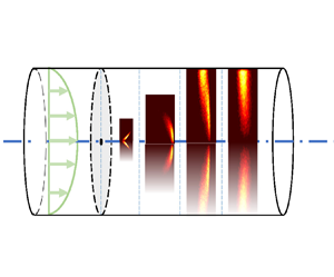
Figure 1. Illustration of transient Taylor dispersion for a central point release in a Poiseuille tube flow. Note that the illustrated concentration distribution is averaged azimuthally.

As practised widely in continuum mechanics (Crank Reference Crank1975; Hahn & Özişik Reference Hahn and Özişik2012), a convected coordinate system that moves with the fluid particle along each streamline is introduced,

(3.7)\begin{equation} {x}=\xi-{\textit{Pe}}\,u(r)\,t, \end{equation}

for a convection transformation to decouple convection from the diffusion effect. A Poiseuille tube flow velocity hereafter should be substituted as $u(r) =1-r^{ 2}$. Notice that as an original case in scalar transport, an upwind transformation has been devised for the construction of compact finite difference schemes for the convective–diffusion equation by Chen & Gao (Reference Chen and Gao1991) and Chen, Gao & Yang (Reference Chen, Gao and Yang1993). Substituting this transformation (3.7) into the normalised convection–diffusion equation with the chain rule yields a diffusion equation

(3.8)\begin{equation} \frac{\partial C}{\partial t}=\boldsymbol{\nabla}\boldsymbol{\cdot} (\boldsymbol{\mathsf{D}}\,\boldsymbol{\nabla} C), \end{equation}

with the divergence operator

(3.9)\begin{equation} {\boldsymbol{\nabla}\boldsymbol{\cdot} \boldsymbol{g}}=\frac{\partial g_x}{\partial {x}} +\frac{1}{r}\,\frac{\partial (rg_r)}{\partial {r}}, \end{equation}

where $g_x$ and $g_r$ are the axial and radial components of $\boldsymbol {g}$, respectively. This diffusion-type formulation can be obtained from a first principle with reference to figure 2.

Figure 2. Convection–diffusion analysis in the ordinary cylindrical coordinates $(\xi,r,\theta )$ and differential control volume $\mathrm {d}\kern 0.06em x \times r \,\mathrm {d}\theta \times \mathrm {d}r$, in the form of a pure diffusion equation for the convected system $(x,r,\theta )$.

The rate of transfer of diffusing matter through unit area of a cross-section is given by Fick's law as

(3.10)\begin{equation} \boldsymbol{j}={-}\boldsymbol{\nabla} C, \end{equation}

where the gradient operator is

(3.11)\begin{equation} {\boldsymbol{\nabla} f(x,r)} \equiv \left[\begin{matrix} \dfrac{\partial f(x,r)}{\partial {x}} \\ \dfrac{\partial f(x,r)}{\partial {r}} \end{matrix}\right], \end{equation}

and using the chain rule, the concentration flux components in the axial and radial directions are, respectively,

(3.12a,b)\begin{equation} j_{x}={-}\frac{\partial C}{\partial x},\quad j_{r}={-} \left(2\,{\textit{Pe}}\,t r\,\frac{\partial C}{\partial x} +\frac{\partial C}{\partial r}\right). \end{equation}

In the convected coordinate system, we now calculate each component normal to the section of the differential control volume. The rate of increase of dispersing matter through the inward section is given by

(3.13)\begin{equation} r\,\mathrm{d}\theta\left( j_{r}-\frac{1}{2}\,\frac{\partial j_{r}}{\partial r}\, \mathrm{d}r \,\mathrm{d}x-{\textit{Pe}}\,t r\,\frac{\partial j_{r}}{\partial x}\, \mathrm{d}x \,\mathrm{d}r\right), \end{equation}

and the rate of loss through the outward section is

(3.14)\begin{equation} r\,\mathrm{d}\theta\left(j_{r}+\frac{1}{2}\,\frac{\partial j_{r}}{\partial r}\,\mathrm{d}r \,\mathrm{d}x +{\textit{Pe}}\,t r\,\frac{\partial j_{r}}{\partial x}\,\mathrm{d}x\,\mathrm{d}r\right). \end{equation}

Thus the total contribution to the rate of increase of dispersing matter in the element between these two faces is equal to

(3.15)\begin{equation} -\! r\,\mathrm{d}\theta \,\mathrm{d}x\, \frac{\partial j_{r}}{\partial r}\,\mathrm{d}r-2\,{\textit{Pe}}\,t r^{ 2}\,\mathrm{d}\theta \,\mathrm{d}r\, \frac{\partial j_{r}}{\partial x}\,\mathrm{d}x. \end{equation}

Similarly, for the longitudinal faces we obtain

(3.16)\begin{equation} -\! r\,\mathrm{d}\theta \,\mathrm{d}r\, \frac{\partial j_{x}}{\partial x}\,\mathrm{d}x. \end{equation}

Note that the rate of change of dispersing matter in the control volume is

(3.17)\begin{equation} r\,\mathrm{d}\theta \,\mathrm{d}x \,\mathrm{d}r\,\frac{\partial C}{\partial t}. \end{equation}

Combining the above contributions, the conservation law requires for the axisymmetrical case

(3.18)\begin{equation} \frac{\partial C}{\partial t}+ \frac{\partial j_{r}}{\partial r} +2\,{\textit{Pe}}\,t r\,\frac{\partial j_{r}}{\partial x}+ \frac{\partial j_{x}}{\partial x}= 0. \end{equation}

Then the substitution of (3.12a,b) into (3.18) results in (3.8). Accordingly, the equivalent diffusivity tensor in (3.8) is obtained as

(3.19)\begin{equation} {\boldsymbol{\mathsf{D}}}=\left[\begin{matrix} 1+{{ ({{\textit{Pe}}\,{t}})}^{2}}\,{{|{\nabla}u|}^{2}} & -{\textit{Pe}}\,{t}\,{ {\boldsymbol{\nabla}}u} \\ -{\textit{Pe}}\,{t}\,{ {\boldsymbol{\nabla}}u} & 1 \end{matrix}\right].\end{equation}

The convection transformation deduces naturally three time scales with respect to the product of the Péclet number and dimensionless time, with a partition of $\boldsymbol{\mathsf{D}}$

(3.20)\begin{equation} \boldsymbol{\mathsf{D}}={\boldsymbol{\mathsf{D}}^{(\boldsymbol{\mathsf{O}})}}+ {{\textit{Pe}}\,{t}}{\boldsymbol{\mathsf{D}}^{(\boldsymbol{\mathsf{C}})}}+ {{({{\textit{Pe}}\,{ t}})}^{2}}{\boldsymbol{\mathsf{D}}^{(\boldsymbol{\mathsf{E}})}}, \end{equation}

wherein

(3.21a–c)\begin{equation} {\boldsymbol{\mathsf{D}}^{(\boldsymbol{\mathsf{O}})}}=\left[\begin{matrix} 1 & 0 \\ 0 & 1 \end{matrix}\right],\quad {\boldsymbol{\mathsf{D}}^{(\boldsymbol{\mathsf{C}})}}=\left[\begin{matrix} 0 & {\boldsymbol{\nabla}}u \\ {\boldsymbol{\nabla}}u & 0 \end{matrix}\right],\quad {\boldsymbol{\mathsf{D}}^{(\boldsymbol{\mathsf{E}})}}=\left[ \begin{matrix} {{| {\nabla}u|}^{2}} & 0 \\ 0 & 0 \end{matrix}\right].\end{equation}

The first tensor ${\boldsymbol{\mathsf{D}}^{(\boldsymbol{\mathsf{O}})}}$ represents the isotropic molecular diffusion of soluble matter; the second tensor ${\boldsymbol{\mathsf{D}}^{(\boldsymbol{\mathsf{C}})}}$ denotes a cross-enhancement due to the velocity shear; and the third tensor ${\boldsymbol{\mathsf{D}}^{(\boldsymbol{\mathsf{E}})}}$ quantifies a dispersal enhancement along the axial direction. With the decomposition, (3.8) is detailed as

(3.22)\begin{equation} \frac{\partial {{C }}}{\partial {t}}={\boldsymbol{\nabla}} \boldsymbol{\cdot} ({\boldsymbol{\mathsf{D}}^{(\boldsymbol{\mathsf{O}})}}\,{\boldsymbol{\nabla}}{{C }})+ {\textit{Pe}}\,{t}\,{\boldsymbol{\nabla}}\boldsymbol{\cdot} ({\boldsymbol{\mathsf{D}}^{(\boldsymbol{\mathsf{C}})}}\,{\boldsymbol{\nabla}}{C})+ {{({\textit{Pe}}\,{t})}^{2}}\,{\boldsymbol{\nabla}}\boldsymbol{\cdot} ({\boldsymbol{\mathsf{D}}^{(\boldsymbol{\mathsf{E}})}}\,{\boldsymbol{\nabla}}{C}). \end{equation}

For a given Péclet number, at a short time we retain a conventional isotropic diffusion equation,

(3.23)\begin{equation} \frac{\partial {{C }}}{\partial {t}}=\frac{\partial^2 {{C }}}{\partial {{x}^{2 }}} +\frac{1}{r}\,\frac{\partial {} }{\partial {r}} \left( r\,\frac{\partial {C} }{\partial {r}} \right), \end{equation}

and for long times, we obtain a one-dimensional streamwise diffusion equation,

(3.24)\begin{equation} \frac{\partial {{C }}}{\partial {t}}=4 r^{ 2}\,{\textit{Pe}}^2\,t^{2}\,\frac{\partial^2 {{C }}}{\partial {{x}^{2 }}}, \end{equation}

corresponding to the one-dimensional longitudinal diffusion equation for the transverse mean concentration in Taylor's overall dispersion model.

3.2. Taylor's dispersion model and its extensions

A solution of Taylor's form for asymptotically long time can be inferred promptly from (3.24). Before deriving a short-time particular solution with the streamwise theory of transient dispersion, we would like to first explain the nature of the model solution by Taylor (Reference Taylor1953) and some theoretical generalisations since then.

Consistent with Taylor (Reference Taylor1953), Aris (Reference Aris1956), Chatwin (Reference Chatwin1970) and Gill (Reference Gill1971), we introduce a longitudinal coordinate $x^\prime =\xi -{\textit{Pe}}\,\bar {U} t$ at the speed of mean flow velocity $\bar {U} \equiv \int _{0}^{1} u(r)\,2r \,{\rm d} r$, for comparison with the classical theoretical results. In all figures hereafter, a normalised set of $(\bar {C}\,{\textit{Pe}},x^\prime /{\textit{Pe}})$ is adopted. In Taylor's fashion, the convection–diffusion problem can be characterised by a one-dimensional enhanced diffusion equation of mean concentration $\bar {C} \equiv \int _{0}^{1} {C}\, 2r\,\mathrm {d}r$, well known as the Taylor dispersion model, as

(3.25)\begin{equation} \frac{\partial \bar{C}}{\partial t}= K_2\,\frac{\partial ^2 \bar{C}}{\partial x^{\prime 2}}. \end{equation}

To determine the coefficient of diffusion $K_2$, Taylor (Reference Taylor1954a) assumed that the concentration can be obtained with a Taylor expansion in the vicinity of mean concentration as

(3.26)\begin{equation} C=\bar{C}+\sum_{n=1}^{2} {K_n(r)\,\frac{\partial^n \bar{C}}{\partial x^{\prime n}}}. \end{equation}

By finding a general solution for the radial diffusion equation, he determined $K_1$. The second-order concentration gradient can be regarded as a small variation in $\partial C / \partial x^\prime$. Substitution of (3.26) into a reduced convection–diffusion equation yields $K_2$. By analogy with Taylor's manipulation, Gill proposed the transient dispersion model (Gill Reference Gill1967, communicated by Taylor), as

(3.27)\begin{equation} C=\bar{C}+\sum_{n=1}^{\infty} {f_n(t,r)\,\frac{\partial^n \bar{C}}{\partial x^{\prime n}}}, \end{equation}

which includes Taylor's model as a special case. Jiang & Chen (Reference Jiang and Chen2018) solved Gill's transient dispersion model by a systematic analytical procedure. The most effective and prevalent approach to solving the macro-scale equation is expressed in the form of a Kramers–Moyal expansion, i.e. an infinite series of spatial derivatives of concentration. Several successful attempts have been carried out by Chatwin (Reference Chatwin1970), Gill (Reference Gill1971), Smith (Reference Smith1982b) and others.

Inspired by (3.22), it is time to reflect on the extensions of Taylor dispersion and generalise the implications to transient dispersion. Taylor (Reference Taylor1953) assumed that the dispersion of a solute relative to the coordinate system moving with the mean flow speed could be predicted by an effective one-dimensional diffusion equation. From a first principle, we show by a convection transformation with the streamwise speed of flow in contrast to Taylor (Reference Taylor1954a): ‘the combined effect of longitudinal convection and radial molecular diffusion is to give rise to a transfer across planes which move with the mean speed of flow’, which ‘would only be likely to be valid when the time necessary for a radial variation in concentration to die down owing to radial diffusion was much shorter than the time necessary for an appreciable change in concentration to occur through longitudinal convection’. Furthermore, it is clear from (3.22) that the dispersion driven by convection and diffusion is indeed a diffusion process without arbitrary assumptions as perceived from a streamwise convected coordinate system. A partition of the equivalent diffusivity tensor, with respect to three time scales, shows that the components are anisotropic in space and nonlinear with time. The anisotropy and nonlinearity that complicate the dispersion process are due to the cross-shear effect and axial dispersal enhancement from a convected coordinate. As a result, Gaussian approximations are broadly pursued to reproduce the exact transient dispersion, although no conceptual conclusion has been reached on the matter.

3.3. Short-time particular solution

For an instantaneous release as symbolised by an axisymmetrical Dirac delta function for the initial concentration distribution, at small times the solution for (3.23) promptly reads

(3.28)\begin{equation} {C}=\frac{2{\rm \pi}}{{{ 16 {\rm \pi}^{3/2} {{t}^{ 3/2}} }}}\exp \left\{-\frac{{{[\xi- {\textit{Pe}}\,( 1-{{r}^{2}}){t}]}^{2}} +{{(r-r_0)}^{2}}}{4{t}}\right\} \end{equation}

for a source released at $\xi =0$, $r=r_0$ in a distance away from the wall. Note that for a small time, there is actually no effect of the boundary wall for an initial central point release of soluble matter, so that the solute disperses as if it were in infinite space from a convected perspective. This short-time particular solution (3.28) applies to instants just after the discharge and implies that the concentration distribution asymptotes to a tilted Gaussian form viewing from each fluid particle. In the Eulerian description moving at the mean flow speed, a long-tailed distribution should be predicted rather than the normal distribution as predicted by Saffman (Reference Saffman1960) and Smith (Reference Smith1982b). Therefore, our fundamental source solution derived for the initial stage is essentially different from previous well-established approximations. The solutions of initial axial Gaussian type sources, area sources and other non-uniform sources (e.g. initial conditions adopted in Abbott et al. Reference Abbott, Denman, Powell, Richerson, Richards and Goldman1984; Gekle Reference Gekle2017; Taghizadeh et al. Reference Taghizadeh, Valdés-Parada and Wood2020) can also be obtained with the superposition of the Green function from the solution of point sources directly, though the solutions from the Gaussian sources or area sources obtained in this manner would be physically meaningless without accounting for the interactions between soluble matter and the boundary. This solution works exactly at very short times when the majority of a solute has not approached the wall, in contrast to Saffman's approximation, which is true only for sufficiently small distance away from the centre in an infinite medium. The solution of Lighthill (Reference Lighthill1966) simply takes the conventional assumption in the dispersion analysis that the longitudinal diffusion can be neglected as compared to the convection effect. This condition is not realistic and even contrary to the inherent characteristics of the very initial phase when longitudinal diffusion can be dominant over convection upon instantaneous release of the source. Complexity in his solution results from this non-physical assumption, which is indeed valid for the anomalous regime (Chatwin Reference Chatwin1976) rather than the initial stage as declared. In contrast, the straightforward procedure presented in this section indicates the accuracy of (3.28) as a particular solution with physically reasonable approximations, and gives us conceptual insights that the dispersing solute in unsteady parallel flows is actually subject to the equivalent diffusion equations viewed from a convected coordinate system, corresponding to three scales specified by a product of the Péclet number and diffusive time.

For larger times in the initial phase when the solute cloud may appear in the zone near the wall, the boundary restrictions can be released to a first-order approximation by the method of image. When an imaged source is introduced to make the resulting concentration symmetric about the tangent of the tube boundary, the radial derivative of concentration becomes zero, exactly as required by the boundary conditions. From the reduced governing equation (3.1), the axial symmetry and uniqueness of the unit source solution guarantee the effectiveness of the image method as if it were applied to an infinite plane. An image method is applied to account for the reflective boundary condition as

(3.29)\begin{align} {{C }} &= \frac{2{\rm \pi}}{{{16 {\rm \pi}^{3/2} {{t}^{ 3/2}} }}}\exp \left\{-\frac{{{[\xi- {\textit{Pe}}\,(1-{{r}^{ 2}}){t}]}^{2}}+{{(r-{{r}_{0}})}^{2}}}{4{t}} \right\} \nonumber\\ &\quad +\frac{2{\rm \pi}}{{{ 16 {\rm \pi}^{3/2} {{t}^{ 3/2}} }}} \exp \left\{-\frac{{{[\xi-{\textit{Pe}}\,(1-{{({r}-2+{{r}_{0}})}^{2}}){t}]}^{2}}+ {{({r}-2+{{r}_{0}})}^{2}}}{4{t}} \right\}. \end{align}

Interestingly, the unified short-time solution (3.29) shows wide adaptability up to $t \sim 0.1$, as shown in figure 3(d), compared with Monte Carlo simulation results for characteristic dispersion regimes, where numerical procedures are detailed in § 1 of the supplementary material available at https://doi.org/10.1017/jfm.2024.34. This time scale characterises the initial dispersion regime, almost reaching the lower bound of the applicable time limit of existing extended dispersion models.

Figure 3. Mean concentration distribution in a Poiseuille tube flow predicted by the short-time particular solution (3.29) compared with the Monte Carlo simulation at times (a) $t=1.0 \times 10^{-4}$, (b) $t=1.0 \times 10^{-2}$, (c) $t=5.0 \times 10^{-2}$, and (d) $t=1.0 \times 10^{-1}$, in Taylor's moving coordinate system. Common parameters are ${\textit{Pe}}=10\,000$ and $r_0=0$.

The distinctive characteristics of the initial regime are symmetric Gaussian profiles when molecular diffusion is predominant over axial convection, as shown in figure 3(a). Physically, the convection transformation represents a streamwise perspective viewing from fluid particles. In such a convected coordinate system, a solute experiences pure diffusion within the initial stage, axially and radially, in a highly symmetric manner similar to the Taylor regime. When the velocity shear dominates axial diffusion, unidirectional convective distortion of the flow field breaks the symmetry and flushes the peaks of mean concentration distribution downstream within the anomalous regime. The head and tail of the concentration profiles are unique features for the transient dispersion, as shown in figures 3(b–d). Latini & Bernoff (Reference Latini and Bernoff2001) deduced head and tail approximations for this stage, describing the distortion of the mean concentration profile, respectively. In contrast, the present particular solution gives a compact and precise description of this highly skewed shape of the distribution with lesser substantial error. On the whole, the short-time particular solution (3.29) gives satisfactorily quantitative predictions and reveals new physical structures, complementary to Taylor's long-time solution.

4.1. Implications of physical structures from diffusion flux vectors

To better understand the implications of the physical structures, we resort to the diffusion flux vector in the convected coordinate system as

(4.1)\begin{equation} \boldsymbol{j}=\left[\begin{array}{c} -(1+4\,{\textit{Pe}}^2\,t^{2}r^{2})\,\dfrac{\partial C}{\partial x}-2\,{\textit{Pe}}\,t r\,\dfrac{\partial C}{\partial r} \\ -\dfrac{\partial C}{\partial r}-2\,{\textit{Pe}}\,t r\,\dfrac{\partial C}{\partial x} \end{array}\right]. \end{equation}

This expression lends the ground for two observations. The first is that the diffusion in the axial direction is enhanced by the velocity shear, with the extent of enhancement quantified by $4\,{\textit{Pe}}^2\,t^{2}r^{2}$. This axial enhancement due to the shear is represented by ${\boldsymbol{\mathsf{D}}^{(\boldsymbol{\mathsf{E}})}}$. Second, the diffusion in the axial direction is translated into the radial gradient flux with the extent of enhancement quantified by $2\,{\textit{Pe}}\,t r$. This cross-shear enhancement is represented by ${\boldsymbol{\mathsf{D}}^{(\boldsymbol{\mathsf{C}})}}$.

The vector (4.1) is heuristic to analyse the original convection–diffusion equation from a Lagrangian view. Enhanced effects are directly proportional to the magnitude of the velocity gradient, and the duration of dispersion also positively correlates with the enhanced effects. The shear varies throughout the flow domain, and these effects are anisotropic and inhomogeneous in the prescribed flow domain at different times. Further, there must be a predefined sub-region for a solute to demonstrate a preference for release positions, leading to an expedited dispersion process, provided that the velocity profile and observation time remain unchanged.

Based on the above analysis, we exemplify a circular ribbon of a solute in a classical Poiseuille tube flow, given that the ribbon is thin in the radial direction and narrow in the axial direction, being released exactly near the tube wall ($r_0 \sim 1$) at $t=0$. The Eulerian non-penetration boundary condition at the wall ($\partial C / \partial r=0$) in the convected coordinate becomes a no-flux condition ($\partial C / \partial r +2\,{\textit{Pe}}\,t r\,\partial C / \partial x =0$) at $r=1$.

The intrinsic feature of Poiseuille tube flow determines that $|\boldsymbol {\nabla } u|$ is largest at the wall. Remarkable cross and enhanced shear effects are exerted on the circular ribbon. Hereafter, we analyse the interaction with the tube wall by (4.1). It implies that the diffusion along the streamwise direction is enhanced, and the solution will disperse from its two ends along the tube wall in both the positive and negative directions of $x$. At the front end of the ribbon, $\partial C / \partial x<0$. Therefore, we have the cross-effect $-2\,{\textit{Pe}}\,t r\,\partial C / \partial x >0$. With the aid of the zero-flux condition in the radial direction, we deduce that $\partial C / \partial r>0$ at $r=1$. Physically, the shear effect tends to make the solution disperse in the positive radial direction towards the wall. Likewise, for the rear end of the ribbon, the cross-effect makes the solution disperse towards lower $r$.

We then focus on convection due to horizontal gradients and lateral diffusion. On the inner surface of the ribbon, $\partial C / \partial r>0$. With the aid of the zero-flux condition in the radial direction, we deduce that $2\,{\textit{Pe}}\,t r\,\partial C / \partial x<0$ and thus $\partial C / \partial x<0$. Physically, the enhanced effect tends to make the solution disperse towards the negative direction of $x$. Convection occurs because horizontal variations in concentration are produced by the radial diffusion. Similarly, for the outer surface contacting the wall, we can indicate that the enhanced effect tends to disperse the solution towards positive $x$.

The foregoing analysis gives a picture of how the ribbon is distorted in a tube flow. To illustrate the shear effect and interaction with the wall boundary, we further explore how the asymmetries are caused by diffusion and interaction with the tube wall. As shown in figure 4, the initial concentration distribution of the ribbon is uniform. Due to the shear enhancement, the ribbon's shape would be distorted. Relative to the front part, the rear of the ribbon tends to spread radially more towards the tube axis, and then the inner solution tends to disperse axially more towards the negative direction. Caused by the interaction with the wall, the solute retaining near the wall disperses inwards and backwards. Hence the rectangular shape of mean concentration by the pure convection evolves gradually into a skewed platform, with an asymmetric peak in the rear part, as shown in figure 4. The manifestation of this asymmetry has emerged frequently in the development of both area and point sources. For instance, the initial area source and convection-induced rectangles both experience this kind of symmetry breaking. For the case of a uniform discharge, Chatwin (Reference Chatwin1970) interpreted the evolution with his physical intuition. The interpretation could be extended on a rigorous basis of mathematical formulae for wider initial sources. The strength of our derivation (3.29) lies in its compactness and simplicity with the combination of precision in quantity. As illustrated in figure 3, it also outweighs as an analytical particular solution from the very initial release towards the transitional stage.

Figure 4. Physical interpretation of the uniform distribution to the asymmetric platform caused by the shear effect and interaction with the wall. The filled graph is computed by full numerical solutions of the convection–diffusion equation (CDE), and the cyan line is predicted by the pure advection model as a uniform distribution from an area source at $t=0.15$.

4.2. Persistence of asymmetries and their origins

With the understanding that a direct Gaussian approximation could not reproduce the multi-peaked structure (Smith Reference Smith1982b), efforts directly from the solution of Saffman or Taylor should contribute little in effect to feature the ‘skewed platform’ in figure 4. Since the asymmetries could be persistent, it is of research interest to investigate the following questions. (i) What are the origins of the symmetry breaking of mean concentration distribution? (ii) What physical patterns could emerge during the convection–diffusion process, as time elapses from $0$ to $\infty$?

First, the initial distribution could be inhomogeneous in its own right. This initial non-uniformity of the soluble matter could be rather persistent before reaching the Taylor dispersion regime. In terms of moments and cumulants, the skewness may deviate from zero initially, thus mean concentration could be asymmetric. Hence an origin of asymmetries along the axial direction is present soon whether or not the ribbon is distributed uniformly initially.

Second, the unidirectional convective distortion plays an important role in symmetry breaking. For instance, the cloud of soluble matter could have a long-tailed distribution as shown in figure 5, stretched either upstream or downstream. This remarkable feature is first captured qualitatively by a pure advection model of Taylor (Reference Taylor1953) from a point moving at the mean speed of the flow.

Figure 5. Physical interpretation of the long-tailed distribution to the asymmetric platform caused by the shear effect and interaction with the wall. The filled graph is computed by full numerical solutions of the convection–diffusion equation (CDE), and the cyan line is predicted by (3.29) from a central point source at $t=0.2$.

Third, the zero-flux effect of the wall boundary serves as another origin of asymmetries. The zero-gradient boundary condition at the wall ($\partial C / \partial r=0$), in the convected coordinate becomes a zero diffusion flux condition ($\partial C / \partial r +2\,{\textit{Pe}}\,t r\,\partial C / \partial x =0$) at $r=1$. The interaction with the wall gives rise to typically skewed platforms, which are highly unsymmetrical. We confirm in figure 5 that the asymmetry can be caused by only diffusion and interaction with the wall.

In summary, we certify theoretically that the asymmetries of concentration distribution through a circular tube have at least three origins, basically: (a) initial non-uniformity, (b) unidirectional convective distortion, and (c) zero-flux effect of wall boundary.

In figures 4 and 5, the pure advection solution and short-time diffusion solution are illustrated to show the origins of the asymmetric physical patterns, which still deviate from the convection–diffusion equation for specific times during the transitional stage. The mismatch is obviously due to the cross-effect, i.e. the second term on the right-hand side of (3.22), and low-order image approximations of the boundary effect, which precludes the soluble matter from being rotated and elongated into a more skewed and smooth profile. Likewise, the enhanced diffusion effect, i.e. the third term on the right-hand side of (3.22), would shape the rectangular profile into a symmetric Gaussian form.

Before approaching the second problem, we would like to exemplify the transient dispersion from a point source to illustrate the symmetry breaking during the temporal evolution of concentration distributions. The fundamental case gives a comprehensive picture of how the diffusion process translates from one pattern to another as time elapses. For the transient dispersion of a solute discharged from a point source on the axis, there are virtually four dispersion regimes developing incrementally, say a longitudinal diffusive regime, two transitional (anomalous diffusion and pre-asymptotic) regimes, and a Taylor dispersion regime from an initially short time to asymptotically long times. With the Monte Carlo simulation, we illustrate the four dispersion regimes with corresponding transverse and mean concentration distributions as presented in figure 6. For short times, the longitudinal diffusion is predominant over either convection or radial diffusion. Provided that a blob of point sources is injected into the lateral position far from the wall, the solute cloud will diffuse isotropically, in the convected coordinate system. In other words, the spread of the point source follows a modified Gaussian distribution initially as shown in figure 6(c). The anomalous diffusion regime is an intermediate stage where complicated balance mechanisms occur. The widely recognised pure convection model is applicable to this stage, as is Lighthill's exact solution (Lighthill Reference Lighthill1966). However, it should be noted that Lighthill's solution imposed impractical limitations, potentially rendering the predictions inconsistent with the physical manifestation of the natural dispersion process. In fact, the mean concentration distribution should exhibit a rectangular shape as predicted neither by the pure advection model due to the neglect of lateral diffusion, nor by Lighthill's modified approximation due to the neglect of wall effect. Lighthill's exact solution serves as an interaction mechanism within the anomalous diffusion regime, distinct from the initial stage. Subsequently, this facilitates the examination of lateral diffusion influenced by boundary walls and convection. Consequently, there exist two balance mechanisms before and after the unachievable pure advection stage. The former is influenced predominantly by longitudinal diffusion and advection, while the latter is affected primarily by advection and lateral diffusion. The interaction between tube walls and particles in the presence of external hydrodynamic conditions leads to the emergence of symmetry breaking and multi-scale characteristics, which align with the transition between these two mechanisms. Technically, it remains most difficult to account for this transition from the anomalous diffusion stage to the pre-asymptotic regime, shown in figures 6(d,g). For asymptotically long times, Taylor (Reference Taylor1953) described the enhanced longitudinal dispersion under the combined action of advection and lateral diffusion. In particular, the longitudinal normality ($t \gtrsim 1$; Chatwin Reference Chatwin1970) and transverse uniformity ($t \gtrsim 10$; Wu & Chen Reference Wu and Chen2014) have been explored systematically, as shown in figure 6(h).

Figure 6. Four dispersion regimes in the transient dispersion (after figure 2 on p. 402 of Latini & Bernoff Reference Latini and Bernoff2001). The azimuthally averaged concentration distributions of a solute in the tube with rotational symmetry are calculated with the Monte Carlo simulation, with the two-dimensional concentration contours and mean concentration $\bar {C}$ line graphs plotted as functions of the longitudinal axis $x$ and/or radial axis $r$. (a,c) The longitudinal diffusive regime at $t=1.0 \times 10^{-4}$. (b,d) The anomalous diffusion regime at $t=1.0 \times 10^{-2}$. (e,g) The pre-asymptotic regime at $t=2.0 \times 10^{-1}$. (f,h) The Taylor dispersion regime at $t=1.0$. Common parameters are ${\textit{Pe}}=10\,000$ and $r_0=0$.

5.1. Streamwise dispersion model in local moment space

To further investigate the second question posed in § 4.2, we revisit the convectively transformed governing equation (3.22). The equivalent transformed equation indicates a superposition of three effective diffusion processes. The second concern then transforms into how the effective diffusion processes take turns to dominate. From (3.28), which applies to short times after a discharge from the initial point source, the concentration distribution asymptotes to a modified Gaussian form. For longer times, the cross-shear effect – i.e. the second term on the right-hand side of the convectively transformed governing equation – is predominant to introduce asymmetries. When the solute cloud approaches the wall, the interaction with the wall will further lead to symmetry breaking. For asymptotically long times, the enhanced streamwise diffusion term along the axial direction – i.e. the third term on the right-hand side of the convectively transformed governing equation – dominates other contributions. This paves the way naturally to the Taylor dispersion model, i.e. the convection–diffusion process is characteristic of one-dimensional enhanced diffusion for asymptotically long times. Taylor (Reference Taylor1953) made an assumption that the effective diffusivity is independent of time or space. Based on a Taylor expansion of concentration distribution at the vicinity of mean concentration, the dispersivity can be derived by inversion. Note that the formal convection–diffusion process belongs intrinsically to diffusion type from the perspective of the moving fluid particles, whilst the effective diffusivity should vary nonlinearly with time and anisotropically in space.

The limitation of (3.22) for analytical approaches is that nonlinear terms make it hard to be mathematically tractable. However, we emphasise that the general convection transformation and short-time particular solution reveal novel physical structures of transient dispersion. From the implications of the convectively transformed equation, an exact diffusion-type description is formulated. We can make use of the exact solutions of local concentration moments to determine the nonlinear diffusion coefficients. We will formulate a streamwise expansion matching the convection transformation in local moment space, with the aim of reproducing accurately the featured physical structures.

Upon utilising a convection transformation, the short-time particular solution of concentration of pointwise soluble matter follows a modified Gaussian distribution viewing from the fluid particles. The short-time particular solution of the convection–diffusion equation is derived from the perspective of fluid particles valid for times before most soluble matter approaches the boundary wall, complementary to the Taylor dispersion model. It is predicted and verified that a tilted Gaussian distribution of concentration appears long before a paraboloidal snout has been pulled out by the Poiseuille tube flow, which later skews when colliding with the wall, and eventually disperses into an equilibrium Taylor dispersion state. On the other hand, the long-time convectively transformed equation also implies an asymptotic dispersion solution of point discharge in a bounded flow, corresponding to a typical Gaussian distribution as suggested originally by Taylor (Reference Taylor1953).

The basic mechanism of Taylor dispersion is general in both cases, even though Gaussian approximation may fail in the transition stage. A significant advance of Smith (Reference Smith1982b) for a Gaussian approximation along the streamline with a uniform area source stems from the short-time approximated source solution of Saffman (Reference Saffman1960) and the long-time Gaussian solution of the Taylor dispersion model. He was disappointed that a direct Gaussian approximation could not reproduce the asymmetric characteristics and later designed a delay–diffusion model (Smith Reference Smith1981, Reference Smith1982a). Aimed at the inaccuracy of the Gaussian approximation of Smith (Reference Smith1982b) for asymptotically short times, Li (Reference Li2018) extended the Taylor–Aris method for the transverse concentration in the spirit of streamwise dispersion. This second-order Taylor–Aris description could not only depict well the early stage whence the transport of the solute is governed by longitudinal diffusion and convection, but also recover the long-time evolution of dispersion without resorting to higher-order terms. The basic asymmetric physical structure is produced qualitatively for the first time as a breakthrough. However, the quantitatively satisfactory reproduction of asymmetric physical structures, especially during the pre-asymptotic regime, still remains desirable yet elusive to date. A streamwise expansion from the asymptotic analysis shows that the concentration distribution is subject to a modified Gaussian distribution in local moment space. By taking into account the Edgeworth modification in statistical theory, a streamwise dispersion model would be devised to fill in this gap.

A streamwise coordinate, which moves initially at the local velocity of the external flow field and eventually at the mean flow speed, naturally comes from these two limits, as will be normalised later, in (5.6). Define the marginal probability density function $P$ as

(5.1)\begin{equation} P(\xi,r,t\,|\, \xi_0, r_0 )=\frac{C(\xi,r,t)}{\displaystyle\int_{-\infty}^{\infty}C(\xi,r,t) \,\mathrm{d}\xi}, \end{equation}

which gives the probability of the tracer present at the point $(\xi, r)$ at time $t$, given its initial release at the point $(\xi _0, r_0)$. The Fourier transform of the probability density function gives the cumulant-generating function with respect to the angular frequency $k$ as

(5.2)\begin{equation} \phi(k,r,t)\equiv \int_{-\infty}^{\infty} P \exp ({\rm i} k \xi) \,\mathrm{d} \xi. \end{equation}

This cumulant-generating function could be obtained with the natural logarithm (Kendall & Stuart Reference Kendall and Stuart1958; Chatwin Reference Chatwin1970; Jiang & Chen Reference Jiang and Chen2018) as

(5.3)\begin{equation} \ln \phi =\sum_{n=1}^{\infty }{\kappa_n}\,\frac{(\mathrm{i}k)^n}{n!}, \end{equation}

wherein $\kappa _n$ is the $n$th-order cumulant, which could be obtained directly through central moments, as is computed in the supplementary material. Substitution of (5.3) into the inverse transform of $\phi$ gives

(5.4)\begin{equation} \frac{C(\xi, r, t)}{\displaystyle\int_{-\infty}^{\infty} C(\xi, r, t)\,\mathrm{d}\xi} =\frac{1}{2{\rm \pi}}\int_{-\infty}^{\infty} \exp\left[{\sum_{n=1}^{\infty }{\kappa_n}\, \frac{(\mathrm{i}k)^n}{n!}}\right] \exp (-{\rm i} k \xi) \,\mathrm{d} k.\end{equation}

Note that the denominator on the left-hand side is the zeroth moment. That is, the streamwise expansion inherently gives the relationship between concentration distribution and moments. Using the identity

(5.5)\begin{equation} \int_{-\infty}^{\infty} \exp \left(-{\rm i}k\xi-\frac{1}{2}\,k^2\right) ({\rm i} k)^n \,{\rm d} k=\sqrt{2 {\rm \pi}}\,{He}_{n}(\xi) \exp \left(-\frac{1}{2}\,\xi^2\right), \end{equation}

the Taylor expansion of the first exponential term on the right-hand side of (5.4), and Edgeworth's modification (Kendall & Stuart Reference Kendall and Stuart1958; Chatwin Reference Chatwin1970) embodied by square brackets, we could obtain a concise and accurate streamwise expansion with the normalised Eulerian coordinate as

(5.6)\begin{align} C(\xi,r,t) &= \frac{{C}_{0}}{\sqrt{2{\rm \pi} {{\kappa }_{2}}}}\exp \left[ -\frac{{{(\xi-{{\kappa }_{1}})}^{2}}}{{{\kappa }_{2}}} \right] \times \left\{1+\left[\frac{\kappa_3}{3! (\kappa_2)^{3/2}}\, {He}_{3} \left(\frac{{{ \xi-{{\kappa }_{1}} }}}{{{\kappa }_{2}^{1/2}}} \right)\right]\right. \nonumber\\ &\quad +\left.\left[\frac{\kappa_4}{4!\,\kappa_2^2}\,{He}_{4} \left( \frac{{{ \xi-{{\kappa }_{1}} }}}{{{\kappa }_{2}^{1/2}}} \right) + \frac{10\kappa_3}{6!\,\kappa_2^3}\,{He}_{6} \left(\frac{{{ \xi-{{\kappa }_{1}} }}}{{{\kappa }_{2}^{1/2}}} \right)\right]+\cdots\right\}, \end{align}

where $C_n(r,t) \equiv \int _{-\infty }^{\infty } C(\xi,r,t)\,\xi ^n \,\mathrm {d}\xi$ ($n=0,1,2,\ldots$) is the $n$th-order moment of concentration, and $\textit {He}_{n}$ is the Chebyshev–Hermite polynomial of $n$th order. Physically, $\kappa _1$ represents the advection velocity along each streamline, $\kappa _2$ is the streamwise mean square displacement applied to ensure unit variance for long times, $\kappa _3$ is the streamwise skewness quantifying the extent of asymmetry, and $\kappa _4$ is the streamwise kurtosis reflecting the sharpness of the peak. Note that this choice of streamwise coordinate well matches the spirit of streamwise theory in local moment space. While the basic term beyond the expansion is a unified expression for both the short- and long-time Gaussian distributions, the expansion in the bracket includes the Edgeworth modification. This well-known Edgeworth form of the Gram–Charlie series of type A in statistical theory is introduced in (5.6) to collect terms of the same order as manipulated in each square bracket and improve the convergence of the analytical model, as a reflection of transient effects.

Especially for the high-order terms, usual truncation methods would ignore corresponding contributions in the same order of magnitude with the assumption $\kappa _n = O (t^{1-n/2})$. Comparison of the present streamwise expansion with the original models of Chatwin (Reference Chatwin1970), Gill et al. (Reference Gill, Sankarasubramanian and Taylor1970) and Smith (Reference Smith1982b) will be made intensively in § 5.3 and § 5.4. The present streamwise expansion outweighs others for the current application of fundamental Dirac delta sources due to its accurate description of moments and superior astringency, whereas the generality of the streamwise dispersion theory is not affected. Significant improvement would be shown especially during the transitional regime before Taylor dispersion, in contrast to existing analytical models.

Streamwise dispersion of soluble matter subject to longitudinal advection and transverse diffusion is often described by an averaged dispersion coefficient over the cross-section. By extending further the Taylor dispersion theory, new definitions of this averaged amount for the effective diffusion coefficients in (5.11) should be adopted, however, to better capture the streamwise characteristics. In contrast to the coarse-grained Taylor–Aris dispersivity $\bar {D}_T$ defined as

(5.7)\begin{equation} \bar{D}_T= \frac{1}{2}\,\frac{\partial }{\partial t} [\bar{C}_2-(\bar{C}_1)^2], \end{equation}

Yasuda (Reference Yasuda1984) proposed a new averaging method

(5.8)\begin{equation} \bar{D}_T^S=\frac{1}{2}\,\frac{\partial }{\partial t} \left[\overline{\frac{{C}_2}{C_0}-\frac{{C_1^2}}{C_0^2}}\right], \end{equation}

where the overbar denotes a transverse averaging operator over the cross-section, to avoid the presence of negative streamwise dispersivity. The latter is denoted with a superscript $S$ to show its accuracy of streamwise information. Note that the asymptotic values yield to Taylor dispersivity $1+{\textit{Pe}}^2/48$ through a straight circular tube. Hereafter, we resort to these two definitions of transverse averaging of time-dependent effective diffusion coefficients, normalised by the asymptotic Taylor dispersivity, for better understanding of non-trivial and heuristic results of streamwise dispersion. The spatio-temporal evolution of time-dependent effective diffusion coefficients, commonly termed as transient dispersivity, is shown in figure 7, wherein the power of streamwise theory is revealed clearly. For long times, it is shown that the dispersion grows linearly with time, and dispersivity approaches transverse uniformity, whence the solute molecule has taken identical opportunity to sample the whole tube cross-section. This dispersion occurs due to the stochastic nature of radial Brownian diffusion; not all soluble matter discharged initially at $\xi =0$ will leave a fixed exit plane in the meantime. In other words, a distribution of transient dispersivity exists before the dispersion regime as displayed in figure 7(a).

Figure 7. Spatio-temporal evolution of time-dependent effective diffusion coefficients, normalised by the asymptotic Taylor–Aris limit ($\bar {D}_T({\infty })=1+{\textit{Pe}}^2/48$). (a) Transient streamwise dispersivity of (5.11) in a tube Poiseuille flow for ${\textit{Pe}}=10\,000$ with a central point source as a function of $r$ within different regimes. (b) Plot of the normalised streamwise dispersivity with $r_0=0,0.5,1$ and uniform area source. Peculiar characteristic peaks of transient dispersivity are revealed to exceed $\bar {D}_T({\infty })$ perceptibly. (c) Comparison of the coarse-grained Taylor–Aris dispersivity (5.7) and streamwise dispersivity (5.8) with ${\textit{Pe}}=10\,000$ and $r_0=0$. (d) The normalised streamwise dispersivity completely overlaps for different Péclet numbers, when streamwise variations in concentration due to advection remarkably outweigh molecular diffusion (${\textit{Pe}} \gg 1$).

Different initial conditions are adopted in figure 7(b), and the transient streamwise dispersivity about the mean uncovers a peculiar characteristic peak that perceptibly exceeds the Taylor–Aris limit ($1+{\textit{Pe}}^2/48$), which was reported through straight channels of arbitrary cross-section by Vedel et al. (Reference Vedel, Hovad and Bruus2014) for the first time. This interesting phenomenon is due to the delay of relaxation time between the first and second axial moments (Vedel et al. Reference Vedel, Hovad and Bruus2014). Only releases near the central axis could produce the unique peak in contrast to dispersion from uniform area and near-wall point sources or purely dissipative process like diffusion. Note that this non-monotonic variation of transient streamwise dispersivity corresponds to some particular dispersion regimes, from a fundamental level of probability density distribution. For example, the motion from a central point source is diffusive for the initial regime, then varies from super-diffusive to sub-diffusive during the anomalous regime, and eventually becomes diffusive once again within the dispersion regime. This peculiar characteristic peak of transient streamwise dispersivity could not only be mathematically understood from the deviation of first and second moments, but also physically explained as being a point from the classical continuum-mechanical perspective. The statistical trajectory of this locator point could represent the spreading of a solute through the flow. Released near the axis of the tube, the solute diffuses transversely from the centre to the wall before its approach to uniformity. The intrinsic convection of Poiseuille tube flow drives particles on the axis faster than those near the wall, leading to an enhanced axial spreading of the tracer in the presence of molecular diffusion compared to the fluid particle. This is responsible for the monotonic increase of streamwise dispersivity during the initial regime. Later, the effect of boundary sets in when the locator point diffuses radially outwards towards the wall, which results transiently in an asymmetric platform of concentration distribution and characteristic peak of streamwise dispersivity. The highly remarkable nonlinear contribution of Taylor dispersion with respect to molecular diffusivity from axial diffusion arises exactly from transverse molecular diffusion and axial convection. The smaller the molecular diffusivity, the more appreciable enhanced dispersion occurs. Before the locator solute behaves identically with the fluid particle in a kinematic sense in the long run, the transverse positions across the tube indeed do not attract the solute molecule equally. This preferential behaviour of the asymmetric transverse distribution is the key to the biases of drift velocities and streamwise dispersivities. Within the pre-asymptotic dispersion regime, the effect of flow convection and reflective wall indeed attenuate the transverse diffusion, and thus result in an enhanced axial spreading even exceeding the Taylor–Aris limit.

Comparison of the coarse-grained Taylor–Aris dispersivity and streamwise dispersivity is shown in figure 7(c). Although the peculiar peaks are shown for both definitions from a central point release, we emphasise that only the streamwise dispersivity exactly captures the axial displacement along each streamline, and clearly exhibits the remarkable enhancement of axial spreading. The overall Taylor–Aris dispersivity is instead a fictitious quantity of the whole cloud of soluble matter, which may exhibit negative values at small times; see e.g. Yasuda (Reference Yasuda1984, figures 8 and 10, p. 395), Guan et al. (Reference Guan, Zeng, Li, Guo, Wu and Wang2021, figure 13, p. 12) and Guan et al. (Reference Guan, Zeng, Jiang, Guo, Wang, Wu, Li and Chen2022, figures 11 and 12, pp. 14–15). As the crucial dimensionless parameter in this simple physical problem, the flow Péclet number quantifies the ratio of flow convection to molecular diffusion. In figure 7(d), we demonstrate that the normalised streamwise dispersivity completely overlaps with different Péclet numbers, when streamwise variations in concentration due to advection remarkably outweigh molecular diffusion. This limit is a requirement of Taylor dispersion, while its opposite limit could also be an interesting inverse problem outside the scope of this work. Although Péclet number influences significantly the absolute values of streamwise dispersivity, the normalised quantities presented in this paper are unified to illustrate the exact evolution.

It would be captivating to establish a link between these observations and the physical manifestations of transient dispersion, as depicted in figure 6, revealing four distinct dispersion stages within this problem. At the outset, dispersion results primarily from streamwise diffusion, prevailing over shear effects, as depicted in figure 6(a). For a central point source, the concentration distribution takes the form of a modified Gaussian, being convected by the streamwise flow velocity, as depicted in figure 6(c). During this stage, the streamwise dispersivity exhibits a zero slope, resembling ordinary isotropic diffusion, and is represented as a diffusive regime by Latini & Bernoff (Reference Latini and Bernoff2001).

The interplay of shear-induced convection with molecular diffusion gives rise to anomalous scaling, causing non-monotonic variations in streamwise dispersivity. Within this stage, in this work we have delineated two distinct regimes, depending on whether streamwise or lateral diffusion takes precedence. As shown in figures 6(d,g), the hallmarks of the above regimes are tilted Gaussian distributions and one skewed platform-like distribution, respectively. The transition initiates once the majority of soluble substances have traversed the streamlines to interact with the boundary. It is important to note that a distinctive peak, exceeding the Taylor–Aris limit, becomes evident as the non-penetration boundary effect comes into play during tracer dispersion. This corresponds to the right-skewed distribution of mean concentration, indicating a significantly enhanced solute dispersion in the pre-asymptotic transitional regime. The developed streamwise dispersion model has the capacity to capture these novel statistical and physical characteristics of mean concentration, including the distinctive heads and tails of the asymmetric concentration profiles.

Over time, in the Taylor dispersion regime, particles gradually approach transverse uniformity and streamwise normality, as illustrated in figures 6(f,h). The streamwise dispersivity once again demonstrates diffusive scaling, albeit in a notably enhanced fashion. Moreover, the concentration distribution reverts to a streamwise Gaussian distribution, corresponding to the longitudinal Gaussian distribution in Taylor's model.

5.2. Asymptotic analysis

The asymptotic behaviours of the concentration moment have been explored extensively. Following Aris (Reference Aris1956) and Li (Reference Li2018), we hereafter resort to the asymptotic analysis of the second-order streamwise model of transient dispersion, for both asymptotically short and long times. In this paper, the original coarse-grained Taylor–Aris drift velocity and dispersivity are denoted as $\bar {\varPhi }_T(t)$ and $\bar {D}_T(t)$, respectively. Viewing in a rather distinct perspective, we can transform the velocity and diffusion coefficients in Taylor's model to the drift velocity and dispersivity in their full-time dependence, and a second-order governing equation of streamwise expansion is obtained equivalently (Li Reference Li2018) as

(5.9)\begin{equation} \frac{\partial C (\xi,r,t )}{\partial t }+\varPhi^S_T\, \frac{\partial C (\xi ,r,t )}{\partial \xi }=D_T^S\, \frac{{{\partial }^{2}}C (\xi ,r ,t )}{\partial {{\xi }^{2}}}, \end{equation}

where the streamwise drift velocity is defined as

(5.10)\begin{equation} \varPhi^S_T \equiv \frac{\partial {\mu_1}}{\partial t }, \end{equation}

and time-dependent streamwise effective diffusion coefficients are defined as

(5.11)\begin{equation} D_T^S \equiv \frac{1}{2}\,\frac{\partial \mu_{2}} {\partial t}. \end{equation}

The central moment $\mu _n$ up to second order reads

(5.12a,b)\begin{equation} {{\mu }_{1}}(\xi,r,t)=\frac{{C}_{1}}{{C}_{0}},\quad {{\mu}_{2}}(\xi,r,t)=\frac{{{C}_{2}}}{{C}_{0}}-\frac{{C}_{1}^{2}}{{C}_{0}^{2}}. \end{equation}

The analytical solution of second-order streamwise dispersion theory could be derived as

(5.13)\begin{equation} C (\xi ,r, t )=\frac{{C}_{0}}{\sqrt{2{\rm \pi} ({{C}_{2}}/{C}_{0}-2C_{1}^{2}/{C}_{0}^{2})}}\exp \left[-\frac{{{(\xi -{C}_{1}/{C}_{0})}^{2}}}{2({{C}_{2}}/{C}_{0}-2 C_{1}^{2}/{C}_{0}^{2})}\right]. \end{equation}

For transient dispersion through a tube from a uniform area source, the first moment of a discharge for long times reads

(5.14)\begin{equation} C_{1}(r,t)={\textit{Pe}} \sum_{j=1}^{\infty} \frac{J_{0}(\theta_{j} r)}{J_{0}(\theta_{j})}\, \frac{\overline{J_{0}(\theta_{j} r)\,u}}{J_{0}(\theta_{j})}\, \frac{1-\exp({-t \theta_{j}^{2}})}{\theta_{j}^{2}}, \end{equation}

and the second moment is

(5.15)\begin{equation} C_{2}(r,t)=\bar{C}_{2}+2 t+2\,{\textit{Pe}}^{2} \sum_{j=1}^{\infty} \frac{\varphi_{j}^{2}}{\theta_{j}^{2}}\left[t-\frac{1-\exp({-t \theta_{j}^{2}})}{\theta_{j}^{2}}\right]+ \sum_{k=1}^{\infty} \frac{J_{0}(\theta_{k} r)}{J_{0}(\theta_{k})}\,F_{k}(t), \end{equation}

where $J_{n}$ denotes the Bessel function of the first kind of $n$th order, and ${{\theta }_{i}}$ denotes the eigenvalues as the positive roots of the transcendental equation ${{\theta }_{n}}\,{{J}_{{1}}}( {{\theta }_{n}} )=0$. For asymptotically long times, we have

(5.16)\begin{equation} \lim _{t \rightarrow \infty} \frac{1}{2}\,\frac{\partial(C_{2}-C_{1}^{2})}{\partial t}=1+ \lim _{t \rightarrow \infty} {\textit{Pe}}^{2} \sum_{j=1}^{\infty} \frac{\varphi_{j}^{2}}{\theta_{j}^{2}}\,[1-\exp({-t \theta_{j}^{2}})]+ \lim _{t \rightarrow \infty} \sum_{k=1}^{\infty} \frac{J_{0}(\theta_{k} r)}{J_{0}(\theta_{k})}\, \frac{\partial F_{k}}{\partial t}, \end{equation}

wherein the differentiation of $F_k$ with respect to $t$ is defined as

(5.17)\begin{equation} \frac{\partial F_{k}}{\partial t} = {\textit{Pe}}^{2} \sum _{j=1, j \neq k}^{\infty} \varphi_{j} \varphi_{j k}\,\frac{\exp({-t \theta_{k}^{2}})- \exp({-t \theta_{j}^{2}})}{\theta_{j}^{2}-\theta_{k}^{2}}+ \frac{1}{3}\,{\textit{Pe}}^{2}\,\varphi_{k} t \exp({-t \theta_{k}^{2}}), \end{equation}

and the coefficients $\varphi _{j}$ and $\varphi _{jk}$ are obtained as

(5.18)\begin{gather} \varphi_{j} = \int_{0}^{1} 2 u\,\frac{J_{0}(\theta_{j} r)}{J_{0}(\theta_{j})}\,r\,\mathrm{d} r, \end{gather}

(5.19)\begin{gather}\varphi_{jk} = \int_{0}^{1} 2 u\,\frac{J_{0}(\theta_{j} r)}{J_{0}(\theta_{j})}\, \frac{J_{0}(\theta_{k} r)}{J_{0}(\theta_{k})}\,r \,\mathrm{d} r,\quad j \neq k. \end{gather}

With simple substitution, the streamwise drift velocity at asymptotically long time is derived as

(5.20)\begin{equation} \lim _{t \rightarrow \infty} \varPhi^{S}_T=\lim _{t \rightarrow \infty} \frac{\partial C_{1}}{\partial t}=\lim _{t \rightarrow \infty} {\textit{Pe}} \sum _{j=1}^{\infty} \frac{J_{0}(\theta_{j} r)}{J_{0}(\theta_{j})}\, \frac{\overline{J_{0}(\theta_{j} r)\,u}}{J_{0}(\theta_{j})} \exp({-t \theta_{j}^{2}})=0, \end{equation}

and the corresponding asymptotic streamwise dispersivity is

(5.21)\begin{equation} \lim _{t \rightarrow \infty} D_T^{S}=\lim _{t \rightarrow \infty} \frac{1}{2}\,\frac{\partial(C_{2}-C_{1}^{2})}{\partial t}=1+{\textit{Pe}} ^{2} \sum _{j=1}^{\infty} \frac{\varphi_{j}^{2}}{\theta_{j}^{2}}=1+\frac{{\textit{Pe}}^{2}}{48}. \end{equation}

Note that $D_T^S$ and $\varPhi _T^S$ yield to be constant at long times, and equal to coefficients of the original Taylor–Aris model, as shown in figure 8. That is, the second-order streamwise model is equivalent to Taylor's dispersion model valid for asymptotically long times, whereas the equivalent diffusivity is a nonlinear function of time and space coordinates.

Figure 8. Plots of (a) $\varPhi _T^S$ and (b) $D_T^S$ as functions of $r$ at different times, for ${\textit{Pe}}=10\,000$ from an area source.

On the other hand, the following results will show that the streamwise dispersion model can also be appropriate for asymptotically short time. For a short time from an area source,

(5.22)\begin{equation} \lim_{t \rightarrow 0} \frac{1}{2}\,\frac{\partial (C_{2}-C_{1}^{2})}{\partial t}=1+ \lim_{t \rightarrow 0} {\textit{Pe}}^{2} \sum_{j=1}^{\infty} \frac{\varphi_{j}^{2}}{\theta_{j}^{2}}\, (1-\exp({-t \theta_{j}^{2}}))+\lim _{t \rightarrow 0} \sum _{k=1}^{\infty} \frac{J_{0}(\theta_{k} r)}{J_{0}(\theta_{k})}\,\frac{\partial F_{k}}{\partial t}. \end{equation}

With simple substitution, the drift velocity of the second-order streamwise expansion for an asymptotically short time is derived as

(5.23)\begin{equation} \lim_{t \rightarrow 0} \varPhi^S_T=\lim_{t \rightarrow 0} \frac{\partial C_{1}}{\partial t}=\lim _{t \rightarrow 0} {\textit{Pe}} \sum _{j=1}^{\infty} \frac{J_{0}(\theta_{j} r)}{J_{0}(\theta_{j})}\, \frac{\overline{J_{0}(\theta_{j} r)\,u}}{J_{0}(\theta_{j})} \exp({-t \theta_{j}^{2}})={\textit{Pe}}\,u, \end{equation}

and the corresponding asymptotic effective diffusion coefficient is

(5.24)\begin{equation} \lim _{t \rightarrow 0} D_T^S=\lim _{t \rightarrow 0} \frac{1}{2}\,\frac{\partial(C_{2}-C_{1}^{2})}{\partial t}=1. \end{equation}

Substituting the asymptotic $\varPhi _T^S$ and $D_T^S$ into the streamwise expansion gives

(5.25)\begin{equation} \frac{\partial C}{\partial t}+ {\textit{Pe}}\,u(r)\, \frac{\partial C}{\partial \xi}=\frac{\partial^{2} C}{\partial \xi^{2}}. \end{equation}

Comparing (5.25) with (3.1), the difference lies in the diffusion terms over the cross-section. In other words, (3.1) can be reduced to (5.25) at asymptotically short times. It shows that the dispersion process during the initial stage is dominated by the combined action of longitudinal diffusion and advection. The lateral diffusion terms are smeared out mathematically for the second-order model from an area source, as the initial and eventual uniform distributions for asymptotically short and long times guarantees its accuracy. For point sources, the lateral diffusion could not be neglected, while its effect should be incorporated by higher-order cumulants, especially for the transitional stage. Due to the attractive mathematical properties of the Dirac delta function, we will pay special attention to the application of the higher-order streamwise dispersion model in terms of area and central point sources at a large Péclet number. Further elucidation on the effects of Péclet numbers and initial conditions can be found in § 3 of the supplementary material.

5.3. Uniform area source

As a widely used model, we begin with the initial condition of the transversely uniform area source

(5.26)\begin{equation} C(\xi,r)|_{t=0}=\delta{(\xi)}, \end{equation}

which is a fundamental initial condition explored extensively by previous work. A hallmark of the transient evolution of mean concentration is the transition from the skewed ‘platform’ towards the symmetric Gaussian distribution, while transverse distribution exhibits non-uniform towards asymptotically uniform features (Chatwin Reference Chatwin1970; Smith Reference Smith1982b; Houseworth Reference Houseworth1984). The comparison of the analytical solutions for the streamwise dispersion model with the numerical results will give a quantitative test from the very initial release towards the dispersion regime. During the initial stage of transient dispersion, mean concentration distribution skews to form a peaked platform. Lighthill (Reference Lighthill1966) predicted a rectangular shape downstream for the positive $x$-axis, but was incapable of describing the rear part. Chatwin (Reference Chatwin1970) further interpreted this platform qualitatively with his strong intuition – however, without quantifying this distribution. It has disappointed Smith (Reference Smith1982b) that his Gaussian approximation fails to reproduce the bimodal physical structure of the exact concentration profile, and he came to the conclusion that the critical time of the Gaussian approximation is limited about one ${\rm e}$-folding time scale. In contrast, we show that a diffusion-type streamwise dispersion model would be able to capture the skewed platforms satisfactorily for $t \sim 0.01$, as shown in figure 9(a). It is important to note that Gibbs phenomena are observed at short times in the context of fourth-order streamwise expansions. This outcome is clearly attributed to the numerical dispersion inherent in higher-order expansions, which does not impact the model's efficiency or hinder the attainment of physical insights. Indeed, these concerns have been raised by previous studies, and they are amenable to technical resolution (Mercer & Roberts Reference Mercer and Roberts1990, Reference Mercer and Roberts1994; Taghizadeh et al. Reference Taghizadeh, Valdés-Parada and Wood2020). The dispersion models of Chatwin (Reference Chatwin1970) and Gill et al. (Reference Gill, Sankarasubramanian and Taylor1970) almost overlapped with each other as biased Gaussian distributions, albeit incapable of reproducing the skewed platform. As shown in figure 9, the present model demonstrates nicely how the rectangular shape evolves into a skewed platform with an asymmetric peak in the rear. This asymmetric feature is well predicted by the streamwise expansion of transient dispersion, which is caused by the shear effect and interaction with the wall.

Figure 9. Axial distributions of mean concentration from an area source at short times obtained by Chatwin (Reference Chatwin1970), Gill et al. (Reference Gill, Sankarasubramanian and Taylor1970) and the fourth-order streamwise expansion (marked as SE-$4$th) compared to the numerical results for ${\textit{Pe}}=10\,000$.

For long times, the concentration distribution asymptotes to normality as described by Taylor (Reference Taylor1953). However, distinct asymmetries persist before the Taylor–Aris limit, as illustrated in figure 10. The developed streamwise dispersion model and its fourth-order solution include the transient effect of streamwise skewness and kurtosis, thus effectively capturing the skewed and peaked distribution better than the existing Taylor models. It also reproduces the peak values as well as heads and tails more accurately, as a concise and compact description above all.

Figure 10. Axial distributions of mean concentration from an area source at long times obtained by Chatwin (Reference Chatwin1970), Gill et al. (Reference Gill, Sankarasubramanian and Taylor1970) and the present (fourth-order) streamwise expansion compared to the numerical results for ${\textit{Pe}}=10\,000$.

Contours of the two-dimensional concentration distribution of a solute for the area source discharge are obtained and illustrated in figure 11, compared with the full numerical solution of the convection–diffusion equation. The distinctive features are the non-uniform distribution across the streamlines. Physically, these can be explained by the basic origins of asymmetries, namely unidirectional convective distortion and the zero concentration flux at the walls in the current case of uniform area source. The streamwise expansion could well predict the concentration contours from the initial release to Taylor dispersion. Peculiar island-shaped structures of transverse concentration from a uniform area source are revealed in figures 11(a,b), during the pre-asymptotic regime. Obviously, for longer times the present streamwise expansion would behave as satisfactorily as the Taylor dispersion model that has been verified experimentally, as demonstrated by long-time asymptotic analysis in § 5.2.

Figure 11. Contours of azimuthally averaged concentration distribution from an area source for ${\textit{Pe}}=10\,000$ obtained by the present (fourth-order) streamwise expansion compared to the numerical results.

5.4. Central point source

For an azimuthally asymmetric initial distribution released at $\xi =0$ and $r=r_0$, we have specified

(5.27)\begin{equation} C(\xi,r)|_{t=0}=\delta{(\xi)}\,\frac{\delta{(r-r_0)}}{2r_0}. \end{equation}

The ring source (Houseworth Reference Houseworth1984; Debnath et al. Reference Debnath, Jiang, Guan and Chen2022) could reduce to a special central point source when $r_0 \rightarrow 0$. This point source is another idealised physical model, with practical and fundamental research interest as models of droplets of drugs injected into human blood (Fallon, Howell & Chauhan Reference Fallon, Howell and Chauhan2009) and contaminant discharged into sewage treatment industries (Chatwin & Allen Reference Chatwin and Allen1985). To illustrate the applicability of the streamwise dispersion model, point and ring sources released at different positions are examined in this work.

During the initial stage of transient dispersion for the central point source release, a long-tailed distribution of the cloud of the soluble matter is appreciable. This remarkable physical structure is due to the combined effect of unidirectional convective distortion and molecular diffusion. This structure is also predicted satisfactorily by the particular solution (3.28). Latini & Bernoff (Reference Latini and Bernoff2001) gave a compact derivation for the head and tail distributions, respectively. As shown in figure 12, the present streamwise expansion accounts accurately for this physical structure. Compared to the results of Chatwin (Reference Chatwin1970), the analytical approach to normality would not be sufficient to predict the short-time concentration distribution. The amplitude and phase of the mean concentration are predicted satisfactorily by an analytical solution of the present streamwise model, compared with numerical simulations.

Figure 12. Axial distributions of mean concentration at short times obtained by Smith (Reference Smith1982b), Chatwin (Reference Chatwin1970), Gill et al. (Reference Gill, Sankarasubramanian and Taylor1970) and the present (fourth-order) streamwise expansion compared to the numerical results. Common parameters are ${\textit{Pe}}=10\,000$ and $r_0=0$.

For long times, the progression of the mean concentration distribution with an instantaneous central point source release is shown in figure 13. The long-tailed distribution is rather persistent as the distribution proceeds to approach a more symmetric Gaussian-type shape. The fourth-order solution gives reasonable approximations of the mean concentration as verified by the numerical results. It also considerably outweighs the long-time asymptotic expansions of Chatwin (Reference Chatwin1970) and Gill et al. (Reference Gill, Sankarasubramanian and Taylor1970), especially before the classical Taylor dispersion regime.

Figure 13. Axial distributions of mean concentration at long times obtained by Smith (Reference Smith1982b), Chatwin (Reference Chatwin1970), Gill et al. (Reference Gill, Sankarasubramanian and Taylor1970) and the present (fourth-order) streamwise expansion compared to the numerical results. Common parameters are ${\textit{Pe}}=10\,000$ and $r_0=0$.

Figure 14 compares the concentration contours as predicted by the analytical solution with the full numerical solution of the convection–diffusion equation. Besides the remarkable non-uniform features, exact concentration profiles also show concentration peaks on the axis in figure 14(a) and near the boundary wall in figure 14(b). Compared to the area source, the basic origins of the asymmetrical structures are attached to the initial non-uniformity apart from shear distortion and the effect of boundary walls. The non-uniform features have been reproduced reasonably, and the peaks at the walls are also predicted quantitatively. Peculiar island-shaped structures of the transverse concentration from a central point source are revealed in figures 14(a–c), during the pre-asymptotic regime. On the whole, the present streamwise dispersion model captures the physical structures, temporal evolution of two-dimensional and mean concentration distribution, corroborated satisfactorily by the numerical simulations.

Figure 14. Contours of azimuthally averaged concentration distribution from a central point source for ${\textit{Pe}}=10\,000$ obtained by the present (fourth-order) streamwise expansion compared to the numerical results.

Finally, it is worthwhile to clarify the relations between the present streamwise expansions and some well-known asymptotic expansions. Chatwin's long-time approximation is equivalent to the Edgeworth expansion for infinitely long times. Besides, the Gram–Charlie type A series adopted by Smith (Reference Smith1982b) is not a true asymptotic expansion regarding concentration distribution governed by the convection–diffusion equation. It is noteworthy that Gill's unsteady dispersion model embodies the form of Chatwin's steady dispersion model, by equating the time-dependent coefficients to the limits of $t\rightarrow \infty$ with the loss of superposable properties. These infinite series differ eventually because of finite truncation techniques. Also, the present choice of streamwise expansion outweighs other long-time expansions for both the fundamental point and area sources, which best captures the long-tail hallmark, skewed platforms, and peculiar island-shaped structures with the central point discharge during the transitional regimes. The generalisation of the existing dispersion models is analysed in detail in § 4 of the supplementary material.

In summary, the analytical solutions of the developed streamwise dispersion model asymptotes to Taylor's well-known dispersion results for long times, whereas the components of the equivalent diffusivity tensor are nonlinear and anisotropic functions of time and space coordinates. Our generalisation lies in incorporating the local corrections of spatial concentration moments other than mean concentration moments, and Edgeworth modifications to determine the coefficients of comparable magnitude, with the understanding that the interchange of averaging operation and differential operator make remarkable differences. Since this spirit comes from first principles, it could have wide adaptability to the exiting dispersion models (Chatwin Reference Chatwin1970; Gill et al. Reference Gill, Sankarasubramanian and Taylor1970; Frankel & Brenner Reference Frankel and Brenner1989) and generalised transport problem (Christov & Stone Reference Christov and Stone2012; Golestanian Reference Golestanian2012; Masoud & Stone Reference Masoud and Stone2019; Morris Reference Morris2020; Zeng, Jiang & Pedley Reference Zeng, Jiang and Pedley2022), including diffusion of granular materials, heat transfer, and pre-asymptotic active dispersion of active colloids and micro-organisms.