


1. Introduction
Liquid metal thermal convection is ubiquitous in nature and industrial applications. Common examples are the convection in the Earth's outer core (Elsasser Reference Elsasser1956; King & Aurnou Reference King and Aurnou2013) and in nuclear fusion reactors (Salavy et al. Reference Salavy, Boccaccini, Lässer, Meyder, Neuberger, Poitevin, Rampal, Rigal, Zmitko and Aiello2007). The ideal model to study thermal convection in the laboratory is the classical Rayleigh–Bénard convection (RBC) system, i.e. a fluid layer in a closed cell cooled from the top plate and heated from the bottom plate (Ahlers, Grossmann & Lohse Reference Ahlers, Grossmann and Lohse2009; Lohse & Xia Reference Lohse and Xia2010; Xia Reference Xia2013) which serves as a paradigmatic model for studying convective turbulence in general. The convection flow is controlled by two dimensionless parameters, the Rayleigh number,  $Ra=\alpha g \Delta TH^{3}/(\nu \kappa )$ representing the ability of thermal driving, and the Prandtl number, $Pr=\nu /\kappa$. Here $\alpha$, $\nu$ and $\kappa$ are the thermal expansion coefficient, the kinematic viscosity and thermal diffusivity of the working fluid, respectively; $\Delta T$ is the temperature difference between the two plates and $g$ is the gravitational acceleration constant. For liquid metal, due to the thermal diffusivity being much larger than the kinematic viscosity, the Prandtl number is of the order of $10^{-2}$. The aspect ratio $\varGamma =D/H$ serves as another control parameter representing the effect of the spatial confinement. Here $D$ and $H$ are the width and height of the cell, respectively. The system response parameter, the Nusselt number, $Nu=qH/(\lambda \Delta T)$, quantifies the heat transport efficiency, where $q$ is the input heat-flux density at the bottom plate and $\lambda$ is the thermal conductivity of the working fluid.
The discovery of coherent structures is a hallmark of modern turbulence research. Recent studies suggest that the coherent large-scale structures in turbulence may possess different flow states characterized by different topologies (Ravelet et al. Reference Ravelet, Marié, Chiffaudel and Daviaud2004; de la Torre & Burguete Reference de la Torre and Burguete2007; Cortet et al. Reference Cortet, Chiffaudel, Daviaud and Dubrulle2010; Zimmerman, Triana & Lathrop Reference Zimmerman, Triana and Lathrop2011; Huisman et al. Reference Huisman, Van Der Veen, Sun and Lohse2014; Faranda et al. Reference Faranda, Sato, Saint-Michel, Wiertel, Padilla, Dubrulle and Daviaud2017; de Wit, van Kan & Alexakis Reference de Wit, van Kan and Alexakis2022). For example, the momentum transport in turbulent Taylor–Couette flow relies on the number of Taylor vortices (Huisman et al. Reference Huisman, Van Der Veen, Sun and Lohse2014). The transition from convection rolls to a finger structure in double-diffusive convection enhances salinity transport (Yang et al. Reference Yang, Chen, Verzicco and Lohse2020). For rotating Rayleigh–Bénard convection (RRBC), the existence of long-lived Taylor columns tends to carry a large portion of the heat and mass fluxes (Grooms et al. Reference Grooms, Julien, Weiss and Knobloch2010). In inclined turbulent thermal convection, the twisting and sloshing oscillations of LSC at a small inclination angle affect the heat transport up to  $40\,\%$ (Zwirner et al. Reference Zwirner, Khalilov, Kolesnichenko, Mamykin, Mandrykin, Pavlinov, Shestakov, Teimurazov, Frick and Shishkina2020a). A distinct feature in RBC is the formation of the large-scale circulation (LSC). It has been shown that the LSC structure depends strongly on the degree of spatial confinement characterized by the aspect ratio $\varGamma$, e.g. for $\varGamma > 1$, the side-by-side convection rolls emerge (Wang et al. Reference Wang, Verzicco, Lohse and Shishkina2020), while for $\varGamma < 1$, the LSC will be divided into several vertically stacked rolls (Verzicco & Camussi Reference Verzicco and Camussi2003; Xi & Xia Reference Xi and Xia2008; Zwirner, Tilgner & Shishkina Reference Zwirner, Tilgner and Shishkina2020b). For fluids with the Prandtl number $Pr \geq 1$, the difference in heat transfer in cells with different $\varGamma$ is at most ${\sim }5\,\%$ (Sun, Xi & Xia Reference Sun, Xi and Xia2005; Xi & Xia Reference Xi and Xia2008; Weiss & Ahlers Reference Weiss and Ahlers2011; Xie, Ding & Xia Reference Xie, Ding and Xia2018). How this change of flow topology induced by the spatial confinement, i.e. $\varGamma <1$, in low- $Pr$ convection relevant to astrophysical and geophysical applications, alters the heat transport is not yet fully established (Aurnou & Olson Reference Aurnou and Olson2001; Yanagisawa et al. Reference Yanagisawa, Yamagishi, Hamano, Tasaka, Yoshida, Yano and Takeda2010, Reference Yanagisawa, Yamagishi, Hamano, Tasaka and Takeda2011; Zwirner et al. Reference Zwirner, Tilgner and Shishkina2020b; Yang, Vogt & Eckert Reference Yang, Vogt and Eckert2021; Schindler et al. Reference Schindler, Eckert, Zürner, Schumacher and Vogt2022).
In this paper, using Rayleigh–Bénard convection in liquid metal as a model system, combining measurements in two convection cells with  $\varGamma =1.0$ and 0.5, we show that the large-scale flow (LSF) evolves from a twisted large-scale circulation (twisted LSC) state to a normal planar LSC state with increasing of the Rayleigh number $Ra$. The heat transport scaling of the former is $Nu\sim Ra^{0.37}$ and that for the latter is $Nu\sim Ra^{0.29}$. It is further found that when the LSF is in the form of the planar LSC, the system is in a fully developed turbulence state. However, the twisted LSC appears when the system is not in a fully developed turbulence state. The study shows that the LSC transports ${\sim }35\,\%$ more heat than the twisted LSC when they coexist. The system exhibits bistability in an $Ra$ range of $7.30\times 10^{5}\leq Ra \leq 1.62 \times 10^{6}$.
2. Experimental set-up and measurement methods
The experiment was carried out in cuboid Rayleigh–Bénard convection set-ups. Two convection cells with the aspect ratios of  $\varGamma =D/H\approx 1$ and $\varGamma \approx 0.5$ were used. The width $D$ and length $L$ of the cells were $D = L=5.0$ cm and their heights were $H = 5.3$ cm for $\varGamma \approx 1$ and $H = 10.3$ cm for $\varGamma \approx 0.5$. Each convection cell consists of three parts, i.e. a top cooling plate, a Plexiglas sidewall and a bottom heating plate. The cooling plate, the heating plate and the Plexiglas sidewall were held together through four nylon rods. The bottom plate with a thickness of 2.5 cm was heated by a resistance wire with its resistance being $R=9.3 \varOmega$ at room temperature (OMEGA NI80-015-200). It was buried in straight grooves with a width of 0.2 cm and a depth of 0.4 cm on the backside of the plate. The resistance wire covers an area of $6.0 \times 6.0$ cm $^2$. It was connected to a programmable DC power supply (GWINSTEK PSW 250-13.5) which provides a maximum power of 1080 W. The voltage $U$ supplied to the wire and its current $I$ were measured using a digital multimeter, from which we calculated the input heat flux $q=UI/(DL)$. The top plate with a thickness of 4.0 cm was cooled by circulating temperature-controlled cooling water through two symmetrical channels with a width of 0.6 cm and a depth of 2.6 cm machined on its backside. The channels are connected to a temperature-regulated water tank (XIATECH C3150A) with the temperature control accuracy being 0.01 $\,^{\circ }$C. Both plates were electroplated with a thin layer of nickel to prevent the corrosion of copper by a liquid gallium-indium-tin (GaInSn) alloy.
The temperature boundary condition at the plates needs special discussion. The isothermality of the boundary condition at the plate is characterized by the Biot number, i.e.  $Bi=Nu({\lambda }/{\lambda _{Cu}})({H_{Cu}}/{H})$, where $\lambda$ and $\lambda _{Cu}$ are the thermal conductivity of the working fluid and copper, respectively. Here $H$ and $H_{Cu}$ are the thickness of the fluid layer and the copper plate, respectively. In the present experiment, the Biot number varies in the range of $0.037\leq Bi\leq 0.152$ for the cell with $\varGamma =0.5$ and $0.08\leq Bi\leq 0.135$ for the cell with $\varGamma =1$. It is seen that $Bi$ in both cells are smaller than 1. For example, they are of the same order as the previous experimental studies (Aurnou et al. Reference Aurnou, Bertin, Grannan, Horn and Vogt2018; Schindler et al. Reference Schindler, Eckert, Zürner, Schumacher and Vogt2022; Xu, Horn & Aurnou Reference Xu, Horn and Aurnou2022), suggesting that the temperature boundary condition at the plate can be treated as an isothermal boundary condition to a good approximation.
The cell is wrapped with thermal insulation material with a thickness of  ${\sim }3$ cm. To reduce the heat loss, the convection cell is placed in a heating basin which covers the bottom heating plate. The temperature of the basin is controlled in such a way that its temperature equals to that of the bottom plate to reduce heat leakage. In addition, the whole apparatus is placed inside a thermostat. The temperature of the thermostat is set at $35 \pm 0.5\,^{\circ }$C which is the same as the mean temperature of the fluid. With this set-up, the heat loss has been minimized.
Liquid metal GaInSn was used as the working fluid. The main difference between GaInSn and the most widely studied liquid, that is water, lies in the Prandtl number. At a mean temperature of  $35\,^{\circ }$C, the corresponding $Pr= 0.029$ for GaInSn compared with $Pr\sim 4.87$ for water at $35\,^{\circ }$C, and the viscous boundary layer (BL) is thinner than the thermal BL in the low- $Pr$ fluid. The thermal physical properties of GaInSn used in this experiment are adopted from Plevachuk et al. (Reference Plevachuk, Sklyarchuk, Eckert, Gerbeth and Novakovic2014). The Rayleigh number varies in the range of $8.51\times 10^4 \leq Ra \leq 5.14\times 10^5$ for the $\varGamma =1$ cell and $3.11\times 10^{5} \leq Ra \leq 7.89\times 10^{6}$ for the $\varGamma =0.5$ cell. Except for the 10-day measurement, each experimental run lasted for 10 000 free-fall times $\tau _{ff}=\sqrt {H/(g\alpha \Delta T)}$ to obtain sufficient statistics.
Local temperatures were measured by 32 thermistors with a sampling rate of 0.47 Hz. To obtain the temperature of the top cooling plate  $T_t$ and bottom heating plate $T_b$, four thermistors were embedded into each plate at 2.0 mm distance away from the copper surface facing the liquid metal and distributed on a circle with a diameter of $D/2$. Its centre was overlapped with that of the top plate. The temperature difference $\Delta T=\langle \overline {T_{b}}\rangle -\langle \overline {T_{t}}\rangle$ was calculated based on the measured $T_t$ and $T_b$, from which we obtain $Ra$ and $Nu$. Here $\langle \cdots \rangle$ represents time averaging and $\overline \cdots$ represents spatial averaging. The temperature deviation from the mean plate temperature, i.e. $\langle (T_{k,i}-\langle \overline {T_{k}} \rangle )/\Delta T \rangle$, where $k=t,b$ represents the top and bottom plate, respectively, and $i=1,2,3,4$ represents four thermistors in the plate, is shown in figure 1. It is seen that the temperature deviation from the mean is within $\pm 4\,\%$ of the applied temperature difference $\Delta T$ except for one thermistor located at the inlet/outlet of the cooling water connector. In addition, the temperature at the cell centre was measured by a thermistor with a head diameter of 380 $\mathrm {\mu }$m at a sampling rate of 20 Hz.

Figure 1. Time-averaged normalized temperature deviation from the mean temperature of individual plates as a function of  $\Delta T$ for the (a) top and (b) bottom plates. The subscripts $t$ and $b$ denote the top and bottom plates, respectively. The numbers 1–4 correspond to the four thermistors inside each plate.
A multi-thermal-probe method was used to measure the dynamics of the LSF, which has been shown to be capable of measuring the dynamics of the LSC in different cell geometry and varying  $Pr$ numbers (Cioni, Ciliberto & Sommeria Reference Cioni, Ciliberto and Sommeria1997; Brown & Ahlers Reference Brown and Ahlers2009; Xie, Wei & Xia Reference Xie, Wei and Xia2013; Ren et al. Reference Ren, Tao, Zhang, Ni, Xia and Xie2022). To do so, 24 thermistors were placed inside small blind holes drilled into the sidewall to measure the spatial distribution of the temperatures at three heights, i.e. at $z=3H/4$, $H/2$ and $H/4$ from the bottom plate. At each $z$, eight thermistors were equally spaced along the azimuth. The temperature profile at each height was fitted by $T_{i}=T_{0}+A \cos (i{\rm \pi} /4-\theta )\ (i=0\ldots 7)$ with $T_{0}$ being the mean temperature of the eight thermistors. At each time step, we obtained the flow strength $A$ and the azimuthal orientation $\theta$ of the LSF. Here $\theta$ is defined as the azimuthal position where the hot fluid ascends. The strength and azimuthal orientations of the LSF at three heights are denoted as $A_{t}$, $A_{m}$ and $A_{b}$, and $\theta _{t}$, $\theta _{m}$ and $\theta _{b}$ for the top, middle and bottom heights, respectively.
The LSF velocity is measured by the ultrasonic Doppler velocimetery (UDV), which contains four ultrasonic transducers with a pulse emission frequency of 8 MHz. They were mounted on two orthogonal sides of the sidewall to measure the velocity in two orthogonal directions at two heights with a sampling rate of 2 Hz. See figure 3(e) for an illustration of the distribution of the UDV transducers. At each height, the two ultrasonic beams crossed each other. In such a way, the two-dimensional velocity near the top  $v_{t}$ and that near the bottom plate $v_{b}$, i.e. point A and point B in figure 3(e), can be obtained. The velocity of the LSF is calculated by the average of the velocity near the top and bottom plates, i.e. $v_{LSF}=(v_{t}+v_{b})/2$.
3. Results and discussions
3.1. Bistability of the large-scale flow
Figure 2(a) shows a segment of the 10-day time series of  $Nu$ measured at $Ra=1.20\times 10^{6}$ in the convection cell with $\varGamma =0.5$. It is seen that $Nu$ exhibits two plateaus as marked by the two horizontal dashed lines. This bimodal or stepwise transition behaviour of $Nu$ can also be seen from its probability density function (p.d.f.) shown in figure 2(b). Two broad peaks are apparent in the p.d.f. We fit the left side and the right side of the p.d.f. using Gaussian functions, from which we obtain the mean value of $Nu$ and their respective fluctuation characterized by the standard deviation $\sigma _{Nu}$ for the two states, i.e. $\langle Nu_H\rangle =6.86$ with $\sigma _{Nu_H}=0.249$ and $\langle Nu_L\rangle =5.05$ with $\sigma _{Nu_L}=0.312$. It is seen that $\langle Nu_H \rangle$ is ${\sim }35\,\%$ higher than $\langle Nu_L \rangle$, but the variance of $Nu$ of the two states remains almost the same. The observed stepwise transition behaviour of $Nu$ suggests that the flow exhibits multiple states with dramatically different heat transport efficiencies.

Figure 2. (a) A segment of the time series of  $Nu$ in a 10-day experiment at $Ra=1.20\times 10^{6}$ in the cell with $\varGamma =0.5$. The upper and lower dashed lines mark $\langle Nu_{H} \rangle$ and $\langle Nu_{L}\rangle$, respectively. (b) Probability density function (p.d.f.) of $Nu$. The two dashed lines are Gaussian fits to the left tail and the right tail of the p.d.f.
To understand why the system exhibits multiple heat transport efficiencies, we study the flow structure in the  $Nu_H$ state and the $Nu_{L}$ state. Figure 3(a,b) shows an example of the time trace of orientation $\theta$ and flow strength $A$ of the LSF in the two states. The horizontal axis is normalized by the free-fall time scale $\tau _{ff}$. For $0< t/\tau _{ff}<80$, one sees that the dimensionless flow strength $A/\Delta T$ at different $z$ are well above zero and they remain close to each other. Meanwhile, the orientation $\theta$ at different $z$ also remains close to each other, which can be seen more clearly in figure 3(c) where the time trace of the absolute orientation differences between the top part ( $z=3H/4$), the middle part ( $z=H/2$) and the bottom part ( $z=H/4$) of the LSF, i.e. $|\delta \theta _{tm}|=180^{\circ }-|180^{\circ }-|\theta _{t}-\theta _{m}||, |\delta \theta _{mb}|=180^{\circ }-|180^{\circ }-|\theta _{b}-\theta _{m}||$ and $|\delta \theta _{bt}|=180^{\circ }-|180^{\circ }-|\theta _{b}-\theta _{t}||$, are shown. Note the orientation differences are reduced to the range of $[0,{\rm \pi} ]$ due to the azimuthal symmetry. It is seen that for $0< t/\tau _{ff}<80$, the orientation differences are all close to zero. The observation suggests that the LSF is in the form of a planar single-roll structure (also known as the large-scale circulation, LSC) as sketched in figure 3(e). For
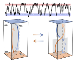
  $140< t/\tau _{ff}<200$, figure 3(c) shows that there is a ${\sim }{\rm \pi} /4$ orientation difference between the top part and the middle part, and also between the middle part and the bottom part of the LSF. At the same time, the flow strength $A$ remains well above the widely used threshold of a cessation event (Brown & Ahlers Reference Brown and Ahlers2006; Xi & Xia Reference Xi and Xia2008; Xie & Xia Reference Xie and Xia2013), i.e. 15 % of the mean flow strength as denoted by the horizontal dash-dotted line in figure 3(b), suggesting that the LSF is also well defined during this period of time. Combining the orientation and amplitude behaviour, we conjecture that the LSF is in the form of a twisted single-roll structure, which we named as the twisted LSC as sketched in figure 3(f). The corresponding $Nu$ of the LSC state and the twisted LSC state is shown in figure 3(d) with the two horizontal lines marked $Nu_H$ and $Nu_L$, respectively. It is seen that the LSC state corresponds to the $Nu_H$ state and the twisted LSC state corresponds to the $Nu_L$ state. One may note that the flow strength at the mid-height of the twisted LSC is smaller compared with that of the top and bottom heights. A similar observation when the LSF is in the form of a twisted LSC was also reported in a DNS study (Hartmann et al. Reference Hartmann, Chong, Stevens, Verzicco and Lohse2021). After going through the twisted LSC state, the orientation at different heights converges and recovers to the LSC state. The transition between two flow states causes a dramatic fluctuation of the Nusselt number.

Figure 3. An example showing the transition from the LSC state to the twisted LSC state ( $Ra=1.20\times 10^{6}$, $\varGamma =0.5$). Time trace of (a) the orientation $\theta$, (b) the flow strength $A$ and (c) the absolute value of the orientation difference between the three heights of the large-scale flow. The dash-dotted line in panel (c) is 15 % of the average of the maximum flow strength among the three heights, denoting the criterion for a flow cessation. (d) Corresponding time trace of $Nu$. Sketches of (e) the LSC state and (f) the twisted LSC state. The distributions of the UDV transducers and the velocity measurement points A and B are also depicted in panel (e). Vertical dashed lines mark the segment of different flow states.
Schindler et al. (Reference Schindler, Eckert, Zürner, Schumacher and Vogt2022) reported that the LSC will break down with increasing  $Ra$ in a cylindrical cell with $\varGamma =0.5$. They further showed that when the LSC breaks down, coherent flow states (e.g. single-roll or double-roll states) can only last for a few free-fall times. The examples shown in figure 3 suggest that both the LSC state and the twisted LSC state last for several tens of free-fall times. Thus, the large-scale flow is still in a coherent form in the present study. The different dynamics of the LSC observed from the present study and that from Schindler et al. (Reference Schindler, Eckert, Zürner, Schumacher and Vogt2022) in the $\varGamma =0.5$ cell may be due to the different range in $Ra$, i.e. the minimum value of $Ra$ studied by Schindler et al. (Reference Schindler, Eckert, Zürner, Schumacher and Vogt2022) ( $Ra=2\times 10^7$) is larger than the highest $Ra$ achieved from the present study. It should also be noted that the different cell geometries, i.e. cuboid cell in the present study and cylindrical cell in the study reported by Schindler et al. (Reference Schindler, Eckert, Zürner, Schumacher and Vogt2022), could also alter the dynamics of the LSC, as demonstrated by Ji & Brown (Reference Ji and Brown2020).
It should be noted that the orientation difference  $|\delta \theta _{bt}|$ is not always ${\rm \pi} /2$ for the twisted state. Figure 4 shows the p.d.f.s of the orientation differences between different heights when the flow is in the twisted-LSC-dominated state. A clear peak located in the range of $[{\rm \pi} /3,2{\rm \pi} /3]$ with its centre at ${\rm \pi} /2$ is obvious from the p.d.f. of $|\delta \theta _{bt}|$ shown in figure 4(a). The broad distribution of $|\delta \theta _{bt}|$ may be caused by the turbulent fluctuations in the system. Meanwhile, the p.d.f.s of $|\delta \theta _{bm}|$ and $|\delta \theta _{tm}|$ show peaks located around ${\rm \pi} /4$, which is consistent with the twisted structure illustrated in figure 3(f). Note a slight asymmetry between the peaks of $|\delta \theta _{bm}|$ and $|\delta \theta _{tm}|$ exists which can result in the asymmetry of the flow structure in the vertical plane.

Figure 4. P.d.f.s of the orientation difference between (a) the top and bottom heights, (b) the bottom and middle heights, and (c) the top and middle heights of the large-scale flow measured in the cell of  $\varGamma =0.5$.
3.2. Evolution of the flow state with increasing  $Ra$
$Ra$

It now becomes clear that the multiple states observed at  $Ra=1.20\times 10^6$ originate from different structures of the LSF, i.e. a high- $Nu$ state with a normal LSC and a low- $Nu$ state with a twisted LSC. We next study the Rayleigh number dependence of the observed phenomenon based on the measured $Nu$. Figure 5 shows $Nu$ as a function of $Ra$ measured in two convection cells with $\varGamma =0.5$ and 1. In the cell with $\varGamma =0.5$, the heat transport scaling, i.e. $Nu \sim Ra^\alpha$, shows distinctive regimes characterized by different power laws, i.e. $Nu=0.026Ra^{0.37}$ for $3.11\times 10^{5}\leq Ra \leq 6.67\times 10^{5}$ (regime I) and $Nu=0.124Ra^{0.29}$ for $1.81\times 10^{6}\leq Ra \leq 7.89\times 10^{6}$ (regime II). In the transitional range of $Ra$ between the two scaling regimes (referred to as the transitional range hereafter), a $Nu=5\times 10^{-4} Ra^{0.66}$ scaling fits the data well, as indicated by the dotted line in the figure. Analysis of the LSF structure shows that the LSF is in the form of the twisted LSC for regime I and it is in the form of the LSC in regime II, which is consistent with the fact that the $Nu$ number of regime II is larger than that of regime I when extrapolating the scaling relation obtained in regime I to regime II. In the transitional range, the data show that the flow switches between the twisted LSC state and the LSC state stochastically, similar to the example shown in figure 2(a). As the twisted LSC state and the LSC state show different values of $Nu$, the switching between the two states results in a dramatic increase in the fluctuation in $Nu$. The inset of figure 5 shows the root-mean-square value of the Nusselt number $\sigma _{Nu}$ as a function of $Ra$. Here $\sigma _{Nu}$ is defined as $\sigma _{Nu}=\sqrt {\langle (Nu(t)-\langle Nu(t)\rangle )^2\rangle }$. It is seen that in both regimes I and II, $\sigma _{Nu}$ remains very small while in the transitional range, $\sigma _{Nu}$ first increases with $Ra$, reaches a maximum and then decreases. This increase and decrease of $\sigma _{Nu}$ signatures the transition of the LSF from the LSC state to the twisted LSC state and vice versa. It should be noted that the conditioned standard deviation of $Nu$, represented by triangles in the inset of figure 5, is of the same order as when the LSF is in the form of the LSC state or the twisted LSC state. It is also seen from the inset of figure 5 that in the cell with $\varGamma =1$, $\sigma _{Nu}$ remains very close to zero, indicating that the LSF is very stable in this configuration. Meanwhile, the corresponding values of $Nu$ in the $\varGamma =1.0$ cell and that from the $\varGamma =0.5$ cell at the high $Ra$ number (the flow at the LSC state) can be fitted by a single power law, $Nu=0.124Ra^{0.29}$. This power law is in good agreement with existing data at similar $Pr$ (Naert, Segawa & Sano Reference Naert, Segawa and Sano1997; Glazier et al. Reference Glazier, Segawa, Naert and Sano1999; Zürner et al. Reference Zürner, Schindler, Vogt, Eckert and Schumacher2019; Schindler et al. Reference Schindler, Eckert, Zürner, Schumacher and Vogt2022). The solid line in figure 5 is a plot of the prediction from the Grossmann–Lohse theory (Grossmann & Lohse Reference Grossmann and Lohse2000) with updated parameters obtained from cylindrical cells (Stevens et al. Reference Stevens, van der Poel, Grossmann and Lohse2013). It is seen that the theory underestimates $Nu$. A possible reason may be due to the difference in cell geometry.

Figure 5. Log-log plot of  $Nu$ versus $Ra$ measured in convection cells with $\varGamma =0.5$ (circles) and $\varGamma =1$ (squares). The green circles in the $\varGamma =0.5$ cell stand for the averaged $Nu$ including all data measured for a given $Ra$ in the transitional range, which could be fitted by $Nu=5\times 10^{-4} Ra^{0.66}$ (the dotted line). The $Nu$ conditioned on the twisted LSC state and the LSC state in the transitional range are shown as down-pointing triangles and up-pointing triangles, respectively. The dash-dotted line is a power law fit of $Nu=0.124Ra^{0.29}$ to the data when the system is in the LSC state. The dashed line is a power law fit of $Nu=0.026Ra^{0.37}$ to the data when the system is in the twisted LSC state. The grey solid line denotes the prediction of the Grossmann–Lohse (GL) theory (Grossmann & Lohse Reference Grossmann and Lohse2000; Stevens et al. Reference Stevens, van der Poel, Grossmann and Lohse2013). The inset plots the standard deviation $\sigma _{Nu}$ of $Nu$ versus $Ra$ for the $\varGamma =0.5$ and $\varGamma =1$ cells. The $\sigma _{Nu}$ of the conditioned LSC state and conditioned twisted LSC state are also shown as up-pointing and down-pointing triangles, respectively.
Detailed examination of the flow structure using the temperature profiles measured inside the sidewall shows that the LSF is in the LSC state in the cell with  $\varGamma =1$. This can be seen clearly from figure 6, where we plot the normalized flow strength $A_m$ of the LSF measured at the mid-height of the cell. It is seen that in the cell with $\varGamma =1$, $A_m/\Delta T$ decreases with $Ra$. In the cell with $\varGamma =0.5$, however, $A_m/\Delta T$ first increases with $Ra$ and starts to decrease with $Ra$ for $Ra>1.62\times 10^{6}$. The transitional $Ra$ of $A_m/\Delta T$ is similar to the transitional $Ra$ observed from the Nusselt number measurements shown in figure 5, suggesting that the transition of the flow state occurs concurrently with the transition of the heat transport efficiency. Note, in both cells, the decrease of $A_{m}/\Delta T$ with $Ra$ can be fitted by a single power law, i.e. $A_m/\Delta T\sim Ra^{-0.14}$. This can be regarded as consistent with the observed unified power law relation between $Nu$ and $Ra$ for the LSC state shown in figure 5.

Figure 6. Normalized flow strength  $A_m/\Delta T$ at the mid-height versus $Ra$. The dashed line represents a power law fitting to the data, i.e. $A_{m}/\Delta T=2.12Ra^{-0.14}$.
3.3. Flow dynamics in the transitional range
The switching between the LSC state and the twisted LSC state is a distinct feature of the transitional range. To further understand the dynamics of this switching, we study the time percentage of the the LSC state and the twisted LSC state, and the time interval between them. The following algorithm was used to identify different flow states based on the time series of  $Nu(t)$. If $Nu(t)> Nu_H-\sigma _{Nu_H}$, the flow is classified as the LSC state. If $Nu(t)< Nu_L+\sigma _{Nu_L}$, the flow is classified as the twisted LSC state (see red and blue shadows in figure 2a). The rest of the time is classified as the transitional state.
Figure 7 shows the time percentage  $w$ when the flow stays in different states. It is seen that at the low end of $Ra$, the flow is dominated by the twisted LSC state. With increasing $Ra$, the time percentage $w$ of the LSC state gradually increases and becomes dominant for the highest $Ra$ in the transitional range. Meanwhile, the time percentage $w$ of the twisted LSC state decreases with increasing $Ra$ and becomes close to zero at the highest $Ra$ in the transitional range. The time percentage $w$ of the transitional state depends weakly on $Ra$ as revealed by the squares in figure 7(a). Figure 7(b) plots the normalized mean lifetime $t_w/\tau _{ff}$ of the three states. Despite the data being of scatter, one sees that $t_w/\tau _{ff}$ seems to be independent of $Ra$ with a mean value of ${\sim }60 \tau _{ff}$ for the transitional state, and ${\sim }40 \tau _{ff}$ for the twisted LSC state and the LSC state.

Figure 7. (a) The time percentage of the flow stays at the twisted LSC state, transitional state and the LSC state in the transitional range. (b) Normalized mean lifetime of the three states in the transitional range.
The observed twisted LSC state reminds one of the twisting oscillation of the planar LSC observed in turbulent RBC (Xi et al. Reference Xi, Zhou, Zhou, Chan and Xia2009; Weiss & Ahlers Reference Weiss and Ahlers2011; Zwirner et al. Reference Zwirner, Khalilov, Kolesnichenko, Mamykin, Mandrykin, Pavlinov, Shestakov, Teimurazov, Frick and Shishkina2020a). However, the twisted LSC state observed in the present study is different from the twisting oscillation in terms of their time scale. For example, at  $Ra=1.42\times 10^7$, the twisting oscillation period reported by Zwirner et al. (Reference Zwirner, Khalilov, Kolesnichenko, Mamykin, Mandrykin, Pavlinov, Shestakov, Teimurazov, Frick and Shishkina2020a) is ${\sim }9.2\tau _{ff}\approx 12s$. The LSC turn-over time estimated based on the velocity measurement reported by Khalilov et al. (Reference Khalilov, Kolesnichenko, Pavlinov, Mamykin, Shestakov and Frick2018) is $\tau _{LSC}=(4H)/(v_{LSC})=4\times 0.216/0.063 s\approx 14s$. One sees that the twisting oscillation is of the same time scale as the LSC turn-over time ( ${\sim }0.9\tau _{LSC}$). In the present study, the twisted LSC state lasted approximately 40 $\tau _{ff}$ at $Ra=1.20\times 10^6$. The LSC turn-over time estimated from the direct velocity measurement performed using ultrasonic Doppler velocimetry is $\tau _{LSC}=(2D+2H)/(v_{LSC})=(2\times 0.05+2\times 0.103)/0.004s\approx 76s$, which is approximately 14.5 $\tau _{ff}$. Thus, the twisted LSC lasted approximately 3 $\tau _{LSC}$. The difference between the time scale of the twisted LSC and that of the twisting oscillation suggests that they have different flow dynamics occurring on different time scales. Thus the twisted LSC and the twisting oscillation of the LSC are two different natures of the LSF in liquid metal convection. It is worthy mentioning that, unlike the periodic motion of the twisting oscillation, the occurrence of the twisted LSC state is not periodic. One should notice that the twisted LSC state is a flow structure, which is different from the dynamical switching of the LSC plane between different body diagonals of a cubic cell, such as those reported by Ji & Brown (Reference Ji and Brown2020).
3.4. Temperature fluctuation at the cell centre for different flow states
To further shed light upon the difference between flow states in cells with  $\varGamma =0.5$ and $\varGamma =1$ when $Ra$ is the same, we study the temperature fluctuations at the cell centre. Figures 8(a) and 8(b) plot the time trace of the normalized temperature fluctuation $(T_{c}-\langle T_{c} \rangle )/\sigma _{T_{c}}$ at $Ra=5\times 10^5$ for cells with $\varGamma =1$ and $\varGamma =0.5$, respectively. From the heat transport data shown in figure 5, one knows that the LSF is in the form of the normal LSC state in the $\varGamma =1$ cell and it is in the form of the twisted LSC state in the $\varGamma =0.5$ cell. It is seen that there exist sharp spikes in the time trace of the temperature fluctuation in the $\varGamma =1$ cell, which could be conjectured as signatures of thermal plumes (Shang et al. Reference Shang, Qiu, Tong and Xia2004). However, the temperature fluctuation time trace shows that temperature fluctuation is confined between $\langle T \rangle \pm 2.5\sigma _{T}$ in the $\varGamma =0.5$ cell. The difference in the nature of temperature fluctuation can be seen more clearly from their respective p.d.f.s shown in figure 8(c). It is seen that the largest temperature fluctuations can reach almost $\langle T \rangle \pm 5\sigma _{T}$ in the $\varGamma =1$ cell. However, it only reaches $\langle T \rangle \pm 2.5\sigma _{T}$ in the $\varGamma =0.5$ cell.

Figure 8. Time series of normalized temperature fluctuations measured in the centre of (a) the  $\varGamma =1$ and (b) the $\varGamma =0.5$ cell at $Ra=5\times 10^{5}$. (c) P.d.f. of the standardized temperature fluctuation at the cell centre.
To quantify the difference in the temporal dynamics of the temperature fluctuation. We study their power spectra density (PSD). Figures 9(b) and 9(c) show the PSD of  $T_c$ measured in cells with $\varGamma =1.0$ and $\varGamma =0.5$, respectively. To compare the PSD from different $Ra$, the frequency axis is normalized by the peak frequency $f_p$ obtained from the dissipation spectra, i.e. $f^2P(\,\textit{f}\,)$ versus $f$ (She & Jackson Reference She and Jackson1993; Zhou & Xia Reference Zhou and Xia2001). Here, $f^2P(\,\textit {f}\,)$ is calculated based on the original PSD of the temperature at the cell centre shown in figure 9(a). The dissipation PSD is shown in the inset of figure 9(a). In figures 9(b) and 9(c), the vertical axis is normalized by the value of the PSD corresponding to $f_p$. It is seen from figure 9(b) that the normalized PSD in the cell with $\varGamma =1$ for different values of $Ra$ show a universal shape. In addition, the PSDs in the $\varGamma =1$ cell show two scaling regimes characterized by $P(\,f)/P(\,f_p)\sim (\,f/f_p)^{-5/3}$ and $P(\,f)/P(\,f_p)\sim (\,f/f_p)^{-17/3}$. The appearance of the two scaling regimes indicates that the flow in the studied parameter range is in the form of developed turbulence (Batchelor, Howells & Townsend Reference Batchelor, Howells and Townsend1959). This is consistent with the recent study reporting that the flow will be turbulent when $Ra>1.0\times 10^5$ in liquid metal convection with $\varGamma =1$ (Ren et al. Reference Ren, Tao, Zhang, Ni, Xia and Xie2022). The PSDs measured in the cell with $\varGamma =0.5$ show different behaviours. It is seen from figure 9(c) that the shape of the normalized PSDs changes with increasing $Ra$. For $Ra<5.0\times 10^5$, the PSDs show no evidence of developed turbulence. When $Ra>3.5\times 10^6$, the PSDs show two scaling regimes similar to the cell with $\varGamma =1$. The observation suggests that in the cell with $\varGamma =0.5$, when $Ra$ is increased from the lowest end of the studied parameter range, the flow gradually evolves to the fully developed turbulence state with a single roll LSC for $Ra>1.80\times 10^{6}$.

Figure 9. (a) Original temperature PSD at the cell centre for the same  $Ra$ of panel (b) in the $\varGamma =1$ cell. The inset shows the temperature dissipation spectrum and its peak value $f_{p}$. The scaled temperature power spectrum density (PSD) for various $Ra$ in the cell with (b) $\varGamma =1$ and (c) $\varGamma =0.5$. The dashed lines in panel (b,c) indicate two scaling regimes, i.e. inertial-convective subrange with $P(\,{f})\sim f^{-5/3}$ and inertial-conductive subrange with $P(\,{f})\sim f^{-17/3}$.
The change in the shape of the PSDs in the  $\varGamma =0.5$ cell and the $Ra$-dependence of the flow strength can be regarded as being consistent with the heat transport data shown in figure 5. When $Ra<1.80\times 10^{6}$, the bulk flow is in the turbulence state in the cell with $\varGamma =1$. However, the flow is in the regime before the transition to fully developed turbulence in the cell with $\varGamma =0.5$. This difference in the bulk flow state could possibly originate from the strength of the LSF. As it is seen from figure 6, the flow strength of the LSC is larger than that of the twisted LSC. The turbulence at the cell centre gains energy from the shear produced by the LSF (Xia, Sun & Zhou Reference Xia, Sun and Zhou2003). A stronger LSC will result in a more turbulent flow. In addition, there exists bistability when the system gradually evolves towards fully developed turbulence in the cell with $\varGamma =0.5$. The PSDs continuously evolve with $Ra$ and show two slopes when $Ra>2\times 10^6$, implying that the flow will become fully developed for $Ra>2\times 10^6$.
4. Conclusion
We show experimentally that the heat transport in low-Prandtl-number thermal convection can show intriguing dependence on the flow structures. In a cell with  $\varGamma =0.5$, the large-scale flow exhibits two states: a twisted LSC state with its heat transport efficiency being ${\sim }35\,\%$ smaller than a normal LSC state. The twisted LSC state differs from the twisting oscillation in terms of its time scale. With increasing the level of turbulence, the system gradually evolves from the twisted LSC state with $Nu\sim Ra^{0.37}$ to the LSC state with $Nu\sim Ra^{0.29}$. Bistability is observed before the system becomes fully developed turbulence for $Ra>1.80\times 10^6$. Combining measurements in cells with $\varGamma =1$ and 0.5, the study shows that the large-scale flow exhibits a self-similar LSC structure when the system is in the fully developed turbulence state, characterized by a universal power law for the heat transport, i.e. $Nu\sim Ra^{0.29}$. The study demonstrates experimentally that a strong coupling between the large-scale flow and heat transport exits in low-Pr-number thermal convection, which makes it possible to control heat transport via tuning of the large-scale flow in convection.
Funding
This work is supported by National Natural Science Foundation (NSFC) under grant numbers 51927812, 92152104, 52176086, 12002260 and 52222607, the National Key R&D Program of China under grant number 2022YFE03130000 and Fundamental Research Funds for the Central Universities (xzy012021005).
Declaration of interests
The authors report no conflict of interest.
Author contributions
X.-Y. Chen and Y.-C. Xie contributed equally to this work.


