


1. Introduction
We consider the Brownian motion of a colloidal rigid particle in a binary fluid mixture lying in the homogeneous phase near the demixing critical point. In some combinations of the mixture and particle material, one of the components is preferentially attracted by the particle surface and the preferred component is remarkably adsorbed near the particle surface because of the near-criticality (Beysens & Leibler Reference Beysens and Leibler1982; Beysens & Estève Reference Beysens and Estève1985). The particle motion deforms the adsorption layer, which affects the force exerted on the particle (Lee Reference Lee1976; Omari, Grabowski & Mukhopadhyay Reference Omari, Grabowski and Mukhopadhyay2009; Okamoto, Fujitani & Komura Reference Okamoto, Fujitani and Komura2013; Fujitani Reference Fujitani2018; Tani & Fujitani Reference Tani and Fujitani2018; Yabunaka & Fujitani Reference Yabunaka and Fujitani2020). In other combinations exhibiting negligible preferential adsorption, the particle motion remains still influenced by the near-criticality because of the critical enhancement of the viscosity (Ohta Reference Ohta1975; Ohta & Kawasaki Reference Ohta and Kawasaki1976). This enhancement can also be influenced by the particle motion, as is pointed out in a recent experimental work (Beysens Reference Beysens2019). We briefly mention its background in some paragraphs below.
Let us first assume there are no particles in an equilibrium near-critical binary fluid mixture. The composition can be represented by the difference between (or the ratio of) the mass densities of the two components. The order parameter, which we can take to be proportional to the deviation of the local composition from the critical one, fluctuates about the equilibrium value on length scales smaller than the correlation length,  $\xi$. Correlated clusters, where the order parameter keeps the same sign on average, range over these scales, and are convected to enhance the interdiffusion of the components on larger length scales (Kawasaki Reference Kawasaki1970; Onuki Reference Onuki2002). Thus, $\xi$ affects how the two-time correlation function of the order-parameter fluctuation decays. Writing $\varGamma _k$ for the relaxation coefficient of its spatial Fourier transform, with $k$ denoting the magnitude of the wavenumber vector, we have
 \begin{equation} \varGamma_k=\varOmega(k\xi) \times k^{z}, \end{equation}
for small  $k$ with $k\xi$ being finite. Here, $z$ denotes the dynamic critical exponent for the order-parameter fluctuation and $\varOmega$ represents a scaling function, which approaches a constant multiplied by $(k\xi )^{2-z}$ as $k\xi$ becomes much smaller than unity (Siggia, Hohenberg & Halperin Reference Siggia, Hohenberg and Halperin1976; Hohenberg & Halperin Reference Hohenberg and Halperin1977). This leads to $\varGamma _k\propto k^2$ for sufficiently small $k$, which is expected for the hydrodynamic mode of a conserved quantity. We write $k_{B}$ for the Boltzmann constant and $T$ for the temperature of the mixture. The mode-coupling theory for a three-dimensional mixture gives
 \begin{equation} \varOmega(k\xi)=\frac{k_{B}T}{6{\rm \pi}\tilde{\eta}} \frac{K(k\xi)}{(k\xi)^3}, \end{equation}
where  $K$ denotes the Kawasaki function with $K(x)\approx 3{\rm \pi} x^3/8$ for $x\gg 1$ and $K(x)\approx x^2$ for $x\ll 1$, and $\tilde {\eta }$ represents the shear viscosity (Kawasaki Reference Kawasaki1970; Onuki Reference Onuki2002). In this theory, the weak critical singularity of the viscosity is neglected, and the dynamic critical exponent is found to be three. This theoretical result turns out to be in good agreement with the experimental results (Swinney & Henry Reference Swinney and Henry1973). In the refined calculation of the dynamic renormalization group, the critical enhancement of $\tilde {\eta }$ is considered, and the value of $z$ is found to be slightly larger than three (Folk & Moser Reference Folk and Moser2006).
The mixture is assumed to be at equilibrium in the preceding paragraph. The critical enhancement of the transport coefficients, i.e. the Onsager coefficient for the interdiffusion and the shear viscosity, can be suppressed when a shear is imposed on the mixture. Influences of a simple shear flow are studied theoretically (Onuki & Kawasaki Reference Onuki and Kawasaki1979; Onuki, Yamazaki & Kawasaki Reference Onuki, Yamazaki and Kawasaki1981) and experimentally (Beysens, Gbadamassi & Boyer Reference Beysens, Gbadamassi and Boyer1979; Beysens & Gbadamassi Reference Beysens and Gbadamassi1980). In an example of this flow, the  $x$ component of the velocity is $y$ multiplied by the constant shear rate $s\,(>\!0)$, with $(x,y)$ denoting two of the three-dimensional Cartesian coordinates. A correlated cluster of the order-parameter fluctuation would be deformed by the shear when its lifetime is longer than a typical time scale of the shear, $1/{s}$. The lifetime for a cluster with the size of $1/k$ is evaluated to be $1/\varGamma _k$, while the cluster size ranges up to $\xi$. Hence, if the shear is strong enough to satisfy
 \begin{equation} {s}>\varGamma_{1/\xi}, \end{equation}
the enhancement is suppressed. This condition of strong shear is also derived in terms of the renormalization group, as mentioned in appendix A.
A simple shear flow is a kind of linear shear flow, where the velocity  $\boldsymbol {V}$ at a position is proportional to the positional vector, and can be regarded as a linear combination of a stagnation-point flow and a purely rotational flow (Rallison Reference Rallison1984). These linear shear flows are two-dimensional. A pure-extension flow, being a three-dimensional linear shear flow, and a stagnation-point flow are referred to as elongational flows in Onuki & Kawasaki (Reference Onuki and Kawasaki1980a,Reference Onuki and Kawasakic), where the suppression is studied for some linear shear flows. In a linear shear flow, the time derivative of a directed line segment $\boldsymbol {X}$ linking two fluid particles is equal to $(\boldsymbol {\nabla } \boldsymbol {V})^\textrm {T}\boldsymbol {\cdot } \boldsymbol {X}$, where the matrix $\boldsymbol {\nabla } \boldsymbol {V}$ represents the homogeneous velocity gradient and superscript $\textrm {T}$ indicates the transposition. Thus, the exponential of the product of $(\boldsymbol {\nabla } \boldsymbol {V})^\textrm {T}$ and the time $t$ determines how $\boldsymbol {X}$ is stretched and shrunk with time. In the elongational flow, the shear rate $s$ in (1.3) is given by the largest stretching rate, i.e. the largest eigenvalue of $\boldsymbol {\nabla } \boldsymbol {V}$; some details are mentioned in the penultimate paragraph of appendix A.
The mean square displacement of a Brownian particle becomes proportional to the time interval as it becomes sufficiently long. The self-diffusion coefficient of the particle is defined as the constant of proportionality divided by twice the spatial dimension. In the study mentioned at the end of the first paragraph (Beysens Reference Beysens2019), it is shown that the self-diffusion coefficient of a Brownian particle in a near-critical binary fluid mixture first decreases and then reaches a plateau as  $T$ approaches the critical temperature $T_{c}$ along the critical isochore in the homogeneous phase. The first decrease should reflect the critical enhancement of $\tilde {\eta }$, while the plateau can be regarded as representing the suppression of the enhancement due to the shear caused by the particle motion. Using (1.2) and replacing $s$ in (1.3) with the average particle speed divided by the particle radius, Beysens (Reference Beysens2019) estimates the temperature range exhibiting the suppression; the estimated range appears consistent with the observed one. In the present study, we calculate the self-diffusion coefficient for direct comparison with the experimental results.
In the first three subsections of § 2, we calculate the hydrodynamic force exerted on a rigid spherical particle moving translationally in a fluid mixture quiescent far from the particle. Assuming a typical length scale of the flow to be much larger than  $\xi$, we need not consider dynamics of the order-parameter fluctuation, which is significant only on length scales smaller than $\xi$ (Furukawa et al. Reference Furukawa, Gambassi, Dietrich and Tanaka2013; Okamoto et al. Reference Okamoto, Fujitani and Komura2013). The mixture is assumed to be incompressible, as in the previous studies mentioned above (Folk & Moser Reference Folk and Moser1998; Onuki Reference Onuki2002). This assumption usually works well in a near-critical mixture prepared experimentally (Anisimov et al. Reference Anisimov, Gorodetskii, Klikov and Sengers1995; Onuki Reference Onuki2002; Pérez-Sanchez et al. Reference Pérez-Sanchez, Losada-Pérez, Cerdeiriña, Sengers and Anisimov2010). When the viscosity is homogeneous, the magnitude of the force is proportional to the particle speed. The constant of proportionality (the drag coefficient) is given by Stokes’ law (Stokes Reference Stokes1851) and is linked with the self-diffusion coefficient of its Brownian motion through the Sutherland–Einstein relation (Einstein Reference Einstein1905; Sutherland Reference Sutherland1905), although the Brownian motion is not always translational. This relation can be derived from the Langevin equation for the particle velocity (Bian, Kim & Karniadakis Reference Bian, Kim and Karniadakis2016), and is further founded on the fluctuating hydrodynamics (Bedeaux & Mazur Reference Bedeaux and Mazur1974), even near the critical point (Mazur & van der Zwan Reference Mazur and van der Zwan1978). In our problem, the suppression of the viscosity enhancement is locally determined by the inhomogeneous shear around the particle, and the drag coefficient can depend on the particle speed in its range to be considered in the Brownian motion. Neither Stokes’ law nor the Sutherland–Einstein relation is applicable when the suppression occurs. Assuming the suppression to remain weak even if it is brought about by the local strong shear, we calculate the drag coefficient. In § 2.4, we use a one-dimensional Langevin equation to link the drag coefficient with the self-diffusion coefficient. Our results are shown and discussed in § 3, and summarized in § 4.
2. Formulation and calculation
We write  $d$ for the spatial dimension; our calculations in the text are limited to the case of $d=3$. The values of the static critical exponents are shown in Pelisetto & Vicari (Reference Pelisetto and Vicari2002); we use $\nu \approx 0.630$ and $\eta \approx 0.0364$. The exponent $\eta$ represents the deviation from the straightforward dimensional analysis of the static, or equal time, correlation function of the order-parameter fluctuation at the critical point. When the shear is not so strong as to suppress the critical enhancement, the correlation length $\xi$ is homogeneously given by $\xi =\xi _0\tau ^{-\nu }$ on the critical isochore, where $\tau$ is defined as $|T-T_{c}|/T_{c}$ and $\xi _0$ is a non-universal constant. Then, the singular part of the shear viscosity is proportional to $\tau ^{\nu (d-z)}$ in a flow whose typical length is much larger than $\xi$, as described at (A 2). This exponent is measured to be around $-0.042$ (Berg & Moldover Reference Berg and Moldover1989, Reference Berg and Moldover1990), which leads to $z=3.067$. Because $|\nu (d-z)|$ is small, the viscosity exhibits a very weak critical singularity. Thus, for the viscosity, the dependence of the regular part on $\tau$ is also significant unless the mixture is very close to the critical point, unlike for the Onsager coefficient of the interdiffusion. As in Beysens (Reference Beysens2019), we use
 \begin{equation} \tilde{\eta}_{B}(T) \tau^{\nu (d-z)} \end{equation}
as the viscosity free from the shear effects. In this form of multiplicative anomaly, the regular part  $\tilde {\eta }_{B}$ is defined as
 \begin{equation} \tilde{\eta}_{B}(T)=\tilde{\eta}_0 \exp{\left(\frac{E_{a}}{k_{B}T}\right)}, \end{equation}
where  $\tilde {\eta }_0$ is a non-universal constant and $E_{a}$ denotes the activation energy (Sengers Reference Sengers1985; Mehrotra, Monnery & Svrcek Reference Mehrotra, Monnery and Svrcek1996). Molecules would be required to overcome some energy barrier to shift their locations in a dense liquid. Equation (2.1) supposes $\tau <1$ and the singular part represents the enhancement.
We define  $\tau _s$ so that a given shear rate ${s}$ affects the critical enhancement for $\tau <\tau _s$, and define $s^*$ so that
 \begin{equation} \tau_s= \left(\frac{s}{s^*}\right)^{1/(\nu z)} \end{equation}
holds. Because of (1.1) and (1.3),  $s^*$ is independent of the imposed shear. We will later apply our results to a mixture of isobutyric acid and water. For this mixture under no shear, measured values of $\varGamma _k/k^2$ for small $k$ in the neighbourhood of the critical point are shown in figure 10 of Chu, Schoenes & Kao (Reference Chu, Schoenes and Kao1968). These values and $\xi _0=0.3625\ \textrm {nm}$ (Beysens, Bourgou & Calmettes Reference Beysens, Bourgou and Calmettes1985) give $s^*=3.7\times 10^8\ \textrm {s}^{-1}$ with the aid of (A 4) and (A 6).
From § 2.1 to § 2.3, we calculate the drag coefficient of a spherical rigid particle with radius  $r_0$, by assuming it to move translationally with the velocity $U\boldsymbol {e}_z$ in a binary fluid mixture in the absence of the preferential adsorption (figure 1). Here, $\boldsymbol {e}_z$ denotes a unit vector. The mixture is on the critical isochore in the homogeneous phase with $T$ being close to $T_{c}$, and is quiescent far from the particle. Assuming $\xi$ to be much smaller than a typical length scale that the flow changes, we regard the local velocity field as a linear shear flow having the same velocity gradient to determine the local viscosity.

Figure 1. A drawing of a situation for our calculation of the drag coefficient from § 2.1 to § 2.3. A particle with the radius  $r_0$ moves translationally with the velocity $U\boldsymbol {e}_z$ in a mixture fluid quiescent far from the particle. A part of a cross-section containing the $z$ axis is shown; the dashed curve represents half of the cross-section of the particle surface. The velocity field, represented by arrows outside the particle, is calculated with a homogeneous viscosity, although the viscosity becomes inhomogeneous when the suppression of the critical enhancement occurs somewhere. A magnified view of the smaller rectangular region is given in the larger one, where clusters are schematically drawn in black and white with some being deformed by the local shear. The correlation length $\xi$ is assumed to be sufficiently small as compared with a typical length of the flow.
2.1. Assumption on the viscosity
We assume that the suppression of the critical enhancement of  $\tilde {\eta }$ is perfect if it occurs, and thus the viscosity is assumed to be given by
 \begin{equation} \tilde{\eta}=\begin{cases} \tilde{\eta}_{B}(T) \tau^{\nu (d-z)} & \textrm{for}\ \tau>\tau_s,\\ \tilde{\eta}_{B}(T) \tau_s^{\nu (d-z)} & \textrm{for}\ \tau< \tau_s, \end{cases}\end{equation}
which supposes  $\tau <1$ and $\tau _s<1$ because (2.1) underlies (2.4). This assumption is discussed in § 3. We write $\tilde {\eta }^{(0)}$ for (2.1), and define $\tilde {\eta }^{(1)}$ so that $\tilde {\eta }=\tilde {\eta }^{(0)}+\tilde {\eta }^{(1)}$ holds. Introducing $\check {\tau }_s\equiv \tau _s/\tau$, we have
 \begin{equation} \tilde{\eta}^{(1)}\equiv \tilde{\eta}^{(0)}\left( \check{\tau}_s^{\nu (d-z)}- 1\right)\varTheta(\check{\tau}_s-1), \end{equation}
where  $\varTheta$ denotes the step function; $\varTheta (x)$ vanishes for $x<0$ and equals unity for $x>0$. The shear rate is inhomogeneous, as shown later. Thus, the suppression makes the viscosity inhomogeneous. Subtracting the homogeneous part $\tilde {\eta }^{(0)}$ from the whole viscosity $\tilde {\eta }$ gives $\tilde {\eta }^{(1)}$, which is non-positive because of $d=3<z$.
The velocity and pressure fields,  $\boldsymbol {v}$ and $p$, satisfy the incompressibility condition and Stokes’ equation, i.e.
 \begin{equation} \boldsymbol{\nabla}\boldsymbol{\cdot}\boldsymbol{v}=0\quad\textrm{and}\quad -\boldsymbol{\nabla} p+ 2\boldsymbol{\nabla}\boldsymbol{\cdot} \left(\tilde{\eta} \boldsymbol{\boldsymbol{\mathsf{E}}}\right)=0, \end{equation}
where  $\boldsymbol{\boldsymbol{\mathsf{E}}}$ is the rate-of-strain tensor. Here, a low Reynolds number is assumed, as discussed in § 2 of Yabunaka & Fujitani (Reference Yabunaka and Fujitani2020). The no-slip boundary condition is imposed at the particle surface, while $\boldsymbol {v}$ tends to zero and $p$ approaches a constant, denoted by $p_{\infty }$, far from the particle.
2.2. Approximation for a weak suppression
We consider a particular time and take the spherical coordinates  $(r,\theta ,\phi )$ so that the origin is at the particle's centre and that the polar axis ( $z$ axis) is along $\boldsymbol {e}_z$; the coordinate $z$ should not be confused with the dynamic critical exponent. The unit vectors in the directions of $r$ and $\theta$ are denoted by $\boldsymbol {e}_r$ and $\boldsymbol {e}_{\theta }$, respectively. The no-slip condition gives $\boldsymbol {v}=U\boldsymbol {e}_z$ at $\rho =1$, where $\rho$ denotes a dimensionless radial distance, $r/r_0$. We can assume $v_{\phi }=0$. The drag force is along the $z$ axis; its $z$ component, denoted by $\mathcal {F}_z$, is given by the surface integral of $(2\tilde {\eta } \boldsymbol{\boldsymbol{\mathsf{E}}} \boldsymbol {\cdot } \boldsymbol {e}_r - p\boldsymbol {e}_r)\boldsymbol {\cdot }\boldsymbol {e}_z$ over the particle surface. The drag coefficient is given by $-\mathcal {F}_z/U$, and can depend on $U$ in our problem. Thus, we write $\gamma (U)$ for the drag coefficient.
We, respectively, write  $\boldsymbol {v}^{(0)}$ and $p^{(0)}$ for the velocity and pressure fields obtained when the viscosity is forced to be $\tilde {\eta }^{(0)}$ homogeneously. Equation (2.6a,b) yields
 \begin{equation} \boldsymbol{\nabla}\boldsymbol{\cdot}\boldsymbol{v}^{(0)}=0 \quad\textrm{and}\quad -\boldsymbol{\nabla} p^{(0)}+ \tilde{\eta}^{(0)} \Delta \boldsymbol{v}^{(0)}=0. \end{equation}
The boundary conditions are  $\boldsymbol {v}^{(0)}=U\boldsymbol {e}_z$ at $\rho =1$, and $\boldsymbol {v}^{(0)}\to \boldsymbol {0}$ and $p^{(0)}\to p_{\infty }$ as $\rho \to \infty$. The solution is well known (Stokes Reference Stokes1851) and is given by
 \begin{align} p^{(0)}=p_{\infty}+\frac{3\tilde{\eta}^{(0)}}{2r_0 \rho^2}U\cos{\theta},\quad v_r^{(0)}=\frac{3\rho^2-1}{2\rho^3}U\cos{\theta},\quad v_{\theta}^{(0)}=-\frac{3\rho^2+1}{4\rho^3}U\sin{\theta} \end{align}
and  $v_{\phi }^{(0)}=0$. The arrows outside the particle in figure 1 represent $\boldsymbol {v}^{(0)}$ for $U>0$. The superscript ${(0)}$ is also added to a quantity calculated from $\boldsymbol {v}^{(0)}$ and $p^{(0)}$. The drag coefficient calculated from (2.8a–c) is given by
 \begin{equation} \gamma^{(0)}= -\frac{\mathcal{F}_z^{(0)}}{U} = 6{\rm \pi}\tilde{\eta}^{(0)}r_0, \end{equation}
which is independent of  $U$ and represents Stokes’ law. We define $\boldsymbol {v}^{(1)}$ and $p^{(1)}$ as $\boldsymbol {v}-\boldsymbol {v}^{(0)}$ and $p-p^{(0)}$, respectively. They satisfy $\boldsymbol {\nabla }\boldsymbol {\cdot }\boldsymbol {v}^{(1)}=0$ and
 \begin{equation} -\boldsymbol{\nabla} p^{(1)}+ \tilde{\eta}^{(0)} \Delta \boldsymbol{v}^{(1)}=-2\boldsymbol{\nabla}\boldsymbol{\cdot} \left(\tilde{\eta}^{(1)}\boldsymbol{\boldsymbol{\mathsf{E}}}\right). \end{equation}
The boundary conditions are
 \begin{equation} \left. \begin{gathered} \boldsymbol{v}^{(1)}=\boldsymbol{0} \quad \textrm{at}\ \rho=1 \quad\textrm{and}\\ \boldsymbol{v}^{(1)}\to \boldsymbol{0}\quad \textrm{and}\quad p^{(1)}\to 0\quad \textrm{as}\ \rho\to\infty. \end{gathered} \right\} \end{equation}
 In the flow field of  $\boldsymbol {v}$ and $p$, we define $\kappa$ as the maximum value of a dimensionless ratio $|\tilde {\eta }^{(1)}/\tilde {\eta }^{(0)}|$. Equation (2.5) is proportional to $\kappa$. From (2.10) and (2.11), $\boldsymbol {v}^{(1)}$ is also proportional to $\kappa$. The particle speed supposed here lies in the range involved in the Brownian motion. We assume that $\tau$ is not so small as to cause strong suppression, and assume $\kappa$ to be so small that the calculation up to the order of $\kappa$ makes sense. At this order, (2.10) becomes
 \begin{equation} -\boldsymbol{\nabla} p^{(1)}+ \tilde{\eta}^{(0)} \Delta \boldsymbol{v}^{(1)}=-\tilde{\eta}^{(1)}\Delta\boldsymbol{v}^{(0)} -\left(2\boldsymbol{\nabla}\tilde{\eta}^{(1)}\right)\boldsymbol{\cdot} \boldsymbol{\boldsymbol{\mathsf{E}}}^{(0)}. \end{equation}
Here,  $s$ contained in $\tilde {\eta }^{(1)}$ is replaced by $s^{(0)}$, which is the shear rate calculated from $\boldsymbol {v}^{(0)}$. Likewise, we can evaluate $\kappa$ by using $s^{(0)}$ instead of $s$ in (2.5). We define $\mathcal {F}_z^{(1)}$ so that $\mathcal {F}_z=\mathcal {F}_z^{(0)}+\mathcal {F}_z^{(1)}$ holds. At the order of $\kappa$, $\mathcal {F}_z^{(1)}$ equals the surface integral of
 \begin{equation} 2\tilde{\eta}^{(1)} \boldsymbol{\boldsymbol{\mathsf{E}}}^{(0)}_{rz}+2\tilde{\eta}^{(0)} \boldsymbol{\boldsymbol{\mathsf{E}}}^{(1)}_{rz}-p^{(1)}\boldsymbol{e}_r\boldsymbol{\cdot}\boldsymbol{e}_z \end{equation}
over the particle surface, where  $\boldsymbol{\boldsymbol{\mathsf{E}}}^{(1)}$ is the rate-of-strain tensor for $\boldsymbol {v}^{(1)}$ and $p^{(1)}$.
On the  $z$ axis, the components of $\boldsymbol {\nabla } \boldsymbol {v}^{(0)}$ with respect to the Cartesian coordinates $(x,y,z)$ is expressed by $\partial _zv^{(0)}_z$ multiplied by a traceless diagonal matrix, whose diagonal elements are $-1/2, -1/2$ and $1$ from the top. Here, $\partial _z$ indicates the partial derivative with respect to $z$. Thus, noting the description at the end of the preface of § 2, we can regard $\boldsymbol {v}^{(0)}$ on the $z$ axis as a pure-extension flow locally. In particular, at a point with $\theta ={\rm \pi}$ for $U>0$, the largest stretching rate occurs in the $z$ direction, i.e. the radial direction, and is given by $\partial _r v^{(0)}_r$. As $\theta$ approaches ${\rm \pi} /2$, periodic motion becomes predominant over elongational motion in $\boldsymbol {v}^{(0)}$, as is suggested by figure 1 and is explicitly shown in appendix B. A rotational flow is found to be weak in suppressing the critical enhancement (Onuki & Kawasaki Reference Onuki and Kawasaki1980c). Thus, considering the discussion on the elongational flow in the fourth paragraph of § 1, we assume that $s^{(0)}$ is given by the largest real-part of the eigenvalues of $\boldsymbol {\nabla }\boldsymbol {v}^{(0)}$. Calculating them directly from (2.8a–c), we find $s^{(0)}$ to be given by
 \begin{equation} s^{(0)}(\rho,\theta)=\left| \frac{3{c} U}{4r_0} \left(\frac{1}{\rho^{2}}-\frac{1}{\rho^{4}}\right)\cos{\theta}\right|, \end{equation}
where a positive factor  ${c}$, depending on $\theta$, ranges from $1/2$ to $2$. Equation (2.14) with ${c}=2$ equals $\vert \partial _r v^{(0)}_r\vert$. We proceed below with calculations by regarding ${c}$ as a constant, in spite of the actual dependence of $c$ on $\theta$. It will be shown later that our result of the self-diffusion coefficient is rather insensitive to the value of ${c}$.
2.3. Expansions with respect to the spherical harmonics
The flow we consider here is symmetric with respect to the polar axis, and thus the angular part of  $\boldsymbol {v}^{(1)}$ can be expanded in terms of the vector spherical harmonics,
 \begin{equation} \boldsymbol{P}_{J0} = Y_{J0} \boldsymbol{e}_r\quad\textrm{and}\quad \boldsymbol{B}_{J0}=\frac{r\boldsymbol{\nabla} Y_{J0}}{\sqrt{J(J+1)}} \end{equation}
for  $J=1,2,\ldots$ (Morse & Feshbach Reference Morse and Feshbach1953; Barrera, Estévez & Giraldo Reference Barrera, Estévez and Giraldo1985; Fujitani Reference Fujitani2007). Here, $Y_{J0}(\theta )$ is one of the spherical harmonics, $\sqrt {(2J+1)/(4{\rm \pi} )}P_J(\cos {\theta })$, with $P_J$ denoting the Legendre polynomial, e.g. $P_1(x)=x$. The mode $J=0$ need not be considered because of the incompressibility. We define functions $\varPi _J$, $R_J$ and $T_J$ so that
 \begin{equation} p^{(1)}= \sum_{J} \varPi_J(\rho) Y_{J0}(\theta)\quad \textrm{and}\quad \boldsymbol{v}^{(1)}=\sum_J \left[R_J(\rho) \boldsymbol{P}_{J0}(\theta,\phi) +T_{J}(\rho) \boldsymbol{B}_{J0}(\theta,\phi) \right] \end{equation}
hold. We expand the negative of the right-hand side of (2.12) as
 \begin{equation} \sum_{J} \left[ F_{J}(\rho) \boldsymbol{P}_{J0}(\theta,\phi) +H_{J}(\rho)\boldsymbol{B}_{J0}(\theta,\phi) \right], \end{equation}
whereby  $F_J$ and $H_J$ are defined. They are obtained with the aid of the orthogonality of the vector spherical harmonics. The incompressibility condition gives
 \begin{equation} T_{J}(\rho)=\frac{1}{\rho\sqrt{J(J+1)}}\partial_{\rho} \rho^2R_{J}(\rho). \end{equation}
We use (2.18) to delete  $T_J$ from the $r$ and $\theta$ components of (2.12), which are combined to give
 \begin{equation} \left(\rho\partial_{\rho}+J\right)\left(\rho\partial_{\rho}+J+2\right) \left(\rho\partial_{\rho}-J+1\right) \left(\rho\partial_{\rho}-J-1\right)R_{J}(\rho)=-X_J(\rho). \end{equation}
Here,  $X_J$ is defined as
 \begin{equation} X_J(\rho) =\frac{r_0^2\rho^2}{\tilde{\eta}^{(0)}}\left[ \sqrt{J(J+1)}\partial_{\rho} \rho H_{J}(\rho)-J(J+1)F_{J}(\rho)\right]. \end{equation}
Similar calculations can be found in deriving (2.17) of Fujitani (Reference Fujitani2007) and in deriving (3.20) of Yabunaka & Fujitani (Reference Yabunaka and Fujitani2020). Equations (2.11) and (2.18) give
 \begin{equation} R_J(\rho)=\partial_{\rho} R_J(\rho)=0\quad \textrm{at}\ \rho=1 \quad \textrm{and}\quad R_J(\rho)\to 0\quad \textrm{as}\ \rho\to\infty . \end{equation}
Applying the method of variation of parameters, we can rewrite (2.19) as
 \begin{equation} R_{J}(\rho)=\int_1^{\infty} \textrm{d}\sigma\ \varGamma_J(\rho,\sigma)X_J(\sigma), \end{equation}
where the kernel  $\varGamma_{J}$ is given in appendix C.
The first term of (2.13) does not contribute to  $\mathcal {F}_z^{(1)}$ because (2.14), and thus (2.5), vanish at the particle surface. With the aid of (2.18), we use the $\theta$ component of (2.12) to delete $\varPi _J$ and $T_J$ from the last two terms of (2.13). These terms are thus rewritten as the sum of terms involving $R_J$ and $H_J$ over $J$. Only the terms involving $R_1$ are left after the surface integration of (2.13), as shown by (C 4) and described below (C 5). Substituting (2.22) into the result of the surface integration, we use
 \begin{equation} \left(\frac{1}{2}\partial_{\rho}^3+2\partial_{\rho}^2\right)\varGamma_1\left(\rho,\sigma\right) =\frac{3\sigma^2-1}{4\sigma^3}\quad \textrm{at}\ \rho=1 . \end{equation}
The right-hand side above is related to the fraction appearing in (2.8b) because of the Lorentz reciprocal theorem (Lorentz Reference Lorentz1896), as shown in appendix B of Fujitani (Reference Fujitani2018) and mentioned at (A2) of Yabunaka & Fujitani (Reference Yabunaka and Fujitani2020). We thus arrive at
 \begin{equation} \mathcal{F}_z^{(1)}= \mathcal{F}_z^{(0)}\int_1^{\infty}\,\textrm{d}\rho\ \frac{3\rho^2-1}{\rho^3}\check{X}(\rho) , \end{equation}
where  $\check {X}$ is defined as
 \begin{equation} \check{X}(\rho)\equiv \sqrt{\frac{3}{\rm \pi}}\frac{X_1(\rho)}{36U}. \end{equation}
As shown by (C 7),  $\check {X}$ is given in terms of the integral with respect to $\theta$ because (2.20) involves $F_1$ and $H_1$, which are calculated from the right-hand side of (2.12) with the aid of the orthogonality of the vector spherical harmonics. Thus, (2.24) contains a double integral with respect to $\rho$ and $\theta$. We have analytical results for the integrals with respect to $\rho$, as described at the end of appendix C, and thus what to calculate numerically is the integration with respect to $\theta$.
We find  $\check {X}$ to depend on $U$ only through $\tau _{s^{(0)}}$. With $U^*$ denoting $s^*r_0$, the ratio $\gamma (U)/\gamma ^{(0)} = 1+(\mathcal {F}_z^{(1)}/\mathcal {F}_z^{(0)})$ is a function of a dimensionless speed $|U|/U^*$ because of (2.3) and (2.14), and is denoted by $\check {\gamma }(U/U^*)$. Using the value of the critical exponents stated in the preface of § 2, we numerically calculate the integral of (2.24) to obtain $\check {\gamma }(u)$. In figure 2, $\check {\gamma }(u)$ decreases as $u$ increases, which represents that the critical enhancement of $\tilde {\eta }$ is suppressed more as the faster particle causes stronger shear. At the smaller value of $\tau$, the suppression is shown to be stronger, which can be explained by the existence of larger clusters deformable for smaller $u$.
$u$.

Figure 2. We plot  $\check {\gamma }(u)$ for $\tau =1.008\times 10^{-3}\ (\circ )$ and $1.26\times 10^{-4}\ (+)$. As mentioned in the text, $\check {\gamma }$ represents the drag coefficient non-dimensionalized by (2.9), while $u$ represents the particle speed non-dimensionalized by $U^{\ast }\equiv s^{\ast } r_0$.
2.4. Description of the Brownian motion
When the viscosity is homogeneous in the absence of the suppression, as mentioned in § 1, a simple description of the Brownian motion is given by the Langevin equation for the particle velocity, where the force exerted on the particle is separated into the thermal noise and the instantaneous friction force (Bian et al. Reference Bian, Kim and Karniadakis2016). The former represents the force varying much more rapidly than the latter and vanishes after being averaged over a macroscopic time interval (Sekimoto Reference Sekimoto2010), while the friction coefficient in the latter equals the drag coefficient given by Stokes’ law. This is founded in terms of the fluctuating hydrodynamics (Bedeaux & Mazur Reference Bedeaux and Mazur1974; Mazur & van der Zwan Reference Mazur and van der Zwan1978) and is numerically verified (Keblinski & Thomin Reference Keblinski and Thomin2006). The components of the thermal noise in the three orthogonal directions are statistically independent, and thus the self-diffusion coefficient can be calculated in one dimension. To calculate the self-diffusion coefficient in our problem, we still use the drag coefficient  $\gamma (U)$ as the friction coefficient in the Langevin equation, considering that the viscosity can be only weakly inhomogeneous depending on the particle speed. This amounts to assuming $\gamma (U)$ to be most probable friction coefficient when the particle velocity is $U$ in the Brownian motion at the time resolution of the Langevin equation.
The effective mass, denoted by  $m$, is the sum of the particle mass and half the mass of the displaced fluid (Lamb Reference Lamb1932; Bian et al. Reference Bian, Kim and Karniadakis2016; Fujitani Reference Fujitani2018). Here, unlike in the preceding subsections, $U$ is a stochastic variable depending on the time $t$. The Langevin equation is
 \begin{equation} m\frac{\textrm{d}U}{\textrm{d}t} =-\gamma(U) U+ b(U)\circ \frac{\textrm{d}W}{\textrm{d}t}, \end{equation}
where  $W$ represents the Wiener process and the symbol $\circ$ indicates that (2.26) should be interpreted in the Stratonovich sense (Risken Reference Risken2002; Sekimoto Reference Sekimoto2010). The positive function $b(U)$ is fixed so that (2.26) is consistent with the Boltzmann distribution, as shown in appendix D. The self-diffusion coefficient of the particle $D$ is given by (Bian et al. Reference Bian, Kim and Karniadakis2016)
 \begin{equation} D=\int_0^{\infty} \textrm{d}t\ \langle U(t)U(0) \rangle, \end{equation}
where  $\langle \cdots \rangle$ means the equilibrium average. Defining $M$ as $mU^{*2}/(k_{B}T)$, we utilize the Laplace transformation to obtain
 \begin{equation} D=\frac{k_{B}T}{\gamma^{(0)}}\sqrt{\frac{1}{2{\rm \pi} M}}\int_{0}^{\infty}\,\textrm{d}u\ \left[\int_{u}^{\infty}\,\textrm{d}u_1\ \check{\gamma}(u_1)u_1 \textrm{e}^{-Mu_1^2}\right]^{-1}{\rm e}^{-3Mu^2/2}, \end{equation}
as shown in appendix D. This equation can be also derived from (2.26) by using not the Laplace transformation but some of the equations in § S.9 of Risken (Reference Risken2002). Converting the integration variables  $u$ and $u_1$ to $u\sqrt {M}$ and $u_1\sqrt {M}$, respectively, we find that $D$ depends on $M$ only through the variable of $\check {\gamma }$.
Equation (2.28) involves  $\check {\gamma }(u)$ for infinitely large $u$ because (2.26) formally supposes any particle speed, including the particle speed larger than assumed in the hydrodynamic formulation. This is also the case with the Langevin equation supposing a constant drag coefficient, where Stokes’ law is assumed even for particle speeds so large as to break the validity of the Stokes approximation. In either case, we can avoid this inconvenience in computing the self-diffusion coefficient, to which such large speed never contributes. An effective cutoff speed is implicitly imposed on the Langevin equation. This point is discussed in the next section.
3. Results and discussion
Latex beads with radius  $80\ \textrm {nm}$ are put in a mixture of isobutyric acid and water in the experiment of Beysens (Reference Beysens2019), where we have $m=3.32\times 10^{-18}\ \textrm {kg}$ and $U^*=29.6\ \textrm {m}\ \textrm {s}^{-1}$. The mixture can be regarded as incompressible near the demixing critical point (Clerke & Sengers Reference Clerke and Sengers1983; Onuki Reference Onuki2002). The thermal average of $U$ is $3.53\times 10^{-2}\ \textrm {m}\ \textrm {s}^{-1}$, which is denoted by $\bar {U}$. The improper integrals in (2.28) can be replaced by definite integrals involving only particle speeds smaller than approximately $4\bar {U}$, as described in the latter half of appendix D. Because the viscosity of the mixture is around $2.5\times 10^{-3}\ \textrm {kg}\ \textrm {m}^{-1}\ \textrm {s}^{-1}$ (Allegra, Stein & Allen Reference Allegra, Stein and Allen1971), the Reynolds number is $1.4\times 10^{-2}$ for $U=\bar {U}$, and remains sufficiently small as compared with unity even if multiplied by four. This is consistent with our hydrodynamic formulation. The variable $u$ in figure 2 represents $U/U^*$, which equals $1.19\times 10^{-3}$ for $U=\bar {U}$. Thus, the range of the horizontal axis in figure 2 approximately coincides with the integration interval of the definite integrals used in our numerical calculation.
The data of the self-diffusion coefficient in Beysens (Reference Beysens2019), ranging over  $6.31\times 10^{-5}\le \tau \le 6.81\times 10^{-2}$, are replotted with open circles in figure 3. The viscosity of the near-critical mixture of isobutyric acid and water, containing no particles, is measured in Allegra et al. (Reference Allegra, Stein and Allen1971). From the data in their table 2, with the ones for four values of $\tau$ from the smallest being excluded according to Oxtoby (Reference Oxtoby1975), we calculate the self-diffusion coefficient by applying Stokes’ law and the Sutherland–Einstein relation, i.e. by dividing $k_{B}T/(6{\rm \pi} r_0)$ by the viscosity, and plot the results with crosses in figure 3. The crosses, ranging over $1.14\times 10^{-4}\le \tau \le 2.78\times 10^{-2}$, agree with the open circles for $\tau >7\times 10^{-3}$. These open circles and the crosses should be explained by using (2.1), i.e. $\tilde {\eta }^{(0)}$, which is free from the suppression due to the shear.

Figure 3. Plot of the self-diffusion coefficient against  $\tau$. Open circles represent the experimental data of Beysens (Reference Beysens2019), where $T_{c}$ is estimated to be 301.1 K. Crosses come from Allegra et al. (Reference Allegra, Stein and Allen1971), with $T_{c}$ being estimated to be 299.4 K. The dashed curve represents $k_{B}T/(6{\rm \pi} \tilde {\eta }^{(0)}r_0)$, which we calculate by using the parameter values estimated from the open circles for $\tau >7\times 10^{-3}$ and the crosses. Solid circles represent our results of (2.28) for $c=1$. The red short bar above (below) each of the solid circles for $\tau \le 1.61\times 10^{-2}$ represents (2.28) for $c=4\ (0.25)$.
Conversely, we can calculate the viscosity from the open circles for  $\tau >7\times 10^{-3}$ by applying Stokes’ law and the Sutherland–Einstein relation. In a graph (not shown here) where these results and the data of Allegra et al. (Reference Allegra, Stein and Allen1971) with the exclusion above are linearly plotted against $\tau$, we perform the curve-fit to $\tilde {\eta }^{(0)}$ with the aid of ‘NonlinearModelFit’ of Mathematica (Wolfram Research) by using $T_{c}=300.1\ \textrm {K}$ (Toumi & Bouanz Reference Toumi and Bouanz2008) and the values of the critical exponents stated in the preface of § 2. Estimated values are $\tilde {\eta }_0=3.38\times 10^{-6}\ \textrm {kg}\ \textrm {m}\ \textrm {s}^{-1}$ and $E_{a}/(k_{B}T_{c})=6.35$ with the standard deviations being $5.11\times 10^{-7}\ \textrm {kg}\ \textrm {m}\ \textrm {s}^{-1}$ and $1.53\times 10^{-1}$, respectively. We use the estimated values to calculate $\tilde {\gamma }^{(0)}=6{\rm \pi} \tilde {\eta }^{(0)}r_0$ and plot $k_{B}T/\gamma ^{(0)}$ with the dashed curve in figure 3; the curve agrees well with the data applied to the curve-fit. Employing ${\tilde \gamma }^{(0)}$ thus obtained, we calculate the prefactor of (2.28), whose integrals are numerically calculated after being replaced by the definite integrals mentioned above. Our results of $D$ for $c=1$ are plotted with solid circles in figure 3. It appears that the open circles saturate to reach a plateau as $\tau$ decreases below $3.2\times 10^{-3}$, although they are distributed rather widely in the direction of the vertical axis. Our results pass through the middle of the distribution. This strongly suggests that the saturation should represent the suppression of the critical enhancement of $\tilde {\eta }$ due to the local shear caused by the particle motion, as claimed by Beysens (Reference Beysens2019).
Figure 4 shows that our calculation results of  $D$ increase as $c$ increases, which can be expected because the shear is then evaluated to be larger. In this figure, the ratios of the change in $D$ lie within $5\,\%$ when $c$ changes from unity to $0.1$ or to $10$; dependences of the ratio on $c$ are almost the same for the two values of $\tau$. For comparison with the data of Beysens (Reference Beysens2019), we plot (2.28) for $c=0.25$ and $4$ with red short bars in figure 3. It is clear for $\tau >10^{-3}$ that the two bars at the same $\tau$ are closer to each other as $\tau$ is larger; (2.28) depends on $c$ only when the suppression occurs. The range of $c$ is considered as $1/2\le c\le 2$ in § 2.2. For $c=1/2\ (2)$, each of the results indicated by solid circles for $\tau \le 1.61\times 10^{-2}$ is shifted to the middle between the solid circle and the lower (upper) short bar. These slight shifts show that our results for any value of $c$ in the interval of $1/2\le c\le 2$ explain the experimental data well. It is also suggested that, if we take into account the dependence of $c$ on $\theta$ in this interval, the calculation results should remain in good agreement with the experimental data.

Figure 4. Ratios of  $D$ for some $c$ values to $D$ for $c=1$ are calculated with the aid of (2.28) and plotted. The values of $\tau$ are $1.26\times 10^{-4}\ (+)$ and $1.008\times 10^{-3}\ (\circ )$.
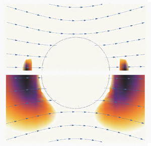
Let us examine where the suppression occurs around a particle moving in the way supposed in figure 1. In the approximation mentioned below (2.12), we use  $s^{(0)}$ instead of $s$ in (2.5) to calculate $|\tilde {\eta }^{(1)}/\tilde {\eta }^{(0)}|$ for $c=1$ and $U=\bar {U}$, and show the results in figure 5, where the suppression occurs in coloured regions. The maximum of (2.14) is taken at $(\rho , \theta )= (\sqrt {2}, 0)$ or $(\sqrt {2},{\rm \pi} )$. The value of $\vert \tilde {\eta }^{(1)}/\tilde {\eta }^{(0)}\vert$ equals $\kappa$ at these points, and becomes smaller at a point more distant from these points, as shown in figure 5. The maximum of ${\tau }_{s^{(0)}}$ is $0.0129\times c^{0.518}$ for $U=\bar {U}$, and is $0.0264\times c^{0.518}$ for $U=4\bar {U}$, which is approximately the effective cutoff in our numerical integration. The latter yields $\kappa \approx 0.13$ at $\tau =10^{-3}$ and $\approx 0.21$ at $\tau =10^{-4}$ for $c=1$ and $U=4\bar {U}$. Thus, $\kappa$ is adequately small as compared with unity in the range of $\tau$ examined in figure 3, which would make our formulation globally meaningful.

Figure 5. Colour gradation represents the largest of zero and  $1-\check {\tau }_{s^{(0)}}^{\nu (d-z)}$ for $c=1$ and $U=\bar {U}$ at each of $\tau =1.26\times 10^{-2}$ $(a)$ and $8.064\times 10^{-3}$ $(b)$. The particle is assumed to move translationally with the velocity $\bar {U}\boldsymbol {e}_z$. The region shown in each figure is the same as in figure 1; the dotted curve represents the half of the cross-section of the particle surface. The curves outside the particle are the stream lines of $\boldsymbol {v}^{(0)}$, which are represented by arrows in figure 1.
From the maximum of  ${\tau }_{s^{(0)}}$ for $U=\bar {U}$ mentioned above, $\kappa$ is found to become non-zero when $\tau$ is smaller than $1.29\times 10^{-2}$ for $c=1$ and $U=\bar {U}$. This value of $\tau$ approximately agrees with the onset temperature of the suppression estimated in Beysens (Reference Beysens2019), where the shear rate, with its inhomogeneity and dependence on $U$ being neglected, is evaluated to be a typical shear rate, $\bar {U}/r_0$. The value of $\tau$ is slightly smaller than $1.29\times 10^{-2}$ in figure 5(a), where a very weak suppression occurs in narrow regions around $(\rho , \theta )= (\sqrt {2}, 0)$ and $(\sqrt {2},{\rm \pi} )$ for $c=1$ and $U=\bar {U}$, as expected. However, at this temperature, the suppression cannot be read in figure 3. In figure 5(b) with smaller $\tau$, $|\tilde {\eta }^{(1)}/\tilde {\eta }^{(0)}|$ becomes larger in wider regions, which means that the suppression occurs more strongly and extensively, although the suppression can be read only slightly from the solid circle at this temperature and cannot be read from the open circle closest to this temperature in figure 3. It is for $\tau <3.2\times 10^{-3}$ in figure 3 that the suppression can be read explicitly from the experimental data ( $\circ$); the suppression for $c=1$ and $U=\bar {U}$ should occur more strongly and extensively in this range of $\tau$ than in figure 5(b). Thus, we overestimate the onset temperature of the suppression in the data of the self-diffusion coefficient if we evaluate the shear rate to be $\bar {U}/r_0$.
For  $U=4\bar {U}$, as mentioned above, the maximum of $\tau _{s^{(0)}}$ is $0.0264\times c^{0.518}$. The maximum is smaller than unity in the range of $c$ examined in figure 4, as supposed in our formulation. This also shows that our results are free from the details of a formal rule for large particle speed in appendix D. In the absence of the suppression, we have $\xi =\xi _0\tau ^{-\nu }=28\ \textrm {nm}$ and $120\ \textrm {nm}$ for $\tau =10^{-3}$ and $10^{-4}$, respectively. The correlation length should be reduced by the strong shear, which suppresses the order-parameter fluctuation with small wavenumber. The correlation length under the shear effect is dependent on the direction, and proportional to $\tau ^{-0.5}$ at the largest in the stagnation-point flow (Onuki & Kawasaki Reference Onuki and Kawasaki1980c). This exponent is the same as in the mean-field approximation. The curvature of the stream line in figure 3 suggests that a typical length of the flow is several times larger than the particle diameter. Thus, a typical length of the flow is sufficiently large as compared with $\xi$ in the range of $\tau$ examined in figure 3, as supposed in our formulation.
It is assumed in (2.4) that the suppression is perfect if it occurs. In terms of the renormalization-group calculation, the singular part of the viscosity changes in the coarse-graining procedure, which makes sense until the resolution reaches  $\xi$, and the way of the change is altered when the resolution exceeds a threshold determined by the shear rate. Equation (1.3) can be derived from the condition of whether the threshold comes before $\xi$ or not, as mentioned in the latter half of appendix A. In the procedure after the alteration, the singular part of the viscosity continues to be changed and becomes anisotropic. Thus, the assumption in (2.4) does not hold exactly. The ratio of the correction in the later stage, i.e. in the stage after the alteration, to the one in the earlier stage is evaluated by averaging the former correction over the directions in appendix E. If $d=3$ is substituted into these results valid up to the linear order with respect to $4-d$, the evaluated ratio is smaller than $4\ (7)$ per cent for a pure-extension flow (a simple shear flow). These small values would support the appropriateness of (2.4), which can explain the data for the three-dimensional mixture of Beysens (Reference Beysens2019) in figure 3.
In deriving (1.3), the lifetime of a correlated cluster and the range of the cluster size are evaluated. However, some deviations are possible in these evaluations, and may be required to compensate for the approximation in (2.4) mentioned above. For example, let us consider replacing  $\xi$ with $1.5 \xi$ in (1.3). This replacement is equivalent with putting $c$ equal to $1.5^{z}\approx 3.5$. A change of (1.3) to this extent cannot be denied from the data of Beysens (Reference Beysens2019) in figure 3, considering that the red short bars above the solid circles still lie in the middle of the distribution of the data.
We simply link the drag coefficient with the self-diffusion coefficient by means of the one-dimensional Langevin equation for the particle velocity. Similar nonlinear Langevin equations are used for different problems in Klimontovich (Reference Klimontovich1994) and Lindner (Reference Lindner2007). Validity of the Langevin equation with the Stratonovich interpretation in our problem, where the viscosity can be inhomogeneous and dependent on the particle speed, remains to be founded on the fluctuating hydrodynamics, unlike in the cases studied by Bedeaux & Mazur (Reference Bedeaux and Mazur1974) and Mazur & van der Zwan (Reference Mazur and van der Zwan1978). It still appears that the Langevin equation can describe the data of Beysens (Reference Beysens2019) well in figure 3, where a rather large distribution of the data for small  $\tau$ in the direction of the vertical axis may come from the properties of the viscosity in our problem.
4. Summary and concluding remarks
Correlated clusters of the order-parameter fluctuation are generated in a near-critical binary fluid mixture lying in the homogeneous phase near the demixing critical point. The upper size of clusters, the correlation length, becomes larger as the critical point is approached. Then, as is well known, the convection of large and long-lived clusters enhances the transport coefficients in the coarse-grained dynamics (Kawasaki Reference Kawasaki1970). It is also well known that a sufficiently strong shear, if imposed, can deform long-lived clusters to suppress the critical enhancement (Onuki & Kawasaki Reference Onuki and Kawasaki1979). In a recent experiment (Beysens Reference Beysens2019), shear around a Brownian particle in a near-critical mixture on the critical isochore was suggested to cause this suppression to influence the motion. Deviation of the self-diffusion coefficient from the Stokes–Sutherland–Einstein formula was observed in the temperature range where the suppression is judged to occur from a typical shear rate around a particle moving with a typical speed.
How the deviation depends on the temperature is calculated in the present study. We first calculate the drag coefficient of a particle moving translationally in a mixture which is quiescent far from the particle. The suppression is simply assumed to occur perfectly when the cluster with the size of the correlation length becomes so long-lived as to be deformed by the shear. The shear rate is inhomogeneous and depends on the particle speed. Hence, the suppression makes the viscosity inhomogeneous and dependent on the particle speed. The calculation supposes a low Reynolds-number and a sufficiently weak influence of the shear on the viscosity, which are realized in the experiment. We next employ the drag coefficient thus calculated, dependent on the particle speed, as the frictional coefficient in a one-dimensional Langevin equation of the Stratonovich type to calculate the self-diffusion coefficient. The calculation results agree well with the experimental data, which is rather robust to changes in the threshold for the occurrence of the suppression.
Acknowledgements
The author thanks S. Yabunaka for helpful discussions.
Declaration of interests
The author reports no conflict of interest.
Appendix A. Previous results of the renormalization-group calculations
For an equilibrium binary fluid mixture in the homogeneous phase on the critical isochore near the critical point, as the renormalization steps are iterated, the Onsager coefficient for the interdiffusion approaches a constant, denoted by  $\lambda ^*$. Rewinding the rescaling procedure to decrease the cutoff wavenumber $k$ at each iteration, we obtain the coefficient coarse grained up to $k$. Writing $\lambda$ for it, we have
 \begin{equation} \lambda=\lambda^* \left(\frac{k_{o}}{k}\right)^{4-\eta-z}\quad \textrm{if}\ k\xi \gtrsim 1 ,\end{equation}
that is, if  $k\xi$ is larger than or comparable to unity. Here, $k_{o}(\gg k)$ is the cutoff wavenumber before coarse graining and thus $1/k_{o}$ has a microscopic length. If $k\xi$ is much smaller than unity, $1/k$ in the parentheses of (A 1) should be replaced by $\xi$; rewinding the rescaling procedure makes sense up to the length scale of $\xi$. Likewise, the singular part of $\tilde {\eta }$ is given by $\tilde {\eta }^* (k_{o}/k)^{z-d}$ for $\xi ^{-1} \stackrel {<}{\sim } k\ll k_{o}$ and
 \begin{equation} \tilde{\eta}^* (k_{o}\xi)^{z-d} \quad\textrm{if}\ k\xi\ll 1 , \end{equation}
where  $\tilde {\eta }^*$ denotes a constant for $\tilde {\eta }$ corresponding with $\lambda ^*$ (Onuki & Kawasaki Reference Onuki and Kawasaki1979). These exponents can be also derived from the dynamic scaling assumption (Folk & Moser Reference Folk and Moser2006).
We define the order parameter so that the coefficient of the square-gradient term in the dimensionless effective Hamiltonian is a half, as in Siggia et al. (Reference Siggia, Hohenberg and Halperin1976), Onuki & Kawasaki (Reference Onuki and Kawasaki1979) and Onuki (Reference Onuki2002). In the Fourier transform mentioned above (1.1), we put the two times equal to each other and write  $\chi _k$ for the result, which is the static correlation function or static susceptibility. We have $\chi _k\approx \xi ^2(k/k_{o})^{\eta }$ for $k\xi \ll 1$. As $k\to 0$ and $\xi \to \infty$ with $k\xi$ being an arbitrary positive number, the renormalization-group calculation gives (Siggia et al. Reference Siggia, Hohenberg and Halperin1976)
 \begin{equation} \varGamma_k= \frac{Rk_{B}T_{c}}{\tilde{\eta}\xi^{d-2}}k^2\bar{\varOmega}(k\xi), \end{equation}
where the Kawasaki amplitude  $R$ is a universal constant approximately equal to $1/(6{\rm \pi} )$. The dimensionless scaling function, ${\bar \varOmega }$, tends to unity as its variable approaches zero. Considering that $\lambda \tilde {\eta } \xi ^{d-2}$ divided by $\chi _k$ equals $Rk_{B}T_{c}$ for $k\xi \ll 1$, we have
 \begin{equation} \frac{\varGamma_k}{k^2} \to \lambda^* k_{o}^{4-z} \xi^{2-z} \quad\textrm{as}\ k\to 0 \end{equation}
with  $k\xi$ being fixed to be small (Siggia et al. Reference Siggia, Hohenberg and Halperin1976).
According to the renormalization-group calculation up to the order of  $\epsilon \equiv 4-d$ in the presence of a simple shear flow (Onuki & Kawasaki Reference Onuki and Kawasaki1979), (A 1) is found to break down for $k\stackrel {<}{\sim }k_s$, where $k_s$ is defined so that
 \begin{equation} \lambda^*k_{o}^{4-z} k_s^z = {s} \end{equation}
holds. The shear is strong enough to suppress the critical enhancement if  $k_s\xi \gtrsim 1$ holds; $k_s$ then comes before $1/\xi$ in the coarse-graining process of decreasing $k$ (figure 6). Otherwise, $\lambda$ for $k\xi \ll 1$ remains given by (A 1) with $1/k$ being replaced by $\xi$. With the aid of (A 3)–(A 5), we find that this condition of strong shear approximately agrees with (1.3). From (2.3) and (A 5), we have $k_s^{-1}=\xi _0 \tau _s^{-\nu }$ and
 \begin{equation} s^*\equiv \lambda^*k_{o}^{4-z}\xi_0^{-z}. \end{equation}
Ambiguity on the condition of strong shear is discussed in § 3.

Figure 6. A schematic graph showing how  $\lambda$ changes as the mixture is coarse grained, which is made from figure 2 of Onuki & Kawasaki (Reference Onuki and Kawasaki1979). We define $k$ so that the cutoff wavenumber viewed on the original lattice equals $k$ at the iteration number, $l$, in the renormalization-group calculation. We have $k/k_{o}=\tilde{b}^{-l}$, where $\tilde{b}$ is the length rescaling factor. The curve follows (A 1) for $k_{o}\gg k \gg k_s$, but deviates from (A 1) for $k_s\gtrsim k$.
The above-mentioned breakdown of (A 1) occurs when the static susceptibility deviates from the Ornstein–Zernike form in the mean-field approximation for an equilibrium fluid mixture. Then, using the wavenumber vector  $\boldsymbol {k}$, we should write $\chi _{\boldsymbol {k}}$, not $\chi _k$, for the susceptibility because of its anisotropy. The method of characteristics is used to calculate $\chi _{\boldsymbol {k}}$ for a simple shear flow in § 3 of Onuki & Kawasaki (Reference Onuki and Kawasaki1979), and for other kinds of linear shear flow in § 4 of Onuki & Kawasaki (Reference Onuki and Kawasaki1980a) and § 3 of Onuki & Kawasaki (Reference Onuki and Kawasaki1980c). In this method, a wavenumber vector dependent on a parameter, with the dimension of the time, is introduced, and the ‘time’ derivative of the vector equals the product of the matrix of the velocity gradient and the vector. Thus, $s$ in (1.3) can be determined in the way described in § 1.
The renormalization correction of  $\lambda$ in the later stage with $k<k_s$ in a simple shear flow becomes dependent not only on $k$ but also on $\boldsymbol {k}$, and is much smaller than the one in the earlier stage with $k>k_s$ even when $\epsilon$ is put equal to unity, as shown by (4.62) and (4.85) of Onuki & Kawasaki (Reference Onuki and Kawasaki1979). We draw figure 6 from figure 2 of Onuki & Kawasaki (Reference Onuki and Kawasaki1979), where it is stated that the singular part of the viscosity behaves in the same fashion, although the viscosity for $k<k_s$ is not only dependent on $\boldsymbol {k}$ but also expressed in terms of an anisotropic tensor (Onuki & Kawasaki Reference Onuki and Kawasaki1980b). Within a simplified picture of figure 6, assuming (2.4) amounts to drawing the curve of the singular part of $\tilde {\eta }$ as if the curve for $k\ge k_s$ were perfectly free from the shear effect and linked to a horizontal line in $k<k_s$.
Appendix B. Local shear rate
We here examine how  $\boldsymbol {\nabla } \boldsymbol {v}^{(0)}$ changes around a particle, which is briefly mentioned above (2.14). From (2.8a–c), we can calculate the components of $\boldsymbol {\nabla } \boldsymbol {v}^{(0)}$ with respect to the three-dimensional Cartesian coordinates $(x,y,z)$ at a point on the $xz$ plane ( $\phi =0$). There, the $(x,y)$, $(y,x)$, $(y,z)$ and $(z,y)$ components vanish. The components can be expressed in terms of a $3\times 3$ matrix. We rewrite this matrix as the sum of two matrices; one is the diagonal matrix with the diagonal elements being
 \begin{equation} (\nabla_xv^{(0)}_x+\nabla_zv^{(0)}_z)/2,\quad \nabla_yv^{(0)}_y \quad \textrm{and}\quad (\nabla_xv^{(0)}_x+\nabla_zv^{(0)}_z)/2 \end{equation}
from the top. We rotate the  $(x,z)$ coordinates to have $(x',z')$ coordinates so that the diagonal elements of the other matrix of the two vanish at the point; the diagonal matrix mentioned above is not changed by this rotation. The components of the velocity gradient with respect to the coordinates $(x', y, z')$ are given by
 \begin{equation} \frac{U}{r_0} \left[\begin{pmatrix} -C/2 & 0 & 0 \\ 0 & C & 0 \\ 0 & 0 & -C/2 \end{pmatrix}+\begin{pmatrix} 0 & 0 & B-A \\ 0 & 0 & 0 \\ B+A & 0 & 0 \end{pmatrix}\right], \end{equation}
where we use  $A\equiv 3\sin {\theta }/(4\rho ^2)$. We define $C$ as $\nabla _yv^{(0)}_y= 3(\rho ^2-1)\cos {\theta }/(4\rho ^4)$, and define $B$ as $3/(8\rho ^4)$ multiplied by the square root of
 \begin{equation} [-2+2(5-3\rho^2)\cos^2{\theta}]^2\sin^2{\theta} +[3(\rho^2-1)+2(5-3\rho^2)\sin^2{\theta}]^2\cos^2{\theta}. \end{equation}
Thus,  $A$ and $B$ are non-negative. The first term in the square brackets of (B 2) represents a pure-extension flow.
We define  $\varOmega _{e}$ as $\sqrt {B^2-A^2}$, and have
 \begin{equation} \varOmega_{e}^2=\frac{9(\rho^2-1)}{128\rho^8}[5\rho^2-13+(13\rho^2-5)\cos{2\theta}], \end{equation}
which vanishes at  $\rho =1$. As mentioned in the fourth paragraph of § 1, the exponential of the product of (B 2) and the time $t$ works as the time evolution operator for a convected line segment. The long-wavelength fluctuations of the order parameter are suppressed in the stretching direction. The exponential equals
 \begin{equation} \begin{pmatrix} e^{-C\check{t}/2} \textrm{cosh}\varOmega_{e}\check{t} & 0 & \left(B-A\right) \varOmega_{e}^{-1} e^{-C\check{t}/2} \textrm{sinh}\varOmega_{e}\check{t}\\ 0 & e^{C\check{t}} & 0 \\ \left(B+A\right) \varOmega_{e}^{-1} e^{-C\check{t}/2} \textrm{sinh}\varOmega_{e}\check{t} & 0 & e^{-C\check{t}/2} \textrm{cosh}\varOmega_{e}\check{t}, \end{pmatrix}\end{equation}
where we use  $\check {t}\equiv t U/r_0$ and note that the matrices in the square brackets of (B 2) commute. In figure 7 with $\rho =1.5$, we have $A>B$, i.e. purely imaginary $\varOmega _{e}$, for $0.74<\theta <2.4$ approximately, and $C^2>\varOmega _{e}^2$ for $0.6 <\theta <2.5$ approximately. Although data are not shown, as $\rho$ increases above unity, the $\theta$ region with $A>B$ and the one with $C^2>\varOmega _{e}^2$ are narrower. We find that $A>B$ holds at $\theta ={\rm \pi} /2$ for any $\rho$ larger than unity and that $\varOmega _{e}=1.5|C|$ holds at $\theta =0$ and ${\rm \pi}$. As $\theta$ changes from $0$ or ${\rm \pi}$ to ${\rm \pi} /2$, $\varOmega _{e}^2$ decreases more rapidly than $C^2$, as shown in figure 7. The two-dimensional flow with $C=0$ is considered in Onuki & Kawasaki (Reference Onuki and Kawasaki1980c), where a rotational flow with $A>B$ is shown to be weak in suppressing the critical enhancement. For simplicity, we thus neglect the periodic deformation of a cluster in determining the local shear rate.

Figure 7. We plot  $\varOmega _{e}^2$ (solid curve) and $C^2$ (dashed curve) at $\rho =1.5$ against $\theta$.
We suppose  $U>0$ in this paragraph. In the components of (B 5), when $\varOmega _{e}$ is real, the largest stretching rate is $CU/r_0$ if $C>0$ and is $(2\varOmega _{e}-C)U/(2r_0)$ if $C<0$. When $\varOmega _{e}$ is imaginary, the largest stretching rate is $CU/r_0$ if $C>0$ and is $-CU/(2r_0)$ if $C<0$. These results agree with (2.14), considering that (2.14) with $c=1$ equals $|C{U}|{/r_0}$. We find for $U>0$ that $c$ is unity for $0\le \theta \le {\rm \pi}/2$, is $1/2$ for ${\rm \pi} /2< \theta \le {\rm \pi}$ and $\varOmega _{e}^2<0$, and increases up to $2$ as $\theta$ increases in the region of ${\rm \pi} /2< \theta \le {\rm \pi}$ and $\varOmega _{e}^2\ge 0$.
Appendix C. Some details in calculating the drag force
We introduce
 \begin{equation} \varGamma^{({com})}_J(\rho,\sigma)\equiv \frac{1}{4\rho^{J+2}\sigma^{J+2}}\left[ \frac{1}{2J+3}-\frac{\sigma^2}{2J+1}\right] +\frac{1}{4\rho^J\sigma^{J+2}}\left[ \frac{\sigma^2}{2J-1}-\frac{1}{2J+1}\right], \end{equation}
and the kernel appearing in (2.22) is given by
 \begin{equation} \varGamma_J(\rho,\sigma)\equiv \varGamma^{({com})}_J(\rho,\sigma)+ \frac{\sigma^{J-1}}{2\rho^{J+2} \left(2J+1\right)} \left[ \frac{\sigma^2}{2J+3}-\frac{\rho^2}{2J-1}\right] \quad\textrm{for}\ \rho>\sigma, \end{equation}
together with  $\varGamma _J(\rho ,\sigma )=\varGamma _J(\sigma ,\rho )$ for $\rho <\sigma$. The kernel above for $J=1$ is equal to $1/30$ multiplied by $\varGamma _{R}$ of Okamoto et al. (Reference Okamoto, Fujitani and Komura2013). Similar calculations are there in Fujitani (Reference Fujitani2018) and Yabunaka & Fujitani (Reference Yabunaka and Fujitani2020).
As mentioned above (2.23), we can delete  $\varPi _J$ and $T_J$ from the last two terms of (2.13). A similar procedure can be found in deriving (4.19) of Okamoto et al. (Reference Okamoto, Fujitani and Komura2013). By using
 \begin{equation} -\frac{1}{2}\int_0^{\rm \pi} d\theta \sin^2{\theta}\frac{\partial}{\partial\theta} Y_{J0}(\cos{\theta})= \int_0^{\rm \pi}\,\textrm{d}\theta \sin{\theta}\cos{\theta}Y_{J0}(\cos{\theta})=\frac{\delta_{J1}}{\sqrt{{\rm \pi} \left(2J+1\right)}}, \end{equation}
where  $\delta _{ij}$ implies the Kronecker delta, we find the surface integral of the last two term of (2.13) to be given by
 \begin{equation} -\frac{2\sqrt{3{\rm \pi}}}{3}\tilde{\eta}^{(0)} r_0\left(\frac{1}{2}\partial_{\rho}^3+2\partial_{\rho}^2\right)R_{1} -\frac{\sqrt{6{\rm \pi}}}{3}r_0^3 H_{1}(1). \end{equation}
Differentiating (2.5) with respect to  $\rho$ or $\theta$ yields a term having the derivative of the step function, i.e. the delta function. Noting that this term vanishes because of its prefactor, we find that the negative of the right-hand side of (2.12) can be rewritten as
 \begin{equation} \frac{3U\tilde{\eta}^{(0)}}{r_0^{2}}\boldsymbol{h}\varTheta(\check{\tau}_{s^{(0)}}-1). \end{equation}
Here, the vector  $\boldsymbol {h}$ dependent on $(\rho ,\theta )$ can be calculated by using (2.8a–c). Because (2.17) is equal to (C 5), we use the orthogonality of the vector spherical harmonics to calculate $F_1$ and $H_1$. For example, $H_1(\rho )$ is the integral of the inner product of vectors of (C 5) and $\boldsymbol {B}_{10}$ over the surface of the unit sphere. We thus find that $H_1(\rho )$ vanishes at $\rho =1$, where (2.14), and thus $\check {\tau }_{s^{(0)}}$ vanish.
Substituting (2.8a–c) into the right-hand side of (2.12) and defining  $\zeta$ as $(d/z)-1$, we find that the components of $\boldsymbol {h}$ are given by
 \begin{equation} \left. \begin{gathered} h_r(\rho,\theta)=\left\{ \frac{1-\check{\tau}_s^{\nu(d-z)}}{\rho^3}+\zeta \check{\tau}^{\nu(d-z)} \left[ \frac{1-\rho^2}{\rho^4 s}\frac{\partial s}{\partial \rho}+\frac{1}{2\rho^5 s} \frac{\partial s}{\partial\theta}\tan{\theta}\right]\right\} \cos{\theta},\\ h_{\theta}(\rho,\theta)=\left\{ \frac{1-\check{\tau}_s^{\nu(d-z)}}{2\rho^3} +\zeta \check{\tau}^{\nu(d-z)}\left[ \frac{1}{2\rho^4 s}\frac{\partial s}{\partial \rho}+\frac{\rho^2-1}{2\rho^5 s} \frac{\partial s}{\partial\theta}{\cot}{\theta}\right]\right\}\sin{\theta}, \end{gathered} \right\} \end{equation}
and  $h_{\phi }=0$, where we write $s$ for $s^{(0)}$ for conciseness. We have $h_r(\rho ,\theta )=-h_r(\rho ,{\rm \pi} -\theta )$ and $h_{\theta }(\rho ,\theta )= h_{\theta }(\rho ,{\rm \pi} -\theta )$. From (2.20) for $J=1$, we obtain
 \begin{equation} \check{X}(\rho)=-\frac{\rho^2}{2} \int_0^{{\rm \pi}/2}\,\textrm{d}\theta [2 \sin{\theta}\cos{\theta} h_r(\rho,\theta)+\sin^2{\theta} \partial_{\rho} \rho h_{\theta}(\rho,\theta)]\varTheta(\check{\tau}_{s^{(0)}} -1), \end{equation}
where  $\partial _{\rho }$ operates on all the following terms including the step function.
Substituting (C 7) into (2.24), we employ integration by parts with respect to  $\rho$, and the resultant integrand contains the step function, not its derivative. Writing $\check {U}_c$ for ${c}|U|/U^*$, we have
 \begin{equation} \check{\tau}_{s^{(0)}}(\rho, \theta)=\frac{1}{\tau} \left[\frac{3\left(\rho^2-1\right)}{4\rho^4} \check{U}_c\cos{\theta}\right]^{1/(\nu z)} \end{equation}
in (C 7). Thus, the step function in (C 7) can be non-zero if
 \begin{equation} 4\rho^4-3\tau^{-\nu z}\check{U}_c(\rho^2-1)\cos{\theta}<0, \end{equation}
whose left-hand side is quadratic with respect to  $\rho ^2$. Putting the left-hand side above equal to zero gives $\rho =\rho _{\pm }$ and $\rho =-\rho _{\pm }$, where $\rho _{\pm }$ is defined as
 \begin{equation} \rho_{\pm}(\theta)\equiv \left(\frac{3\check{U}_c}{8\tau^{\nu z}}\cos{\theta}\pm\frac{\sqrt{\varDelta(\theta)}}{2}\right)^{1/2}. \end{equation}
Here,  $\varDelta$ is the discriminant, given by
 \begin{equation} \varDelta(\theta)\equiv \frac{3\check{U}_c}{\tau^{\nu z}} \left( \frac{3\check{U}_c}{16\tau^{\nu z}}\cos{\theta}-1\right)\cos{\theta} . \end{equation}
Equation (2.24) does not vanish if  $\varDelta$ is positive and if $\rho _-<\rho <\rho _+$, where we have $1<\rho _-<\rho _+$ for $\varDelta >0$.
We introduce
 \begin{equation} G_{m,n}(\theta)\equiv \varTheta(\varDelta(\theta))\int_{\rho_-(\theta)}^{\rho_+(\theta)}\,\textrm{d}\rho \left(\frac{\rho^2-1}{\rho^4}\right)^{\zeta-m} \frac{1}{\rho^n}, \end{equation}
which is expressed in terms of Gauss’ hypergeometric function according to Mathematica (Wolfram Research). The integral of (2.24) is found to be the sum of the integrals of the following three integrands over  $0<\theta <{\rm \pi} /2$. The integrands are
 \begin{equation} \varTheta(\varDelta(\theta))\int_{\rho_-(\theta)}^{\rho_+(\theta)}\,\textrm{d}\rho\ \left(\frac{3\rho^2+1}{4\rho^4}\sin^3{\theta}+\frac{1-3\rho^2}{\rho^4}\sin{\theta}\cos^2{\theta}\right), \end{equation}
where the integration with respect to  $\rho$ is elementary,
 \begin{equation} -\left(\frac{3\check{U}_c}{4\tau^{\nu z}}\right)^{\zeta} \frac{1}{4}\left[3G_{0, 2}+G_{0, 4}+\zeta\left(3 G_{1,4}-5 G_{1,6}-G_{1,8}-5G_{1,10}\right)\right] \cos^{\zeta}{\theta}\sin^3{\theta} \end{equation}
and
 \begin{equation} \left(\frac{3\check{U}_c}{4\tau^{\nu z}}\right)^{\zeta} \left[3G_{0,2}-G_{0,4}-\zeta\left( 6G_{0,2}-14G_{0,4}+4G_{0,6}\right)\right] \cos^{\zeta+2}{\theta}\sin{\theta}, \end{equation}
where the variable  $\theta$ of $G_{m, n}$ is dropped for conciseness.
Appendix D. Self-diffusion coefficient
The Fokker–Planck equation corresponding to (2.26) is
 \begin{equation} \frac{\partial}{\partial t} P(U,t;U_0)=\frac{1}{m}\frac{\partial}{\partial U} \left(\gamma U P\right) +\frac{1}{2m^2}\frac{\partial}{\partial U}b\frac{\partial}{\partial U}bP, \end{equation}
where  $P(U,t;U_0)$ represents the probability density of $U$ at a time $t$ on condition that $U=U_0$ at $t=0$. The variables of the functions are dropped on the right-hand side above for conciseness. The stationary solution, denoted by $P_{eq}(U)$, is proportional to (Risken Reference Risken2002)
 \begin{equation} \frac{m^2}{b^2}\exp{\left[ \int\,\textrm{d}U \left(\frac{1}{2b^2}\frac{\textrm{d}b^2}{\textrm{d}U}-\frac{2m\gamma U}{b^2}\right)\right]}, \end{equation}
which should be proportional to the Boltzmann distribution (Zwanzig & Bixon Reference Zwanzig and Bixon1975),
 \begin{equation} \sqrt{\frac{m}{2{\rm \pi} k_{B}T}} e^{-mU^2/(2k_BT)} . \end{equation}
Considering that  $b^2$ equals $2\gamma k_{B}T$ if $\gamma (U)$ is independent of $U$, we find
 \begin{equation} b(U)^2=4m e^{mU^2/(k_{B}T)}\int_U^{\infty}\,\textrm{d}U_1\ \gamma(U_1)U_1\textrm{e}^{-mU_1^2/(k_{B}T)}. \end{equation}
We can rewrite the right-hand side above by changing the integration interval to the one from  $U$ to $-\infty$ because the integral from $-\infty$ to $\infty$ vanishes. Then, using integration by parts, we find that $|b(U)^2-2k_{B}T \gamma (U)|$ equals
 \begin{equation} 2k_{B}T e^{mU^2/(k_{B}T)}\left|\int_{-U}^{\infty}\,\textrm{d}U_1\ \gamma'(U_1)\textrm{e}^{-mU_1^2/(k_{B}T)}\right|, \end{equation}
where the prime indicates the derivative. We can assume that  $\check {\gamma }(u)$ decreases to a positive constant as $|u|$ increases to $\infty$ for the reason mentioned in the next paragraph. Thus, for $U<0$, (D 5) becomes larger if we replace $\gamma '(U_1)$ with a suitable positive constant. Using an asymptotic form of a complementary error function, we find that (D 5) vanishes, and thus $b(U)^2$ remains finite, in the limit of $U\to -\infty$. This result is used later.
We can make a convenient formal rule for the particle speed larger than assumed in the text, because we later find its influence on (2.28) negligible. In other words, making such a rule is a substitute for introducing an upper cutoff of the particle speed to the model in the text. For definiteness, we here specify a formal rule. In (2.1), we should replace  $\tau$ with unity for $\tau >1$. Accordingly, (2.4) is supplemented with the rule $\tilde {\eta }=\tilde {\eta }_{B}(T)$ for $\tau >1$ if $\tau _s<1$ and for any $\tau$ otherwise. As the particle speed is larger, because the region with $\tau _s>1$ approaches the whole mixture region, ${\gamma }(U)$ approaches Stokes’ law of $6{\rm \pi} \tilde {\eta }_{B}(T) r_0$ from the larger side. This means that $\check {\gamma }(\infty )$ is not smaller than $\tau ^{\nu (z-d)}$, which is $0.75$ and $0.68$ for $\tau =10^{-3}$ and $10^{-4}$, respectively. Thus, the assumption mentioned in the preceding paragraph holds in the range of $\tau$ of figure 3.
Introducing a Laplace transform, defined as
 \begin{equation} \hat{Q}(U, \sigma; U_0)\equiv \int_0^{\infty}\,\textrm{d}t\left[P(U,t;U_0)-P_{eq}(U)\right]e^{-\sigma t}, \end{equation}
we use  $\langle U_0 \rangle =0$ to rewrite (2.27) as
 \begin{equation} D=\int_{-\infty}^{\infty}\,\textrm{d}U \int_{-\infty}^{\infty}\,\textrm{d}U_0\ UU_0 \hat{Q}(U, 0; U_0)P_{eq}(U_0) . \end{equation}
From the Laplace transform of (D 1), we use (D 2) and (D 3) to obtain
 \begin{equation} -\delta(U-U_0)+P_{eq}(U)=\frac{1}{2m^2}\frac{\partial}{\partial U} b^2(U)P_{eq}(U) \frac{\partial}{\partial U}\frac{\hat{Q}(U,0; U_0)}{P_{eq}(U) } , \end{equation}
where  $\delta$ represents the delta function. With $\mathcal {O}$ indicating the Landau symbol, we have $\hat {Q}(U, \sigma; U_0)<\mathcal {O}(|U|^{-1})$ as $| U|\to \infty$ because the normalization conditions of $P$ and $P_{eq}$ give
 \begin{equation} \int_{-\infty}^{\infty}\,\textrm{d}U\ \hat{Q}(U, \sigma; U_0)=0 . \end{equation}
As mentioned above,  $b(U)^2$ remains finite in the limit of $U=-\infty$. Integrating (D 8) with respect to $U$ from $-\infty$ gives
 \begin{equation} \frac{2m^2}{b^2(U)P_{eq}(U)}\left[-\varTheta(U-U_0)+\int_{-\infty}^U\,\textrm{d}U_1\ P_{eq}(U_1)\right] = \frac{\partial}{\partial U}\frac{\hat{Q}(U,0;U_0)}{P_{eq}(U) }. \end{equation}
Integrating (D 10) with respect to  $U$ from a value smaller than $U_0$, substituting the result into (D 7) and using $\langle U_0 \rangle =0$, we arrive at
 \begin{equation} D=-2m^2 \int_{-\infty}^{\infty}\,\textrm{d}U\ \int_{-\infty}^{\infty}\,\textrm{d}U_0\ UU_0P_{eq}(U)P_{eq}(U_0)\int_{U_0}^U\,\textrm{d}U_1\ \frac{1}{b(U_1)^2P_{eq}(U_1)}. \end{equation}
Interchanging the order of the integrals above, we use  $\check {\gamma }(u)=\check {\gamma }(-u)$ to obtain (2.28).
Some details on numerical calculations of (2.28) are mentioned below. We define  $L$ as
 \begin{equation} L(u_{a}, u_{b})=\int_{u_{a}}^{u_{b}}\,\textrm{d}u_1\ \check{\gamma}(u_1)u_1 e^{-Mu_1^2} . \end{equation}
We can choose  $u_{c}(>0)$ so that $|\check {\gamma }'(u)|$ is smaller than $|\check {\gamma }'(u_{c})|$ for $u>u_{c}$. The integral in the square brackets of (2.28) is given by $L(u, \infty )$. Using integration by parts, we obtain
 \begin{equation} L(u_{c},\infty)=\frac{\check{\gamma}(u_{c})}{2M}e^{-Mu_{c}^2}\left[1+ \frac{\textrm{e}^{Mu_{c}^2}}{\check{\gamma}(u_{c})} \int_{u_{c}}^{\infty} \,\textrm{d}u_1\ \check{\gamma}'(u_1) \textrm{e}^{-Mu_1^2}\right]. \end{equation}
The absolute value of the second term in the square brackets above is smaller than
 \begin{equation} \frac{\left|\check{\gamma}'(u_{c})\right|{e}^{Mu_{c}^2}}{\check{\gamma}(u_{c})\sqrt{M}}\int_{u_{c}\sqrt{M}}^{\infty} \textrm{d}x\ e^{-x^2} \approx \frac{\left| \check{\gamma}'(u_{c})\right|}{2Mu_{c}\check{\gamma}(u_{c})}, \end{equation}
where the approximation is good for  $u_{c}\sqrt {M}\gtrsim 1$. In our numerical calculations, we choose $u_{c}$ so that $u_{c}\sqrt {M}\approx 4$, and find that the right-hand side above is smaller than $10^{-3}$, which enables us to neglect the second term in the square brackets of (D 13).
The integral with respect to  $u$ in (2.28) is rewritten as
 \begin{equation} \int_{0}^{u_{c}}\,\textrm{d}u\ \frac{e^{-3Mu^2/2}}{L(u,\infty)} +\int_{u_{c}}^{\infty}\,\textrm{d}u \frac{e^{-3Mu^2/2}}{L(u,\infty)} , \end{equation}
where  $u_{c}$ is chosen as indicated above. In the first term above, we can use
 \begin{equation} L(u, \infty)\approx L(u, u_{c}) +\frac{{\tilde \gamma}({u_{c}})}{2M}e^{-Mu_{c}^2}. \end{equation}
In the second term of (D 15), because of  $u>u_{c}$, $L(u,\infty )$ can be approximated to be the second term on the right-hand side of (D 16) with $u_{c}$ being replaced by $u$ for the same reason as described in the preceding paragraph. Thus, the second term of (D 15) is approximately equal to
 \begin{equation} \frac{2M}{\check{\gamma}(u_{c})}\int_{u_{c}}^{\infty}\,\textrm{d}u\ e^{-Mu^2/2}. \end{equation}
Here, we use  $\check {\gamma }(u_{c})\approx \check {\gamma }(\infty )$. In our numerical calculation, with $u_{c}$ being chosen as indicated above, the ratio of (D 17) to the first term of (D 15) is much smaller than $10^{-3}$, and thus the first term is regarded as equal to the integral with respect to $u$ in (2.28). Hence, we can calculate (2.28) by using $\check {\gamma }(u)$ with $u\le u_{c}$, or in other words, by using $\gamma (U)$ with $U$ smaller than $4\bar {U}$ approximately. Thanks to this effective cutoff speed, our calculation results are free from the details of the rule for a large particle speed, as checked quantitatively in § 3.
Appendix E. Renormalization correction under the shear effect
A simple shear flow in four dimensions is used in the calculation mentioned above (A 5). The components of its velocity gradient with respect to the Cartesian coordinates vanish except for  $\nabla _2v_1$, which is a positive constant. As mentioned at the end of appendix A, the singular part of the viscosity changes as $k$ decreases from $k_{o}$. The ratio of the change in the later stage with $k<k_{s}$, to the change in the earlier stage with $k>k_{s},$ is given by the second term in the square brackets of (4.64) of Onuki & Kawasaki (Reference Onuki and Kawasaki1979). To evaluate this ratio, we take average of the term over the orthogonal components and average over the directions of the wavenumber vector. The former average is obtained by dividing (4.65) of Onuki & Kawasaki (Reference Onuki and Kawasaki1979) by three – the dimension of the divergence-free space. In this equation, the dot immediately after the fraction should be deleted to validate the equality, and the right-hand side, as it is, represents the trace of the left-hand side. The latter average is obtained by replacing $\hat {\boldsymbol {k}}$ in (4.65) of Onuki & Kawasaki (Reference Onuki and Kawasaki1979) by one of the four orthogonal unit vectors, summing the results over the four vectors, and dividing the sum by the spatial dimension, four. The result derived from theses averages is denoted by $\delta _{s}$. As in deriving the right-hand side of (3.6) of Onuki & Kawasaki (Reference Onuki and Kawasaki1979), we use the method of characteristics to find $\delta _{s}$ to be given by $4\epsilon /(19{\rm \pi} ^2)$ multiplied by the integral of
 \begin{equation} \frac{2}{q_1}(q_1^2q_3^2+q_1^2q_4^2+q_3^2q_4^2) I(\boldsymbol{q}) \end{equation}
with respect to the four-dimensional vector  $\boldsymbol {q}$ over half the unit sphere with $q_1>0$, where $I(\boldsymbol {q})$ is defined as the integral of the following integrand over $p$ running from $q_2$ to $\infty$. The integrand is given by
 \begin{equation} \exp{\left[ \frac{2}{3 q_1}\left\{ \frac{3}{5}( q_2^5-p^5) +(q_1^2+q_3^2+q_4^2) [2(q_2^3-p^3)+3(q_2-p)] \right\}\right]} \end{equation}
divided by  $(0.97 \vert q_1\vert ^{2/5} +q_1^2+p^2+q_3^2+q_4^2)^2$. If we replace this denominator by $q^4$, where $q$ denotes $|\boldsymbol {q}|$, (E 1) becomes larger. Putting $q_3=q_4=0$ and changing the variable $p$ to $Z\equiv 2(p-q_2)/q_1$ in (E 2), we obtain a new exponential function. Its integral over $0<Z<\infty$ is denoted by $I_1(q_1,q_2)$, and we have
 \begin{equation} \delta_{s}<\frac{4\epsilon}{19{\rm \pi}^2} \int\,\textrm{d}\boldsymbol{q} \frac{q_1^2q_3^2+q_1^2q_4^2+q_3^2q_4^2}{q^4}I_1(q_1,q_2), \end{equation}
where the integral is taken over half the unit sphere mentioned above. In the square brackets of (E 2) after the above-mentioned conversion, the leading term for large  $Z$ is given by $-q_1^4Z^5/80$. Thus, as $q_1$ approaches zero from the positive side, the leading term of $I_1(q_1,q_2)$ is proportional to $q_1^{-4/5}$, which justifies that we neglected the contribution from the integrand with $q_1=0$ to the integral of (E 1). This integral shows $\delta _{s}>0$.
Introducing the polar coordinates of  $\boldsymbol {q}$, we can numerically perform the integral of (E 3) over the angular components. We write $J(q,Z)$ for the result, and have
 \begin{equation} \delta_{s}<\frac{4\epsilon}{19{\rm \pi}^2} \int_0^1\,\textrm{d}q \int_0^{\infty}\,\textrm{d}Z \ J(q,Z). \end{equation}
If we retain only the leading term in (E 2),  $J(q,Z)$ in (E 4) is replaced by
 \begin{equation} J_1(q,Z)\equiv \frac{2{\rm \pi} q^3}{15} \int_0^{{\rm \pi}/2}\,\textrm{d}\theta_1\ e^{-q_1^4Z^5/80} (20-18\sin^2{\theta_1})\sin^4{\theta_1}, \end{equation}
where  $\theta _1$ is defined so that $q_1=q\cos {\theta _1}$ holds. The integral in (E 5) can be expressed in terms of generalized hypergeometric functions, and the integral of $J_1(q,Z)$ over $0<Z<\infty$ turns out to be proportional to $q^{11/5}$, according to Mathematica (Wolfram Research). Numerically, $J(q,Z)$ is shown in figure 8 to be smaller than $J_1(q,Z)$. The double integral in (E 4) with $J$ replaced by $J_1$ equals $3.44$, which leads to $0<\delta _{s}<7.33\times 10^{-2}\epsilon$.

Figure 8. From the top, three solid curves, respectively, represent  $J_1(1.0,Z), J_1(0.5,Z)$ and $J_1(0.05,Z)$, while three series of circles, respectively, represent $J(1.0,Z), J(0.5,Z)$ and $J(0.05,Z)$. We calculate $J(q,Z)$ by means of numerical integration in Mathematica (Wolfram Research) with Method $\to \{$‘GlobalAdaptive’, ‘MaxErrorIncreases’ $\to 10\,000$, Method $\to$ ‘GaussKronrodRule’ $\}$, MaxRecursion $\to 20$.
In a pure-extension flow in four dimensions, the off-diagonal elements of the velocity gradient vanish and  $\nabla _1 v_1=-3\nabla _2v_2=-3\nabla _3v_3=-3\nabla _4v_4$ is a positive constant. For this flow, we below evaluate the ratio of the changes in the later and earlier stages by taking averages in the same way as mentioned above, and write $\delta _{e}$ for the result corresponding with $\delta _{s}$. The ratio should be given by (4.65) of Onuki & Kawasaki (Reference Onuki and Kawasaki1979) with the denominator being replaced by $q^4-(q_1/2)\partial _{q_1}+(q_2/6)\partial _{q_2}+ (q_3/6)\partial _{q_3}+ (q_4/6)\partial _{q_4}$ and with the expression of the normalized susceptibility, denoted by $\chi ^*(\boldsymbol {q})$, being replaced by the one for the flow considered here. With the aid of (3.4) of Onuki & Kawasaki (Reference Onuki and Kawasaki1980a), $\chi ^*(\boldsymbol {q})$ is approximated to be $\sqrt {{\rm \pi} /2}$ for $q_1\ne 0$ in the pure-extension flow, as is consistent with (3.23b) of Onuki & Kawasaki (Reference Onuki and Kawasaki1980c). Thus, we find $\delta _{e}$ to be given by $4\epsilon /(19{\rm \pi} ^2)$ multiplied by the double integral of the following integrand over the unit sphere of the four-dimensional vector $\boldsymbol {q}$ and over ${w}=0$ to $\infty$. With $q_{\perp }^2$ denoting $q^2-q_1^2\equiv q^2\sin ^2{\theta _1}$, the integrand is the product of
 \begin{equation} \exp{\left[ \frac{q_1^4}{2}(1-e^{4{w}})+3q_1^2q_{\perp}^2(1-\textrm{e}^{4{w}/3}) +\frac{3q_{\perp}^4}{2}(e^{-4{w}/3}-1) \right]}, \end{equation}
which is larger if we delete the last two terms in the square brackets, and
 \begin{equation} \frac{\rm \pi}{4}\left[e^{2{w}/3}q_1^2q_{\perp}^2+\textrm{e}^{-2{w}/3}(q_2^2q_3^2+q_2^2q_4^2+q_3^2q_4^2)\right], \end{equation}
which is larger if we replace  $e^{-2{w}/3}$ with $e^{2{w}/3}$ in the second term in the square brackets. This expression shows $\delta _{e}>0$. Using a new variable $\zeta _1\equiv e^{2{w}/3}$, and performing the integration with respect to the angular components of $\boldsymbol {q}$ other than $\theta _1$, we have
 \begin{equation} \delta_{e}< \frac{4\epsilon}{19{\rm \pi}^2}\times \frac{3{\rm \pi}^2}{10}\int_0^1\,\textrm{d}q\ q^7 \int_0^{\rm \pi} \,\textrm{d}\theta_1 \ I_3(q,\theta_1)(5-4\sin^2{\theta_1})\sin^4{\theta_1}. \end{equation}
Here,  $I_3(q,\theta _1)$ is defined as the integral of $\exp {[-q^4(\zeta _1^6-1) (\cos ^4{\theta _1})/2]}$ over $\zeta _1=1$ to $\infty$. This integral is written in terms of the generalized exponential integral function, while the integration with respect to $\theta _1$ in (E 8) yields an expression involving generalized hypergeometric functions, according to Mathematica (Wolfram Research). Here, we note that $q^7I_3(q,\theta _1)$ tends to $0$ as $q$ approaches zero, and that $I_3(q,\theta _1)$ diverges, more slowly than $1/\vert \theta _1-{\rm \pi} /2\vert$, as $\theta _1$ approaches ${\rm \pi} /2$. We thus have $0<\delta _{e}<4.00\times 10^{-2}\epsilon$.


 Open access