


1. Introduction
Underwater propulsion is an area of research that brings together engineers and biologists alike; it has fostered a deeper understanding of aquatic locomotion and inspired innovation in underwater systems. The kinematics has the most significant effect on the locomotive properties of marine animals (Lighthill Reference Lighthill1960, Reference Lighthill1971; Triantafyllou, Triantafyllou & Gopalkrishnan Reference Triantafyllou, Triantafyllou and Gopalkrishnan1991; Triantafyllou, Triantafyllou & Grosenbaugh Reference Triantafyllou, Triantafyllou and Grosenbaugh1993; Borazjani & Sotiropoulos Reference Borazjani and Sotiropoulos2008; Eloy Reference Eloy2012; Saadat et al. Reference Saadat, Fish, Domel, Di Santo, Lauder and Haj-Hariri2017; Di Santo et al. Reference Di Santo, Goerig, Wainwright, Akanyeti, Liao, Castro-Santos and Lauder2021); however, some intricacies of animal evolution, such as the skins of sharks and odontocetes, have sparked research into the benefits of aquatic surface textures. Understanding the fluid dynamic interaction between kinematics and surface textures will help us to elucidate the contribution of surface textures to aquatic locomotion.
Previous work has identified important non-dimensional kinematic parameters for efficient swimming. The Reynolds number ( $Re$) affects the efficiency of swimmers, which can be in the viscous ( $Re \approx 10^2$), transitional ( $Re \approx 10^3$) and inertial ( $Re \to \infty$) regime (Borazjani & Sotiropoulos Reference Borazjani and Sotiropoulos2008, Reference Borazjani and Sotiropoulos2010). In this study, we focus on the transitional regime with $Re=[6, 24]\times 10^3$. The Strouhal number ( $St$) describes the ratio between the product of the wake width and the shedding frequency, and the flow velocity; Triantafyllou et al. (Reference Triantafyllou, Triantafyllou and Gopalkrishnan1991, Reference Triantafyllou, Triantafyllou and Grosenbaugh1993) found that the optimal Strouhal number should be in the range 0.25–0.35. Eloy (Reference Eloy2012) tested the kinematics of 53 different types of fish based on Lighthill's elongated body theory (Lighthill Reference Lighthill1960, Reference Lighthill1971), and found that for thin tails, the optimal Strouhal number range was 0.2–0.4. Saadat et al. (Reference Saadat, Fish, Domel, Di Santo, Lauder and Haj-Hariri2017) showed that the Strouhal number was insufficient for efficient locomotion, and defined a range of optimum motion amplitude to length ratio from $0.05$ to $0.15$. Di Santo et al. (Reference Di Santo, Goerig, Wainwright, Akanyeti, Liao, Castro-Santos and Lauder2021) recently compared 44 species of fishes and found that despite fishes’ different morphologies – categorised as anguilliform, subcarangiform, carangiform and thunniform – they shared a statistically significant oscillation amplitude, a.k.a. kinematic envelope. This work is noteworthy as previous work suggested that the presence of different kinematics was dependent on the morphology.
While kinematics has received the majority of the literature's attention, it is not the only factor affecting the locomotive properties of swimmers. Many studies have identified drag-reducing properties of certain textures. Although most of these studies are applied on static geometries, it has been suggested that these effects could transfer to unsteady aquatic propulsion. Bechert, Bruse & Hage (Reference Bechert, Bruse and Hage2000) showed that when shark-skin-like denticles interlock, they can passively reduce the drag on the surface much like a riblet. Riblets are small-scale two-dimensional transverse grooves whose heights scale with the viscous scales of the flow, and can act as drag reduction devices (Walsh Reference Walsh1982; Park & Wallace Reference Park and Wallace1994; García-Mayoral and Jiménez Reference García-Mayoral and Jiménez2011; Cui et al. Reference Cui, Pan, Wu, Ye and Wang2019). However, if riblets are not viscous scaled and/or have other larger-scale features (such as a larger pattern of inclinations), then they create new flow features and perhaps increase drag (Bechert et al. Reference Bechert, Bruse and Hage2000; Nugroho, Hutchins & Monty Reference Nugroho, Hutchins and Monty2013; Boomsma & Sotiropoulos Reference Boomsma and Sotiropoulos2016; Rouhi et al. Reference Rouhi, Endrikat, Modesti, Sandberg, Oda, Tanimoto, Hutchins and Chung2022; Von Deyn et al. Reference Von Deyn, Gatti, Frohnapfel, Von Deyn, Gatti and Frohnapfel2022). The sensitivity of riblets to these specific flow conditions calls into question their applicability to boost the performance of unsteady swimmers.
During a swim cycle, the surface of a swimmer might briefly encounter the viscous scales set out by Bechert et al. (Reference Bechert, Bruse and Hage2000) for drag-reduction of riblets; however, the morphing of the body and the fluctuating viscous length scales force the near-wall flow outside the conditions that cause riblets to decrease drag the majority of the time. To comprehend the potential hydrodynamic benefit of surface textures, we must look at them in the context of a larger, dynamic system. For example, vortex generators are often low-profile roughness elements that can significantly effect the flow and stimulate massive increases of aerodynamic performance when positioned correctly (Lin et al. Reference Lin, Robinson, McGhee and Valarezo1994; Lin Reference Lin2002). Similarly, studies suggest that shark skin uses passive control in the flank region to bristle the skin while swimming, increasing boundary layer mixing and helping to keep the flow attached at areas of flow reversal (Lang et al. Reference Lang, Motta, Hidalgo and Westcott2008; Afroz et al. Reference Afroz, Lang, Habegger, Motta and Hueter2016; Santos et al. Reference Santos2021). In this vein, Oeffner & Lauder (Reference Oeffner and Lauder2012) tested samples of skin from the midsection of a short-fin mako shark on both a rigid flapping plate and a flexible plate. They found that the skin actually reduced the rigid plate's propulsive effectiveness. They also found that adding shark skin increased the flexible plate's swimming speed by  $12\,\%$. However, they do not provide the amplitude envelope for the flexible plate that would ensure constant kinematics between the cases tested. Similarly, Wen, Weaver & Lauder (Reference Wen, Weaver and Lauder2014) covered an undulating plate in three-dimensional printed denticles of $100\times$ actual size, and measured a $6.6\,\%$ efficiency increase. Again, they do not provide an amplitude envelope to ensure that the kinematics between the smooth and the rough surfaces remains constant. The denticles in the above-mentioned work (Oeffner & Lauder Reference Oeffner and Lauder2012; Wen et al. Reference Wen, Weaver and Lauder2014) are not scaled with local viscous scales, so they are within the drag-reducing regimes set out by Bechert et al. (Reference Bechert, Bruse and Hage2000). Therefore, the physical mechanisms responsible for the differences between rough and smooth surfaces remain unclear and illustrate the need for a systematic study to examine the interaction between surface textures and kinematics.
The complex and multiscale shape of denticles does not lend itself to systematic investigations into the interplay between surface textures and kinematics. Consequently, we look to simplify the surface texture and focus on the first mode effects of roughness. We need to span a relevant physical space, yet ensure that the parametrisation of the surface is suited for the proposed problem. We look for inspiration in the surface textures/geometries that have been explored in previous studies that have focused on developing methods for predicting drag on flow over rough surfaces (Moody Reference Moody1944; Jiménez Reference Jiménez2004; Flack & Schultz Reference Flack and Schultz2010, Reference Flack and Schultz2014; García-Mayoral, Gómez-De-Segura & Fairhall Reference García-Mayoral, Gómez-De-Segura and Fairhall2019; Chung et al. Reference Chung, Hutchins, Schultz and Flack2021). Previous studies have indicated that the ratio of the total projected frontal roughness area to the wall-paralleled projected area (solidity,  $\varLambda$; Schlichting Reference Schlichting1936) and the mean slope of the roughness texture (in the streamwise and spanwise directions, also known as effective slope, $ES$; Napoli, Armenio & De Marchis Reference Napoli, Armenio and De Marchis2008) are two geometric parameters of a rough surface known to significantly affect the flow and forces. These two parameters can be altered easily for structured surfaces where the surface geometry has a sinusoidal shape. In fact, previous works have used sinusoidal roughness where the variation of the two roughness properties can be achieved by altering only the wavelength of the sinusoidal shape (Napoli et al. Reference Napoli, Armenio and De Marchis2008; Chan et al. Reference Chan, Macdonald, Chung, Hutchins and Ooi2015; Ma et al. Reference Ma, Xu, Sung and Huang2020; Ganju, Bailey & Brehm Reference Ganju, Bailey and Brehm2022). This presents us with a surface that can be used to understand how the primary scales of roughness (parametrised by a single quantity) interact with kinematics, with the hope that the findings can be generalised to more complex geometries.
In this work, we study the interaction between kinematics and roughness topologies through high-resolution simulations of a rough self-propelled swimming thin plate. We consider three Reynolds numbers ( $Re=6$, $12$ and $24\times 10^3$) with a focus on $Re=12\,000$ (based on swimming speed and chord length) to access moderate Reynolds numbers for the types of flows that are in line with previous efforts (Oeffner & Lauder Reference Oeffner and Lauder2012; Wen et al. Reference Wen, Weaver and Lauder2014; Saadat et al. Reference Saadat, Fish, Domel, Di Santo, Lauder and Haj-Hariri2017; Domel et al. Reference Domel, Saadat, Weaver, Haj-Hariri, Bertoldi and Lauder2018; Thekkethil, Sharma & Agrawal Reference Thekkethil, Sharma and Agrawal2018). We also fix the kinematics of the plate to a simple travelling waveform with a fixed Strouhal number $St$ that is in the propulsive regime for flapping foils and has been used extensively in previous studies (Dong & Lu Reference Dong and Lu2007; Borazjani & Sotiropoulos Reference Borazjani and Sotiropoulos2008; Maertens, Gao & Triantafyllou Reference Maertens, Gao and Triantafyllou2017; Muscutt, Weymouth & Ganapathisubramani Reference Muscutt, Weymouth and Ganapathisubramani2017; Thekkethil et al. Reference Thekkethil, Sharma and Agrawal2018; Zurman-Nasution, Ganapathisubramani & Weymouth Reference Zurman-Nasution, Ganapathisubramani and Weymouth2020). As denticle geometries are complex with several potentially important length scales, we focus on a simple roughness texture with a single length scale to assess how the topology interacts with the kinematics and impacts the hydrodynamic properties of the swimmer. By combining information from two different, but well-established topics, we hope to understand the influence of one on the other. These dynamic simulations with roughness elements are the first of their kind, allowing us to establish a link between surface roughness and kinematics, and then – with comparison to a smooth kinematic counterpart – isolate directly the nonlinear interaction of the roughness and kinematics.
2. Methodology
2.1. Geometry
We use a flat plate with thickness  $3\,\%$ of the plate length $L$ as the base model. Using a flat plate couples the dynamics and the surface texture in the simplest possible set-up, similar to thin aerofoil theory. Using a body with curvature would also make some bumps more proud to the flow than others, changing the effective amplitude of the bumps along the body. A thin plate enables the use of a constant bump amplitude $h$ of $1\,\%$ of the plate length all along the body.
For the roughness, we use a sinusoidal roughness, similar to Napoli et al. (Reference Napoli, Armenio and De Marchis2008), Chan et al. (Reference Chan, Macdonald, Chung, Hutchins and Ooi2015), Ma et al. (Reference Ma, Xu, Sung and Huang2020) and Ganju et al. (Reference Ganju, Bailey and Brehm2022), that allows us to vary the roughness topology systematically. Figure 1(a) illustrates the parameters affecting the roughness topology. Normalising all lengths by the plate length  $L$, the topography is defined as
 \begin{equation} y(x,z)= \begin{cases} h
\sin\left(\dfrac{2{\rm \pi} x}{\lambda}\right)\cos\left(\dfrac{2{\rm \pi} z}{\lambda}\right),
& \text{for } y \geq 0.015-h, \\ h \sin\left(\dfrac{2{\rm \pi} x}{\lambda}-{\rm \pi} \right)\cos\left(\dfrac{2{\rm \pi} z}{\lambda}\right), & \text{for } y \leq{-}0.015+h,
\end{cases}
\end{equation}
\begin{equation} y(x,z)= \begin{cases} h
\sin\left(\dfrac{2{\rm \pi} x}{\lambda}\right)\cos\left(\dfrac{2{\rm \pi} z}{\lambda}\right),
& \text{for } y \geq 0.015-h, \\ h \sin\left(\dfrac{2{\rm \pi} x}{\lambda}-{\rm \pi} \right)\cos\left(\dfrac{2{\rm \pi} z}{\lambda}\right), & \text{for } y \leq{-}0.015+h,
\end{cases}
\end{equation}
where  $y$ is the direction normal to the plate, $x,z$ are the tangential directions, and $\lambda$ is the roughness wavelength.

Figure 1. (a) The geometry used, which has two defining parameters:  $\lambda$, the wavelength of the roughness, and $h$, the roughness amplitude. (b) A visual representation of the parameters that define the plate motion.
2.2. Kinematics
Continuing to scale all lengths by  $L$, using the swimming speed $U$ to scale velocity and $L/U$ to scale time, we define the excursion of the body from the centreline as
 \begin{equation} y(x) = A(x) \sin (2{\rm \pi} [f t - x/\zeta]), \end{equation}
where  $f$ is the frequency, $\zeta$ is the phase speed of the travelling wave, and $A(x)$ is the amplitude envelope, all of which are illustrated in figure 1(b). The Strouhal number is set to peak propulsive value $St=0.3$, which determines the scaled frequency as $f=St/2A_1$, where $A_1=A(x=1)$ is the trailing-edge amplitude and defines the wake width of the system. We modify the recent result from Di Santo et al. (Reference Di Santo, Goerig, Wainwright, Akanyeti, Liao, Castro-Santos and Lauder2021) for the envelope,
 \begin{equation} A(x)=\frac{A_1(a_2x^2+a_1x+a_0)}{\displaystyle\sum_{i=0}^{2} a_i} \end{equation}
using  $a_{0,1,2}=(0.05, 0.13, 0.28)$ and $A_1=0.1$, as found to be optimal in Saadat et al. (Reference Saadat, Fish, Domel, Di Santo, Lauder and Haj-Hariri2017). The modification changes $a_1$ from $-0.13$ (Di Santo et al. Reference Di Santo, Goerig, Wainwright, Akanyeti, Liao, Castro-Santos and Lauder2021) to $0.13$, reducing the amplitude of the leading edge, enabling self-propelled swimming over a wider range of $\lambda$.
2.3. Numerical method
We simulate incompressible fluid flow with the dimensionless Navier–Stokes equation combined with the continuity equation:
 \begin{gather} \frac{\partial \boldsymbol{u}}{\partial t} + (\boldsymbol{u} \boldsymbol{\cdot} \boldsymbol{\nabla})\boldsymbol{u} ={-}\boldsymbol{\nabla}p + \frac 1{Re}\,\nabla^2 \boldsymbol{u}, \end{gather}
 \begin{gather}\boldsymbol{\nabla} \boldsymbol{\cdot} \boldsymbol{u} = 0 , \end{gather}
where  $\boldsymbol {u}(\boldsymbol {x}, t) = (u, v, w)$ is the scaled velocity of the flow, and $p(\boldsymbol {x},t)$ is the scaled pressure. We use Lotus, an in-house developed finite-volume implicit large eddy simulation (iLES) code. The implicit modelling of iLES derives from a flux-limited QUICK (quadratic upstream interpolation for convective kinematics) treatment of the convective terms (Hendrickson et al. Reference Hendrickson, Weymouth, Yu and Yue2019). We use an adaptive time step based on the Courant–Friedrichs–Lewy condition that has been shown to converge with $O(2)$ (Lauber, Weymouth & Limbert Reference Lauber, Weymouth and Limbert2022).
The undulating plate was coupled to these flow equations using the boundary data immersion method (BDIM) formulated in Weymouth & Yue (Reference Weymouth and Yue2011) and developed further for higher Reynolds numbers in Maertens & Weymouth (Reference Maertens and Weymouth2015) and thin geometries in Lauber et al. (Reference Lauber, Weymouth and Limbert2022). The BDIM enforces the boundary condition on the body by convolving together the fluid and body governing equations on a Cartesian background grid. The BDIM has been validated extensively in those studies and converges at second order in both time and space. The boundary condition that we enforce on the body is the no-slip condition. Symmetry conditions are enforced on the upper and lower domain extents, and there is a periodic condition in the spanwise direction.
Figure 2 details the grid and domain set-up. We used the smallest domain for which the forces on the body remained invariant when the size increased. We define the force and power coefficients as
 \begin{equation} C_T = \frac{\displaystyle\oint \boldsymbol{f_x} \,{\rm d}s}{0.5 S},\quad C_L = \frac{\displaystyle\oint \boldsymbol{f_y} \,{\rm d}s}{0.5 S},\quad C_P = \frac{\displaystyle\oint \boldsymbol{f}\boldsymbol{\cdot}\boldsymbol{v} \,{\rm d}s}{0.5 S}, \end{equation}
where  $\boldsymbol {f}=-p\hat n$ is the normal pressure stress on the body, $\boldsymbol {v}$ is the body velocity, and $S$ is the planform area of the smooth plate. We use a rectilinear grid over the domain $x\in [-2, 7]$, $y\in [-2,2]$, and vary the spanwise direction so that $z\in [0, \max (6\lambda, 0.25)]$ (figure 2). For the area that contains the body motion and the immediate wake, we use a uniform grid and then implement hyperbolic stretching of the grid cells away from this area (figure 2). The grid is refined in $y$ such that $\Delta y$ is half $\Delta x$ and $\Delta z$ (figure 2 inset). This gives us a total number of grid points in the range $[67.1, 403]\times 10^6$, which are distributed as $(n_x,n_y,n_z)=(1536,1536,[64, 384])$. Careful consideration of the aspect ratio of the maximum stretched cell meant that it did not exceed five times that of the uniform region to avoid distorting the flow in the wake.

Figure 2. Schematic for the domain and grid. The inner box shows the region where the grid is uniformly rectilinear; from there, the grid stretches towards the domain extent. This is a representative grid for the  $x\unicode{x2013}y$ plane on the geometry where $\lambda =1/16$. We use a periodic boundary condition and $\max (6\lambda, 0.25)$ to define the repeating spanwise domain size. The inset indicates the grid around the tail of the plate, showing that for $\lambda =1/16$, we have $16$ cells resolving the roughness wavelength, and $5$ cells resolving the amplitude of the surface.
Further details of the numerical method verification and validation are given in the appendices. We present the grid convergence results in Appendix A, and details of the domain size convergence in Appendix B. The solver is then validated against experimental oscillating plate results of Lucas et al. (Reference Lucas, Thornycroft, Gemmell, Colin, Costello and Lauder2015), reproducing the thrust force to within 1.7 %, in Appendix C.
3. Results
3.1. Self-propelled swimming
We find the self-propelled swimming (SPS) state by setting the wave speed  $\zeta$ to zero the mean net thrust $\overline {C_T}$. The wave speed is an effective control parameter to counter roughness adjustments because increasing $\zeta$ increases the thrust production, as shown for a smooth plate in figure 3(b). Figure 3(a) illustrates the change in body shape as the wave speed increases, which is a product of fixing the frequency with $St=0.3$ and letting the wavelength change the wave speed. Changing $\zeta$ to achieve SPS allows us to keep $Re$,
$Re$,  $St$ and $A_1$ constant to test different surface conditions without changing these important swimming parameters identified in the literature. We use Brent's method (Brent Reference Brent1971) to find the $\overline {C_T}(\zeta )=0$ root within a tolerance of $10^{-2}$, which allows us to balance precision with the number of iterations; the tabulated solutions are presented in table 3.

Figure 3. The impact of  $\zeta$ on (a) the shape of and (b) the forces on a smooth plate. (c) The required wave speed $\zeta$ for SPS of a rough plate, given different wavelengths ( $\lambda$).
Using this approach, we found that a decrease in the roughness wavelength  $\lambda$ requires an increase of $\zeta$ to maintain SPS (figure 3c). Here, $\zeta$ changes with $\lambda$ like the function $({1}/{|\lambda |})+c$ (figure 3c). The $\zeta,\lambda$ relationship leads us to restrict $\lambda$ in the range $(1/4, 1/52)$ as the limits are ill-conditioned. Longer wavelengths asymptote to the smooth SPS ( $\zeta =1.06$) where $\lambda \equiv 1/0$, whilst all $\lambda <1/52$ are drag-producing for our set-up.
3.2. Flow structures
The structures of the flow provide insight into the workings of the system. Figure 4 shows equally spaced time instances making up a whole period of motion for two different swimming modes at  $Re=12\,000$. One swimming mode is $\zeta =1.11$, which is required to achieve SPS for a surface with $\lambda =1/4$; the other is $\zeta =2.27$ for $\lambda =1/52$. The high wave speed required to overcome roughness has resulted in strong coherent vortices, whilst the lower wave speed has a much more dispersed vorticity field.

Figure 4. Sequential snapshots of vorticity magnitude  $|\omega |$ for SPS at $Re=12\,000$. The two columns represent different roughness wavelengths: (a,c,d) $\lambda = 1/4$, requiring $\zeta =1.11$ for SPS; (b,d,e) $\lambda = 1/52$, requiring $\zeta =2.26$.
As  $\zeta$ increases, the flow around the plate moves away from those typically associated with swimming. Figure 5 shows four snapshots across the range of $\zeta$ associated with the surfaces tested. Figure 5(a) is a smooth comparison and exhibits a two-pair plus two-single (2P+2S) vortex wake structure (Schnipper, Andersen & Bohr Reference Schnipper, Andersen and Bohr2009). For figure 5(b), there is an increase in the boundary layer mixing, and the flow moves back to a more traditional 2P structure. As $\lambda$ decreases further, the leading-edge vortex becomes more defined, with figures 5(c,d) exhibiting well-defined vortices along the length of their body, which is generally associated with a heaving instead of a swimming plate.

Figure 5. The change in vorticity magnitude with roughness wavelength. All instances are taken at the same cycle time ( $t=0.1$) and show the spanwise-averaged vorticity magnitude: (a) a smooth plate; (b–d) rough plates defined by decreasing $\lambda$.
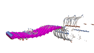
Figure 6 shows the flow structure visualised by isosurfaces of the Q-criterion (Hunt et al. Reference Hunt, Wray, Moin, Wray and Moin1988). For a direct comparison, the contour of the isosurface remains the same between the figures. The flow exhibits a distinguishable transition as  $\zeta$ increases. For low $\zeta$, the bumps dominate the flow structure, and we see distinct horseshoe vortices shed from each element. These vortices persist downstream into counter-rotating streaks that compose the near wake. The flow structures get smaller as $\zeta$ increases, and the horseshoe vortex around each element becomes less distinct. From figure 6(c) onwards, we can see that the near wake collects into a wavy vortex tube similar to those that categorise a two-dimensional flow driven by kinematics Zurman-Nasution et al. (Reference Zurman-Nasution, Ganapathisubramani and Weymouth2020).

Figure 6. The Q-criterion of the flow around a flat plate with a decreasing roughness wavelength. For longer wavelength roughness, the shedding off the bumps dominates the structures. As the wavelength decreases, the flow transitions to a predominantly two-dimensional state as the influence of the bump perturbations gives way to dominant kinematically driven structures.
Next, we study the influence of  $Re$ on the SPS flow by extending the range to $Re=6$, $12$ and $24\times 10^3$ (figure 7). The large-scale flow structures such as the leading-edge vortex and wake vortices remain similar, but increasing $Re$ is seen to greatly increase the production of small-scale vortices – both on the surface and in the wake. This is because the large-scale structures are driven by the kinematics and the surface topology, and the reduced viscosity causes the structures to break down quickly.

Figure 7. Flow structures of plates at  $Re=6$, $12$ and $24\times 10^3$ visualised by the same Q-criterion. The surface topographies, defined by $\lambda =1/8, 1/12, 1/16$, correspond to the enstrophy peaks discussed in § 3.4. The time evolution of these three flow fields are available as supplementary movies, available at https://doi.org/10. 1017/jfm.2023.703.
3.3. Forces
We find that increasing  $\zeta$ increases the power to maintain SPS (figure 8a) despite the strong two-dimensionality of the flow structures, which are normally associated with efficient power transfer (Zurman-Nasution et al. Reference Zurman-Nasution, Ganapathisubramani and Weymouth2020) as no energy is lost to three-dimensional effects. This means low $\zeta$ corresponding to the longer wavelength roughness, and associated three-dimensional flow structures are more efficient.

Figure 8. The key swimming performance and force characteristics of the plate at  $Re=12\,000$. (a) The power required to maintain SPS. (b) The side force RMS. (c) The time-averaged thrust. (d) The RMS thrust. The points making up the solid line are the rough simulations, and the dash-dotted line is a kinematically equivalent smooth simulation that matches $\zeta$ to the rough case.
Figure 8(b) shows that as  $\zeta$ increases, so does $RMS(C_L)$. This signals ineffective swimming as the side forces are balanced by the mass $\times$ acceleration of the body's motion, so larger side forces on an equally massive body cause the body to accelerate more side to side, decreasing the smoothness. Similarly, increasing $\zeta$ also increases $RMS(C_T)$ (figure 8d), leading to more of a surging motion, further decreasing the smoothness of the swimming. These signs of ineffective swimming are reflected in the stated increase in $\overline {C_P}$.
To decouple the roughness and wave speed effects, we run a smooth simulation with the same kinematics properties as in each rough case. This smooth kinematic counterpart gives a base flow to compare against the rough simulations, and the cycled average power and forces are shown in figure 8. Figure 8(c) illustrates that increasing  $\zeta$ for the smooth case increases $\overline {C_T}$, making the smooth-plate counterparts slightly thrust producing. The power $\overline {C_P}$ is reduced by adding roughness to the surface of the plate (figure 8a), for the shorter wavelength roughness tested. Shorter wavelength roughness also reduces $RMS(C_L)$ (figure 8b) and $RMS(C_T)$ (figure 8d), making the swimming more effective compared to a smooth, kinematic counterpart.
3.4. Enstrophy
So far, we have shown that surface roughness increases the drag on a surface, leading to inefficient swimming, and have identified variations in the flow structures for different textures and kinematics. To identify the separate fluid dynamic contributions of  $\zeta$ and $\lambda$, we look at scaled enstrophy of the rough surface and its smooth kinematic counterpart. We define the scaled enstrophy as
 \begin{equation} E = \frac{\displaystyle\int 0.5\,|\boldsymbol{\omega}|^2 \,{\rm d}V }{SA_1}, \end{equation}
where the scaling factor is the planform area times the motion amplitude to define an appropriate reduced volume over which to evaluate the mixing. We use the subscripts  $r, s$ to identify the rough and smooth cases, respectively.
In general, the enstrophy increases with  $Re$ because of the presence of smaller-scale structures (figure 7). We show this in figures 9(a,b), which report the results of $E$ against $\zeta$ for three $Re$ values. Figure 9(a) shows the results of the rough plate undergoing SPS, and figure 9(b) shows the enstrophy for the smooth, kinematic counterparts. Both the smooth and rough plates have an approximately linear increase that scales with $\log {Re }$.

Figure 9. (a) The  $\zeta$-dependent enstrophy for the rough SPS plates ( $E_r$) where higher $\zeta$ corresponds to lower $\lambda$. The circle, diamond and triangle markers correspond to $Re = 6$, $12$ and $24 \times 10^3$, respectively. (b) The enstrophy for the kinematically identical smooth plate $E_s$, where the dash-dotted line identifies the data as smooth, and the markers relating to $Re$ correspond as before. (c) The difference between the smooth and rough enstrophies, $\Delta E$, with respect to $\lambda /2\delta (Re)$. We take $\delta (Re)$ as the approximation of a laminar boundary layer thickness on a smooth, flat plate. The same markers are used to distinguish $Re$, and the colours orange, blue and green correspond to $Re = 6$, $12$ and $24 \times 10^3$ to aid in the distinction.
The positive gradient of both the smooth and rough enstrophies shows that enstrophy increases with  $\zeta$, and the offset between the smooth and rough lines indicates that adding roughness also increases enstrophy. As we increase $\zeta$, the enstrophy increases for both the smooth and rough cases. At the upper limit of $\zeta$, the smooth and rough lines start converging as the rough flow, like the smooth, becomes two-dimensional (figure 6).
One prominent feature of figure 9(a) is the peaks in enstrophy found for  $\zeta =1.1\unicode{x2013}1.3$. The peak in enstrophy coincides with the superposition of the flow features associated with both the roughness and kinematics (figure 7). This is evident as surfaces with shorter $\lambda$ are increasingly dominated by the two-dimensional vortex tubes associated with the kinematic flow as the structures shed of the roughness elements decrease in size (figures 6b–f), and surfaces with longer $\lambda$ are dominated by the flow off the roughness elements (figures 6a,b).
The mechanisms driving the peak in enstrophy are analogous to an amplification of flow structures found in Prandtl's secondary motions of the second kind (Nikuradse Reference Nikuradse1926; Prandtl Reference Prandtl1926), where secondary currents are induced when the surface texture has features that scale with the outer length scale of the flow. In fact, Hinze (Reference Hinze1967, Reference Hinze1973) found that secondary currents form when surface roughness has dominant scales comparable to the boundary layer thickness (or pipe/channel height). These secondary currents manifest as low- and high-momentum pathways in the flow (Barros & Christensen Reference Barros and Christensen2014) that are further sustained by spatial gradients (Anderson et al. Reference Anderson, Barros, Christensen and Awasthi2015). Vanderwel & Ganapathisubramani (Reference Vanderwel and Ganapathisubramani2015) identified that the spatial gradients and the strength of these secondary currents are maximised when the spanwise spacing between successive roughness features is approximately equal to the boundary layer thickness. When the spacing is small, the flow behaves more like a homogeneous rough surface. When the spacing is much larger than the secondary motions, the currents are spatially confined (and small) to the location of the roughness. The analogy to the case presented in this paper is not a direct comparison to Prandtl's secondary motions of the second kind as the flow is merely unsteady, although the system studied herein meets certain criteria – specifically, large-scale streamwise vortical structures (figures 6 and 7) driven from torque associated with anisotropy of the velocity fluctuations (Perkins Reference Perkins1970; Bottaro, Soueid & Galletti Reference Bottaro, Soueid and Galletti2006).
The increasing  $Re$ shifts the peak enstrophy in figure 9(a) towards higher $\zeta$ (lower $\lambda$), resulting in flow fields shown in figure 7. The enstrophy peaks occur at $\lambda =1/8$, $1/12$ and $1/16$ for $Re = 6$, $12$ and $24 \times 10^3$, respectively. In fact, estimating the value of $\delta (Re )$ by assuming a laminar boundary layer correlation ( $\delta (Re ) \approx 4.91{Re }^{-0.5}$), and leveraging an approximate scaling $\lambda /2\delta \approx 1$, yields results where $\lambda ( Re ) = 1/7.9$, $1/11.5$ and $1/15.8$ for $Re =6$, $12$ and $24 \times 10^3$. These estimations are remarkably close to the true enstrophy peaking wavelengths, so future studies can use this estimation to assess the importance of their dominant roughness length scales. The laminar boundary layer value of $\delta$ is taken since it is difficult to estimate a value of $\delta$ for the swimming plate. At these Reynolds numbers, $\delta$ could also be estimated using a turbulent boundary layer correlation ( $\delta \propto Re ^{0.2}$) since there is very little difference between the laminar and turbulent values.
Further, we can delineate the relationship between  $\lambda$ and the boundary layer thickness by plotting the normalised difference in enstrophy between the smooth and rough plates ( $\Delta E=(E_r-E_s)$) against $\lambda /2\delta (Re )$ (figure 9c). Figure 9(c) shows a strong collapse of the $\Delta E/E_s$ curves when plotted against $\lambda /2\delta (Re )$ for $Re=6$ and $12 \times 10^3$. The scaled maximum of both curves is 1.16 at $\lambda /2\delta (Re )$ just less than 1. The collapse breaks down at the highest $Re=24 \times 10^3$ because the flow on the smooth plate experiences a jump in $E_s$ at this Reynolds number, affecting the enstrophy differences.
Finally, in our study, the power increases almost linearly until  $\zeta \approx 1.8$ (figure 8a), and our enstrophy peak lies within this regime. This means that the accentuation of these secondary flows is truly a boundary layer scaling, and not a result of increased vorticity production at the wall, which would result in an increased force on the body. Therefore, we can relate the system's increase in mixing to scaling arguments defined previously in turbulent wall flows.
4. Conclusion
In this paper, we examined the effect of an egg-carton-type rough surface on a self-propelled swimming body. We varied the wavelength of the surface to understand how different surface topologies change the flow and performance of the swimmer. We found that a decrease in the roughness wavelength requires a greater wave speed to maintain self-propelled swimming. The greater wave speed changed the vortex structures and consolidated the vorticity into two-dimensional packets with a distinct leading-edge vortex propagating down the body. The long-wavelength rough surfaces were dominated by the shedding of horseshoe vortices from individual roughness elements that persisted in the wake. The thrust of the plate increased with wave speed, which was needed to overcome the drag induced by the roughness. The increased wave speed also increased the required power and the amplitude of the non-propulsive lift force. These increases implied that the plate was less efficient, less effective, and less steady in its swimming. To decouple the effects of roughness and kinematics, we compared the forces and enstrophy to a smooth swimmer with identical kinematics. We saw that, compared to the smooth cases, the roughness reduced the power required, as well as the amplitude of the lift and drag forces. There was a peak in enstrophy that coincided with a superposition of two flow modes, one dominated by three-dimensional structures and the other by the two-dimensional vortex tubes. The peak in enstrophy persisted over all three Reynolds numbers, and collapsed when the roughness wavelength was proportional to the boundary layer thickness. This spike in enstrophy is not a result of increased vorticity production at the wall because we do not have a corresponding increase in body force. Further, this boundary layer relationship is analogous to scaling arguments defined for turbulent wall flows (Vanderwel & Ganapathisubramani Reference Vanderwel and Ganapathisubramani2015).
These results show that you cannot ignore kinematics when assessing the performance of a swimmer with surface texture. Oeffner & Lauder (Reference Oeffner and Lauder2012) and Wen et al. (Reference Wen, Weaver and Lauder2014) reported an increase in speed and efficiency for their experiments, but we have shown that a change in wave speed dominates the thrust production of the plate. Adding a coating to a surface could increase the stiffness and thus increase the wave speed, causing the plate to swim faster. Another factor to consider is the structural resonance, which significantly affects the performance of flexible plates undergoing swimming (Quinn, Lauder & Smits Reference Quinn, Lauder and Smits2014). Any study attributing performance changes to surface textures must show the independence of their test cases to the kinematics.
We have identified nonlinear interactions between the roughness and kinematics that amplify this mixing without a nonlinear force or power increase. Other studies (Lang et al. Reference Lang, Motta, Hidalgo and Westcott2008; Afroz et al. Reference Afroz, Lang, Habegger, Motta and Hueter2016; Santos et al. Reference Santos2021) have identified the bristling of shark skin and conjectured that the increased mixing helps to keep flow attached in the flank region. This work is significant in understanding the hydrodynamic effect of surface textures on the flow and forces around a swimmer; it is the first study to look at surface textures on undulating surfaces with realistic and well-defined kinematics. However, it is limited in that the roughness elements are a hundred times larger than actual denticles, and  $Re$ is representative only of a small, slow-swimming shark.
Supplementary movies
Supplementary movies is available at https://doi.org/10.1017/jfm.2023.703.
Acknowledgements
We would like to thank the IRIDIS high performance computing facility, and its associated support at the University of Southampton, the Office of Naval Research Global Award N62909-18-1-2091.
Declaration of interests
The authors report no conflict of interest.
Appendix A. Resolution convergence
We tested resolutions of increasing powers of two for two surfaces where  $\lambda =1/16,1/52$ (figure 10). For figure 10(a), we measured the error against the value at the highest resolution, which contained $2.4\times 10^{9}$ grid cells. The pressure-based thrust $\overline {C_{T}}$ oscillates around a zero mean, so we measure the error in $\overline {C_{T}^2}$. We converge to below $4\,\%$ error for both surfaces. Our working resolution is at the lowest limit $\Delta x=0.004$, and figure 10(b) shows that the time history of $C_T$ also converges within this.

Figure 10. Resolution convergence for the rough SPS plate. (a) Error convergence of  $\overline {C_T^2}$. (b) Phase-averaged cycle where $\lambda =1/16$.
Figure 11 shows the convergence of the integral quantity of the  $x$ vorticity magnitude for the two surfaces where $\lambda =1/16,1/52$. We choose the surface where $\lambda =1/16$ because it is near this value that significant increases in enstrophy were found. We also test the surface where $\lambda =1/52$ because this represents the lowest limit of our surface resolution; for the proposed working resolution $\Delta x=0.004$, $5$ grid cells resolve the surface wavelength in the $x$ and $z$ directions. Furthermore, we measure $\int |\omega _x| \,{\rm d}V$ because it is zero for the two-dimensional smooth cases and therefore allows us to quantify the grid resolution independence of the topographic contribution to the flow. Again, we converged to within a reasonable limit at our working resolution $\Delta x=0.004$.

Figure 11. The convergence of  $\int |\overline {\omega _x}| \,{\rm d}V$ with simulation fidelity.
Appendix B. Domain study
We show the domain invariance of the solution by comparing the cycle average time series of  $C_T$. We compare the working domain (domain 1), of size $(18,20)$ and resolution $(1536,1536)$, to a much larger domain (domain 2), size $(9,4)$ and resolution $(3072,3072)$ (figure 12a). Figure 12(b) shows the cycle average time series of $C_T$ for the three $Re$ used in this study. For all three ( $Re=6,12, 24\times 10^3$), $C_T$ is plotted for domain 1 (solid line), and domain 2 (dotted line). For both domains, $C_T$ collapses, so the solution is domain-invariant.

Figure 12. The domain invariance of  $C_T$. (a) The relative size of the two-dimensional domains. The dotted line marks the extent of domain 2, where $(x, y) \in ([-4, 14], [-10, 10])$, and the solid line marks domain 1, where $(x, y) \in ([-2, 7], [-2, 2])$. (b) The thrust coefficient for $\zeta =1.06$ and $St=0.3$; the solid line for domain 1 and the dotted line of domain 2 are plotted on top of each other.
Appendix C. Experimental validation
First, we show that the method implemented in this study, set out in § 2.2, converges to a grid-independent solution. We perform simulations at  $St=0.3$, $\zeta =1.06$ and $Re = 6$, $12$ and $24\times 10^3$, with increasing resolution. In figure 13, we plot $C_T$ (phase-averaged over four cycles) and show that the resolution affects the time series minimally, to the point where different resolutions are barely distinguishable from each other.

Figure 13. The numerical convergence for the kinematic trajectory defined by (2.3) for  $\zeta =1.06$ and $St=0.3$.
Next, we validate our model by showing consistency with an experimental study (Lucas et al. Reference Lucas, Thornycroft, Gemmell, Colin, Costello and Lauder2015). We make minor alterations to our model to match the kinematic trajectory,  $St$ and $Re$ of a swimming plate. In Lucas et al. (Reference Lucas, Thornycroft, Gemmell, Colin, Costello and Lauder2015), they test four different plate stiffnesses and assess the swimming performance. Of these four plates, one (plate ‘ $1\_3$’) had an increasing amplitude envelope and a relatively constant wave speed, which ensures that the changes we need to match their conditions are minimal. Although Lucas et al. (Reference Lucas, Thornycroft, Gemmell, Colin, Costello and Lauder2015) test a range of different $St$ and $Re$, for the plate that we are matching, they provide only the kinematic trajectory for $Re=77\,000$ and $St=0.31$. Because of the sensitivity of the kinematic mode shape of a flexible plate to different excitation conditions (Quinn et al. Reference Quinn, Lauder and Smits2014), we can consider only the data point where $Re=77\,000$ and $St=0.31$.
Figure 14 shows a comparison of the raw and matched kinematic trajectories. We match the trajectory by minimising  $\|y(x,t)-\langle y(x,t) \rangle \|^2_2$, where $\langle y(x,t) \rangle$ is the model for the kinematics. We consider the amplitude envelope $A(x)$ and the wave speed $\zeta$ separately, and arrive at the functional form
 \begin{equation} \langle y(x,t) \rangle = a_i x^i \sin{(2{\rm \pi} (x/\zeta - f t))}, \end{equation}
where  $i_{0,1,2}=[0.072, 0.1685, -0.0701]$, and $\zeta = 2.15$. Furthermore, we measured the error in $\langle y(x,t) \rangle$ using
 \begin{equation} \sigma(y(x,t)-\langle y(x,t) \rangle)/\sigma(y(x,t))=0.076, \end{equation}
where  $\sigma (x) = \sqrt {\overline {(x-\bar {x})^2}}$ is the operator to compute the standard deviation. The raw data in Lucas et al. (Reference Lucas, Thornycroft, Gemmell, Colin, Costello and Lauder2015) do not match perfectly the idealised model of a swimmer, with slight asymmetry (figure 14) introducing the reported error.

Figure 14. The difference between the kinematic trajectories reported in Lucas et al. (Reference Lucas, Thornycroft, Gemmell, Colin, Costello and Lauder2015) and the fitted functional form (C1).
We have kept the domain size, grid refinement and time step constant in our working model, and altered only the kinematic trajectory,  $St$ and $Re$. This allows us to assess the accuracy of the computational set-up compared to Lucas et al. (Reference Lucas, Thornycroft, Gemmell, Colin, Costello and Lauder2015). As we increase the resolution, $\overline {C_T}$ converges to within $1.7\,\%$ of the reported experimental value (see table 1). This gives us confidence that the computational set-up is accurate and that the kinematics is implemented correctly.
Table 1. The convergence of  $\overline {C_T}$ to experimental results of Lucas et al. (Reference Lucas, Thornycroft, Gemmell, Colin, Costello and Lauder2015).

Appendix D. Tabulated forces
Tables 2–4 show  $\zeta, \overline {C_T}, \overline {C_P}$ for the rough and kinematically equivalent smooth simulations. Figure 8 is the graphical representation, but for ease of comparison, we have also tabulated the data.
Table 2. Tabulated data of simulations at  $Re=6000$ with the input roughness defined by $\lambda$ and corresponding $\zeta$ that result in SPS. The table also reports the values for $\overline {C_T}$, $\overline {C_P}$ where the subscript $s$ refers to a smooth plate for comparison.

Table 3. Tabulated data of simulations at  $Re=12\,000$ with the input roughness defined by $\lambda$ and corresponding $\zeta$ that result in SPS. The table also reports the values for $\overline {C_T}, \overline {C_P}$, where the subscript $s$ refers to a smooth plate for comparison.

Table 4. Tabulated data of simulations at  $Re=24\,000$ with the input roughness defined by $\lambda$ and corresponding $\zeta$ that result in SPS. The table also reports the values for $\overline {C_T}, \overline {C_P}$, where the subscript $s$ refers to a smooth plate for comparison.


 Open access