2. Continuum theory

2.1. Fluctuating hydrodynamics and electrokinetics

We consider a mesoscale system of electrolyte solution at thermal equilibrium in a periodic domain $\boldsymbol {\varOmega }$ of fixed volume. The system contains $S$ types of ionic species with concentration $c_\alpha (\boldsymbol {r},t)$ and charge valency $z_\alpha$ for the $\alpha$th ionic species. Let $e$ be the elementary charge. Then a global constraint is imposed by the charge neutrality condition

(2.1)\begin{equation} \sum_{\alpha=1}^{S} \int_{\boldsymbol{\varOmega}} e z_\alpha\,c_\alpha(\boldsymbol{r},t)\,{{\rm d}}\boldsymbol{r} = 0. \end{equation}

The solvent molecules are represented implicitly through their electrostatic and thermodynamic properties, such as dielectric constant $\epsilon$, bulk viscosity $\zeta$, and shear viscosity $\eta$. From the continuum perspective, this system can be described by equations of classical fluctuating hydrodynamics with an additional electrostatic force:

(2.2a)$$\begin{gather} \frac{\partial \rho}{\partial t} + \boldsymbol{\nabla} \boldsymbol{\cdot} \boldsymbol{g} = 0, \end{gather}$$

(2.2b)$$\begin{gather}\frac{\partial \boldsymbol{g}}{\partial t} + \boldsymbol{\nabla} \boldsymbol{\cdot} (\boldsymbol{g}\boldsymbol{v}) ={-} \boldsymbol{\nabla} p + \eta\,\nabla^{2}\boldsymbol{v} + \left(\frac{\eta}{3} + \zeta\right) \boldsymbol{\nabla}(\boldsymbol{\nabla}\boldsymbol{\cdot} \boldsymbol{v}) + \rho_e \boldsymbol{E} + \boldsymbol{\nabla} \boldsymbol{\cdot} \delta \boldsymbol{\boldsymbol{\varPi}}, \end{gather}$$

for velocity $\boldsymbol {v}(\boldsymbol {r}, t)$, pressure $p(\boldsymbol {r},t)$, mass density $\rho (\boldsymbol {r},t)$, momentum density $\boldsymbol {g}(\boldsymbol {r},t) = \rho (\boldsymbol {r},t)\, \boldsymbol {v}(\boldsymbol {r},t)$, and electric field $\boldsymbol {E}(\boldsymbol {r},t)$. The local charge density is given by $\rho _e(\boldsymbol {r},t) = \sum _{\alpha =1}^{S} e z_\alpha \, c_\alpha (\boldsymbol {r},t)$. The random stress tensor $\delta \boldsymbol {\varPi }$ is a matrix of Gaussian-distributed random variables with zero means and variances given by the fluctuation–dissipation theorem (FDT) (Ortiz & Sengers Reference Ortiz and Sengers2006)

(2.3)\begin{equation} \langle \delta \varPi_{ij}(\boldsymbol{r},t)\,\delta \varPi_{kl}(\boldsymbol{r}',t')\rangle = 2 k_BT \boldsymbol{\mathsf{C}}_{ijkl}\, \delta(\boldsymbol{r}-\boldsymbol{r}')\,\delta(t-t'), \end{equation}

where $\boldsymbol{\mathsf{C}}_{ijkl}=\eta (\delta _{ik}\delta _{jl} + \delta _{il}\delta _{jk})+(\zeta -{2\eta }/{3}) \delta _{ij}\delta _{kl}$ is a rank-4 tensor. The fluctuating hydrodynamic equations are closed with the equation of state, e.g. $c_s^{2} = (\partial p/\partial \rho )_T$, with $c_s$ being the isothermal sound speed.

The Ginzburg–Landau free energy functional for an electrolyte solution is (Ginzburg & Landau Reference Ginzburg and Landau1950)

(2.4)\begin{equation} G = \int_{\boldsymbol{\varOmega}} {{\rm d}}\boldsymbol{r} \left\{k_BT \sum_{\alpha=1}^{S} c_\alpha \ln c_\alpha + \sum_{\alpha=1}^{S} e z_\alpha c_\alpha \phi - \frac{\epsilon}{2}\,(\boldsymbol{\nabla}\phi)^{2}\right\}, \end{equation}

where $k_BT$ is the thermal energy, and $\phi$ is the electrostatic potential. Variation of the free energy with respect to the electrostatic potential yields the Poisson equation

(2.5)\begin{equation} {-}\boldsymbol{\nabla}\boldsymbol{\cdot} (\epsilon(\boldsymbol{r})\,\boldsymbol{\nabla}\phi) = \sum_{\alpha=1}^{S} e z_\alpha\,c_\alpha(\boldsymbol{r},t), \end{equation}

by setting $\delta G/\delta \phi = 0$. Similarly, the electrochemical potential of the $\alpha$th ionic species can be derived by variation with respect to ionic concentration:

(2.6)\begin{equation} \mu_\alpha = \frac{\delta G}{\delta c_\alpha} = k_BT \ln c_\alpha + z_\alpha e\phi. \end{equation}

The transport and dissipation of ionic species are driven by the fluid velocity, electrochemical potential and thermal fluctuations, which can be described in terms of the ionic concentration flux $\boldsymbol {J}(\boldsymbol {r},t)$ by

(2.7)\begin{equation} \frac{\partial c_\alpha(\boldsymbol{r},t)}{\partial t} + \boldsymbol{v}(\boldsymbol{r},t) \boldsymbol{\cdot}\boldsymbol{\nabla} c_\alpha(\boldsymbol{r},t) ={-}\boldsymbol{\nabla}\boldsymbol{\cdot}(\boldsymbol{J}_{\alpha}(\boldsymbol{r},t) + \delta \boldsymbol{J}_{\alpha}(\boldsymbol{r},t) ), \end{equation}

where $\boldsymbol {J}_{\alpha }(\boldsymbol {r},t)$ is the dissipative flux, and $\delta \boldsymbol {J}_{\alpha }(\boldsymbol {r},t)$ is the random flux when the system is near thermodynamic equilibrium. The diffusion flux can be written as $\boldsymbol {J}_\alpha = - \sum _{\beta =1}^{S} M_{\alpha \beta }\,\boldsymbol {\nabla } \mu _\beta (\boldsymbol {r},t)$, in which $\boldsymbol {\nabla } \mu$ is the thermodynamic force for diffusion flux, and $M_{\alpha \beta }$ are the Onsager coefficients related to macroscopic ionic diffusion coefficients. In general, $M_{\alpha \beta } = M_{\beta \alpha } \neq 0$, as implied by reversal invariance (Onsager Reference Onsager1931a,Reference Onsagerb). The off-diagonal terms $M_{\alpha \neq \beta }$ describe mutual diffusion and are assumed to be relatively small compared to the diagonal self-diffusion terms. For example, according to experimental data (Chapman Reference Chapman1967), the self-diffusion coefficients of cation and anion in a $1\,{\rm M}$ NaCl solution are $1.16\times 10^{-9}$ and $1.99\times 10^{-9}\,{\rm m}^{2}\,{\rm s}^{-1}$, respectively, while the mutual diffusion coefficient is one order of magnitude smaller: $1.3\times 10^{-10}\,{\rm m}^{2}\,{\rm s}^{-1}$. Therefore, we assume that the mutual diffusion terms can be ignored in the present work for simplicity. In numerical experiments, this assumption is checked by computing the self-diffusion and mutual diffusion coefficients from MD data using the Green–Kubo relations (Zhou & Miller Reference Zhou and Miller1996; Wheeler & Newman Reference Wheeler and Newman2004), as presented in § 3.

By substituting the electrochemical potential expression into the diffusion flux, we obtain

(2.8)\begin{equation} \boldsymbol{J}_\alpha ={-} M_{\alpha}\,\boldsymbol{\nabla} \mu_\alpha (\boldsymbol{r},t) ={-} \frac{M_{\alpha} k_BT}{c_\alpha}\,\boldsymbol{\nabla} c_\alpha - M_{\alpha}z_\alpha e\,\boldsymbol{\nabla} \phi. \end{equation}

In practice, it is more convenient to use the macroscopic diffusion coefficients $D_\alpha = {M_{\alpha } k_BT}/{c_\alpha }$ instead of the phenomenological coefficients $M_{\alpha }$. Therefore, the ionic concentration transport equation can be rewritten as

(2.9)\begin{equation} \frac{\partial c_\alpha(\boldsymbol{r},t)}{\partial t} + \boldsymbol{v}(\boldsymbol{r},t) \boldsymbol{\cdot}\boldsymbol{\nabla} c_\alpha(\boldsymbol{r},t)= \boldsymbol{\nabla}\boldsymbol{\cdot} \left(D_\alpha\,\boldsymbol{\nabla} c_\alpha + \frac{D_\alpha e z_\alpha c_\alpha}{k_BT}\,\boldsymbol{\nabla} \phi +\delta \boldsymbol{J}_{\alpha}(\boldsymbol{r},t)\right). \end{equation}

For a system near thermodynamic equilibrium, the random fluxes can be modelled as Gaussian random vectors with zero means and variance given by the generalized FDT as

(2.10)\begin{align} \langle \delta \boldsymbol{J}_{\alpha} (\boldsymbol{r},t) \boldsymbol{\cdot} \delta\boldsymbol{J}_{\beta}(\boldsymbol{r}',t')\rangle &= 2k_BT M_{\alpha \beta}\,\delta (\boldsymbol{r} -\boldsymbol{r}')\,\delta(t-t') \nonumber\\ &= 2 D_{\alpha} c_{\alpha}\,\delta (\boldsymbol{r}-\boldsymbol{r}')\,\delta(t-t'). \end{align}

The coupled equations (2.2)–(2.10) form the fluctuating hydrodynamic and electrokinetic equations.

2.2. Linearized theory of electrolyte solution

The stochastic partial differential equations (sPDEs) given by (2.2)–(2.10) could be solved through numerical discretization, with the FDT satisfied at the discrete level following the GENERIC framework (Grmela & Öttinger Reference Grmela and Öttinger1997; Öttinger & Grmela Reference Öttinger and Grmela1997). In general, it is very challenging to obtain an analytical solution of such sPDEs. However, if the local hydrodynamic and electrokinetic fluctuations are sufficiently small, then linear response theory can be applied to derive linearized equations to describe the relaxation process of electrolyte solution towards equilibrium. In the present work, we focus on the linearized equations for electrolyte solutions and their closed-form solutions.

The equilibrium state of a bulk electrolyte solution is characterized by its mean field properties, i.e. constant mass density $\rho _0$, constant pressure $p_0$, constant bulk ionic concentration $c_{\alpha 0}$, zero momentum field $\boldsymbol {g}_0 = 0$, and zero electrostatic potential field $\phi _0 = 0$. The local fluctuating hydrodynamic field can be expressed as the perturbation around the mean field state:

(2.11a)$$\begin{gather} \rho(\boldsymbol{r},t) = \rho_0 + \delta \rho(\boldsymbol{r},t), \end{gather}$$

(2.11b)$$\begin{gather}p(\boldsymbol{r},t) = p_0 + \delta p(\boldsymbol{r},t), \end{gather}$$

(2.11c)$$\begin{gather}\boldsymbol{g}(\boldsymbol{r},t) = \delta \boldsymbol{g} (\boldsymbol{r},t), \end{gather}$$

where the local perturbation of pressure can be related to density fluctuations via the equation of state $\delta p = c_s^{2}\,\delta \rho$ under isothermal conditions. Also, the local fluctuating electrostatic field can be decomposed as

(2.12a)$$\begin{gather} c_\alpha(\boldsymbol{r},t) = c_{\alpha 0} + \delta c_\alpha(\boldsymbol{r},t), \end{gather}$$

(2.12b)$$\begin{gather}\phi(\boldsymbol{r},t) = \delta \phi(\boldsymbol{r},t), \end{gather}$$

(2.12c)$$\begin{gather}\rho_e(\boldsymbol{r},t) = \delta \rho_e (\boldsymbol{r},t), \end{gather}$$

in which $\delta \rho _e(\boldsymbol {r},t) = \sum _{\alpha =1}^{S} e z_\alpha \,\delta c_\alpha (\boldsymbol {r},t)$ when the global electroneutrality condition $\sum _{\alpha =1}^{S} e z_\alpha c_{\alpha 0} = 0$ is imposed. The fluctuating electrostatic potentials and charge densities are related via the Poisson equation.

For small fluctuations of electrostatic field, the linearized fluctuating hydrodynamic and electrokinetic equations can be written as

(2.13a)$$\begin{gather} \frac{\partial (\delta \rho)}{\partial t} ={-}\boldsymbol{\nabla}\boldsymbol{\cdot} \delta \boldsymbol{g}, \end{gather}$$

(2.13b)$$\begin{gather}\frac{\partial (\delta \boldsymbol{g})}{\partial t} ={-}{c_s^{2}}\,\boldsymbol{\nabla} \delta \rho + \eta\,\nabla^{2} (\delta \boldsymbol{v}) + \left(\frac{\eta}{3}+\zeta\right) \boldsymbol{\nabla} (\boldsymbol{\nabla}\boldsymbol{\cdot}\delta \boldsymbol{v} ), \end{gather}$$

(2.13c)$$\begin{gather}\frac{\partial (\delta c_\alpha)}{\partial t} = \left(D_{\alpha}\,\nabla^{2} (\delta c_{\alpha}) + D_{\alpha}\, \frac{e z_{\alpha} c_{\alpha 0}}{k_BT}\,\nabla^{2} \delta \phi \right), \end{gather}$$

(2.13d)$$\begin{gather}-\boldsymbol{\nabla}\boldsymbol{\cdot} (\epsilon\,\boldsymbol{\nabla} \delta \phi) = \sum_{\alpha=1}^{S} e z_\alpha\,\delta c_\alpha(\boldsymbol{r},t), \end{gather}$$

where only first-order perturbation terms are kept in these linearized equations. It is important to note that the advection term $\boldsymbol {\nabla }\boldsymbol {\cdot }(\delta \boldsymbol {g}\,\delta \boldsymbol {v})$ and the electrostatic force $\delta \rho _e\, \boldsymbol {\nabla } \delta \phi$ in the momentum equation, and the convection term $\delta \boldsymbol {v} \boldsymbol {\cdot }\boldsymbol {\nabla } \delta c_\alpha$ in the transport equation, are high-order perturbation terms and are thus assumed to be negligible in the equations above. Therefore, the linearized hydrodynamic and electrokinetic equations become explicitly decoupled for fluid systems in thermodynamic equilibrium.

The linearized fluctuating hydrodynamic equations given by (2.13) can be transformed into $k$-space by a spatial Fourier transform and then solved in the $k$-space. Appendix A describes the detailed derivation of mass–momentum correlations by solving (2.13). The normalized temporal correlation functions of the mass–momentum fluctuations in the $k$-space are given by

(2.14a)$$\begin{gather} \frac{\langle \hat{\rho}(\boldsymbol{k},t)\,\hat{\rho}(\boldsymbol{k},0)\rangle}{\langle \hat{\rho}(\boldsymbol{k},0)\,\hat{\rho}(\boldsymbol{k},0)\rangle} = \exp(-\varGamma_T k^{2} t) \cos(c_s k t), \end{gather}$$

(2.14b)$$\begin{gather}\frac{\langle \hat{\boldsymbol{g}}_\parallel(\boldsymbol{k},t)\,\hat{\boldsymbol{g}}_\parallel(\boldsymbol{k},0)\rangle}{\langle \hat{\boldsymbol{g}}_\parallel (\boldsymbol{k},0)\,\hat{\boldsymbol{g}}_\parallel(\boldsymbol{k},0)\rangle} = \exp(-\varGamma_T k^{2} t) \cos(c_s k t), \end{gather}$$

(2.14c)$$\begin{gather}\frac{\langle\hat{\boldsymbol{g}}_\perp(\boldsymbol{k},t)\,\hat{\boldsymbol{g}}_\perp(\boldsymbol{k},0)\rangle}{\langle \hat{\boldsymbol{g}}_\perp (\boldsymbol{k},0)\,\hat{\boldsymbol{g}}_\perp(\boldsymbol{k},0)\rangle} = \exp(-\nu k^{2} t), \end{gather}$$

(2.14d)$$\begin{gather}\frac{\langle \hat{\rho}(\boldsymbol{k},t)\,{\rm i}\, \hat{\boldsymbol{g}}_\parallel(\boldsymbol{k},0)\rangle}{\langle \hat{\rho} (\boldsymbol{k},0)\,{\rm i}\, \hat{\boldsymbol{g}}_\parallel(\boldsymbol{k},0)\rangle} = \exp(-\varGamma_T k^{2} t) \sin(c_s k t), \end{gather}$$

where the symbol $\hat {~}$ indicates Fourier components, the wave vector $\boldsymbol {k} = (k, 0, 0)$ is defined along the (arbitrary) $x$-direction, $\nu = \eta /\rho$ is the kinematic viscosity, $\varGamma _T=2\nu /3+\zeta /2\rho$ is the sound absorption coefficient, and $c_s$ is the isothermal sound speed. Also, $\boldsymbol {g}_\parallel$ represents longitudinal momentum (sound mode) parallel to the wave vector $\boldsymbol {k}$, and $\boldsymbol {g}_\perp$ represents the transverse component (shear mode) perpendicular to the wave vector $\boldsymbol {k}$.

For simplicity in deriving closed-form solutions, we consider only two types of ionic species: the cation (denoted by $p$) and anion (denoted by $n$). By substitution of the Poisson equation into the linearized ionic transport equation, we obtain

(2.15a)$$\begin{gather} \frac{\partial(\delta c_p)}{\partial t} = D_p \left(\nabla^{2} (\delta c_p) + \kappa_p^{2}\,\delta c_p - \left| \frac{z_n}{z_p} \right| \kappa_p^{2}\,\delta c_n \right), \end{gather}$$

(2.15b)$$\begin{gather}\frac{\partial(\delta c_n)}{\partial t} = D_n \left(\nabla^{2} (\delta c_n) + \kappa_n^{2}\,\delta c_n - \left| \frac{z_p}{z_n} \right| \kappa_n^{2}\,\delta c_p \right), \end{gather}$$

where $\kappa _p^{2}$ and $\kappa _n^{2}$ are defined as

(2.16)\begin{equation} \kappa_p^{2} \equiv \frac{D_p {z_p}^{2} c_{p 0}e^{2}}{k_BT \epsilon},\quad \kappa_n^{2} \equiv \frac{D_n {z_n}^{2} c_{n 0}e^{2}}{k_BT \epsilon}, \end{equation}

with units of inverse-squared distance. For a periodic system, we can expand the solution in Fourier modes: $\delta c(\boldsymbol {r},t) = \sum _{\boldsymbol {k}}\delta \hat {c}(\boldsymbol {k},t) \,{\rm e}^{{\rm i}\boldsymbol {k}\boldsymbol {\cdot } \boldsymbol {r}}$. The spatial Fourier transformation of (2.15) gives two coupled ordinary differential equations

(2.17)\begin{equation} \left.\begin{gathered} \frac{\partial \delta \hat{c}_p(\boldsymbol{k},t)}{\partial t} = D_p \left[(\kappa_p^{2}-k^{2})\,\delta \hat{c}_p(\boldsymbol{k},t) - \left| \frac{z_n}{z_p} \right| \kappa_p^{2}\,\delta \hat{c}_n(\boldsymbol{k},t)\right], \\ \frac{\partial \delta \hat{c}_n(\boldsymbol{k},t)}{\partial t} = D_n\left[(\kappa_n^{2}-k^{2})\,\delta \hat{c}_n(\boldsymbol{k},t) - \left|\frac{z_p}{z_n} \right| \kappa_n^{2}\,\delta \hat{c}_p(\boldsymbol{k},t)\right]. \end{gathered}\right\} \end{equation}

The above equations can be written in matrix form as ${\partial \boldsymbol {u}(\boldsymbol {k},t)}/{\partial t} + \boldsymbol{\mathsf{L}}\boldsymbol {u} = 0$, with the vector $\boldsymbol {u} = (\delta \hat {c}_p, \delta \hat {c}_n)^\textrm {T}$, and $\boldsymbol{\mathsf{L}}$ the $2\times 2$ matrix defined as

(2.18) \begin{equation} \boldsymbol{\mathsf{L}} = \left[\begin{array}{@{}cc@{}} (k^{2} - \kappa_p^{2})D_p & \left|\dfrac{z_n}{z_p}\right|\kappa_p^{2} D_p \\ \left|\dfrac{z_p}{z_n}\right|\kappa_n^{2} D_n & (k^{2} - \kappa_n^{2}) D_n \\ \end{array}\right]. \end{equation}

The matrix $\boldsymbol{\mathsf{L}}$ can be further split as $\boldsymbol{\mathsf{L}} = -\boldsymbol{\mathsf{L}}_0 + k^{2} \boldsymbol{\mathsf{L}}_1$, where

(2.19)$$\begin{gather} \boldsymbol{\mathsf{L}}_0 = \left[ \begin{array}{@{}cc@{}} \kappa_p^{2} D_p & -\left|\dfrac{z_n}{z_p}\right|\kappa_p^{2} D_p \\ -\left|\dfrac{z_p}{z_n}\right|\kappa_n^{2} D_n & \kappa_n^{2} D_n \end{array}\right], \end{gather}$$

(2.20)$$\begin{gather}\boldsymbol{\mathsf{L}}_1 = \left[\begin{array}{@{}cc@{}} D_p & 0 \\ 0 & D_n \end{array}\right]. \end{gather}$$

These equations can be solved by a linear combination of the eigenvectors $\xi ^{(i)}(\boldsymbol {k})$, which satisfy the eigenvalue equation

(2.21)\begin{equation} [-\boldsymbol{\mathsf{L}}_0 + k^{2} \boldsymbol{\mathsf{L}}_1]\,\xi^{(i)}(\boldsymbol{k}) = \lambda_i\,\xi^{(i)}(\boldsymbol{k}). \end{equation}

The conditions $\kappa _{p, n}^{2} \gg k^{2}$ hold in the continuum limit, when either the domain size $L$ or the charge concentration $z_\alpha ^{2} c_{\alpha 0}$ is sufficiently large. In this limit, the eigenvalue equation can be solved perturbatively by expanding $\xi ^{(i)}$ and $\lambda ^{(i)}$ in powers of $k^{2}$:

(2.22a)$$\begin{gather} \xi^{(i)} = \xi_0^{(i)} + k^{2} \xi_1^{(i)} + \cdots , \end{gather}$$

(2.22b)$$\begin{gather}\lambda^{(i)} = \lambda_0^{(i)} + k^{2} \lambda_1^{(i)} + \cdots. \end{gather}$$

Substitution of (2.22) into the eigenvalue equation (2.21) gives the zero- and second-order perturbation theory equations:

(2.23a)$$\begin{gather} (\boldsymbol{\mathsf{L}}_0 - \lambda_0^{(i)}\boldsymbol{\mathsf{I}})\xi_0^{(i)} = 0, \end{gather}$$

(2.23b)$$\begin{gather}(\boldsymbol{\mathsf{L}}_0 - \lambda_0^{(i)}\boldsymbol{\mathsf{I}})\xi_1^{(i)} = (\boldsymbol{\mathsf{L}}_1 + \lambda_1^{(i)}\boldsymbol{\mathsf{I}}) \xi_0^{(i)}, \end{gather}$$

where $\boldsymbol{\mathsf{I}}$ denotes the identity matrix. The solution to order ${O}(k^{2})$ is given by two real negative roots approximated as $\lambda _1 \approx -((k^{2}+\kappa _p^{2})D_p + (k^{2}+\kappa _n^{2})D_n)+k^{2}\, D_s(k)$ (fast decay) and $\lambda _2 \approx -k^{2}\,D_s(k)$ (slow decay), where the collective diffusion coefficient of cation and anion pairs is defined as

(2.24)\begin{equation} D_s(k) = \frac{(k^{2} + \kappa_p^{2} + \kappa_n^{2})D_p D_n}{(k^{2}+\kappa_p^{2})D_p + (k^{2}+\kappa_n^{2})D_n}, \end{equation}

which has the same order as the diffusion coefficients $D_{\alpha }$. The solutions of (2.17) with initial conditions $\delta \hat {c}_p(\boldsymbol {k},0)$ and $\delta \hat {c}_n(\boldsymbol {k},0)$ can be written as

(2.25a)$$\begin{gather} \delta \hat{c}_p(\boldsymbol{k},t) = A_{1}\,\delta \hat{c}_p(\boldsymbol{k}, 0) + A_{2}\,\delta \hat{c}_n(\boldsymbol{k}, 0), \end{gather}$$

(2.25b)$$\begin{gather}\delta \hat{c}_n(\boldsymbol{k},t) = A_{3}\,\delta \hat{c}_n(\boldsymbol{k}, 0) + A_{4}\,\delta \hat{c}_p(\boldsymbol{k}, 0), \end{gather}$$

with the coefficients

(2.26a)$$\begin{gather} A_{1} = \alpha_p \,{\rm e}^{\lambda_1 t} + \alpha_n \,{\rm e}^{\lambda_2 t}, \end{gather}$$

(2.26b)$$\begin{gather}A_{2} = \beta_p({\rm e}^{\lambda_2 t} - {\rm e}^{\lambda_1 t}), \end{gather}$$

(2.26c)$$\begin{gather}A_{3} = \alpha_n \,{\rm e}^{\lambda_1 t} + \alpha_p \,{\rm e}^{\lambda_2 t}, \end{gather}$$

(2.26d)$$\begin{gather}A_{4} = \beta_n({\rm e}^{\lambda_2 t} - {\rm e}^{\lambda_1 t}), \end{gather}$$

where the dimensionless parameters are defined as

(2.27a)$$\begin{gather} \alpha_p = \frac{(k^{2} + \kappa_p^{2})D_p - k^{2}\,D_s(k)}{(k^{2} + \kappa_p^{2})D_p + (k^{2} +\kappa_n^{2})D_n - 2 k^{2}\,D_s(k)}, \end{gather}$$

(2.27b)$$\begin{gather}\alpha_n = \frac{(k^{2} + \kappa_n^{2})D_n - k^{2}\,D_s(k)}{(k^{2} + \kappa_p^{2})D_p + (k^{2} +\kappa_n^{2})D_n - 2 k^{2}\,D_s(k)}, \end{gather}$$

(2.27c)$$\begin{gather}\beta_p = \frac{\left|\dfrac{z_n}{z_p}\right|\kappa_p^{2} D_p}{(k^{2} + \kappa_p^{2})D_p + (k^{2} + \kappa_n^{2})D_n - 2 k^{2}\,D_s(k)}, \end{gather}$$

(2.27d)$$\begin{gather}\beta_n = \frac{\left|\dfrac{z_p}{z_n}\right|\kappa_n^{2} D_n}{(k^{2} + \kappa_p^{2})D_p + (k^{2} + \kappa_n^{2})D_n - 2 k^{2}\,D_s(k)}, \end{gather}$$

such that $\alpha _p + \alpha _n = 1$.

The fluctuations modelled by the above equations are transported and dissipated in time, and this can be shown via the time correlation of the fluctuating concentration field with different Fourier modes. The temporal correlations between species $\alpha$ and $\beta$ in the fluctuating concentration field are given by

(2.28)\begin{equation} \varPsi_{\alpha \beta} = \frac{\langle \delta \hat{c}_\alpha(\boldsymbol{k},t)\, \delta \hat{c}_\beta^{*}(\boldsymbol{k},0)\rangle}{\langle \delta \hat{c}_\alpha(\boldsymbol{k},0)\,\delta \hat{c}_\beta^{*}(\boldsymbol{k},0)\rangle}, \end{equation}

where the symbol $^{*}$ denotes the complex conjugate. The temporal correlation function for specific ionic species can then be expressed as

(2.29a)$$\begin{gather} \varPsi_{p p} = \alpha_p \,{\rm e}^{\lambda_1 t} + \alpha_n \,{\rm e}{}^{\lambda_2 t} + \beta_p S_{n p} ({\rm e}^{\lambda_2 t} - {\rm e}^{\lambda_1 t}), \end{gather}$$

(2.29b)$$\begin{gather}\varPsi_{n n} = \alpha_n \,{\rm e}^{\lambda_1 t} + \alpha_p \,{\rm e}{}^{\lambda_2 t} + \beta_n S_{p n} ({\rm e}^{\lambda_2 t} - {\rm e}^{\lambda_1 t}), \end{gather}$$

(2.29c)$$\begin{gather}\varPsi_{p n} = \alpha_p \,{\rm e}{}^{\lambda_1 t} + \alpha_n \,{\rm e}{}^{\lambda_2 t} + \frac{\beta_p}{S_{p n}}\, ({\rm e}^{\lambda_2 t} - {\rm e}^{\lambda_1 t}), \end{gather}$$

(2.29d)$$\begin{gather}\varPsi_{n p} = \alpha_n \,{\rm e}{}^{\lambda_1 t} + \alpha_p \,{\rm e}{}^{\lambda_2 t} + \frac{\beta_n}{S_{n p}}\,({\rm e}^{\lambda_2 t} - {\rm e}^{\lambda_1 t}), \end{gather}$$

in which $S_{p n}$ and $S_{n p}$ are static structure factor-like terms for a wave vector $\boldsymbol {k}$ defined as

(2.30a)$$\begin{gather} S_{p n}(\boldsymbol{k}) = \frac{\langle \delta \hat{c}_p(\boldsymbol{k},0)\, \delta \hat{c}_n^{*}(\boldsymbol{k},0)\rangle}{\langle\delta\hat{c}_n(\boldsymbol{k},0)\, \delta \hat{c}_n^{*}(\boldsymbol{k},0)\rangle}, \end{gather}$$

(2.30b)$$\begin{gather}S_{n p}(\boldsymbol{k}) = \frac{\langle \delta \hat{c}_n(\boldsymbol{k},0)\, \delta \hat{c}_p{*}(\boldsymbol{k},0)\rangle}{\langle\delta\hat{c}_p(\boldsymbol{k},0)\, \delta \hat{c}_p{*}(\boldsymbol{k},0)\rangle}. \end{gather}$$

In this linearized theory, the covariance between the initial ionic concentration fluctuations of cation and anion are non-zero due to the charge neutrality constraint. The structure factor terms $S_{p n}$ and $S_{n p}$ can be obtained from experiment or more detailed simulations. The long-time behaviour of both temporal autocorrelations and cross-correlations are dominated by slowly decaying terms that behave asymptotically as $\exp (\lambda _2 t)$, where $\lambda _2$ is one of the two (negative) eigenvalues.

3. Numerical results

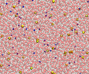
To validate the closed-form expressions of fluctuation correlations that we derived based on linearized fluctuating hydrodynamic and electrokinetic equations in § 2, we perform both all-atom MD simulations with explicit ions and mesoscale cDPD simulations with semi-implicit ions, as illustrated in figure 1. We first carry out all-atom MD simulations of an aqueous NaCl solution in the bulk, which consists of 400 Na$^{+}$ ions, 400 Cl$^{-}$ ions, and 64 000 H$_2$O water molecules in a periodic cubic computational domain with box size $L = 12.8\,\textrm {nm}$. The mass density is $\rho ^{0} = 0.616\,\textrm {amu}$ Å$^{-3}$, and the ion concentration is $c_{\pm } = 0.3168\,\textrm {M}$. The SPC/E model (Berendsen, Grigera & Straatsma Reference Berendsen, Grigera and Straatsma1987) is used for water molecules. The ionic force field terms are adopted from published work by Smith & Dang (Reference Smith and Dang1994) and Yoshida et al. (Reference Yoshida, Mizuno, Kinjo, Washizu and Barrat2014). The particle–particle particle-mesh (PPPM) method (Hockney & Eastwood Reference Hockney and Eastwood1988) is used for computing electrostatic interactions with vacuum periodic boundary conditions. The PPPM method maps atom charge to a three-dimensional mesh and uses fast Fourier transforms to solve Poisson's equation on the mesh, then interpolates electric fields on the mesh points back to the atoms, which is implemented in a built-in PPPM solver in LAMMPS (Thompson et al. Reference Thompson2022). A direct space cutoff of 9.8 Å, which is three times larger than the size of the oxygen atoms, is used to ensure the accuracy of the PPPM solver (Isele-Holder, Mitchell & Ismail Reference Isele-Holder, Mitchell and Ismail2012). The bond length of water molecules is constrained using the SHAKE algorithm (Ryckaert, Ciccotti & Berendsen Reference Ryckaert, Ciccotti and Berendsen1977) to allow a time step of $1\,\textrm {fs}$ in the velocity Verlet integrator (Allen & Tildesley Reference Allen and Tildesley2017). A constant number–volume–temperature system (NVT ensemble) is simulated at $T = 300\,\textrm {K}$ with a Nosé–Hoover thermostat. The system is relaxed for $0.5\,\textrm {ns}$ to achieve a thermal equilibrium state, and then for up to $10\,\textrm {ns}$ for statistics and sampling.

Figure 1. Typical snapshots of the aqueous NaCl solution from (a) all-atom MD simulations with explicit ions (box size $L=12.8\,\textrm {nm}$), and (b) mesoscale cDPD simulations with semi-implicit ions (box size $L=106.8\,\textrm {nm}$).

In § 2, we assumed that the mutual diffusion is small compared to ionic self-diffusion, thus it can be ignored in the derivation. To confirm this assumption, we compute both self-diffusion and mutual diffusion coefficients of ionic species from the MD velocity correlation functions via the Green–Kubo relationship (Zhou & Miller Reference Zhou and Miller1996; Wheeler & Newman Reference Wheeler and Newman2004). The computed self-diffusion coefficient is $1.3\times 10^{-9}\,\textrm {m}^{2}\,\textrm {s}^{-1}$ for Na$^{+}$, and $2.1 \times 10^{-9}\,\textrm {m}^{2}\,\textrm {s}^{-1}$ for Cl$^{-}$, while their mutual diffusion coefficient is $1.2 \times 10^{-10}\,\textrm {m}^{2}\,\textrm {s}^{-1}$. These results are consistent with previous simulation and experimental results for NaCl solutions (Wheeler & Newman Reference Wheeler and Newman2004), and also confirm that the mutual diffusion coefficient is much smaller than the self-diffusion coefficients in this electrolyte solution, thus it can be ignored in the analytical derivations of current correlation functions presented in § 2.

Alternative to all-atom MD simulation, at the mesoscopic scale, a cDPD model is used to tackle the challenge of simulating coupled fluctuating hydrodynamics and electrostatics with long-range Coulomb interactions. The cDPD model is an extension of the classical DPD model to solve numerically the fluctuating hydrodynamic and electrokinetic equations in the Lagrangian framework. In classical DPD models, ions can be represented by explicit charged particles with electrostatic interactions between explicit ions. Groot (Reference Groot2003) introduced a lattice to the DPD system to spread out the charges over the lattice nodes. Then the long-range portion of the interaction potential was calculated by solving the Poisson equation on the grid based on a PPPM algorithm (Hockney & Eastwood Reference Hockney and Eastwood1988) by transferring quantities (charges and forces) from the particles to the mesh, and vice versa. Because the mesh defines a coarse-grained length for electrostatic interactions, correlation effects on length scales shorter than the mesh size cannot be properly accounted for. Although the particle-to-mesh then mesh-to-particle mapping/redistribution can solve the Poisson equation for particle-based systems, its dependence on a grid may contradict the original motivation for using a Lagrangian method, and additional computational complexity and inefficiencies are introduced. To abandon grids and use a unifying Lagrangian description for mesoscopic electrokinetic phenomena, we developed the cDPD model (Deng et al. Reference Deng, Li, Borodin and Karniadakis2016) to solve the Poisson equation on moving cDPD particles rather than grids. More specifically, cDPD describes the solvent explicitly in a coarse-grained sense as cDPD particles, while the ion species are described semi-implicitly, i.e. using a Lagrangian description of ionic concentration fields, associated with each moving cDPD particle, as shown in figure 1(b), which provides a natural coupling between fluctuating electrostatics and hydrodynamics. The validation of the cDPD model has been confirmed by Deng et al. (Reference Deng, Li, Borodin and Karniadakis2016) in different problems, including electrostatic double-layer and electro-osmotic flows in micro-channels.

The state vector of a cDPD particle can be written as $(\boldsymbol {r}, \boldsymbol {v}, c_{\alpha }, \phi )$, which is characterized not only by its position $\boldsymbol {r}$ and velocity $\boldsymbol {v}$ as in the classical DPD model, but also by ionic species concentration $c_{\alpha }$ (with $\alpha$ representing the $\alpha$th ion type) and electrostatic potential $\phi$ on the particle. A cDPD system is simulated in a cubic periodic computational box with length $106.8\,\textrm {nm}$, where a cDPD particle is viewed as a coarse-grained fluid volume that contains the solvent and other charged species. Exchange of the concentration flux of charged species occurs between neighbouring cDPD particles, much like the momentum exchange in the classical DPD model. The governing equations of cDPD and model parameters are summarized in Appendix B. We will perform cDPD simulations of electrolyte solutions and compute current correlation functions of fluctuating electrokinetics to compare with theoretical predictions given in § 2.

We first examine the local fluctuations of mass density, momentum density, charge density and ionic concentration. For each of these quantities, we construct the instantaneous function $n(\boldsymbol {r})$ on a grid $\boldsymbol {r}^{i,j,k}$ by spatial averaging using a step function $W(r, h)$, with $h$ being the grid size, i.e. $W(r, h) = 1$ for $|\boldsymbol {r}_i-\boldsymbol {r}|\le 0.5h$, and $W(r, h) = 0$ for $|\boldsymbol {r}_i-\boldsymbol {r}| > 0.5h$. Then the local quantities can be extracted by $n(\boldsymbol {r}) = \sum _{i=1}^{N} W(|\boldsymbol {r} - \boldsymbol {r}_i|, h) n_i$ with $h = 3.1$ Å or $h = 7.75$ Å for MD data, and $h = 4.27\,\textrm {nm}$ for cDPD data. Because all instantaneous physical quantities are computed on a three-dimensional grid, the first point beyond $r = 0$ in spatial correlation functions (SCFs) presented in figures 3 and 4 is $r = h$, the second point is $r =\sqrt {2}h$, the third point is $r =\sqrt {3}h$, then $r =2h$, and so on. According to the central limit theorem, the local fluctuations in these quantities of interest should be Gaussian in the continuum regime. This is observed for mass density, momentum density and charge density from both MD and cDPD results. However, the local concentration fluctuations for ionic species in the MD system follow gamma distributions and converge to Gaussian with large spacing $h$, as shown in figure 2(a). Because the cDPD model assumes that the random fluxes of ionic concentration between neighbouring cDPD particles can be modelled by Gaussian white noises, the MD results indicate that the cDPD model is valid for length scales above a few nanometres, but has a lower bound for its length scale. Figure 2(b) presents the probability distribution functions of local ionic concentration in cDPD simulations, which follow a Gaussian distribution as expected.

Figure 2. Local ionic concentration probability distribution functions from (a) all-atom MD and (b) mesoscale cDPD simulations. The symbols show simulation data, while the lines show fits to gamma (MD) and Gaussian (inset of (a), and cDPD) distributions.

The SCFs for physical quantities of interest $n(\boldsymbol {r})$ are computed on the grid $\boldsymbol {r}^{i,j,k}$ according to

(3.1)\begin{equation} {\rm SCF}(\boldsymbol{r}) = \frac{1}{N(\boldsymbol{r})} \sum_{i=1}^{N(\boldsymbol{r})} \delta n(\boldsymbol{r}_i)\,\delta n(\boldsymbol{r}_i + \boldsymbol{r}), \end{equation}

where $N(\boldsymbol {r})$ is defined as a normalization coefficient. We have assumed that the spatial correlations are isotropic in weakly charged electrolyte bulk solutions. We observe that the spatial correlations of mass density, momentum density, charge density and ion concentration are all very short ranged (approximately delta-correlated for large systems), which is in agreement with continuum fluctuating hydrodynamics results at equilibrium. However, as shown in figure 3, there is small-scale anti-correlation structure for the charge densities obtained in the MD simulations. We also compute the SCF of charge density in mesoscale cDPD simulations, and find similar small-scale anti-correlation structures for both positive and negative ions, as shown in figure 4. These anti-correlation structures are observed on length scales comparable to the Bjerrum and Debye lengths for electrolyte solution systems, suggesting that this could be related to the ionic screening effect.

Figure 3. Spatial correlation function (SCF) of charge density from full-atom MD simulations for grid distances (a) $0.31\,\textrm {nm}$ and (b) $0.775\,\textrm {nm}$.

Figure 4. SCF of charge density from mesoscale cDPD simulations.

The temporal correlation function (TCF) between two physical quantities $u$ and $w$ in Fourier space is defined by

(3.2)\begin{equation} {\rm TCF}_k(t)=\langle u(\boldsymbol{k},t)\,w(\boldsymbol{k}, 0)\rangle = \frac{1}{N(t)} \sum_{s=1}^{N(t)} \hat{u}(\boldsymbol{k}, t)\,\hat{w}(\boldsymbol{k}, 0), \end{equation}

where $\boldsymbol {k}$ is the wave vector in Fourier mode, and $\hat {u}, \hat {w}$ are the Fourier components computed directly from particle trajectories as

(3.3)\begin{equation} \hat{u}(\boldsymbol{k},t) = \frac{1}{N_P} \sum_{i=1}^{N_P} u_i(\boldsymbol{r}_i, t) \exp(-{\rm i} \boldsymbol{k}\boldsymbol{\cdot}\boldsymbol{r}_i(t)). \end{equation}

We use a wavelength equal to the computational box size $L$ by setting $k=2{\rm \pi} /L$, which is $12.8\,\textrm {nm}$ for the MD system, and $106.79\,\textrm {nm}$ for the cDPD system.

Figures 5(a) and 5(b) present the temporal velocity autocorrelation functions from MD and cDPD simulations, respectively. The theoretical predication based on (2.14) gives $\textrm {CF}_v(t)=\exp (-0.1616t)$ (shear mode) and $\textrm {CF}_v(t)=\exp (-0.2403t)\cos (0.7352t)$ (sound mode) for the MD system, and $\textrm {CF}_v(t)=\exp (-0.0216t)$ (shear mode) and $\textrm {CF}_v(t)=\exp (-0.0238t)\cos (0.2177t)$ (sound mode) for the cDPD system. It can be observed from figure 5 that the computed results from both MD and DPD simulations are in agreement with the classical linearized theory of fluctuating hydrodynamics, i.e. the transverse autocorrelation function (shear mode) decays as $\exp (-\nu k^{2} t)$, with $\nu$ the kinematic shear viscosity, while the longitudinal autocorrelation function (sound mode) decays as $\exp (-\varGamma _T k^{2} t)\cos (c_s k t)$, with $\varGamma _T = 2\nu /3 + \zeta /2\rho$ the sound absorption coefficient and $c_s$ the isothermal sound speed. We conclude that the fluctuating hydrodynamics model still follows the classical linearized theory, and is not affected explicitly by the electrolyte bulk solutions. In an electrolyte solution in thermodynamic equilibrium, the fluctuating hydrodynamics and electrokinetics are decoupled explicitly.

Figure 5. Temporal transverse (shear mode) and longitudinal (sound mode) velocity autocorrelation functions in Fourier space from (a) MD and (b) cDPD simulations represented by open symbols, with comparison against the theoretical predictions in the form of (2.14) in solid and dashed lines.

Next, we compare the autocorrelation and cross-correlation functions of charge concentration with the linearized theory derived above, as shown in figure 6. We fit the MD and DPD results with the linearized theory in the form of (2.29) with proper structure factors $S_{p n}$ and $S_{n p }$, which are around $1.0$ and system-dependent, i.e.

(3.4)\begin{equation} \left.\begin{gathered} {\varPsi}_{pp}(t)={\varPsi}_{nn}(t)={-}0.0490\exp(\lambda_1 t) + 1.0049\exp(\lambda_2 t), \\ {\varPsi}_{pn}(t)={\varPsi}_{np}(t)=0.0276\exp(\lambda_1 t) + 0.9724\exp(\lambda_2 t), \end{gathered}\right\} \end{equation}

with $\lambda _1 = -7.4187\times 10^{-3}$ and $\lambda _2 = - 3.9067\times 10^{-4}$ for the MD system, and

(3.5)\begin{equation} \left.\begin{gathered} {\varPsi}_{pp}(t)={\varPsi}_{nn}(t)={-}0.2401\exp(\lambda_1 t) + 1.2401\exp(\lambda_2 t), \\ {\varPsi}_{pn}(t)={\varPsi}_{np}(t)=0.2458\exp(\lambda_1 t) + 0.7542\exp(\lambda_2 t), \end{gathered}\right\} \end{equation}

with $\lambda _1 = -3.4446\times 10^{-3}$ and $\lambda _2 = - 8.10\times 10^{-4}$ for the cDPD system. We observe in figure 6 that the computed results of temporal correlation functions from both MD and DPD simulations are in good agreement with the theoretical predictions derived from linearized theory of fluctuating hydrodynamics. Compared to the temporal correlation functions of hydrodynamic fluctuations presented in figure 5, the temporal correlations of charge concentration fluctuations shown in figure 6 decay extremely slowly over time. The long-time behaviour of both autocorrelation and cross-correlation follow the slow decay dominated by $\propto \exp (\lambda _2 t)$, which is significantly different from the decorrelation processes of hydrodynamic fluctuations.

Figure 6. Temporal cation and anion concentration autocorrelation ($\varPsi _{pp}$ and $\varPsi _{nn}$) and cross-correlation ($\varPsi _{pn}$ and $\varPsi _{np}$) functions in Fourier space from (a) MD and (b) cDPD simulations represented by open symbols, with comparison against the predictions from linearized fluctuating hydrodynamics theory in the form of (2.29) in solid and dashed lines.

4. Summary and discussion

We have presented theoretical closed-form expressions for the fluctuations of electrolyte bulk solution close to thermodynamic equilibrium, with an emphasis on mesoscopic spatiotemporal scales. In particular, we started with the Landau–Lifshitz theory and linearized the fluctuating hydrodynamic and electrokinetic equations to derive analytical solutions for current correlation functions using perturbation theory. To validate these theoretical expressions obtained based on the linearized theory, we performed numerical experiments of fluctuating hydrodynamics and electrokinetics for electrolyte solutions using both all-atom molecular dynamics (MD) and a mesoscale charged dissipative particle dynamics (cDPD) methods. We presented both MD and DPD simulation results of bulk electrolyte solutions in about 10 and 100 nm scales, which are compared directly with the predictions from the linearized continuum theory.

The current correlation functions computed from both MD and cDPD trajectories indicate that the temporal correlations of fluctuations from electrokinetics decay much more slowly than those from hydrodynamics, which agree well with the predictions made by the theoretical closed-form expressions of temporal correlation functions (hydrodynamics and charge) as well as the vast differences in decay time – varying by a few orders of magnitude. In a bulk electrolyte solution close to thermodynamic equilibrium, the fluctuating hydrodynamics and electrokinetics are decoupled explicitly because of the zero mean velocity, thus their behaviour is not dependent explicitly on the electrolyte concentrations in the dilute regime. At length scales above 10 nm, the results obtained from both MD and cDPD simulations are in good agreement with the continuum-limit linearized theories. The good agreement between the theoretical predictions and the particle-based mesoscopic simulations can also be interpreted as the capability of the mesoscopic cDPD model in bridging nano-to-continuum scales. Spatial correlations of charge density demonstrate finite range and non-trivial structure at nanometre length scales, but can be viewed as the delta function in the continuum limit. Simulation results also show that the fluctuations of local ionic concentration follow a gamma distribution at small length scales, while converging to a Gaussian distribution in the continuum limit, which suggests the existence of a lower bound of length scale for mesoscale models using Gaussian fluctuations for electrolyte solutions. Because the probability distribution functions of local ionic concentrations are computed directly from MD simulations before the continuum hypothesis is applied, a lower bound of length scale could exist in more general mesoscopic descriptions, including the Landau–Lifshitz PDE-based approach where stochastic fluxes are modelled as Gaussian processes.

It is worth noting that the present work focused on dilute electrolyte solutions close to thermodynamic equilibrium, where the mutual diffusion of ions is small compared to their self-diffusion, and the fluctuating electrokinetics is decoupled from zero-mean hydrodynamic fluxes. When the mutual diffusion coefficients of ions become comparable to the self-diffusion terms in concentrated electrolyte solutions (Dufrêche, Bernard & Turq Reference Dufrêche, Bernard and Turq2002; Galindres et al. Reference Galindres, Eslava, Ribeiro, Esteso, Vargas and Leaist2021), the contribution of mutual diffusion on ionic transport should be considered correctly in the fluctuating hydrodynamic and electrokinetic equations. Moreover, the linearized fluctuating hydrodynamics and electrokinetics system was solved in the $k$-space by a spatial Fourier transform, where the periodic condition is used in derivation of analytic solutions. Although both MD and cDPD simulations can be applied easily to electrokinetic problems involving fixed or induced charges on walls, the current theoretical framework cannot be extended to such problems directly. It is also interesting to consider how the fluctuating hydrodynamics is coupled with mesoscale electrokinetics in shear flows, where the current correction functions can be affected by the coupling between fluctuating terms and advection processes (Bian et al. Reference Bian, Deng and Karniadakis2018), leading to an orientation-dependent decorrelation process of fluctuating variables in the fluid system.