


1. Introduction
Man-made micro- and nanomotors have emerged as a potential agent for achieving many complicated tasks in in vivo and in vitro environments, such as active drug delivery (Luo et al. Reference Luo, Feng, Wang and Guan2018; Medina-Sánchez, Xu & Schmidt Reference Medina-Sánchez, Xu and Schmidt2018), assisted fertilization (Medina-Sánchez et al. Reference Medina-Sánchez, Schwarz, Meyer, Hebenstreit and Schmidt2016), environmental remediation (Gao & Wang Reference Gao and Wang2014), cargo transportation, biosensing (Park & Yossifon Reference Park and Yossifon2020) and many more. Micromotors built on the principle of self-phoretic propulsion (Moran & Posner Reference Moran and Posner2017), also known as Janus particles, gain motility by exploiting their engineered surface anisotropies that create local gradients of energies from the surrounding medium, thereby driving a fluid flow. These energy sources include chemical reaction (Paxton et al. Reference Paxton, Baker, Kline, Wang, Mallouk and Sen2006; Sánchez, Soler & Katuri Reference Sánchez, Soler and Katuri2015; Poddar, Bandopadhyay & Chakraborty Reference Poddar, Bandopadhyay and Chakraborty2019a), light (Xu et al. Reference Xu, Mou, Gong, Luo and Guan2017), electrical (Gangwal et al. Reference Gangwal, Cayre, Bazant and Velev2008; Lee et al. Reference Lee, Al Harraq, Bishop and Bharti2021) and magnetic fields (Chen et al. Reference Chen, Hoop, Mushtaq, Siringil, Hu, Nelson and Pané2017) etc. While the chemically powered motors are prone to fuel depletion in the environment and the bio-incompatibility posed by the use of toxic substances like  $\mathrm {H_2O_2}$ (Shields IV & Velev Reference Shields IV and Velev2017), the fuel-free actuation techniques, e.g. laser-induced thermal activation, can greatly circumvent such issues (Jiang, Yoshinaga & Sano Reference Jiang, Yoshinaga and Sano2010; Qian et al. Reference Qian, Montiel, Bregulla, Cichos and Yang2013).
An essential property of micromotors for their successful implementation in the applications mentioned above is their precise navigation towards targeted destinations in physiological pathways and environments. However, achieving deterministic motion over small length scales is restrained by the prominent Brownian diffusion associated with self-propulsion (Howse et al. Reference Howse, Jones, Ryan, Gough, Vafabakhsh and Golestanian2007). To deal with this intricacy, several external physical fields have been demonstrated to facilitate controlled directed motion of synthetic micro- and nanomotors (Tu, Peng & Wilson Reference Tu, Peng and Wilson2017). For catalytic propulsion, the fuel decomposition can be affected by changing the surrounding temperature, leading to improved speed control and efficiency (Balasubramanian et al. Reference Balasubramanian, Kagan, Manesh, Calvo-Marzal, Flechsig and Wang2009). Similarly, Baraban et al. (Reference Baraban, Makarov, Streubel, Monch, Grimm, Sanchez and Schmidt2012) showed that magnetic guidance of catalytic motors is possible by designing magnetic cap structures on the particles. Modulations in the speed and direction of the microswimming were achieved by tuning the strength and orientation of the applied field. Powered by tuneable motion characteristics, these micromotors can pick up cargo loads, transfer them to desired locations and even climb up vertical boundaries. In the work of Wang et al. (Reference Wang2018), the visible light source has been observed to enhance the motility of Ag/AgCl-based micromotors to a great extent.
Nature has enabled certain natural microorganisms to adjust their swimming appendages in response to a chemical signal in their environment (Yamamoto, Macnab & Imae Reference Yamamoto, Macnab and Imae1990; Krug, Riffell & Zimmer Reference Krug, Riffell and Zimmer2009), and the process is known as chemotaxis. Inspired by these natural processes, a significant volume of research was devoted to controlling self-phoresis using the gradient of one of the externally controlled fields like solute concentration (Baraban et al. Reference Baraban, Harazim, Sanchez and Schmidt2013; Popescu et al. Reference Popescu, Uspal, Bechinger and Fischer2018; Vinze, Choudhary & Pushpavanam Reference Vinze, Choudhary and Pushpavanam2021), light (Lozano et al. Reference Lozano, Ten Hagen, Löwen and Bechinger2016), electrostatic potential (Boymelgreen & Miloh Reference Boymelgreen and Miloh2012; Bayati & Najafi Reference Bayati and Najafi2019), temperature (Bickel, Zecua & Würger Reference Bickel, Zecua and Würger2014; Auschra et al. Reference Auschra, Bregulla, Kroy and Cichos2021) etc., and the mechanism is commonly termed taxis associated with the particular field type. The experiments of Baraban et al. (Reference Baraban, Harazim, Sanchez and Schmidt2013) revealed that self-diffusiophoretic micromotors could actively change their orientation and align their swimming direction with the applied chemical gradient. By doing this, they can search for the zones of high chemical concentration, which is a desirable swimming feature for targeted drug delivery where the micro- and nanomotors have to be steered towards a diseased site with an abnormal biochemical condition. Theoretical studies based on the pairwise chemotactic interaction (Saha, Golestanian & Ramaswamy Reference Saha, Golestanian and Ramaswamy2014) and Brownian dynamics simulation (Pohl & Stark Reference Pohl and Stark2014) for a collection of microswimmers reported the fascinating tendency of dynamic cluster formation among gradient-sensing microswimmers. In addition, the type of surface interaction between the active particles and the solvent fluid was predicted to play a major influencing role in the parallel or anti-parallel nature of the tactic motion (Bickel et al. Reference Bickel, Zecua and Würger2014; Saha et al. Reference Saha, Golestanian and Ramaswamy2014; Vinze et al. Reference Vinze, Choudhary and Pushpavanam2021). Among the studies on similar fuel-free phoretic mechanisms, the recent work of Auschra et al. (Reference Auschra, Bregulla, Kroy and Cichos2021) experimentally monitored the dynamic behaviour of a self-thermophoretic micromotor influenced by a localized thermal field originating from an optically heated gold nanoparticle. Their theoretical analysis based on a two-sphere interaction model in free space helped them describe the experimentally observed polarization effects and characterize the repelling and aligning interactions between self-phoresis and passive thermal effects. In addition to self-phoresis, the application of an external temperature gradient was found to be advantageous in the creeping motion of droplets (Panigrahi et al. Reference Panigrahi, Santra, Banuprasad, Das and Chakraborty2021; Mantripragada & Poddar Reference Mantripragada and Poddar2022).
In many of the microfluidic experiments dealing with microparticles actuated by external thermal sources (Weinert & Braun Reference Weinert and Braun2008; Di Leonardo, Ianni & Ruocco Reference Di Leonardo, Ianni and Ruocco2009; Lou et al. Reference Lou, Yu, Liu, Chen and Yang2018; Tsuji, Sasai & Kawano Reference Tsuji, Sasai and Kawano2018), the interaction with the confining substrates becomes inevitable, leading to modulations in the motion of the passive particles. A fascinating physical consequence of thermal gradient in the vicinity of a wall is the strong inter-particle attraction that facilitates stable two-dimensional crystals (Weinert & Braun Reference Weinert and Braun2008; Di Leonardo et al. Reference Di Leonardo, Ianni and Ruocco2009). Nevertheless, it remains an open question as to what consequence externally applied thermal gradients would have on a near-boundary auto-phoretic microswimmer. Very recently, various taxis mechanisms of micromotors have been focused on (Bayati & Najafi Reference Bayati and Najafi2019; Uspal Reference Uspal2019; Auschra et al. Reference Auschra, Bregulla, Kroy and Cichos2021; Vinze et al. Reference Vinze, Choudhary and Pushpavanam2021), but these studies were limited to the free-space dynamics of micromotors only, and the effects of a confining substrate were not considered. On the other hand, the near-wall dynamics of synthetic microswimmers is understood under the sole influence of self-phoresis (Uspal et al. Reference Uspal, Popescu, Dietrich and Tasinkevych2015b; Ibrahim & Liverpool Reference Ibrahim and Liverpool2016; Mozaffari et al. Reference Mozaffari, Sharifi-Mood, Koplik and Maldarelli2016; Poddar, Bandopadhyay & Chakraborty Reference Poddar, Bandopadhyay and Chakraborty2021).
To address the above shortcomings in the literature and noting the ever-increasing need for regulated motion of fuel-free micromotors, we formulate a theoretical model for a self-thermophoretic micromotor near a heat conducting plane wall, where the background fluid has a linearly varying temperature distribution due to external heating. The remote response of a micromotor to changes in the local thermal environment has been captured through the orientation of the gradient with respect to the wall-normal  $(\theta _T)$ and a dimensionless number $\mathcal {S}$, defined as the strength of the imposed thermal gradient relative to the thermal gradient that the coated hemisphere experiences due to laser irradiation. The bispherical coordinate system has been adopted to enforce the boundary conditions simultaneously at the particle surface and plane wall. We provide an exact solution of the thermal field under the assumption of negligible convection. Propulsive thrusts, both external and internal in origin, are evaluated using the reciprocal theorem for Stokes flows, thus avoiding the full solution of the flow field. Results indicate that a giant augmentation of the swimming speed can be achieved under the combined influence of external and self-phoretic actuation. Furthermore, here we provide concise phase-plane analyses for the near-wall dynamics, which turned out to constitute a convenient platform for easy sensitivity analysis of external parameters $\mathcal {S}$ and $\theta _T$. This starkly contrasts with the computationally intensive analysis of long-time solutions of the coupled differential equations adopted earlier. In addition, the non-hydrodynamic repulsive potential at the solid wall has been excluded here to concentrate on the hydrodynamic effects contributed by the externally regulated thermal source. The detailed demonstration of results highlights the combined actuation strategy as a promising means toward surpassing the limited scopes of on-demand control for autophoretic micromotors.
2. Problem formulation
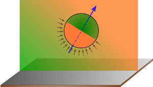
In the present problem, we consider a physical situation of a freely suspended thermally activated Janus particle (also known as a micromotor) near a conducting plane wall. The solvent fluid in which the particle is embedded is heated externally to establish a non-uniform temperature field  $\tilde {T}_\infty (\boldsymbol {x})$ (figure 1). The micromotor under consideration is usually fabricated from polystyrene or silica microbeads by coating half of the particle surface with a light-absorbing material (e.g. gold, titanium nitride) (Jiang et al. Reference Jiang, Yoshinaga and Sano2010; Ilic et al. Reference Ilic, Kaminer, Lahini, Buljan and Soljacic2016). The particle and fluid phase variables are denoted with the subscripts ‘ $p$’ and ‘ $f$’, respectively, e.g. $\varkappa _p$ and $\varkappa _f$ are the thermal conductivities of the two phases. When exposed to light irradiation by a laser beam with a heating power $Q$, a differential Joule heating of the two halves occurs due to the material asymmetry within the particle itself. The heat flux absorbed by the coated hemisphere can be calculated as $q''=Q/2{\rm \pi} R^2$ (Bregulla, Yang & Cichos Reference Bregulla, Yang and Cichos2014), where $R$ is the radius of the particle. Asymmetric heating of the two halves creates a local temperature gradient at the particle surface, which is treated as the self-induced or active temperature gradient in the present problem. This temperature variation along the surface originates a thermoosmotic slip velocity at the particle–fluid interface, which further causes an active thermophoretic thrust on the particle. The nature of the particle–fluid interaction (thermophilic/thermophobic) dictates the direction of thrust up or against the temperature gradient.

Figure 1. Schematic of a thermally activated half-coated Janus particle near a conducting plane wall. The surrounding fluid medium is externally heated using a linearly varying temperature field  $\tilde {T}_\infty$ along the direction $\boldsymbol {e}_T$. The green (cold) to orange (hot) coloured background denotes the variation of the external temperature field. Similarly, the orange and green colours on the particle denote the hot metallic cap and the cold uncoated halves of the particle surface, respectively. The symmetry axis of the Janus particle is oriented along $\boldsymbol {d}$. The plane conducting wall at $z=0$ has been marked with grey.
We impose a linearly varying temperature  $\tilde {T}_\infty (\boldsymbol {x})$ in the far field fluid medium, given as $\boldsymbol {\nabla } \tilde {T}_\infty = G_\infty \boldsymbol {e}_T$, where $\boldsymbol {e}_T$ is the unit vector defining the direction of the temperature gradient. The unit vector $\boldsymbol {e}_T$ can be related to the Cartesian unit vectors as $\boldsymbol {e}_T = \sin (\theta _T) \boldsymbol {e}_x + \cos (\theta _T) \boldsymbol {e}_z$, where $\theta _T$ is its orientation angle with the $z$ axis. A similar tilted temperature gradient may be created in a practical microfluidic setting by applying two separate temperature fields that linearly vary along the $x$ and $z$ directions, respectively. For example, Panigrahi et al. (Reference Panigrahi, Santra, Banuprasad, Das and Chakraborty2021) created a controlled linear temperature field along a direction parallel to the microchannel length ( $x$) using strip heaters. Again, a linear temperature field in the lateral direction $(z)$ can be obtained by preferentially heating the bottom or top wall of a microfluidic chamber by focusing laser beams (Di Leonardo et al. Reference Di Leonardo, Ianni and Ruocco2009). Finally, the above two linear temperature gradient components, while employed in tandem, may be tuned to maintain the desired tilt angle $(\theta _T)$ of the resultant temperature gradient vector $(\boldsymbol {\nabla } \tilde {T}_\infty )$.
The externally applied non-uniform temperature field also results in a thermophoretic slip at the particle surface, and a corresponding passive thermophoretic thrust is exerted on the particle. In situations of comparable flow strengths, this additional thrust-generating mechanism may interact with the active thrust and lead to non-intuitive locomotion attributes of the micromotor. This constitutes the central theme of the current analysis.
2.1. Governing equations and boundary conditions
With a focus on developing non-dimensional models for the temperature field and fluid flow and identifying the key dimensionless numbers, we normalize different variables with the following set of choices for the reference scales: length  ${\sim }R$; heat flux ${\sim }q''$; and thermal conductivity ${\sim }\varkappa _f$. Thus, the naturally evolving scales for temperature and velocity are ${\sim }q'' R/ \varkappa _f$, and ${\sim } - (\tilde {l}^2 \bar {\mathfrak {H}} q'' R/\mu T_0 \varkappa _f)$, respectively. Here, the parameters $\bar {\mathfrak {H}}$ and $T_0$ denote the characteristic magnitude of excess enthalpy and ambient temperature, respectively (Kroy, Chakraborty & Cichos Reference Kroy, Chakraborty and Cichos2016). In what follows, we drop the ‘ $\widetilde {}$ ’ symbol from different variables. In addition, $\mathcal {K} (=\varkappa _p/\varkappa _f)$ symbolizes the thermal conductivity ratio between the particle and fluid, and $\mathcal {T}$ stands for the dimensionless temperature. We also encounter a new dimensionless parameter $\mathcal {S} = G_\infty R/T_{ref} = G_\infty \varkappa _f/q''$, named the strength number, reflecting the relative strength of the characteristic heat fluxes due to the external temperature gradient and laser heating of the micromotor metal cap.
Low values of the Péclet number (see § 3 for details) allow the advective terms to be neglected in the energy equation, and the temperature distribution can be modelled in the quasi-static limit (Bickel, Majee & Würger Reference Bickel, Majee and Würger2013). Thus, employing the Fourier's law of heat conduction, the energy equation takes the form of the Laplace equation, both interior and exterior to the micromotor, given by
 \begin{equation} \nabla^{2}\mathcal{T}_{p,f} = 0. \end{equation}
Enforcing the finiteness of the temperature field inside the particle medium gives
 \begin{gather} \text{for}\
\sqrt{\rho^2+z^2} < 1,
\end{gather}
\begin{gather} \text{for}\
\sqrt{\rho^2+z^2} < 1,
\end{gather}
where  $\rho$ denotes the radial coordinate of cylindrical coordinate system ( $\rho, z, \phi$) and $\mathcal{T}_p$ is finite.
On the other hand, in the domain  $z > 0$, at large distances from the particle, the temperature gradient asymptotically attains the externally imposed condition $\boldsymbol {\nabla } \mathcal {T}_{f,\infty } = \mathcal {S} \boldsymbol {e}_T$. Further, the temperature field satisfies the following boundary condition at the conducting plane wall:
 \begin{equation} \text{at}\ z=0,\quad \mathcal{T}_f=\mathcal{T}_{ref} + \mathcal{S} \sin(\theta_T) x, \end{equation}
where  $\mathcal {T}_{ref}$ is a constant, which can be obtained from the temperature information of an arbitrary point in the domain.
The general solution of Laplace equation (Jeffery Reference Jeffery1912) as well as the creeping-flow velocity field (O'Neill Reference O'Neill1964) in a particle–wall configuration can be represented in terms of bispherical eigenfunctions. Furthermore, the velocity components are given in an associated cylindrical coordinate system  $(\rho, z, \phi )$. In view of using those general solutions, we define a bispherical coordinate system $(\xi,\eta,\phi )$ and relate it to the cylindrical coordinates by (Happel & Brenner Reference Happel and Brenner1983)
 \begin{equation} \tilde{\rho}=c\frac{\sin(\eta)}{\cosh(\xi)-\cos(\eta)} \quad \text{and} \quad \tilde{z}=c\frac{\sinh(\xi)}{\cosh(\xi)-\cos(\eta)}. \end{equation}
A corresponding diagrammatic depiction can be found in Poddar, Bandopadhyay & Chakraborty (Reference Poddar, Bandopadhyay and Chakraborty2020). In this bispherical system,  $\xi =0$ and $\xi =\xi _0$ denote the plane wall and the particle surface, respectively. In addition, the centre of the sphere is located at $\tilde {z}=\tilde {h}=c \coth (\xi _0)$. The positive scale factor $c$ can be related to the radius as $c = R \sinh (\xi _0)$. Similarly, we use the smallest distance between the particle surface and the wall $(\tilde {\delta })$, calculated as $\tilde {\delta }=\tilde {h}-R$, in our analysis.
In the next step, we leverage the linearity of the governing equation and the associated boundary conditions and calculate the temperature distribution as a superposition of the two sub-problems, as stated below
 $$\begin{gather} \mathcal{T}_f= \mathcal{T}_{f,sp} + \mathcal{T}_{f,ext} \end{gather}$$
 $$\begin{gather}\text{and} \quad \mathcal{T}_p= \mathcal{T}_{p,sp} + \mathcal{T}_{p,ext}. \end{gather}$$
Here,  $(\mathcal {T}_{f,sp} ,\mathcal {T}_{p,sp} )$ and $(\mathcal {T}_{f,ext} ,\mathcal {T}_{p,ext} )$ are obtained in sub-problem I and sub-problem II, respectively. Details of these sub-problems are given below.
(i) Sub-problem I: in this sub-problem, we consider the sole source of thermal energy as the laser heating of the micromotor metal cap. Within the realm of the ‘thin-cap limit’ (Jiang et al. Reference Jiang, Yoshinaga and Sano2010; Bickel et al. Reference Bickel, Majee and Würger2013; Poddar et al. Reference Poddar, Bandopadhyay and Chakraborty2021), the effect of heat release from the metallic coating is incorporated through a sudden change of heat flux $\mathcal {Q}(\boldsymbol {n}_{p})$ at the micromotor–solvent interface, given by
(2.7)where\begin{equation} \mathcal{Q}(\boldsymbol{n}_{p})=\begin{cases} 0, & \text{if}\ 0 \le \boldsymbol{d}\boldsymbol{\cdot} \boldsymbol{n}_p \le 1 \\ 1, & \text{otherwise}, \end{cases} \end{equation}$\boldsymbol {n}_p$ denotes the unit normal vector at the micromotor surface. Thus, the following form of the boundary condition holds at the micromotor surface:
(2.8)In this sub-problem, the temperature gradient vanishes at far distances from the particle, i.e.\begin{equation} \text{at}\ \xi=\xi_0,\quad -(\boldsymbol{\nabla} \mathcal{T}_{f,sp})\boldsymbol{\cdot}\boldsymbol{n}_p + \mathcal{K} (\boldsymbol{\nabla} \mathcal{T}_{p,sp})\boldsymbol{\cdot}\boldsymbol{n}_p = \mathcal{Q}(\boldsymbol{n}_p). \end{equation}(2.9)Also, due to the absence of an external temperature gradient, the fluid temperature at the plane wall remains constant and can be set to zero without loss of generality, i.e.\begin{equation} \text{at}\ (\rho^2+z^2)^{1/2}\to \infty,\quad \boldsymbol{\nabla} \mathcal{T}_{f,sp} \to 0. \end{equation}(2.10)From now on, we name this sub-problem as the self-propulsion problem (‘sp’).\begin{equation} \text{at} \quad \xi=0,\quad \mathcal{T}_f=0. \end{equation}
$\mathcal {Q}(\boldsymbol {n}_{p})$ at the micromotor–solvent interface, given by
(2.7)where\begin{equation} \mathcal{Q}(\boldsymbol{n}_{p})=\begin{cases} 0, & \text{if}\ 0 \le \boldsymbol{d}\boldsymbol{\cdot} \boldsymbol{n}_p \le 1 \\ 1, & \text{otherwise}, \end{cases} \end{equation}$\boldsymbol {n}_p$ denotes the unit normal vector at the micromotor surface. Thus, the following form of the boundary condition holds at the micromotor surface:
(2.8)In this sub-problem, the temperature gradient vanishes at far distances from the particle, i.e.\begin{equation} \text{at}\ \xi=\xi_0,\quad -(\boldsymbol{\nabla} \mathcal{T}_{f,sp})\boldsymbol{\cdot}\boldsymbol{n}_p + \mathcal{K} (\boldsymbol{\nabla} \mathcal{T}_{p,sp})\boldsymbol{\cdot}\boldsymbol{n}_p = \mathcal{Q}(\boldsymbol{n}_p). \end{equation}(2.9)Also, due to the absence of an external temperature gradient, the fluid temperature at the plane wall remains constant and can be set to zero without loss of generality, i.e.\begin{equation} \text{at}\ (\rho^2+z^2)^{1/2}\to \infty,\quad \boldsymbol{\nabla} \mathcal{T}_{f,sp} \to 0. \end{equation}(2.10)From now on, we name this sub-problem as the self-propulsion problem (‘sp’).\begin{equation} \text{at} \quad \xi=0,\quad \mathcal{T}_f=0. \end{equation}(ii) Sub-problem II: here, the effects of the external temperature gradient
$\boldsymbol {\nabla } \mathcal {T}_\infty (= \mathcal {S} \boldsymbol {e}_T)$ are considered alone, and the heat absorption at the particle surface due to laser irradiation is disregarded. Thus, the boundary condition at the particle surface for this problem is given by
(2.11)Contrary to the sub-problem I, far away from the particle, the temperature distribution reaches the externally applied temperature gradient, i.e.\begin{equation} \text{at}\ \xi=\xi_0,\quad (\boldsymbol{\nabla} \mathcal{T}_{f,ext})\boldsymbol{\cdot}\boldsymbol{n}_p = \mathcal{K}\ (\boldsymbol{\nabla} \mathcal{T}_{p,ext})\boldsymbol{\cdot}\boldsymbol{n}_p . \end{equation}(2.12)In addition, at the plane surface, the temperature distribution satisfies\begin{equation} \text{at}\ (\rho^2+z^2)^{1/2}\to \infty,\quad \boldsymbol{\nabla} \mathcal{T}_{f,ext} \to \mathcal{S} \boldsymbol{e}_T. \end{equation}(2.13)We name this problem as the external temperature gradient problem (‘ext’).\begin{equation} \text{at}\ \xi=0,\quad \mathcal{T}_{f,ext}=\mathcal{T}_{ref} + \mathcal{S} \sin(\theta_T) x. \end{equation}


In both the problems discussed above, the continuity of temperature at the particle–fluid interface is satisfied, i.e.  $\text {at}\ \xi =\xi _0, \mathcal {T}_f=\mathcal {T}_p$.
The temperature of the fluid phase in sub-problem II  $(\mathcal {T}_{f,ext})$ can be considered as a combination of the externally imposed temperature field $(\mathcal {T}_\infty )$ and the disturbance temperature field due to the presence of the micromotor $(\mathcal {T}_f^*)$
 \begin{equation} \mathcal{T}_{f,ext}=\mathcal{T}_\infty+\mathcal{T}_{f,ext}^*. \end{equation}
The imposed temperature field can be obtained by integrating the temperature gradient as
 \begin{equation} \mathcal{T}_\infty= \mathcal{T}_{ref} + \mathcal{S} \sin(\theta_T) x + \mathcal{S} \cos(\theta_T) z. \end{equation}
Using the above expression for  $\mathcal {T}_\infty$ and considering (2.14), (2.1) yields a Laplace equation for $\mathcal {T}^*_{f,ext}$
 \begin{equation} \nabla^2 \mathcal{T}^*_{f,ext}=0. \end{equation}
The solution of the above equation in terms of the bispherical eigenfunctions is given by (Jeffery Reference Jeffery1912)
 \begin{align} \mathcal{T}^*_{f,ext} &= \sqrt{\cosh \xi - \cos\eta} \sum_{m=0}^{\infty} \sum_{n=m}^{\infty} [A_{n,m}\sinh(n+1/2)\xi +B_{n,m}\cosh(n+1/2)\xi] \nonumber\\ &\quad \times P_n^{m}(\cos\eta)\cos(m\phi + \gamma_m), \end{align}
where  $P_n^{m}$ denotes the associated Legendre polynomial of degree ‘ $n$’ and order ‘ $m$’. On the other hand, the temperature distribution inside the micromotor must satisfy the finiteness condition at the centre of the micromotor. Hence, its general form can be expressed as (Subramanian & Balasubramaniam Reference Subramanian and Balasubramaniam2001)
 \begin{align} \mathcal{T}_{p,ext} = \sqrt{\cosh \xi - \cos\eta} \sum_{m=0}^{\infty} \sum_{n=m}^{\infty} d_{n,m} \exp({-(n+1/2)\xi}) P_n^{m}(\cos\eta)\cos(m\phi + \gamma_m). \end{align}
The unknown series coefficients in  $A_{n,m}, B_{n,m}$ and $d_{n,m}$ can be evaluated by using the following boundary conditions:
 $$\begin{gather} \text{at}\ \xi=0,\quad \mathcal{T}^*_{f,ext}=0, \end{gather}$$
 $$\begin{gather}\text{at}\ (\rho^2+z^2)^{1/2}\to \infty, \quad \boldsymbol{\nabla} \mathcal{T}^*_{f,ext} \to \boldsymbol{0}, \end{gather}$$
 $$\begin{gather}\text{at}\ \xi=\xi_0,\quad \mathcal{T}^*_{f,ext} = \mathcal{T}_{p,ext} \quad \text{and} \quad (\boldsymbol{\nabla} \mathcal{T}^*_{f,ext})\boldsymbol{\cdot}\boldsymbol{n}_p = \mathcal{K} (\boldsymbol{\nabla}\mathcal{T}_{p,ext})\boldsymbol{\cdot} \boldsymbol{n}_p. \end{gather}$$
The flow field around the micromotor follows the Stokes equation due to the low values of Reynolds number associated with such flows (Lauga & Powers Reference Lauga and Powers2009; Michelin & Lauga Reference Michelin and Lauga2014). Moreover, the incompressibility condition holds everywhere in the flow domain. Thus, the fluid flow satisfies (Happel & Brenner Reference Happel and Brenner1983; Poddar et al. Reference Poddar, Mandal, Bandopadhyay and Chakraborty2019c,Reference Poddar, Mandal, Bandopadhyay and Chakrabortyb)
 \begin{equation} \boldsymbol{\nabla}\boldsymbol{\cdot}{\boldsymbol{u}}=0 \quad \text{and} \quad -\boldsymbol{\nabla} {p}+ \nabla^2 {\boldsymbol{u}}=0. \end{equation}
The usual no-slip and no-penetration boundary conditions hold true at the plane wall, i.e. at  $\xi =0$, $\boldsymbol {u}\boldsymbol{\cdot}\boldsymbol {t}_w=0$ and $\boldsymbol {u}\boldsymbol{\cdot}\boldsymbol {n}_w=0$, respectively. With respect to the laboratory reference frame, the fluid velocity at the freely moving micromotor surface is given by the following boundary condition:
 \begin{equation} \text{at}\ \xi=\xi_0, \quad \boldsymbol{u} =\boldsymbol{V}+\boldsymbol{\varOmega} \times \boldsymbol{r}_{O'} + \boldsymbol{u}^s. \end{equation}
Here,  $\boldsymbol {u}^s$ is the tangential slip velocity of the solvent at the micromotor surface and is linked with the temperature distribution as (Anderson Reference Anderson1989; Kroy et al. Reference Kroy, Chakraborty and Cichos2016)
 \begin{equation} \boldsymbol{u}^s=\mathcal{M}_T (\boldsymbol{I-{n}{n}}) \boldsymbol{\cdot}\boldsymbol{\nabla} \left(\mathcal{T}_{sp}+\mathcal{T}_{ext}\right), \end{equation}
where  $\mathcal {M}_T =-\tilde {l}^2 \bar {\mathfrak {H}} / \mu T_0$ is defined as the thermophoretic mobility. The parameter $\mathcal {M}_T$ embodies the effects of the interaction of the solute molecules and the particle surface. Also, $\mathcal {M}_T > 0$ $( <0)$ indicates the interaction to be repulsive (attractive) in nature. In addition, in (2.23), $\boldsymbol {V}$ and $\boldsymbol {\varOmega }$ denote the translational and rotational velocities of the micromotor, respectively, and $\boldsymbol {r}_{O'}$ is the position vector relative to the micromotor centre.
The linearities of the Stokes flow and boundary condition in (2.24) indicate that the fluid velocity field can also be obtained as a superposition of the two sub-problems defined in the case of the temperature distribution, i.e.  $\boldsymbol {u} = \boldsymbol {u}_{sp}+\boldsymbol {u}_{ext}$.
It is noteworthy that the thermal conductivity of the particle material has a substantial impact on the temperature gradient at the particle surface, which directly influences the surface flow. This aspect of self-thermophoresis sets it apart from the widely studied self-diffusiophoresis problem, even in an unbounded domain (Poddar et al. Reference Poddar, Bandopadhyay and Chakraborty2021). A similar distinction exists between the passive thermophoresis sub-problem (‘ $\textit {ext}$’) and a comparable passive diffusiophoresis problem (Vinze et al. Reference Vinze, Choudhary and Pushpavanam2021). This is mathematically manifested through the boundary condition in (2.21a,b). Thus, the combined behaviour of the ‘ $\textit {sp}$’ and ‘ $\textit {ext}$’ sub-problems also depends on the thermal conductivity variation of the particle material.
2.2. Determining micromotor migration velocities
The unknowns  $\boldsymbol {V}$ and $\boldsymbol {\varOmega }$ can be determined when the additional constraints of force $(\boldsymbol {F})$- and torque $(\boldsymbol {C})$-free conditions for a neutrally buoyant micromotor are invoked as follows:
 \begin{equation} \boldsymbol{F}= \iint_{S_p} \boldsymbol{\sigma}\boldsymbol{\cdot}\boldsymbol{n_p}\,{\rm d} S=0 \quad \text{and}\quad \boldsymbol{C}= \iint_{S_p} \boldsymbol{r}_{O'} \times (\boldsymbol{\sigma}\boldsymbol{\cdot}\boldsymbol{n_p})\,{\rm d} S=0, \end{equation}
where  $S_p$ stands for the micromotor surface, and $\boldsymbol {\sigma }$ denotes the fluid stress tensor.
The force- and torque-free conditions applicable to the micromotor are a balance between the total forces/torques originating from two distinct phenomena, namely, the phoretic thrust generated due to the gradients in the temperature field  $(\boldsymbol {F}^{(Thrust)},\boldsymbol {C}^{(Thrust)})$, and the hydrodynamic resistance exerted due to rigid body motion $(\boldsymbol {F}^{(Drag)},\boldsymbol {C}^{(Drag)})$. The source of thrust is further divided into an active thermophoretic component $(\boldsymbol {F}^{(Thrust)}_{sp},\boldsymbol {C}^{(Thrust)}_{sp})$ and a passive thermophoretic component $(\boldsymbol {F}^{(Thrust)}_{ext},\boldsymbol {C}^{(Thrust)}_{ext})$. Hence, the force- and torque-free conditions read
 \begin{equation} \left.\begin{gathered} \boldsymbol{F}^{(Drag)}+\boldsymbol{F}^{(Thrust)}_{sp}+ \boldsymbol{F}^{(Thrust)}_{ext}=0 \\ \mathrm{and} \quad \boldsymbol{C}^{(Drag)}+\boldsymbol{C}^{(Thrust)}_{sp}+ \boldsymbol{C}^{(Thrust)}_{ext}=0, \quad \text{respectively.} \end{gathered}\right\} \end{equation}
The detailed steps for evaluating the drag forces/torques and active thermophoretic thrust can be found in Poddar et al. (Reference Poddar, Bandopadhyay and Chakraborty2021), and hence are not repeated here.
In order to evaluate  $\boldsymbol {F}^{(Thrust)}_{ext}$ and $\boldsymbol {C}^{(Thrust)}_{ext}$, we employ the Lorentz reciprocal theorem (LRT) (Happel & Brenner Reference Happel and Brenner1983) instead of solving the full flow field due to phoretic slip. In the present case, the LRT takes the form
 \begin{equation} \iint_{S_p} \boldsymbol{n}_p\boldsymbol{\cdot}\boldsymbol{\sigma}_{ext} \boldsymbol{\cdot}\boldsymbol{u}_{c}\,{\rm d} S=\iint_{S_p} \boldsymbol{n}_p \boldsymbol{\cdot}\boldsymbol{\sigma}_{c} \boldsymbol{\cdot} \boldsymbol{u}_{ext}\,{\rm d} S, \end{equation}
where ‘ $c$’ subscripted variables are associated with a complementary Stokes flow with similar geometry but a different boundary condition at the particle surface. The axisymmetry of the metallic cap about the director $\boldsymbol {d}$ and the in-plane orientation of the imposed temperature gradient $\boldsymbol {e}_T$ confine both the autonomous and the field-directed swimming in the $x-z$ plane. Therefore, the translational motion can be fully described by velocity components along $x$ and $z$ axes $(V_x,V_z)$.
The thrust torque and force exerted on a micromotor under thermotaxis in the vicinity of a wall are characteristically different from those for an isolated micromotor. Apart from the disturbances in the temperature field, the symmetry in the fluid stress distribution about the normal to the wall is also disrupted. Both these effects are known to combine, and as a result, the wall-parallel motion triggers a boundary-induced torque, which consequently gives rise to a non-zero rotational velocity of a self-propelled particle  $\boldsymbol {\varOmega }_{sp}$ along $\boldsymbol {e}_z \times \boldsymbol {V}_{sp}$ (Uspal et al. Reference Uspal, Popescu, Dietrich and Tasinkevych2015b; Mozaffari et al. Reference Mozaffari, Sharifi-Mood, Koplik and Maldarelli2016; Poddar et al. Reference Poddar, Bandopadhyay and Chakraborty2021). Along similar lines, the passive thermophoretic motion of a particle experiences a boundary-induced torque, which causes $\boldsymbol {\varOmega }_{ext}$ directed along $\boldsymbol {e}_z \times \boldsymbol {V}_{ext}$, i.e. the $y$ axis $(\varOmega _y)$. The thrust force components responsible for the three components of motion ${F}^{(Thrust)}_{ext,x}, {F}^{(Thrust)}_{ext,z}$ and ${C}^{(Thrust)}_{ext,y}$ can be calculated from (2.27) by using the complementary fluid stress tensors $(\boldsymbol { \sigma }_c)$ from the velocity field solutions provided in O'Neill (Reference O'Neill1964), Pasol et al. (Reference Pasol, Chaoui, Yahiaoui and Feuillebois2005) and Dean & O'Neill (Reference Dean and O'Neill1963), respectively. The different convergent infinite series for temperature and complementary velocity fields have been truncated at a large number of terms $n = N$, which gives a relative accuracy ${\approx }10^{-6}$ between the consecutive series coefficients as well as the key dynamic variables, i.e. $V_x, V_z,\varOmega _y$. Furthermore, the evaluation of $V_z$ requires the series expansion for $m = 0$ only on account of the azimuthal symmetry. On the other hand, a resolution until $m=1$ of different variables is required for evaluating $V_x$ and $\varOmega _y$.
3. Results and discussion
With an aim to demonstrate our results in a practically relevant parametric space, we look into the different practical scenarios encountered in the related experimental literature. We consider the imposed temperature gradient as  $O(1)\ \textrm {K}\,\mathrm {\mu }\textrm {m}^{-1}$ (Tsuji et al. Reference Tsuji, Sasai and Kawano2018), while the thermophoretic particles usually have diameters of $1$ to $10\,\mathrm {\mu }\textrm {m}$ (Weinert & Braun Reference Weinert and Braun2008; Di Leonardo et al. Reference Di Leonardo, Ianni and Ruocco2009). Also, taking the fluid medium as a water–glycerol mixture gives a thermal conductivity as $\varkappa _f =0.54$ W mK $^{-1}$ (Weinert & Braun Reference Weinert and Braun2008). In addition, considering the optical heating of Janus particles, the absorbed power $(Q)$ is in the range 3–150 mW (Bregulla et al. Reference Bregulla, Yang and Cichos2014). Using these practical dimensional values, the dimensionless strength number can be estimated as $\mathcal {S} \sim O(10^{-3}-10^{-1})$. A non-uniform temperature field in the solvent fluid can be produced by laser heating on a microchannel, similar to the experiments of Tsuji et al. (Reference Tsuji, Sasai and Kawano2018). Other possible microfluidic experimental set-ups may include a strip heater (Panigrahi et al. Reference Panigrahi, Santra, Banuprasad, Das and Chakraborty2021) or circulating hot and cold water flows (Mao, Yang & Cremer Reference Mao, Yang and Cremer2002). Since the temperature gradient in the latter set-ups can be regulated externally, it alleviates the complexities of simultaneous laser heating of the particles and the fluid. Furthermore, we consider the thermal conductivity ratio as $\mathcal {K} = 1$ (Jiang et al. Reference Jiang, Yoshinaga and Sano2010; Bickel et al. Reference Bickel, Majee and Würger2013) in the following demonstrations to limit the parametric space and focus only on the interaction between the autonomous and field-driven phoretic motion. Also, the results are provided for excess enthalpy $\bar {\mathfrak {H}}<0$, leading to positive phoretic mobility $(\mathcal {M}_T>0)$ for both the metallic (e.g. gold) and the polymeric (e.g. polystyrene) halves of the Janus particle, similar to the recent experimental observations of Auschra et al. (Reference Auschra, Bregulla, Kroy and Cichos2021). Moreover, the thermophoretic velocity $\tilde {u}_T$ in related experiments (Jiang et al. Reference Jiang, Yoshinaga and Sano2010; Qian et al. Reference Qian, Montiel, Bregulla, Cichos and Yang2013; Tsuji et al. Reference Tsuji, Sasai and Kawano2018) was reported to be of the order of $10\,\mathrm {\mu } \textrm {m}\ \textrm {s}^{-1}$, and a realistic thermal diffusion coefficient can be estimated as $D \sim 10^{-9}- 10^{-10}\ \textrm {m}^2\ \textrm {s}^{-1}$. Thus, the value of the Péclet number, defined as $Pe = \tilde {u}_T a/D$, remains well below unity, i.e. $Pe \ll 1$, justifying the assumption of negligible convection effects in § 2.1.
3.1. An isolated micromotor under thermotaxis
Before unveiling the wall-induced complexities, it is important to develop insights into the combined interplay between the active and passive thermophoresis phenomena in an unbounded domain. Following Uspal et al. (Reference Uspal, Popescu, Dietrich and Tasinkevych2015b), an unconfined self-phoretic particle shows rotational motion  $(\varOmega _{y,sp} \ne 0)$ only when its mobility coefficient is non-uniform over the two halves of its surface. In the present work, we consider a uniform mobility coefficient; hence, we encounter $\varOmega _{y,sp} = 0$. Similarly, it was also reported that rotation of an unbounded inert sphere under a linearly varying solute density exists only under varying surface mobility (Popescu et al. Reference Popescu, Uspal, Bechinger and Fischer2018; Vinze et al. Reference Vinze, Choudhary and Pushpavanam2021), indicating $\varOmega _{y,ext} = 0$. As a resultant effect, a particle under both active and passive sources of thermal gradients has been observed to exhibit zero rotational velocity in the unbounded domain, i.e. $\varOmega _y = \varOmega _{y,sp} + \varOmega _{y,ext} =0$.
It is evident that, for an unbounded micromotor, the temperature distribution has azimuthal symmetries about the axes  $\boldsymbol {d}$ and $\boldsymbol {e}_T$ for the ‘sp’ and ‘ext’ problems, respectively. Under the simultaneous action of the two physical mechanisms, the resultant temperature gradient in the unbounded domain can be written as
 \begin{equation} |\boldsymbol{\nabla} \mathcal{T}| \boldsymbol{e}_{res}= |\boldsymbol{\nabla} \mathcal{T}_{sp}| (-\boldsymbol{d})+ \mathcal{S} |\boldsymbol{\nabla} \mathcal{T}_{ext} | \boldsymbol{e}_T, \end{equation}
where the symmetry axis of the unbounded temperature profile directs along a resultant axis  $\boldsymbol {e}_{res} = \boldsymbol {\nabla } \mathcal {T} / |\boldsymbol {\nabla } \mathcal {T} |$. Consequently, the symmetry of the resultant temperature field depends on the strength number $\mathcal {S}$. It is to be noted that, in an unbounded scenario, the chosen negative value of the excess enthalpy $(\bar {\mathfrak {H}}<0)$ leads to a temperature gradient directed opposite to the orientation $\boldsymbol {d}$ (Bickel et al. Reference Bickel, Majee and Würger2013). This is manifested through the $- \boldsymbol {d}$ direction associated with $|\boldsymbol {\nabla } \mathcal {T}_{sp}|$ in the above equation.
For a particle under either passive or active thermophoresis, the direction of its surface velocity depends on the sign of the mobility coefficient  $\mathcal {M}_T$ and the direction of the temperature gradient, as indicated by (2.24). Now, for the chosen negative excess enthalpy $(\bar {\mathfrak {H}}<0)$, the phoretic mobility $(\mathcal {M}_T )$ (see after (2.24)) becomes positive. In the case of an unbounded auto-thermophoretic Janus particle, this implies a phoretic velocity directed towards the uncoated (colder) half of the particle, i.e. along the orientation vector, i.e. $+\boldsymbol {d}$ (Bickel et al. Reference Bickel, Majee and Würger2013; Poddar et al. Reference Poddar, Bandopadhyay and Chakraborty2021). On the other hand, for a positive external temperature gradient $\mathcal {S} \boldsymbol {e}_T$, a passive particle is bound to move towards the colder region of the background field. However, in case of an active particle in an externally maintained temperature field, the orientation of the hot and cold halves relative to the external gradient further complicates the scenario due to highly non-homogeneous heat release by the particle surface. Thus, the thermally active Janus colloids can show either positive or negative thermotaxis, defined as its motion towards the hotter or colder regions of the background field, respectively, even for a fixed sign of phoretic mobility $\mathcal {M}_T$. To identify the tendency of the micromotor to show positive or negative thermotaxis, we resolve its swimming speed parallel and perpendicular to the applied temperature gradient as
 $$\begin{gather} {\text{for}\ \mathcal{S} \ne 0},\quad \boldsymbol{V}= \boldsymbol{V}^{\parallel} +\boldsymbol{V}^{{\perp}}, \end{gather}$$
 $$\begin{gather}\text{where}\ \boldsymbol{V}^{\parallel} =V^{\parallel}\boldsymbol{e}_T =(V_{ext}+V_{sp} (\boldsymbol{d}\boldsymbol{\cdot} \boldsymbol{e}_T)) \boldsymbol{e}_T \quad \text{and} \quad \boldsymbol{V}^{{\perp}} = V_{sp} \, \boldsymbol{d}\boldsymbol{\cdot} (\boldsymbol{I}-\boldsymbol{e}_T \boldsymbol{e}_T). \end{gather}$$
Figure 2(a) depicts a regime map for positive and negative thermotaxes based on the values  $V^\parallel$ in the $\mathcal {S}$– $\theta _T$ plane. It has been found that for $\mathcal {S} > 0.25$, the negative thermotaxis is the only behaviour irrespective of the orientation of the external field with respect to the micromotor director $(\theta _T)$. On the other hand, below this critical strength number $\mathcal {S}$, the locomotion towards or away from the hotter zone is dictated by the competitive effects of varying orientation $\theta _T$ and the relative strength of the external temperature gradient $\mathcal {S}$. Also, the positive thermotaxis occurs only for $0^{\circ } \le \theta _T \le 90^{\circ }$ and $270^{\circ }\le \theta _T \le 360^{\circ }$. The $V^{\parallel } = 0$ lines in the same figure signify the combinations of the parameters $(\mathcal {S},\theta _T)$ for which the active and passive thermophoretic components balance each other along $\boldsymbol {e}_T$, and the micromotor swims perpendicular to external temperature gradient.

Figure 2. Velocity of the micromotor in the unbounded domain. (a) Regime diagram for positive and negative thermotaxes based on  $V_{\parallel }$ in the $\mathcal {S}$– $\theta _T$ plane. Variations of (b) translational velocity magnitude $(|\boldsymbol {V}|)$, and (c) orientation of the velocity vector $({\rm \Delta} \theta _v)$ with the orientation angle of the background temperature field $(\theta _T)$ for different values of the strength number $(\mathcal {S})$. In (b), the dashed lines are ‘ext’ cases, and the marker lines are combined situations for the indicated $\mathcal {S}$.
The variation of the swimming velocity magnitude  $|\boldsymbol {V}|$ in the unbounded domain with $\theta _T$ for various $\mathcal {S}$ has been portrayed in figure 2(b). The isolated particle velocities under passive thermophoresis (shown with dashed lines) for different $\mathcal {S}$ values match exactly with the reported results of Brock (Reference Brock1962): $\boldsymbol {V}_{ext}= - 2\mathcal {K}\mathcal {S}/(2\mathcal {K}+1) \boldsymbol {e}_T$. As depicted in the same figure, a Janus colloid under self-thermophoresis has a speed of $|\boldsymbol {V}_{sp}| = 0.167$. On the other hand, for some low external field strengths $\mathcal {S} \le 0.25$, passive thermophoresis gives rise to a lower swimming speed than self-propulsion $|\boldsymbol {V}_{ext}| < |\boldsymbol {V}_{sp}|$, while the converse happens beyond this critical $\mathcal {S}$. The combined interplay of the active and passive temperature gradients induces several interesting aspects of the micromotor velocity. For some intermediate external field orientations, the external gradient induces greater swimming speeds to the micromotor than its self-propelled counterpart, i.e. $|\boldsymbol {V}| > |\boldsymbol {V}_{sp}|$, while other orientations give a lesser swimming speed, i.e. $|\boldsymbol {V}| < |\boldsymbol {V}_{sp}|$. Furthermore, these ranges of $\theta _T$ responsible for distinct swimming action vary as the strength number $\mathcal {S}$ increases.
An unbounded self-thermophoretic micromotor swims along its symmetry axis  $\boldsymbol {d}$. However, a simultaneously acting external temperature gradient disrupts this symmetry or temperature distribution, and the micromotor swims along a direction that makes an angle ${\rm \Delta} \theta _v$ with $\boldsymbol {d}$. The variation of this swimming angle ${\rm \Delta} \theta _v$ with the external gradient orientation for different strength numbers $\mathcal {S}$ has been portrayed in figure 2(c). Variation of $\theta _T$ in the 3rd and 4th quadrants causes swimming angles to retain in the 1st and 2nd quadrants. The figure shows, the external gradient directed opposite to the internal symmetry, i.e. $\theta _T=180^{\circ }$, augments the self-propulsive action and causes swimming along $\boldsymbol {d}$ only. The augmentation of swimming speed in these scenarios is only $4\,\%$ with $\mathcal {S} = 0.01$, but rises up to $40\,\%$ and $100\,\%$ with $\mathcal {S}= 0.1$ and 0.25, respectively. Another limit is set by the case of passive thermophoresis, in which case the swimming occurs along $\boldsymbol {e}_T$ only. It is found that the deviation of the swimming axis from the director is maximum at some intermediate values of $\theta _T$ when the strength number is $\mathcal {S} \le 0.25$. Beyond this strength number $\mathcal {S}$, a monotonic increase of ${\rm \Delta} \theta _v$ takes place.
3.2. Thermotaxis near a plane wall
How do the boundary effects induced by a nearby planar wall affect the locomotion characteristics of a micromotor under thermotaxis? To answer this question, we sequentially discuss the corresponding effects on the temperature distribution and micromotor migration velocity. Subsequently, we analyse the trajectories of the micromotor under different wall distances, orientations relative to the wall and parameters of the external temperature field.
3.2.1. Temperature distribution
Figure 3 shows the temperature profile along the micromotor surface for different values of  $\mathcal {S}$ and $\theta _T$, while the director orientation is fixed at $\theta _d=60^{\circ }$, and the wall distance is $\delta =1$. The colours denote a normalized temperature $\hat {\mathcal {T}} = \mathcal {T}/(\mathcal {T}_{max} - \mathcal {T}_{min})$ when the south-east end temperature is set as the reference (zero) for the imposed temperature field i.e. $\mathcal {T}_{ref}(x=0,z=0) = 0$. It is to be noted that the reference temperature and its location are arbitrary, and these specific choices do not influence the flow field. This is due to the fact that the surface velocity depends only on the gradient of the temperature (see (2.24)), and consequently, the flow field is not directly linked with the temperature. The temperature of the plane wall has a linear variation due to the imposed temperature field, given by $\mathcal {T}_w= \mathcal {T}_{ref} + \mathcal {S} \sin (\theta _T) x$ (2.13) instead of an isothermal condition as applicable for the active thermophoresis problem (Poddar et al. Reference Poddar, Bandopadhyay and Chakraborty2021).

Figure 3. Temperature distribution in and around the micromotor under externally applied temperature gradient. The colours denote a normalized temperature  $\hat {\mathcal {T}} = \mathcal {T}/(\mathcal {T}_{max} - \mathcal {T}_{min})$, with the south-east end temperature set to zero for the imposed temperature field $( \mathcal {T}_{ref}(x=0,z=0) = 0 )$. The orientation of the external temperature gradient $(\theta _T)$ is varied as $0^{\circ },\ 315^{\circ },\ 270^{\circ }$ from top to bottom, while the dimensionless strength of the temperature gradient $( \mathcal {S})$ is varied as $0.01, 0.05, 0.1$ from left to right. The other parameters are $\theta _d=60^{\circ }$, and $\delta = 1$.
The temperature distribution around the micromotor is severely influenced by the nearby plane wall. A distinguishing aspect of the near-wall temperature field is the disruption of axisymmetry in temperature distribution about the director as the degree of confinement increases. Both the temperature gradients engendered due to particle irradiation and the externally heated fluid are perturbed from their unbounded counterparts due to the wall-induced effects. As a consequence, the resultant orientation of the temperature gradient in a confined domain can no longer be described as a weighted linear superposition of unit vectors  $-\boldsymbol {d}$ and $\boldsymbol {e}_T$ similar to an unconfined situation (3.1).
In figure 3(a–c), the external thermal gradient is along the vertical direction  $(z)$, while the strength number $\mathcal {S}$ varies as 0.01, 0.05 and 0.1. With an increase in $\mathcal {S}$, the importance of $\boldsymbol {\nabla } T_{ext}$ increases proportionately. When the strength number $\mathcal {S}$ is lower, the temperature distribution is dominated by the mechanism of the self-generated temperature gradient, and the hotspot in the domain is at the hottest location of the metallic cap. Contrastingly, there is another location of maximum temperature in the domain when the imposed temperature gradient becomes increasingly high, e.g. $\mathcal {S} = 0.1$.
The relative orientation of the self-generated and externally applied gradients not only modulates the overall temperature field but also deeply influences the surface temperature distribution on the micromotor, and the same consequence is reflected in figure 4, where a comparison of surface temperature for  $\mathcal {S} = 0.1$ and $\mathcal {S} = 0$ has been presented. In the case of active thermophoresis $(\mathcal {S}=0)$, a reduction in $\delta$ from 5 to $0.1$ causes a fall of temperature throughout the micromotor surface. This is expected since the micromotor gradually senses the presence of a low-temperature thermal obstacle and then tries to adjust its surface temperature accordingly. However, the situation is more complex under the additional effects of the external temperature field, as demonstrated in the same figure by showing variations for $\mathcal {S}=0.1$ and different $\theta _T$, i.e. $0^{\circ }, 270^{\circ }$ and $315^{\circ }$. For $\theta _T =270^{\circ }$ and $315^{\circ }$, the surface temperature remains far above the $\mathcal {S}=0$ case throughout the surface. Although $\mathcal {T}_S$ increases with $\theta _T = 0^{\circ }$ as compared with the $\mathcal {S}=0$ case for most of the surface locations $(\theta )$, it (the temperature) becomes almost equal to that with $\mathcal {S}=0$ for $\theta \sim 200^{\circ }$ to $225^{\circ }$. In addition to the changes in the comparative magnitudes, the temperature at the surface gets redistributed for different combinations of $\mathcal {S}$ and $\theta _T$, signifying changes in the surface temperature gradient. These unique aspects in the temperature field are expected to have consequences for the flow field.

Figure 4. Temperature variation with the angular distance  $\theta$ (shown as an inset) along the surface of the micromotor, starting from the top surface point where the $z$-axis intersects the swimmer periphery in the $x$–
$x$– $z$ plane. Different values of the strength number $(\mathcal {S})$, orientation of the applied temperature gradient $(\theta _T)$ and distance of micromotor surface from the wall $(\delta )$ have been chosen. Other parameters and temperature reference remain the same as in figure 3.
3.2.2. Hydrodynamics of combined active and passive thermophoresis
Unlike the unbounded scenario (§ 3.1), the thermotactic behaviour of a thermally activated micromotor cannot be fully ascertained by the external field parameters  $\{\mathcal {S},\theta _T\}$ only. Rather, flow modulations induced by the passive thermophoresis couple with the wall-induced asymmetry and make the results dependent on two additional parameters: distance from the wall $(\delta )$ and micromotor orientation relative to the wall-normal $(\theta _d)$. Furthermore, the confinement-induced disruption of the axisymmetry in the flow field about the director causes the micromotor to self-propel $(\boldsymbol {V}_{sp})$ along a direction that may not be necessarily aligned with the director $\boldsymbol {d}$ (Poddar et al. Reference Poddar, Bandopadhyay and Chakraborty2021).
Figure 6(a) shows the variation of the vertical velocity component of the micromotor  $(V_z)$ with the wall distance $(\delta )$ for a specific combination $(\theta _d,\theta _T) = (60^{\circ },45^{\circ })$ and different strength numbers $\mathcal {S}$. A self-driven micromotor shows downward translation at small distances from the wall. Upon increase in its distance from the wall, it switches the direction of vertical movement before saturating to the unbounded condition. Now, for a weak contribution from passive thermophoresis, e.g. $\mathcal {S}=0.1$, the downward movement is intensified until a critical $\delta _{cr} = 0.67$, whereas the micromotor moves upward beyond this point. With further increase in passive thermophoretic contribution, e.g. $\mathcal {S} > 0.2$, the micromotor moves downward for any distance from the wall.
To obtain a comprehensive idea about the ability of the imposed field to switch the direction of vertical movement, we have calculated the critical wall distance  $\delta _{cr}$ for $V_z=0$ for a wide range of the parameters $\mathcal {S}$ and $\theta _T$, and the results are shown in figure 6(b). The figure demarcates the parametric combinations for which no change in the sign of $V_z$ occurs. It shows that for $0^{\circ } < \theta _T \le 90^{\circ }$ and $270^{\circ } \le \theta _T < 360^{\circ }$, the critical distance $\delta _{cr}$ increases with $\mathcal {S}$, while the reverse happens for intermediate $\theta _T$ values.
It is worth pointing out that the effects of self-propulsion (‘sp’) are fully captured by the mathematical model through the variables of director orientation  $\theta _p$ and height of the micromotor above the wall $h$, while the thermal conductivity ratio $\mathcal {K}$ and the coating coverage angle $\theta _{cap}$ are input parameters to the model. On the other hand, the external field effects have been modelled by the controllable parameters $\mathcal {S}$ and $\theta _T$. Now, since the chosen values of the parameters $\mathcal {K}$ and $\theta _{cap}$ remain unaltered throughout the demonstrations, fixed director orientation and height inevitably lead to the conclusion that there is no change in the ‘sp’ effects. This situation further indicates that any additional modulation in the hydrodynamics is the sole consequence of the external field (‘ext’) effects. To calculate the vertical velocity contribution from the ‘ext’ problem $V_{ext,z}$ we consider the force balance (2.26a,b) when only the ‘ext’ force is present. Consequently, $V_{ext,z}$ is calculated from
 \begin{equation} V_{ext,z}={-}F_{ext,z}^{(Thrust)}/f_z^{{\rm T}}, \end{equation}
where  $f_z^\textrm {T}$ represents the resistance factor for the translation of a spherical particle along the $z$ direction. The above equation suggests that the behaviour of $V_{ext,z}$ is governed by the vertical thrust in the external problem $F^{(Thrust)}_{ext,z}$, given by
 \begin{equation} F^{(Thrust)}_{ext,z} = \boldsymbol{e}_z \boldsymbol{\cdot} \iint_{S_p} (\boldsymbol{n}_p \boldsymbol{\cdot}\boldsymbol{\sigma}_{ext}) \,{\rm d} S. \end{equation}
Now, choosing the complementary Stokes problem as the vertically upward motion of a passively driven inert sphere with unit velocity, i.e.  $\boldsymbol {u}_{c} = 1 \boldsymbol {e}_z$ leads to the following form of the LRT (2.27):
 \begin{equation} \iint_{S_p} \boldsymbol{n}_p \boldsymbol{\cdot} \boldsymbol{\sigma}_{ext} \boldsymbol{\cdot}\boldsymbol{e}_z\,{\rm d} S=\iint_{S_p} \boldsymbol{n}_p \boldsymbol{\cdot} \boldsymbol{\sigma}_{c} \boldsymbol{\cdot} {u}_{ext,z} \boldsymbol{e}_z\,{\rm d} S. \end{equation}
Therefore, using (3.6) in (3.5) the vertical thrust can be calculated as
 \begin{equation} F^{(Thrust)}_{ext,z}=\iint_{S_p} \boldsymbol{n}_p \boldsymbol{\cdot} \boldsymbol{\sigma}_{c} \boldsymbol{\cdot} u_{ext,z} \boldsymbol{e}_z \,{\rm d} S. \end{equation}
The above equation indicates that the effect of external temperature gradient is conveyed by the slip velocity of the solvent at the micromotor surface, which is again proportional to the surface gradient of the temperature field (2.24). Now, for the chosen positive mobility coefficient, the surface flow occurs from the minimum to maximum temperature locations on the surface. It can be observed from figure 5(a) that the locations of peak surface temperatures on the micromotor surface drastically alter due to the external field. These changes engender redistributed surface flow patterns, as portrayed in figures 5(b) and 5(c). In addition, an increasing  $\mathcal {S}$ triggers a greater difference between the maximum and minimum temperature values, i.e. $|\mathcal {T}_{max}-\mathcal {T}_{min}|$, resulting in strengthened surface flows. Eventually, the thrust force is modified, resulting in modulations in the micromotor velocity. A similar relation between the surface temperature gradient and micromotor velocity is responsible for the symmetric distribution of $\delta _{cr}$ values about $\theta _T = 180^{\circ }$. Since an identical vertical component of the external temperature gradient acts for $\theta _T$ and $(360^{\circ }-\theta _T)$ configurations, a subsequent symmetry in $V_z$ about the $z$ axis results.

Figure 5. (a) Surface temperature variation with the angle  $\theta$ for different values of the strength number $(\mathcal {S})$. The orientation of the applied temperature gradient is $\theta _T=45^{\circ }$. Panels (b) and (c) show the direction of surface flow $(u_s)$ for self-propulsion and combined propulsion ( $\mathcal {S}=0.1$, $\theta _T=45^{\circ }$), respectively. The coloured background encodes the variation of normalized temperature field $(\mathcal {T})$. The maximum and minimum temperature points in each case have been marked with yellow and light blue bubbles, respectively. In all three panels, distance from wall is kept constant at $\delta = 1$. (d) Surface temperature distribution for different $\delta$, $\mathcal {S}=0.1$ and $\theta _T=45^{\circ }$. In all the panels, $\theta _d=60^{\circ }$ has been taken. The reference (zero) temperature is set at the south-west corner.
The changes in  $V_z$ at different distances from the wall can be attributed to the modulations in surface temperature distribution $(\mathcal {T}_S)$ and stress tensor of the complementary Stokes problem $(\boldsymbol {\sigma }_c)$. As shown in figure 5(d), with a decrease in the wall gap, additional pairs of local maximum and minimum points emerge in the surface temperature profile. This further indicates additional flow circulations in the surface velocity distribution around the micromotor. Simultaneously, the stress tensor of the complementary problem ( $\boldsymbol {\sigma }_c$) (Pasol et al. Reference Pasol, Chaoui, Yahiaoui and Feuillebois2005) gets perturbed due to the increasingly confined flow passage between the micromotor and the wall. Both these effects act to change the vertical thrust force (see (3.7)), which directly affects $V_z$ (please refer to (3.4)).
Contrasting behaviour of  $V_z$ can be observed for a different set of orientations of the director axis and external field, as shown in figure 6(c). In this case, the micromotor moves upward only for $\mathcal {S} > 0.6$, while a sign change in vertical velocity $V_z$ is possible only for $\mathcal {S}$ below this limit. It is found that the instances of reversal of vertical movement are far fewer for these parameter combinations than those in the previous case.

Figure 6. (a) Variation of the vertical velocity component of the micromotor  $(V_z)$ with the wall distance $(\delta )$ for $(\theta _d,\theta _T) = (60^{\circ },45^{\circ })$. (b) Surface plot of the critical wall distance $\delta _{cr}$ for $V_z=0$ in the $\mathcal {S}$– $\theta _T$ plane. Panel (c) shows plots similar to (a), but with a different parameter set $(\theta _d,\theta _T) = (150^{\circ },120^{\circ })$.
It is relevant to note that the aligning torque reported in recent studies (Bayati & Najafi Reference Bayati and Najafi2019; Vinze et al. Reference Vinze, Choudhary and Pushpavanam2021) exists even when the Janus particle is free from any confinement effect. This torque component was found to be a consequence of non-homogeneous activity coefficients at the two faces of the particle. In stark contrast, we do not encounter a similar torque component due to the assumed homogeneity of activity coefficient, and the wall-induced torque experienced by the micromotor in the present situation is thus a sole consequence of the confinement-induced asymmetry in the flow field around a rigid sphere (Dean & O'Neill Reference Dean and O'Neill1963; O'Neill Reference O'Neill1964).
Figure 7(a) brings out the effect of the external temperature field on the rotational velocity of the micromotor for a fixed director orientation  $(\theta _{p}=60^{\circ })$. It is observed that, while a self-propelling micromotor shows only counterclockwise (CCW) rotation, the rotation due to passive thermophoresis is clockwise (CW) only. The different rotational directions in these two limits indicate the mobility of the externally applied temperature gradient to completely switch the rotation direction of a self-propelled micromotor. Consequently, a rich behaviour of $\varOmega _y$ emerges in proximity to the wall. For instance, there exists optimum $\varOmega _y$ conditions for certain $\delta$ values when both the flow mechanisms are competitive, e.g. for $\mathcal {S}=0.1$ and $0.2$. Consequently, such parameters trigger multiple sign changes in the $\delta -\varOmega _y$ curves.

Figure 7. (a) Variation of the rotational velocity of the micromotor  $(\varOmega _y)$ with the wall distance $(\delta )$ for $(\theta _d,\theta _T) = (60^{\circ },45^{\circ })$. (b) Surface plot showing signs of $\varOmega _y$ for distances $0.01 \le \delta \le 10$ in the $\mathcal {S}$– $\theta _T$ plane for $\theta _d= 60^{\circ }$.
To identify the different parameter combinations that foster sign change of  $\varOmega _y$, we have investigated the signs of $\varOmega _y$ for distances in the range $0.01 \le \delta \le 10$ and different sets of $\{ \mathcal {S},\theta _T\}$. These results are portrayed in figure 7(b). It brings out the competitive parameter regime (marked as transition zone) where the rotational velocity changes its sign at least once during the descent of the micromotor towards the wall. The figure also depicts that the symmetry of $V_z$ observed in figures 6(b) and 6(d) is not maintained in the case of $\varOmega _y$. This is due to the fact that the vertical motion is axisymmetric about the $z$-axis, while the wall-parallel motion is asymmetric about the same. It is found that for the $\theta _d=60^{\circ }$ orientation, the CCW rotation occurs for $180^{\circ } \le \theta _T<360^{\circ }$, while the CW rotation or sign change in $\varOmega _y$ happens for $0^{\circ } < \theta _T < 180^{\circ }$.
3.2.3. Phase-plane dynamics and trajectories
The classification of the thermotactic behaviour of a micromotor near a wall cannot be achieved in a straightforward manner as has been performed for the unbounded case in § 3.1. The near-wall thermotaxis is complicated by the need to track the preferential orientation of the micromotor with respect to the plane wall and the coupled hydrodynamics in a semi-confined domain. It is worth mentioning that micromotors driven under the sole influence of self-propulsive forces were reported to be strongly influenced by the stochastic forces originating from thermal fluctuations (Howse et al. Reference Howse, Jones, Ryan, Gough, Vafabakhsh and Golestanian2007), although many of the earlier studies focused on the deterministic dynamics of the micromotors (Spagnolie & Lauga Reference Spagnolie and Lauga2012; Mozaffari et al. Reference Mozaffari, Sharifi-Mood, Koplik and Maldarelli2016; Poddar et al. Reference Poddar, Bandopadhyay and Chakraborty2021). Nevertheless, the external field may be suitably tuned to suppress the stochastic contribution to the micromotor locomotion and sustain a directionally deterministic motion. For example, it was realized in the experiments of Baraban et al. (Reference Baraban, Makarov, Streubel, Monch, Grimm, Sanchez and Schmidt2012) that, under favourable operating conditions, an applied magnetic field can eliminate the rotational diffusion of micromotors. Accordingly, in the present work, we concentrate on deterministic propulsion under an external temperature field. Thus, a complete specification of the thermotactic behaviour of the micromotor requires information about the height above the wall  $h$, the orientation of the director axis $\theta _d$, and its horizontal location $x$. This can be achieved by investigating the quasi-steady dynamics, which can be obtained by integrating the following set of equations:
 $$\begin{gather} \frac{{\rm d} h(t)}{{\rm d} t}=V_z(h(t),\theta_d(t)) \end{gather}$$
 $$\begin{gather}\frac{{\rm d}\theta_d(t)}{{\rm d} t}=\varOmega_y(h(t),\theta_d(t)) \end{gather}$$
 $$\begin{gather}\frac{{{\rm d}\kern0.06em x}(t)}{{\rm d} t}=V_x(h(t),\theta_d(t)) , \end{gather}$$
for a given initial state  $(x_0,\theta _{d,0},z_0)$. At each time $t$, expressions on the right-hand side of the above equations are calculated for a given $h$ and $\theta _d$ by employing the reciprocal theorem approach mentioned in § 2.2. In many of the earlier works (Mozaffari et al. Reference Mozaffari, Sharifi-Mood, Koplik and Maldarelli2016; Poddar et al. Reference Poddar, Bandopadhyay and Chakraborty2020, Reference Poddar, Bandopadhyay and Chakraborty2021), simulations were performed for a wide range of initial configurations, and the swimming trajectories were categorized based on their observed long-term behaviours. This procedure would take a significant computational time, amplified by the fine resolution of different parameters required to uncover any non-trivial motion characteristics. Thus, we adopt a simplified route in the present work based on phase-plane analysis (Shum, Gaffney & Smith Reference Shum, Gaffney and Smith2010; Uspal et al. Reference Uspal, Popescu, Dietrich and Tasinkevych2015b). We take advantage of the fact that focusing on the variables of height $h(t)$ and inclination $\theta _d(t)$ leads to a two-dimensional autonomous system, composed of (3.8a) and (3.8b) only. It is to be noted that an analysis of the phase portraits based on the above dynamical system does not necessitate the calculation of ${\textrm {d}x}/\textrm {d} t$ due to the invariance of the said autonomous system along the wall-parallel direction (Shum et al. Reference Shum, Gaffney and Smith2010). A fine resolution of calculation for the phase plane would predict the long-term behaviour for any initial condition.
To untangle the hydrodynamic aspects of the prescribed temperature field in the micromotor locomotion, we do not incorporate any non-hydrodynamic interaction between the micromotor and the wall, contrary to our earlier work (Poddar et al. Reference Poddar, Bandopadhyay and Chakraborty2021). We consider a cutoff distance of  $\delta =0.01$, below which the validity of the present hydrodynamic model is questionable. Considering the particle radius $O(10\,\mathrm {\mu }\textrm {m})$, the dimensional cutoff distance turns out to be $O(100\,\mathrm {nm})$. At these small particle–wall distances, the nanoscale interaction forces between the micromotor and wall are likely to play a key role and cannot be captured by the present theory. Accordingly, the descent of the particle below $\delta =0.01$ is treated as its crashing against the wall (Shum et al. Reference Shum, Gaffney and Smith2010; Uspal et al. Reference Uspal, Popescu, Dietrich and Tasinkevych2015a). It is noteworthy that the ‘attraction’ states depicted in the present work do not correspond to the sliding or hovering states reported by others (Uspal et al. Reference Uspal, Popescu, Dietrich and Tasinkevych2015b). Rather ‘attraction’ in the present context indicates the swimming states where the micromotor descends towards the wall and finally collides against it. Notably, two distinct types of stable swimming states were reported by Uspal et al. (Reference Uspal, Popescu, Dietrich and Tasinkevych2015b) for a self-diffusiophoresis near an inert plane (equivalent to a thermally insulated plane for self-thermophoresis), namely, (i) the sliding state where the particle slides along the wall maintaining a fixed height and orientation, and (ii) the stationary hovering state where the micromotor comes to complete rest and acts as a micropump. In stark contrast, none of these stable states has been found in the present work, signifying the pivotal role of dissimilar thermal boundary conditions at the plain wall on the motion of the micromotor. Moreover, the trajectories have been calculated up to a height $h=15$ from the wall. A micromotor going beyond this height may be practically considered free from the wall effects (Ishimoto & Gaffney Reference Ishimoto and Gaffney2013), and accordingly, these swimming conditions are named the escape state of microswimming. Figure 8(a) describes the phase portrait for a self-thermophoretic particle. It shows mirror symmetry of trajectory characteristics about $\theta _d=180^{\circ }$ due to the rotational symmetry around the $z$ direction. Further, supporting our intuition, a micromotor far from any obstruction keeps on moving vertically upward if it starts from an initial tilt away from the wall, i.e. $0^\circ \le \theta _{d,0} \le 90^{\circ }$ and $270^\circ \le \theta _{d,0} < 360^{\circ }$. Similarly, a downward movement results if the director initially points towards the wall. It is also observed that the orientations ${\rm \Delta} \theta _d$ for pure attraction has a span of $180^{\circ }$ in the phase plane. The near-wall characteristics remarkably deviate from the unbounded behaviour. For trajectories with initial states $\delta _{0} < 0.22$ and $\theta _{d,0}<60^{\circ }$, the micromotor descends even after its initial orientation away from wall. The figure also brings out the existence of unstable separatrices (red dashed lines in the figure), which serve as borderlines between the escape and attraction zones in the phase space. The slightest flip in initial condition about these demarcation lines may lead to a transition from escape to attraction states or vice versa. Furthermore, for some of the trajectories close to the separatrices and having initial orientations in the zone $60^\circ <\theta _{d,0}<90^\circ$ or $270^\circ <\theta _{d,0}<300^\circ$, the micromotor shows an initial tendency of coming downwards but finally escape from the wall.

Figure 8. Phase portrait for (a) self-propulsion only, (b) combined action of self- and passive propulsion with  $\mathcal {S}=0.1, \theta _T=0^{\circ }$. (c) Sample trajectories with initial condition $z_0=4,\theta _{d,0}=80^{\circ }$. Other parameters in parts (i) and (ii) are similar to panels (a) and (b), respectively. (d) Minimum initial distance from the wall required to attain an escape state $\delta _{0,min}$ vs imposed field orientation $\theta _T$ for $\mathcal {S}=0.1$. It also shows the variation of the range of micromotor orientations ${\rm \Delta} \theta _d$ in the phase portrait (marked in panel (a)) for which only attraction states are possible.
The modulations in the phase-plane dynamics of self-propulsion in the presence of an external temperature gradient of low relative strength, i.e.  $\mathcal {S}=0.1$ have been portrayed in figure 8(b). It brings out that a vertical external field $(\theta _T=0^0)$ extends the span of the initial tilt angles for pure attraction states $({\rm \Delta} \theta _d)$ to $222^{\circ }$. In addition, higher minimum initial heights $(\delta _{0,min})$ are required for the onset of pure escape states in the wall adjacent region. Subsequently, the locations of the unstable separatrices change in the phase plane. Two representative trajectories have been plotted in figure 8(c). Although in both these trajectories the micromotor is being launched from the same configuration $(z_0=4,\theta _{d,0}=80^{\circ })$, they show contrasting motion characteristics. In case (i), the micromotor experiences an effective repulsion from the wall from the beginning. On the contrary, in case (ii), the wall attracts the micromotor towards it throughout the trajectory. Here, the imposed temperature gradient being vertical, no additional component of wall-induced torque is exerted by the external effects. Therefore, the sole cause of the downward movement is the additional downward velocity contributed by the passive thermophoresis $(V_{ext,z})$. Under combined propulsion, the deviation of the external gradient orientation $(\boldsymbol {e}_T)$ from the vertical direction leads to further alterations in the phase portraits, which can be quantified by the changes in ${\rm \Delta} \theta _{d}$ and $\delta _{0,min}$. As shown in figure 8(d), the parameter ${\rm \Delta} \theta _{d}$ reduces with increasing $\theta _T$, signifying a shrinkage of the pure attraction zone in the phase portrait. A simultaneous reduction in the height $\delta _{0,min}$ suggests the tendency of the micromotor to escape from the wall even for much lower values of initial launching heights.
To highlight several counter-intuitive motion characteristics of combined propulsion, we present the demonstrations of figure 9 for a higher relative strength of the external field, i.e.  $\mathcal {S}=0.5$ than the case of figure 8. An overall quantification of the effects of increasing $\mathcal {S}$ is provided later in § 3.2.4. As portrayed in figure 9(a), the mirror symmetry of the phase portraits observed for self-propulsion (figure 8a) as well as combined propulsion (figure 8b) with a vertical external gradient $(\theta _T=0^{\circ })$ is destroyed under an external field gradient that has a non-zero horizontal component. The fundamental difference between a non-vertical $(\theta _T>0^{\circ })$ and vertical $(\theta _{T}=0^{\circ })$ external field gradient stems from the broken symmetry of the ‘ext’ problem about $z$ axis and the consequent perturbations in the wall-induced torque. This torque component induces an additional CW rotation $\varOmega _{y,ext}$ to the micromotor. In such cases, a pair of competitive zones displaying contrasting trajectory behaviours emerge at symmetric distances from $z$ axis, e.g. attraction after repulsion in the left half $(\theta _d<180^{\circ })$ and repulsion after attraction in the right half $(\theta _d > 180^{\circ })$. For $\theta _d<180^{\circ }$, the orientation of the director shows an enhanced tendency to lean towards the wall under the action of the additional CW rotation. In the subsequent time instants, the combination of the active and passive vertical thrust forces pushes the micromotor further downward, facilitating attraction after repulsion states.

Figure 9. (a) Phase portrait for combined propulsion with  $\mathcal {S}=0.5, \theta _T=75^{\circ }$. (b) Sample trajectories with similar parameters and different initial conditions: (i) $z_0=3.2,\theta _{d,0}=54^{\circ }$ and (ii) $z_0=5.3,\theta _{d,0}=295^{\circ }$. The corresponding phase space trajectories have been shown with black lines in (a), where the initial locations are marked with red bubbles.
A representative trajectory having initial condition in the left competitive zone is portrayed in figure 9(b)-(i). On the contrary, in the right zone (named as repulsion after attraction), the micromotor ultimately escapes from the wall even after showing initial signs of descending. An example of micromotor trajectory in this zone is provided in figure 9(b)-(ii). The opposing nature of the two competitive zones can be explained by considering the different orientations of the micromotor's symmetry axis for  $\theta _d$ and $360^{\circ }-\theta _d$. These competitive zones being observed only under the external gradient effects, any mechanism of director reorientation can be attributed to the external field-induced rotation $\varOmega _{y,ext}$, which remains CW for all $\theta _T< 180^{\circ }$ irrespective of the director orientation $\theta _d$. Now, for $\theta _d< 180^{\circ }$ ( $\theta _d > 180^{\circ }$), an additional CW rotation amounts to a downward (upward) pointing director, and the prominence of attraction (escape) states is observed. Both the trajectories in figure 9(b) describe a feature of backward $(x<0)$ migration with increasing time, which starkly contrasts with the forward motion observed with a lower value of $\mathcal {S}$ in figure 8(c). The capability of the external field in switching the direction of horizontal motion has been discussed in detail in § 3.2.5.
For a strengthened external field gradient,  $\mathcal {S} > 0.25$, the two competitive zones come close to each other with increasing $\theta _T (<180^{\circ })$ values and the intermediate pure attraction zone vanishes. Figure 10(a) describes an overlapping of the said competitive zones adjacent to $\theta _d =180^{\circ }$ in the phase space observed for $\theta _T = 120^{\circ }$ and $\mathcal {S}=0.5$. Counter-intuitive trajectories emerge if a micromotor starts its journey from such an overlapped zone. For example, figure 10(b) shows a trajectory where the micromotor initially moves upward, showing signs of repulsion by the wall, comes downwards after some time, and finally escapes from the wall. For a further increase in $\theta _T (<180^{\circ })$ the pure escape states span the full phase space.

Figure 10. Phase portrait for combined propulsion with (a)  $\mathcal {S}=0.5, \theta _T=120^{\circ }$. (b) A sample trajectory with similar parameters and initial conditions: $z_0=2.28,\theta _{d,0}=155^{\circ }$. The corresponding phase space trajectory has been shown with a black line in (a), where the initial location is marked with a red bubble.
The locations of the two competitive zones in the phase portraits before and after  $\theta _d=180^{\circ }$ can be swapped by imposing the external field gradient along $(360^0-\theta _T)$ instead of $\theta _T$ (not shown for brevity). This behaviour has a physical origin rooted in the horizontal component of the external field gradient $\boldsymbol {\nabla } \mathcal {T}_{\infty,x}$, which acts in the opposite directions for $\theta _T$ and $(360-\theta _T)$ cases. An oppositely acting $\boldsymbol {\nabla } \mathcal {T}_{\infty,x}$ reverses the surface temperature gradient and consequently the surface flow is also reversed. Thus, the external rotation component $\varOmega _{y,ext}$ acts in the opposite direction, while the vertical velocity component $V_{z,ext}$ remains the same.
3.2.4. Summary of swimming states
In order to categorize the swimming trajectories of a self-propelled micromotor under the action of the external field effects, we have investigated the phase-plane characteristics for  $0^{\circ } \le \theta _T < 180^{\circ }$ and $0 \le \mathcal {S} \le 2$. The summary of this analysis is provided in figure 11. Due to symmetry reasons, the reported behaviour repeats periodically with an interval of $\theta _T=180^{\circ }$. It reveals that for $\mathcal {S}<0.25$, the competitive characteristics of the final state are observed, while with further increase in external field strength, the competitive zone is increasingly confined about $\theta _T=90^{\circ }$. For external gradient tilted away from wall $0^{\circ }\le \theta _T < 90^{\circ }$, the micromotor becomes attracted towards the wall from the beginning of its journey, but only when a threshold value of $\mathcal {S}$ is reached. These parameter combinations are highlighted with blue dots and named the only attraction zone in the regime map. In contrast to this, for the external gradient pointing towards the wall, i.e. $90^{\circ } \le \theta _T \le 180^{\circ }$, the prominence of wall repulsion has been observed for all times. Such behaviour is marked with green dots and named the only escape zone.

Figure 11. Regime maps showing the observed swimming states for different combinations of the parameters  $\mathcal {S}$ and $\theta _T$.
In the competitive parametric zone (marked with red dots), the wall-induced effects due to the self-propulsion and the passive thermophoresis compete with each other, and the micromotor does not show fixed motion characteristics throughout its trajectory. Trajectories in this region are comprised of two different characteristics – attraction after repulsion and repulsion after attraction, as discussed in § 3.2.3.
It is worth noting the presently reported trajectories have no stable swimming states in contrast to the literature on self-diffusiophoresis (Uspal et al. Reference Uspal, Popescu, Dietrich and Tasinkevych2015b; Mozaffari et al. Reference Mozaffari, Sharifi-Mood, Koplik and Maldarelli2016). It was identified (Poddar et al. Reference Poddar, Bandopadhyay and Chakraborty2021) that this difference in wall-bounded motion is due to a difference in the boundary condition, i.e. the specified temperature in the present case and inert wall (comparable to an adiabatic wall for thermophoresis) in theirs. In addition, the stopping or sliding swimming states reported in Poddar et al. (Reference Poddar, Bandopadhyay and Chakraborty2021) can only be realized if there is an additional non-hydrodynamic interaction between the micromotor and the wall, which is not used here.
3.2.5. Forward or backward translation?
Self-propulsive forces are known to influence the vertical movement and the angular orientation of a micromotor (Spagnolie & Lauga Reference Spagnolie and Lauga2012; Uspal et al. Reference Uspal, Popescu, Dietrich and Tasinkevych2015b; Mozaffari et al. Reference Mozaffari, Sharifi-Mood, Koplik and Maldarelli2016; Poddar et al. Reference Poddar, Bandopadhyay and Chakraborty2021), and the horizontal movement cannot be reversed on demand under the sole influence of these forces. Our calculations reveal that this added flexibility of motion regulation is possible when the external field parameters are chosen in a specific range.
Figure 12(a) shows the contour plot of the horizontal component of velocity for a self-propelled micromotor at different distances from the wall throughout the phase space  $(\theta _d,h)$. It shows that the magnitude of $V_x$ reduces as it approaches the wall. In addition, the forward $(V_x>0)$ and backward $(V_x<0)$ movement characteristics are in exact symmetry, i.e. the movement is only forward (backward) when the director is in the 1st and 2nd (3rd and 4th) quadrants. This symmetry is destroyed when the external field effects are turned on. For example, figure 12(b) highlights a case with $\mathcal {S}=0.2, \theta _T=55^{\circ }$ where even a forward orientation of the director $(0^{\circ } \le \theta _d \le 180^{\circ })$ can also sustain a backward motion $(V_x<0)$. Intriguingly, the boundaries between the forward or backward zones of motion are now functions of the vertical distance as well as the director orientation. In this case, the contribution of passive thermophoresis $(V_{ext,x})$ shrinks the $\theta _d$ range for which $V_x>0$ is possible, and an overall domination of $V_x<0$ characteristics is found. Figure 12(c) describes another situation with $\mathcal {S}=0.5, \theta _T=55^{\circ }$ where the forward movement tendency is completely suppressed, and backward movement occurs throughout the phase space.

Figure 12. Surface plot for  $V_x$ in the $\theta _d$– $h$ plane for (a) self-propulsion only and combined propulsion with (b) $\mathcal {S}=0.2, \theta _T=55^{\circ }$ and (c) $\mathcal {S}=0.5,\ \theta _T=55^{\circ }$. (d) Regime map showing the motion direction of the micromotor for different combinations of $\mathcal {S}$ and $\theta _T$.
In an effort to obtain an exhaustive overview of the external field capabilities of regulating the horizontal translation, we have analysed the contours of  $V_x$ for $0 \le \theta _T < 360$ and $0 \le \mathcal {S} \le 2$, and the results are summarized in the phase map of figure 12(d). The transition from forward to backward movement with changing director orientations $\theta _d$ is observed for all the values of $\mathcal {S} \lesssim 0.24$. Beyond this, backward movement occurs throughout the phase space $(\theta _d,h)$ for certain combinations of $\theta _T$ and $\mathcal {S}$. Furthermore, with increasing $\mathcal {S}$, the backward movement regime spreads across a larger range of $\theta _T$.
4. Conclusions and remarks
We have presented a theoretical investigation to elucidate the combined interplay between the activity-induced and externally maintained temperature fields in regulating the deterministic motion of a micromotor near a planar obstacle. We provided an exact solution of the thermal field for negligible convection, whereas the reciprocal theorem has been implemented rather than solving the full Stokes flow. The study reveals that the properties of the external temperature stimulation, characterized by the relative intensity  $\mathcal {S}$ and orientation $\theta _T$ of the imposed temperature gradient, can severely alter the thermotactic locomotion attributes. Considering thermophobic interactions at the particle–fluid interface, we observed that a hugely enhanced swimming speed can be obtained when the external gradient is directed opposite to the internal symmetry of metallic coating. The results in an unbounded domain show that the micromotor displays negative thermotaxis for $\mathcal {S} > 0.25$. However, the thermotactic behaviour depends on the varying orientation $\theta _T$. Adjusting the parameters $\mathcal {S}$ and $\theta _T$ into some specific combinations (figure 2a) provides the flexibility of steering the micromotor along the exact perpendicular to the external gradient.
The wall-adjacent thermotaxis exhibits complex properties due to the preferential orientations of the micromotor with respect to the wall  $(\theta _d)$ and boundary-instigated thermo-fluidic modulations at different levels of confinement ( $\delta$). Accordingly, the effects of field parameters $\mathcal {S}$ and $\theta _T$ are highly coupled with $\theta _d$ and $\delta$ in dictating the contributions from self-propulsion and passive thermophoresis. As a consequence, the directional switching of the vertical movement (figure 6) and rotation parallel to the wall (figure 7) have been observed at different wall gaps and director orientations. These motion functionalities that are exclusive to field-assisted microswimming have been attributed to the changed pattern of surface temperature distribution (figure 5) and the ensuing surface velocity.
The quasi-steady dynamics  $(h(t),\theta _d(t))$ of the micromotor has been analysed using phase portraits, which helped us provide a comprehensive idea about the non-trivial trajectory characteristics under combined propulsion. It has been found that no stable swimming state exists in the present work due to the difference in the boundary conditions for the scalar field (e.g. temperature or fuel concentration) from the earlier works (Uspal et al. Reference Uspal, Popescu, Dietrich and Tasinkevych2015b; Mozaffari et al. Reference Mozaffari, Sharifi-Mood, Koplik and Maldarelli2016). The escape and attraction zones in the phase space are partitioned by unstable separatrices. The zone of attraction shrinks and the minimum initial height required to escape from the wall reduces with increasing $\theta _T(<180^{\circ })$. Counter-intuitive trajectories result if the micromotor is initially launched from an overlapping escape zone (figure 10b). In these cases, the micromotor is initially repelled by the wall, attracted for some intermediate times, but it escapes eventually. The summary of different swimming states has been presented in the form of a regime map in figure 11. For $\mathcal {S}<0.25$, the competitive swimming states are observed for any $\theta _{T}$, in which cases the micromotor shows initial movement towards (away from) the wall but ultimately escapes from (gets attracted towards) the wall at long times. Increasing the external field intensity beyond $\mathcal {S}=0.25$ has the effect of shrinking the competitive zone and restricting it close to $\theta _T=90^{\circ }$. Imposing the external gradient towards the wall $( 90^{\circ } \le \theta _T \le 180^{\circ })$ spurs the wall repulsion for all times, while wall attraction results for external gradients tilted away from wall $(0^{\circ }\le \theta _T < 90^{\circ })$.
A unique aspect of external-field-assisted microswimming is the change in directionality of the wall-parallel translation (figure 12). The perfect symmetry of  $V_x$ for different director orientations under self-propulsion is destroyed when the external field is acting in tandem. For specific choices of the parameters $\mathcal {S}$ and $\theta _T$, even a forward-leaning director $(0^{\circ }\le \theta _d \le 180^{\circ })$ can sustain a backward motion $(V_x<0)$. Interestingly, the boundaries between the forward or backward zones of motion vary with the vertical distance. Our study also demonstrates that, in contrast to self-propulsion, the vertical alignment of the director is not a prerequisite for arresting the parallel translation under directed propulsion.
The functionality of on-demand manipulation of the different features of micromotor locomotion is key to manoeuvring them in complex physiological conditions. However, for pure self-phoresis, this feature is somewhat restricted because of their fixed motion strategies, already imparted by a certain type of inhomogeneous surface design. On the other hand, switching ‘on’ or ‘off’ the external heating source can enhance/suppress the swimming speed and can promote changing directionality by imparting or removing an additional torque. Furthermore, several exclusive motion attributes can be achieved by exploiting the coupling between the external and internal fields. In this regard, the presently reported regime maps (figures 6(b), 7(b), 11 and 12(d)), highlighting the parameter choices for distinct motion characteristics, may facilitate the choice of appropriate properties of the external stimulation to steer the micromotor along a desired path and using it for upload, transport and release of cargo towards arbitrary locations (Baraban et al. Reference Baraban, Makarov, Streubel, Monch, Grimm, Sanchez and Schmidt2012).
Care should be exercised while comparing the results of the present hydrodynamic analysis with experiments. Although we have considered situations where Brownian diffusion is negligible in field-assisted motion, there may arise experimental situations where the external field intensity is sufficiently weak to suppress stochastic features in the trajectories (Bregulla et al. Reference Bregulla, Yang and Cichos2014; Wang et al. Reference Wang, Li, Li, Zhang and Sun2015). Future efforts based on combined hydrodynamic and Brownian dynamics may provide insights into this aspect (Uspal Reference Uspal2019). Similarly, different extents of metallic coating on the particle surface often give rise to contrasting locomotion characteristics of a wall-bounded micromotor (Uspal et al. Reference Uspal, Popescu, Dietrich and Tasinkevych2015b). However, they are yet to be investigated under the combined physics of micro-propulsion presented in this work. Moreover, different thermal conductivity contrasts of the particle–solvent system may arise for varied choices of particle–fluid pairs and may non-trivially alter the trajectory characteristics (Poddar et al. Reference Poddar, Bandopadhyay and Chakraborty2021). Very recently, it was reported by Sharan et al. (Reference Sharan, Xiao, Mancuso, Uspal and Simmchen2022) that some of the stable swimming states (hovering) are caused exclusively due to the repulsive effect of an additional non-hydrodynamic wall contact force where there is an inert (equivalent to the insulating condition in the present context) wall boundary condition at the plain surface. Thus, it would be interesting to investigate the effects of a similar non-hydrodynamic contact force on the motion characteristics of a micromotor near a conducting plane. However, the incorporation of the same effect is beyond the scope of the present work, and, therefore, we are not in a position to comment on what role the repulsive force will play in the present context of a conducting wall. These practical considerations are left for the scope of a future investigation. We further envisage that the fundamental know how in relation to a partially confined domain will inspire future investigations incorporating more realistic flow passages consisting of multiple bounding walls and constricted paths, thereby facilitating the integration of the regulated movements of artificial micromotors with the existing microfluidic devices for potential biomedical and environmental applications.
Funding
The author would like to acknowledge the support provided by the Department of Science and Technology, Government of India through the project: DST(SERB)(346)/2022-2023/940/MECH.
Declaration of interests
The authors report no conflict of interest.
Appendix. Validation of the external (‘ext’) sub-problem
To verify our results from the numerical simulations related to the external field (‘ext’ problem), we compare the different components of micromotor velocity with the exact solutions in the literature, i.e.  $V_{ext,x}, \varOmega _{ext,y}$ with Keh & Chen (Reference Keh and Chen2003) in figures 13(a,b); and $V_{ext,z}$ with Chen (Reference Chen1999) in figure 13(c). In each case, the dimensionless velocities have been normalized with the dimensionless free-space velocity of an inert particle under thermophoresis $(V_0)$. The perfect agreement between present results and the literature validates our numerical simulations.

Figure 13. Variation of velocity components of an inert particle under thermophoresis with the reciprocal of the centre distance from the wall  $1/h$ for different relative thermal conductivities of the particle $\mathcal {K}$. Panels show (a) $V_{ext,x}/V_0$, (b) $\varOmega _{ext,y} /V_0$ and (c) $V_{ext,z}/V_0$, where $V_0$ denotes the dimensionless free-space thermophoretic velocity. Reported results of Keh & Chen (Reference Keh and Chen2003) and Chen (Reference Chen1999) have been shown with markers.


