


1. Introduction
This paper investigates the role of body geometry and topology in three-dimensional (3-D) viscous streaming settings. Viscous streaming, a consequence of the nonlinear nature of the Navier–Stokes equations, refers to the time-averaged steady flows that manifest when an immersed body of characteristic length  $a$ is driven periodically with amplitude $A \ll a$ and frequency $\omega$ in a viscous fluid. Streaming, which finds application in microfluidics for particle manipulation, trapping, sorting, assembly and passive swimming (Liu et al. Reference Liu, Yang, Pindera, Athavale and Grodzinski2002; Lutz, Chen & Schwartz Reference Lutz, Chen and Schwartz2003; Nair & Kanso Reference Nair and Kanso2007; Chung & Cho Reference Chung and Cho2009; Tchieu, Crowdy & Leonard Reference Tchieu, Crowdy and Leonard2010; Wang, Jalikop & Hilgenfeldt Reference Wang, Jalikop and Hilgenfeldt2011; Chong et al. Reference Chong, Kelly, Smith and Eldredge2013; Klotsa et al. Reference Klotsa, Baldwin, Hill, Bowley and Swift2015; Thameem, Rallabandi & Hilgenfeldt Reference Thameem, Rallabandi and Hilgenfeldt2016, Reference Thameem, Rallabandi and Hilgenfeldt2017), has been extensively studied and characterized theoretically, experimentally and numerically for constant curvature objects such as circular cylinders (Holtsmark et al. Reference Holtsmark, Johnsen, Sikkeland and Skavlem1954; Riley Reference Riley2001; Lutz, Chen & Schwartz Reference Lutz, Chen and Schwartz2005; Bhosale, Parthasarathy & Gazzola Reference Bhosale, Parthasarathy and Gazzola2020), infinite flat plates (Glauert Reference Glauert1956; Yoshizawa Reference Yoshizawa1974), and spheres (Lane Reference Lane1955; Riley Reference Riley1966; Kotas, Yoda & Rogers Reference Kotas, Yoda and Rogers2007). Beyond these uniform-curvature geometries, streaming flows involving objects of multiple curvatures received relatively little attention (Tatsuno Reference Tatsuno1974, Reference Tatsuno1975; Badr Reference Badr1994; Kotas et al. Reference Kotas, Yoda and Rogers2007), and studies have mostly focused on the observation and description of such flows, without establishing a mechanistic connection between shape geometry and flow reorganization. In the pursuit of such explanation, recently, a systematic approach based on dynamical systems theory has been proposed in two-dimensional (2-D) settings, revealing a rich set of novel flow topologies accessible via well-defined bifurcations, controlled through objects’ local curvature and flow inertia (Bhosale et al. Reference Bhosale, Parthasarathy and Gazzola2020). Expanded design space and rational design guidelines have then been elucidated to enhance existing applications or enable new ones, such as drug transport and delivery (Parthasarathy, Chan & Gazzola Reference Parthasarathy, Chan and Gazzola2019) by miniaturized swimming robots (Park et al. Reference Park2016; Ceylan et al. Reference Ceylan, Giltinan, Kozielski and Sitti2017; Aydin et al. Reference Aydin, Zhang, Nuethong, Pagan-Diaz, Bashir, Gazzola and Saif2019).
In this work, we seek to extend this understanding to 3-D settings. We first consider simple axisymmetric flows, involving oscillating spheres and spheroids, to connect 2-D insights to 3-D observations. We then depart from these simple cases and break flow axisymmetry by inverting spheroids’ aspect ratios. Since these configurations no longer have 2-D analogues to guide our intuition, we analyse emerging flow topologies solely through a bifurcation theory perspective. Finally, we explore the effect of body topology on streaming through the case of an oscillating torus and relate our observations to previously investigated spheroids of comparable length scales.
Overall, our study elucidates the mechanisms at play when 3-D streaming flow topology is manipulated through variations in objects’ geometry, topology and flow inertia, thus providing physical intuition as well as design principles of potential use in microfluidics.
The work is organized as follows: governing equations and numerical methods are summarized in § 2; streaming physics and flow topology classification are described in § 3; streaming flow characterization and transitions for axisymmetric flows and fully 3-D flows are investigated in §§ 4 and 5, respectively; effects of body topology on viscous streaming flows are discussed in § 6; finally, findings are summarized in § 7.
2. Governing equations and numerical method
Here we briefly describe the governing equations and numerical techniques used in our simulations. We consider a solid body performing simple harmonic oscillations in an incompressible Newtonian fluid within an unbounded domain  $\varSigma$. We denote the support and boundary of the density-matched solid with $\varOmega$ and $\partial \varOmega$, respectively. The 3-D flow is then described by the incompressible Navier–Stokes equations
 \begin{equation} \boldsymbol{\nabla} \boldsymbol{\cdot} \boldsymbol{u} = 0, \quad \frac{\partial \boldsymbol{u}}{\partial t} + \left( \boldsymbol{u} \boldsymbol{\cdot} \boldsymbol{\nabla} \right)\boldsymbol{u} ={-}\frac{1}{\rho}\boldsymbol{\nabla} p + \nu\, {\nabla}^2 \boldsymbol{u},\quad \boldsymbol{x}\in\varSigma\setminus\varOmega, \end{equation}
where  $\rho$, $p$,
$p$,  $\boldsymbol {u}$ and $\nu$ are the fluid density, pressure, velocity and kinematic viscosity, respectively. Fluid–structure interaction is captured by solving equations (2.1) in their velocity–vorticity form using a remeshed vortex method, coupled with Brinkmann penalization to enforce the no-slip boundary condition $\boldsymbol {u} = \boldsymbol {u}_s$ at $\partial \varOmega$, where $\boldsymbol {u}_s$ is the solid body velocity (Gazzola et al. Reference Gazzola, Chatelain, Van Rees and Koumoutsakos2011). Our method has been validated across a range of fluid–structure interaction problems, from flow past bluff bodies to biological swimming and rectified flow phenomena (Gazzola et al. Reference Gazzola, Chatelain, Van Rees and Koumoutsakos2011, Reference Gazzola, Mimeau, Tchieu and Koumoutsakos2012a; Gazzola, van Rees & Koumoutsakos Reference Gazzola, van Rees and Koumoutsakos2012b; Gazzola, Hejazialhosseini & Koumoutsakos Reference Gazzola, Hejazialhosseini and Koumoutsakos2014; Parthasarathy et al. Reference Parthasarathy, Chan and Gazzola2019; Bhosale, Parthasarathy & Gazzola Reference Bhosale, Parthasarathy and Gazzola2021; Bhosale et al. Reference Bhosale, Parthasarathy and Gazzola2020).
3. Streaming physics and flow topology classification
3.1. Viscous streaming and numerical validation in two and three dimensions
We first introduce and characterize viscous streaming via the classical cases of a circular cylinder and a sphere of radii  $a$. We consider a body immersed in a quiescent fluid of viscosity $\nu$ that performs low-amplitude harmonic oscillations defined by $x(t) = x(0) + A \sin (\omega t)$, where $A = \epsilon a$ (with $\epsilon \ll 1$) and $\omega$ are the dimensional amplitude and angular frequency, respectively. The oscillatory motion then generates a Stokes layer of thickness $\delta _{AC} \sim {O}(\sqrt {\nu /\omega })$ (commonly known as the AC boundary layer) around the solid body. The velocity that persists throughout this layer drives a viscous streaming response in the surrounding fluid (Batchelor & Batchelor Reference Batchelor and Batchelor2000). Following Stuart (Reference Stuart1966), we characterize streaming response through the streaming Reynolds number $R_s = A^2 \omega / \nu$, based on the AC boundary layer thickness ( $\delta _{AC} = A / \sqrt {R_s}$). Figure 1(a,b) illustrates a comparison of time-averaged streamline patterns between our simulations and experiments (Van Dyke Reference Van Dyke1982; Kotas et al. Reference Kotas, Yoda and Rogers2007) for a circular cylinder at $R_s = 0.628$ (or $\delta _{AC} / a = 0.126$) and a sphere at $R_s = 1.6$ (or $\delta _{AC} / a = 0.158$). The interplay between viscous and second-order inertial effects, for both the circular cylinder and the sphere, results in two classic flow topologies. At high $R_s$ (or low $\delta _{AC} / a$), we encounter the double-layer regime characterized by a finite-thickness ( $\delta _{DC}$) inner recirculating region (commonly known as the DC layer) and an outer driven flow extending to infinity (figure 1a,b). As $R_s$ decreases (or $\delta _{AC} / a$ increases), the inner region becomes thicker until it eventually diverges (figure 1c), extending to infinity and giving rise to the single-layer (or Stokes-like) regime. For these simple shapes, there exist semi-analytical relations between the normalized AC layer ( $\delta _{AC} / a$) and DC layer ( $\delta _{DC} / a$) thicknesses (Holtsmark et al. Reference Holtsmark, Johnsen, Sikkeland and Skavlem1954; Lane Reference Lane1955; Bertelsen et al. Reference Bertelsen, Svardal and Tjotta1973). We then compare and validate our 3-D simulations with theory, experiments and previous numerical investigations in figure 1(c). As can be seen, both in this case as well as against experiments involving oscillating spheroids (figure 1d), a quantitative match is obtained, thus verifying our 3-D solver's accuracy. We note that while in the simplest settings streaming dynamics is completely described by $\delta _{AC} / a$, this is not generally true when more complex shapes with multiple length scales are considered, and thus a more general approach becomes necessary.

Figure 1. Streaming physics: Comparison of time-averaged streamline patterns depicting regions of clockwise (blue) and counter-clockwise (orange) recirculating fluid for an oscillating (a) circular cylinder ( $R_s = 0.628$, $\delta _{AC} / a = 0.126$) and (b) sphere ( $R_s = 1.6$, $\delta _{AC} / a = 0.158$) in the finite-thickness DC layer regime against experiments by Van Dyke (Reference Van Dyke1982) and Kotas et al. (Reference Kotas, Yoda and Rogers2007), respectively. The centre of the inner vortex (pink marker) is observed at $45^{\circ }$ and $54.7^{\circ }$ from the axis of oscillation for the cylinder and sphere, respectively, consistent with the theory of Lane (Reference Lane1955). Quantitative comparison with experiments and theory in which we relate the normalized DC layer thickness $\delta _{DC} / a$ and normalized AC boundary layer thickness $\delta _{AC} / a$ is illustrated in (c) for an oscillating cylinder (Bertelsen, Svardal & Tjotta Reference Bertelsen, Svardal and Tjotta1973; Lutz et al. Reference Lutz, Chen and Schwartz2005; Parthasarathy et al. Reference Parthasarathy, Chan and Gazzola2019) and (d) for oscillating spheroids of varying aspect ratios $AR$ (Kotas et al. Reference Kotas, Yoda and Rogers2007). For spheroids, the DC layer thickness (marked in red in inset) is defined as the average distance from the body surface to the stagnation points (saddles) perpendicular to the oscillation direction. The body length scale $a_{eq}$ for a spheroid is defined as the radius of an equivalent sphere of the same volume. The two-headed arrows in all subfigures indicate the direction of oscillation. (e–j) Critical points and corresponding local flow patterns in 3-D incompressible flows. Simulation details: adaptive domain size with uniform grid spacing $h = 1/2048$ (body length scale $a = 0.02$); penalization factor $\lambda = 10^4$; mollification length $\epsilon _{moll} = 2\sqrt {2}h$; Lagrangian Courant–Friedrichs–Lewy number $LCFL=0.01$; viscosity $\nu$ and oscillation frequency $\omega$ set according to prescribed $\delta _{AC} / a$; and non-dimensional oscillation amplitude $\epsilon = 0.05$. The above values are used throughout the text, unless stated otherwise. For more details on these parameters, we refer to Gazzola et al. (Reference Gazzola, Chatelain, Van Rees and Koumoutsakos2011).
3.2. Flow topology characterization: dynamical systems theory
Motivated by the need for a more generic approach to characterize streaming flows, we turn to dynamical systems theory, as previously proposed for 2-D settings in Bhosale et al. (Reference Bhosale, Parthasarathy and Gazzola2020). This approach offers a sparse yet complete representation of the underlying flow topology and its dynamics, and generalizes to three dimensions (Chong, Perry & Cantwell Reference Chong, Perry and Cantwell1990; Theisel et al. Reference Theisel, Weinkauf, Hege and Seidel2003). We first identify the zero velocity, critical points of the streaming field and classify these points based on their local flow properties, characterized through the eigenvalues/eigenvectors of the Jacobian  $\boldsymbol {J}_{\boldsymbol {u}}$ associated with the velocity field (Chong et al. Reference Chong, Perry and Cantwell1990). We recall that for a critical point, real components of the eigenvalues indicate local flow trajectories towards/away from (depending on the sign) the critical point, along the corresponding eigenvectors. Imaginary components instead indicate rotational flows around the critical point, in the plane spanned by the corresponding eigenvectors. For incompressible flows, where the trace of the Jacobian is always zero ( ${\rm tr}(\boldsymbol {J}_{\boldsymbol {u}}) = \boldsymbol {\nabla } \boldsymbol {\cdot } \boldsymbol {u} = 0$), only saddles (real eigenvalues of equal magnitude and opposite sign – figure 1e) and centres (imaginary eigenvalues of equal magnitude and opposite sign – figure 1h) exist in 2-D settings. In three dimensions, however, in-plane saddles and centres are accompanied by an out-of-plane component, which corresponds to the additional eigenvalue. This allows for the existence of in-plane nodes (real eigenvalues of equal sign – figure 1f) and in-plane foci (complex-conjugate eigenvalues – figure 1i), both of which can be unstable/repelling or stable/attracting in nature, depending on the signs of the eigenvalues. Under the incompressibility constraint, admissible combinations of local in-plane flows result in node–saddle–saddle (NSS, repelling example in figure 1g) and focus–saddle–saddle (FSS, repelling example in figure 1j) critical points (Chong et al. Reference Chong, Perry and Cantwell1990; Theisel et al. Reference Theisel, Weinkauf, Hege and Seidel2003).
Following this characterization, we can then understand streaming flow reorganizations via bifurcation theory (Strogatz Reference Strogatz2018), by analysing the appearance and disappearance of critical points as shape features and flow inertia are modified. Additionally, we can compute local flow trajectories in the vicinity of these points to further our intuition of the underlying flow and topological skeleton. However, while this approach provides insight into complex 3-D streaming dynamics, limitations exist due to its local nature. In particular, the outlined methodology does not account for global bifurcation phenomena, which cannot be detected by critical points alone (Strogatz Reference Strogatz2018) and instead require the construction of higher-dimensional manifolds or separatrices (Brøns, Voigt & Sørensen Reference Brøns, Voigt and Sørensen1999; Krauskopf et al. Reference Krauskopf, Osinga, Doedel, Henderson, Guckenheimer, Vladimirsky, Dellnitz and Junge2006; Brøns et al. Reference Brøns, Shen, Sørensen and Zhu2007; Bujack et al. Reference Bujack, Tsai, Morley and Bresciani2021). We note that these undetected instances may render the systems investigated here sensitive to symmetry perturbations. For example, imperfections in the set-up may render leaky otherwise perfectly enclosed flow regions. Nonetheless, our approach does provide key steps towards the characterization of the 3-D flow skeleton, with the benefit of being visually intuitive (high-dimensional manifolds are significantly harder to interpret and visualize due to the cluttering and occlusion of multiple, nested surfaces). The methodology chosen here then allows us to gain initial insights into complex 3-D streaming dynamics, map main flow topologies and transitions, and elucidate mechanisms at play, to enable the rational manipulation of these systems while setting the stage for more formal global-manifold techniques.
4. Axisymmetric flows
In order to understand the effects of geometry and topology variations on streaming dynamics in three dimensions, we consider first axisymmetric flows, which can be related back to more familiar 2-D settings (Bhosale et al. Reference Bhosale, Parthasarathy and Gazzola2020). This allows us to build intuition for interpreting more complex geometries and flows in later sections. In axisymmetric cases, 3-D flow structures can be fully captured in a 2-D manner via the Stokes stream function (Batchelor & Batchelor Reference Batchelor and Batchelor2000), and subsequently rendered in three dimensions using iso-surfaces for complete visual representation. We note that while this approach provides natural intuition, it is available only under the condition of flow axisymmetry. An alternative, compact and informative representation entails the extraction of critical points in combination with tracer particles. These tracers can be seeded in the neighbourhood of the critical points and then advected to reveal local flow features and connecting orbits, to further our physical intuition. In the following, we analyse streaming flow structures through these two different perspectives, providing a comparison between a dense yet intuitive and a sparse yet complete flow representation.
4.1. Fully symmetric body: sphere
We start by observing the streaming flows generated by an oscillating sphere (fully symmetric body) of radius  $a$, initially in a quiescent fluid.
At high  $\delta _{AC} / a$ (or low $R_s$), we encounter the Stokes-like regime. The corresponding Stokes stream function is illustrated in figure 2(a), where we observe the characteristic single-layer recirculating flow, highlighted via 3-D iso-surfaces renderings. The flow is organized around three types of critical points: centres (pink), saddles (yellow) and unstable NSS (red), marked here using circles. We note that in this case both centres and saddles are 2-D degenerate critical points (Strogatz Reference Strogatz2018), since the surrounding local flow has no out-of-plane (i.e. azimuthal) component. These critical points, when mapped to 3-D space, form continuous rings as illustrated in figure 2(b), resulting in a flow skeleton that characterizes the system from a dynamical perspective.

Figure 2. Streaming flow for a fully symmetric body (sphere of radius  $a$) in the (a,b) Stokes-like ( $\delta _{AC} / a = 0.35$) regime and (c,d) finite-thickness DC layer ( $\delta _{AC} / a = 0.18$) regime. The visualization of the flow field is presented using two different methods: Stokes stream function (left column) and dynamical system representation (right column). The 2-D in-plane centres, 2-D in-plane saddles, stable and unstable NSS (half-saddles/NSS on solid boundaries) are marked as pink, yellow, blue and red circles, respectively. Colour contours on the presented plane indicate regions of clockwise (blue) and counter-clockwise (orange) recirculating fluid. The 3-D surfaces are generated from the Stokes stream function $\psi$, while colour coding is mapped to three dimensions as $\psi \sin {\phi }$, where $\phi$ is the azimuthal angle, consistent with Lane (Reference Lane1955). Simulation details: normalized uniform grid spacing $h / a = 0.03$.
As we decrease  $\delta _{AC} / a$ (or increase $R_s$), we encounter the finite-thickness DC layer regime. In figure 2(c), we observe the characteristic double-layer recirculating flow, while in figure 2(d) we note the appearance of two additional outer centre-rings (pink) as well as a saddle-ring (yellow), complemented by two new stable NSS (blue) that lie at a distance $\delta _{DC}$ away from the sphere surface. Tracer trajectories further highlight the existence of heteroclinic orbits (trajectories connecting two different critical points) between the stable NSS and the degenerate saddle-ring, collectively forming a continuous spherical surface that cleanly separates the DC layer from the external driven fluid.
We note that due to axisymmetry, the transition between the single- and double-layer regimes observed here in three dimensions for a sphere relies on mechanisms similar to the 2-D circular cylinder (Bhosale et al. Reference Bhosale, Parthasarathy and Gazzola2020). In the latter, the transition is mediated by higher-order reflecting umbilic bifurcations (Bhosale et al. Reference Bhosale, Parthasarathy and Gazzola2020) for which, at a critical  $\delta _{AC} / a$, saddles that are located at infinity split apart, eventually forming the outer centres as well as the saddles that delineate the DC layer (such a process can be visualized in periodic domains, as demonstrated in Bhosale et al. Reference Bhosale, Parthasarathy and Gazzola2020). The details of the mechanisms through which critical points of various natures emerge from infinity are rather involved, and not particularly relevant to the remainder of our analysis. Hence, for brevity, throughout the rest of the paper we refer this discussion to the supplementary material available at https://doi.org/10.1017/jfm.2021.1106, while we focus instead on novel flow reorganizations observed in the proximity of the streaming body.
After briefly introducing our analysis procedure for the well-known case of the sphere, we proceed by progressively breaking symmetry.
4.2. Axisymmetric body: spheroid
Following a fully symmetric body, we morph the sphere into a spheroid with axis of symmetry aligned with the oscillation direction, thus introducing multiple curvatures while retaining flow axisymmetry. We consider a spheroid of radii  $a_x = 0.4a$ and $a_y = a_z = a$ oscillating along the $x$-axis (axes defined at the bottom-right of figure 3b). We note that the 2-D equivalent of this system is an oscillating ellipse. The latter has been previously shown (Bhosale et al. Reference Bhosale, Parthasarathy and Gazzola2020) to give rise to a new flow regime, not attainable by circular cylinders, between the single-layer (Stokes-like) and double-layer (finite-thickness) regimes. This new flow topology, characterized by closed recirculating pockets of fluid on both sides of the ellipse, can be accessed in two dimensions either by varying $a_x / a < 1$ at constant $\delta _{AC} / a$, or by fixing $a_x / a < 1$ and changing $\delta _{AC} / a$. Here we seek confirmation of this behaviour in a 3-D context, by systematically spanning $\delta _{AC} / a$.

Figure 3. Streaming from an axisymmetric body (spheroid of radii ratio  $a_x : a_y : a_z = 0.4a : a : a$, where $a = 0.05$): starting from the (a,b) Stokes-like regime ( $\delta _{AC} / a = 0.076$), decreasing $\delta _{AC} / a$ transitions the flow topology into (c,d) a new phase ( $\delta _{AC} / a = 0.065$) where regions of recirculating fluid are encapsulated between pairs of stable–unstable NSS (shaded boxes). Further decrease in $\delta _{AC} / a$ transitions the flow topology into the (e,f) finite-thickness DC layer regime ( $\delta _{AC} / a = 0.053$). Flow fields are represented using two different methods: Stokes stream function (a,c,e) and dynamical system representation (b,d,f). Colour contours on the presented plane indicate regions of clockwise (blue) and counter-clockwise (orange) recirculating fluid. The 3-D surfaces are generated from the Stokes stream function $\psi$, while colour coding is mapped to three dimensions as $\psi \sin {\phi }$, where $\phi$ is the azimuthal angle, consistent with Lane (Reference Lane1955). Simulation details: normalized uniform grid spacing $h / a = 0.02$.
We start by considering high  $\delta _{AC} / a$ (low $R_s$), where we encounter the Stokes-like regime. The associated Stokes stream function is illustrated in figure 3(a), and while the flow is distorted relative to the case of the sphere (figure 2a), on account of the modified shape geometry, topologically they are equivalent, as confirmed by the dynamical representation of figure 3(b). Indeed, we can recognize similar structures, whereby 2-D degenerate centres and saddles make up the rings around which the single-layer flow organizes.
Upon decreasing  $\delta _{AC} / a$ to a critical value, we observe that the lateral horizontal streamlines (highlighted in figure 3a) are vertically pulled apart and split, locally producing two degenerate centres, a stable NSS (blue) and an unstable NSS (red) that together give rise to neatly enclosed pockets of fluid on both sides of the body (figure 3c). In the 3-D dynamical representation (figure 3d), these structures manifest as outer rings contained within the heteroclinic orbits that connect the stable NSS to the unstable ones, collectively forming the surfaces that separate the fluid within the pockets from the external flow. Thus, in keeping with 2-D observations, a new intermediate flow regime – unattainable in spheres – is identified in three dimensions. Such a regime is found to form through mechanisms consistent with 2-D explanations. Indeed, the simultaneous appearance of two new centres and two new saddles in the absence of pre-existing critical points is the hallmark of a hyperbolic reflecting umbilic bifurcation (Bosschaert & Hanßmann Reference Bosschaert and Hanßmann2013), as identified in two dimensions in Bhosale et al. (Reference Bhosale, Parthasarathy and Gazzola2020).
Thus, by varying flow inertia, the system can be forced to bifurcate, injecting additional topological elements (critical points) that cause the flow to reorganize around newly formed lateral and sealed recirculating regions. Such pockets can then be of practical utility (subject to the considerations of § 3.2) as they provide a mechanism at intermediate flow inertia regimes to, for example, trap, concentrate, manipulate and eventually release microparticles (Parthasarathy et al. Reference Parthasarathy, Chan and Gazzola2019).
Finally, at low  $\delta _{AC} / a$ (high $R_s$), we encounter the finite-thickness layer regime. As we decrease $\delta _{AC} / a$, the unstable NSS (red) move away from the body along the axis of oscillation (figure 3c), thus unfolding the pockets. Eventually, at a critical $\delta _{AC} / a$, the unstable NSS diverge to infinity, opening up the flow laterally. Concurrently, new 2-D degenerate saddles (yellow) approach the body radially from infinity (supplementary material) within the $yz$-plane (figure 3e,f), ultimately sealing the DC layer by means of heteroclinic orbit connections with the stable NSS (blue). These degenerate saddles make up the outer yellow ring of figure 3(f), leading to a flow topology equivalent to the classic double-layer structure of figure 2(d).
We note that the same set of bifurcations and flow regimes, here captured by fixing the spheroid geometry  $a_x / a$ and modifying $\delta _{AC} / a$, can be obtained alternatively upon variations on $a_x / a < 1$ at constant $\delta _{AC} / a$ (supplementary material), consistent with 2-D predictions (Bhosale et al. Reference Bhosale, Parthasarathy and Gazzola2020).
5. Non-axisymmetric flows
We proceed to investigate shape curvature variation effects in a fully 3-D (i.e. non-axisymmetric) setting (figure 4). We achieve this by considering a spheroid characterized by an inverse aspect ratio ( $a_x = a_y = a, a_z = 0.25 a$) relative to the case considered above. This is equivalent to flipping the spheroid of figure 3 horizontally, thus rendering the axis of oscillation ( $x$-axis) perpendicular to the object's axis of symmetry ( $z$-axis). Since in this set-up the flow is no longer axisymmetric, the Stokes stream function is not available and our analysis can rely on only a dynamical representation, underscoring its utility. For physical intuition, we henceforth highlight orbits and local flow features by means of passive tracers whose trajectories are coloured based on the type of the critical point in the neighbourhood of which they are seeded. For example, if particles are seeded in the vicinity of a stable NSS (blue), then the corresponding trajectories will be blue.

Figure 4. Evolution of streaming flow topology for an oscillating spheroid (with radii ratio  $a_x : a_y : a_z = a : a : 0.25a$, where $a = 0.05$). We observe seven distinct phases, classified based on critical points and local flow trajectories, from Stokes-like regime (Phase I) to finite-thickness layer regime (Phase VII). Bifurcation diagrams in the insets summarize the transition from one phase to another, tracking stable/unstable (solid/dashed lines) branches as well as type of involved critical points, as a function of the bifurcation parameter $\delta _{AC} / a$. Axes are indicated at the bottom right, where the orange $x$-axis represents the axis of oscillation. Simulation details: normalized uniform grid spacing $h / a = 0.03$ (used throughout § 5).
When spanning flow conditions from high to low  $\delta _{AC} / a$ (low to high $R_s$), we observe a rich dynamic behaviour. Figure 4 provides an overview of the system's evolution, transitioning from a single-layer (Stokes-like) to a double-layer (finite-thickness) regime over seven topologically distinct phases described in the following.
5.1. Phase I  $\rightarrow$ II $\rightarrow$ III


We begin by considering high  $\delta _{AC} / a$, where the single-layer regime (Phase I) is usually encountered. In non-axisymmetric, fully 3-D settings, degenerate centres and saddles no longer exist, so that the single layer regime manifests in a topologically distinct form. Indeed, we observe (Phase I) that the rings made of degenerate critical points in figures 2(b) and 3(b) are replaced by new ring-like structures, made of four critical points – two stable (purple) and two unstable (green) FSS – connected by heteroclinic orbits (figure 4). These new rings are effectively the 3-D counterparts of the degenerate rings discussed previously, and similarly constitute the skeleton around which recirculating flow regions organize.
As we decrease  $\delta _{AC} / a$, we observe that a pair of stable NSS (blue) first approaches the body from infinity (supplementary material) along the $y$-axis (Phase II), and are subsequently replaced (Phase III) by an unstable NSS (red) and a pair of stable FSS (purple), on both sides of the body. This Phase II $\rightarrow$ III transition is the result of a two-step process, for which first the stable NSS undergoes a supercritical pitchfork bifurcation (Strogatz Reference Strogatz2018) and gives rise to an unstable NSS (red) and a pair of stable NSS (blue), followed by a change in nature of the new stable NSS (blue) into a stable FSS (purple). This mechanism is confirmed by examining the eigenvalues of the involved critical points, relative to the direction along which the bifurcation occurs (i.e. the $z$-direction; the $x$- and $y$-directions are sign-invariant throughout the process). This reveals first a sign change in the real components from $(-)$ to $(-,+,-)$, which, in the absence of imaginary parts, denotes the transition from stable NSS to stable NSS, unstable NSS and stable NSS, respectively. Following the bifurcation, we observe that the eigenvalues of the stable NSS begin to develop imaginary components, marking the initiation of a rotational local flow, thus a change in type from NSS to FSS. In figure 4, this is illustrated as a bifurcation diagram where we indicate the nature of the critical point (NSS/FSS) and the stability of the branches along which they lie, as we vary the bifurcation parameter $\delta _{AC} / a$. A full illustration of this two-step process can be found in the supplementary material.
5.2. Phase III $\rightarrow$ IV $\rightarrow$ V


In Phase III, a further decrease in  $\delta _{AC} / a$ draws the two unstable NSS (red) closer towards the body along the $y$-axis, and pushes the adjacent pairs of stable FSS (purple) farther apart from each other in the $yz$-plane, as shown in figure 4. At a critical $\delta _{AC} / a$ value, a pair of unstable NSS (red) appears (Phase IV) along the $x$-axis from infinity (supplementary material). This sets the stage for the formation of the outer ring structures eventually expected in the finite-thickness layer regime.
When considering the Phase IV  $\rightarrow$ V transition, we observe that the two new unstable NSS (red) each split into a stable NSS (blue) and a pair of unstable FSS (green), through a two-step process similar to Phase II $\rightarrow$ III, except that the transition here is mediated by a subcritical pitchfork bifurcation (Strogatz Reference Strogatz2018). The appearance of these unstable FSS causes a drastic remodelling of the flow. Indeed, the simultaneous presence of unstable FSS (green) in the $xy$-plane and of stable FSS (purple) in the $yz$-plane forces the flow to form heteroclinic connections which altogether define a pair of outer ring structures. Nonetheless, this flow topology does not correspond to the classic double-layer regime yet: indeed, the outer rings are orthogonal to the inner ones! This makes up a complex flow structure for which inner and outer regions are characterized by perpendicular cross-flows.
5.3. Phase V $\rightarrow$ VI $\rightarrow$ VII


Finally, as we further decrease  $\delta _{AC} / a$, we recover the expected double-layer regime. From Phase V, we first observe the appearance of a new pair of stable NSS (blue) approaching from infinity along the $z$-axis (Phase VI). These are drawn towards the body and thus towards the pairs of stable FSS (purple) in the outer rings. In doing so, the stable NSS (blue) deform the outer rings inwards, causing top and bottom FSS (purple) to come closer together. Eventually, the stable NSS (blue) pass through the FSS (purple) pairs, at which point the outer rings ‘kiss’ and reorient orthogonally, reorganizing the flow into the double-layer regime of Phase VII.
This qualitative dynamic portrait can be analysed rigorously in terms of bifurcations by projecting the involved critical points on the grey planes, parallel to the  $xy$-plane, illustrated in figure 5. We can observe (insets) how the two stable FSS approach each other along the $y$-axis, collide with the stable NSS, and then move away from one another along the $x$-axis. In this characteristic orthogonal rearrangement of critical points, we can recognize a higher-order elliptic reflecting umbilic bifurcation (Bosschaert & Hanßmann Reference Bosschaert and Hanßmann2013) at work. As a consequence, the heteroclinic orbits between the stable and unstable FSS in the outer rings break up and orthogonally reconnect, forming new rings that are now consistently oriented with the inner ones. This final topology can be appreciated even more clearly as we further decrease $\delta _{AC} / a$ in figure 5(c). We see that the outer rings make up the core of a recirculating flow region that extends from infinity down to the stable/unstable NSS (blue/red). These in turn, together with their connecting orbits, define the surface that separates outer from inner flows, with the latter recirculating around the inner rings, tightly fit to the body. The overall flow architecture of Phase VII is then found to be consistent with the finite-thickness layer regime of figures 2(c,d) and 3(e,f).

Figure 5. Phase VI  $\rightarrow$ VII: streaming flow structures (a) before and (b) after transition. The corresponding steady-state flow trajectories on the highlighted planes are shown in the insets, illustrating critical points coming together on one axis, and splitting away on another – a feature characteristic of higher-order elliptic reflecting umbilic bifurcations (Bosschaert & Hanßmann Reference Bosschaert and Hanßmann2013). (c) Flow converges to the finite-thickness layer regime upon further decrease in $\delta _{AC} / a$.
Finally, we note that the flow topological rearrangements observed in the investigations above can also be achieved via geometrical variations alone (i.e. by changing  $a_z / a < 1$ while keeping $\delta _{AC} / a$ constant), as demonstrated in the supplementary material and consistent with the axisymmetric case of figure 3.
6. Topologically distinct body
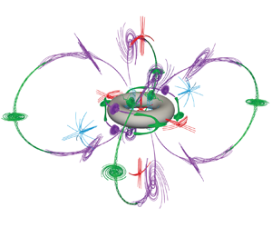
After investigating streaming flows in terms of body geometry and flow inertia variations, we finally begin to probe the effects of shape topological changes. The inextricable connection between topology and geometry provides a vast manipulation space that can hardly be systematically explored. Hence, here we narrow down the scope of our investigation and consider a single topological defect – a hole – in a spheroid similar to figure 4. We thus transition from a genus-0 spheroid (body with no holes) to a genus-1 torus (body with one hole) of comparable length scales. We then consider four representative  $\delta _{AC} / a$ values between the Stokes-like and the finite-thickness DC layer regimes, as shown in figure 6. This gives us the opportunity to begin to understand how flow structures pertinent to the spheroid remodel due to the interaction with the flow within the topological defect.

Figure 6. Streaming flow topology at different  $\delta _{AC} / a$ for a torus, with axis of symmetry aligned along the $z$-axis, oscillating along the $x$-axis. The torus has tube radius $a_{tube} = 0.25 a$ and core radius $a_{core} = 0.75 a$, so that the overall body length scale is $a = a_{tube} + a_{core}$. We highlight here that the torus has major ( $a_{max} = a$) and minor ( $a_{min} = a_{tube} = 0.25 a$) length scales comparable to those of the 3-D spheroid in § 5, essentially presenting equivalent width and thickness. Simulation details: normalized uniform grid spacing $h / a = 0.03$.
When considering high  $\delta _{AC}/ a$, we encounter the streaming flow topology representative of the Stokes-like regime as depicted in figure 6(a). In this regime, we observe the presence of two rings, fit to the body and made of two stable (purple) and unstable (green) FSS connected by heteroclinic orbits, similar to those encountered in figure 4. These rings are unaffected by the topological defect. Indeed, due to the proximity to the body, the flow effectively detects only the object's outer curvature, which is similar to the spheroid. Within the topological defect, we observe a collection of critical points (one unstable NSS (red), two stable NSS (blue) and four unstable FSS (green) – inset). Additionally, a pair of stable NSS is found along the $z$-axis, off the $xy$-plane. This particular pair, as we will see, plays a significant role in remodelling the flow relative to the genus-0 spheroid. Indeed, it extends the influence zone of the topological defect, providing opportunities for structures exterior to the torus to eventually interact.
As we decrease  $\delta _{AC} / a$, we see an interesting mechanism play out. At first the flow exterior to the torus evolves in accordance to the spheroid case (Phase I $\rightarrow$ III), whereby two stable NSS approach from infinity along the $y$-axis, and then undergo a pitchfork bifurcation forming the unstable NSS (red) and pairs of stable FSS (purple), on both sides of the torus (figure 6b). This process is thus still governed by the object's outer curvature. Nonetheless, after the pitchfork bifurcation takes place, the pair of purple FSS progressively fans out in the $yz$-plane and approaches the defect's zone of influence, represented by the two stable NSS along the $z$-axis. The result of this interaction manifests in the first departure from the flow evolution depicted in figure 4. Indeed, the stable FSS (purple) now further bifurcate into a pair of stable FSS and an unstable NSS (figure 6c). We note that here we encounter again a two-step mechanism: first we have a supercritical pitchfork bifurcation (stable FSS $\rightarrow$ 2 stable FSS $+$ 1 unstable FSS) followed by a change in nature from FSS to NSS on the unstable branch. Concurrently, on the $xy$-plane we observe the appearance of the two unstable FSS (green) and stable NSS (blue) already seen in Phase III $\rightarrow$ V of the spheroid (figure 4, § 5.2). This is consistent with the intuition that external flow structures, especially in the $xy$-plane, are insensitive to the topological defect and primarily respond to the object's outer curvature. Overall, this process sets the stage for a dramatic reconfiguration of the finite-thickness regime, relative to the spheroid. Indeed, in the outer flow region, there are now eight stable and only four unstable FSS. Thus these critical points no longer have the opportunity to form the pair of outer rings (each made of two stable and two unstable FSS) of figure 4. Instead, they are forced to connect in a new structure capable of accommodating the four extra stable FSS. The solution is offered by a clover-like ring structure running through the midpoint of the topological defect (figure 6d). This meeting point also has the effect of ‘locking’ the rings in, preventing any further re-orientation, unlike those observed for the spheroid (Phases V and VI in figure 4). The resulting flow now fundamentally differs from previously observed finite-thickness regimes. In fact, although we can still identify a DC layer organized around the smaller rings fit to the body, this recirculating flow region is now confined by an outer flow that both extends to infinity and permeates the centre of the domain by merging through the hole of the torus. This unique configuration may offer novel microfluidic opportunities (subject to the considerations of § 3.2), whereby the easily accessible outer flow now provides a natural mechanism to transport particles from the top and bottom of the torus to the topological defect, thus focusing them for self-assembly or mixing applications.
7. Conclusion
Towards the goal of extending our understanding of streaming flow dynamics in 3-D settings, we start by revisiting the classical case of the oscillating sphere and present observed flow structures and transitions through the lens of dynamical systems theory (Bhosale et al. Reference Bhosale, Parthasarathy and Gazzola2020). We further demonstrate the utility and extensibility of this approach to understand streaming flows in more general, but still axisymmetric 3-D cases. We then systematically investigate streaming in a fully 3-D setting by oscillating a spheroid perpendicular to its axis of symmetry, revealing a rich dynamic behaviour that we understand using bifurcation theory. Finally, we present a first foray into streaming induced by a topologically distinct body. Thus a torus of length scales comparable with the previously investigated spheroid is analysed, revealing intriguing flow organizations of potential utility for microparticle concentration, self-assembly and mixing. Altogether, these results provide physical intuition, principles and analysis tools to manipulate 3-D streaming flows based on body geometry, topology and flow inertia, with potential applications in microfluidics and microrobotics.
Supplementary material
Supplementary material is available at https://doi.org/10.1017/jfm.2021.1106.
Acknowledgements
We thank S. Hilgenfeldt for helpful discussions over the course of this work.
Funding
The authors acknowledge support by the National Science Foundation under NSF CAREER grant no. CBET-1846752 (M.G.) and by the Blue Waters project (OCI-0725070, ACI-1238993), a joint effort of the University of Illinois at Urbana-Champaign and its National Center for Supercomputing Applications. This work also used the Extreme Science and Engineering Discovery Environment (XSEDE) (Towns et al. Reference Towns2014) Stampede2, supported by National Science Foundation grant no. ACI-1548562, at the Texas Advanced Computing Center (TACC) through allocation TG-MCB190004.
Declaration of interests
The authors report no conflict of interest.


 Open access