


1. Introduction
In turbulent wall-bounded shear flows, only the mean flow is energised by external driving effects and so it has to pass on some of its energy to the fluctuation field. Linearising the Navier–Stokes equations around the mean velocity profile is sufficient to capture all the possible energy transfer processes. Hence, linear models based on modal stability analysis or transient growth are popular tools used in flow control (Kim & Bewley Reference Kim and Bewley2007; Rowley & Dawson Reference Rowley and Dawson2017). Recently, in a comprehensive cause-and-effect study, Lozano-Duran et al. (Reference Lozano-Duran, Constantinou, Nikolaidis and Karp2021) (hereafter LD21) identified that transient growth around the streamwise-averaged velocity profile is the essential linear mechanism needed to sustain turbulence in plane channel flow with a particular threshold of the growth required at  $Re_\tau =180$ in a minimal flow unit. This result hints at a possible and interesting update on Malkus's (Reference Malkus1956) well known but defunct hypothesis (e.g. Reynolds & Tiedermann Reference Reynolds and Tiedermann1967) that the turbulent mean profile $U(y)\hat {\boldsymbol {x}}$ (where $x$ is the streamwise direction and $y$ the cross-shear direction) is marginally (linearly) stable. Instead, the result of LD21 suggests that there may be some sort of statistical (linear) transient growth threshold on the extended mean profiles ${\mathcal {U}}(y,z,t)\hat {\boldsymbol {x}}$ (where $z$ is the spanwise direction) realised in the flow (‘statistical’ here means in some averaged sense over the family of realised profiles ${\mathcal {U}}(y,z,t)$ parametrised by time $t$ rather than ‘statistical stability’ ideas considered in Markeviciute & Kerswell (Reference Markeviciute and Kerswell2023)). An alternative perspective is that the mean $U(y)\hat {\boldsymbol {x}}$ has a threshold for nonlinear transient growth where the growth possible for perturbations of a finite amplitude have to be considered (‘finite’ because the streak field is generated as part of the growth). The work of LD21 needs extending, however, to larger flow domains to test robustness and higher $Re_\tau$ to reveal how the threshold growth possibly scales. Unfortunately, the amount of computation involved is forbidding, which suggests trying to identify and study a theoretical proxy. So motivated, we build a simple two-stage model of primary and secondary linear transient growth here and use this to suggest how LD21's results would generalise. The primary linear process is the energy transfer from the streamwise- and spanwise-averaged velocity profile $U(y)\hat {\boldsymbol {x}}$ via streamwise rolls to spanwise-dependent but streamwise-independent streaks $\boldsymbol {\mathcal {U}}(y,z,t)\hat {\boldsymbol {x}}$ due to the non-normality of the linear operator. This transient growth process is now well understood (e.g. Orr (Reference Orr1907) and Farrell (Reference Farrell1988) for laminar flows; Kim & Lim (Reference Kim and Lim2000), del Alamo & Jimenez (Reference del Alamo and Jimenez2006) and Cossu, Pujals & Depardon (Reference Cossu, Pujals and Depardon2009) in turbulent settings). The streak formation can also be explained through a stable mode in statistically forced turbulence modelled with statistical state dynamics (Farrell, Ioannou & Nikolaidis Reference Farrell, Ioannou and Nikolaidis2017), or by the pattern-forming properties of the lift-up, shear and diffusion of the mean profile (Chernyshenko & Baig Reference Chernyshenko and Baig2005). Most notably, Butler & Farrell (Reference Butler and Farrell1993) were able to show that the observed spanwise streak spacing was consistent with optimal disturbances constrained to grow maximally over an eddy turnover time.
Taking the new base flow as the final primary streak structure added to the mean velocity profile, the secondary linear process can be considered to model the subsequent streak breakdown. The exact linear mechanism driving the breakdown has been widely discussed. While some studies emphasised the importance of the modal instability of the streaks (Hamilton, Kim & Waleffe Reference Hamilton, Kim and Waleffe1995; Andersson et al. Reference Andersson, Brandt, Bottaro and Henningson2001), Schoppa & Hussain (Reference Schoppa and Hussain2002) showed that most of the streaks observed in simulations are in fact exponentially stable and suggested transient growth as the driving mechanism of streak breakdown. The feasibility of this conclusion was debated (Jiménez Reference Jiménez2018) and alternative explanations such as parametric streak instability considered (Farrell & Ioannou Reference Farrell and Ioannou1999; Farrell et al. Reference Farrell, Ioannou, Jiménez, Constantinou, Lozano-Durán and Nikolaidis2016). Recently, in their exhaustive cause-and-effect study of possible secondary linear mechanisms, LD21 showed that transient growth fuelled by ‘push-over’ and Orr mechanisms (Orr Reference Orr1907) is the necessary ingredient in sustaining turbulence in minimal channels at least at  $Re_\tau =180$. However, it remains unknown what perturbations and primary streak amplitudes lead to transient growth levels sufficient to sustain turbulence, the understanding of which could enhance flow control strategies. Previous work in this direction is mainly direct numerical simulations (DNS)-based including the direct-adjoint looping optimisation of the nonlinear Navier–Stokes equations around a laminar Poiseuille profile with varying amplitude streak (Cossu, Chevalier & Henningson Reference Cossu, Chevalier and Henningson2007).
In this paper we examine a two-stage transient growth process to study the optimal perturbation energy gain starting from a  $U(y)\hat {\boldsymbol {x}}$ mean flow generated by DNS in a minimal channel. A (primary) transient growth calculation is then performed in the same spirit as Butler & Farrell (Reference Butler and Farrell1993) which seeks the maximal streak produced over the local eddy turnover time $T$, viz.
 \begin{equation} \text{primary growth} \quad U(y)\hat{\boldsymbol{x}} +\varepsilon \tilde{\boldsymbol{u}}(y,z,0) \xrightarrow{\max _{\tilde{\boldsymbol{u}}(y,z,0)} E_p} U(y)\hat{\boldsymbol{x}}+\varepsilon \tilde{\boldsymbol{u}}(y,z,T), \end{equation}
where  $E_p:= \int _V \tilde {\boldsymbol {u}}(y,z,T)^2 \,{\rm d}^3 \boldsymbol {x}$ and $\int _V \tilde {\boldsymbol {u}}(y,z,0)^2 \,{\rm d}^3 \boldsymbol {x}=1$ and $\varepsilon \rightarrow 0$ is assumed. This selects a unique streak structure $\tilde {\boldsymbol {u}}(y,z,T)$ but not an amplitude since only $O(\varepsilon )$ terms are retained. We then examine the (secondary) transient growth possible on a new base flow of mean plus frozen, final streak field across an array of streak amplitudes $A$ – i.e. ${\mathcal {U}}(y,z;A):= U(y) \hat {\boldsymbol {x}}+A\tilde {\boldsymbol {u}}(y,z,t_p)$ – as a function of $t$ (see expression given in (2.10) below), viz.
 \begin{align} \text{secondary growth} \quad {\mathcal{U}}(y,z;A)\hat{\boldsymbol{x}} +\varepsilon \check{\boldsymbol{u}}(x,y,z,0) \xrightarrow{\max_{\check{\boldsymbol{u}}(x,y,z,0)} E_s} {\mathcal{U}}(y,z;A)\hat{\boldsymbol{x}}+\varepsilon \check{\boldsymbol{u}}(x,y,z,t), \end{align}
where  $E_s:= \int _V \check {\boldsymbol {u}}(x,y,z,t)^2 \,{\rm d}^3 \boldsymbol {x}$ and $\int _V \check {\boldsymbol {u}}(x,y,z,0)^2 \,{\rm d}^3 \boldsymbol {x}=1$. This simple process is found to capture transient growth of the perturbations consistent with observations in LD21 at $Re_\tau =180$ when streak amplitudes seen in the DNS and the appropriate time horizon are used. We then exploit this correspondence to predict what sort of transient growth can be achieved in larger channels and higher Reynolds numbers.
2. Problem set-up
2.1. Mean velocity profile
To obtain the mean velocity profile for the primary transient growth calculations, either DNS were performed in the minimal channel flow unit (Jiménez & Moin Reference Jiménez and Moin1991) using the DNS code Dedalus (Burns et al. Reference Burns, Vasil, Oishi, Lecoanet and Brown2020) or data was imported from the large channel turbulent runs of Lee & Moser (Reference Lee and Moser2015) (hereafter LM15).
The streamwise, wall-normal and spanwise directions of the channel are labelled as  $x,y$ and $z$, respectively, with corresponding velocity fields $u,v,w$ and pressure $p$. Variables are non-dimensionalised by the channel half-height $h$ and the average wall shear velocity $u_{\tau }$, which together with kinematic viscosity $\nu$ define the Reynolds number
 \begin{equation} Re_{\tau} := u_{\tau}h/\nu \end{equation}
and a time unit  $h/u_\tau$. The incompressible Navier–Stokes equations are then
 $$\begin{gather} \frac{\partial \boldsymbol{u}}{\partial t} + \boldsymbol{u} \boldsymbol{\cdot} \boldsymbol{\nabla} \boldsymbol{u} =-\boldsymbol{\nabla} p + \frac{1}{Re_{\tau}} \nabla^2 \boldsymbol{u} +\hat{\boldsymbol{x}}, \end{gather}$$
 $$\begin{gather}\boldsymbol{\nabla} \boldsymbol{\cdot} \boldsymbol{u} =0, \end{gather}$$
with an imposed streamwise pressure gradient  $-\boldsymbol {\nabla } P = \hat {\boldsymbol {x}}$. The same minimal flow domain, $(L_x^+,L_y^+,L_z^+)=(337,2Re_{\tau },168)$ (the superscript ‘+’ indicates relative to viscous length units of $\nu /u_{\tau }$ or viscous time units of $\nu /u_\tau ^2$) is used as in LD21. No-slip boundary conditions were imposed at the channel walls located at $y=\pm 1$ and periodicity imposed in the streamwise and spanwise directions. Discretisation was through a triple Fourier–Chebyshev–Fourier expansion in $x,y$ and $z$, respectively, in Dedalus. For the minimal channel, the mean velocity profile $U(y)$ was obtained by averaging over the interval $[T_0,T_0+T]$ with $T_0>0$ chosen to avoid initial transients and is shown for $Re_\tau =180$, 360 and 720 in figure 1. Also shown are the mean profiles from the ‘large’ channel runs of LM15 where $(L_x,L_y,L_z)=(8 {\rm \pi},2,3 {\rm \pi})$. They agree well up to at least $y^+ \approx 50$ consistent with the estimate $0.3L_z^+$ given by Flores & Jiménez (Reference Flores and Jiménez2010) and so well above $y^+ \approx 18$ where the primary streaks are found to be located. The outputs of the simulations were checked by using different resolutions, e.g. $N_y=90$ and $N_y = 180$ for $Re_{\tau } = 360$, $N_y=180$ and $N_y = 256$ for $Re_{\tau } = 720$ (LD21 used second-order finite differences across half the channel for their calculations and $T=300$).

Figure 1. Plot of  $U^+(y^+)$ (black, red and blue solid lines for minimal channels at $Re_\tau =180$, 360 and $720$, respectively; magenta and green dotted lines for LM15 channels at $Re_\tau =180$ and $550$, respectively). The primary streak profiles $A \tilde {u}_{n_p}(y;t_p)$ (see expression (2.10) below) with $n_p=1$ or $\lambda _z^{p+}=168$ for the minimal and $\lambda _z^{p+} = 154 (136)$ for the large channels at $Re_{\tau } = 180 (550)$, respectively, are shown using dashed lines and the corresponding colours with $A=10 / \sqrt {Re_{\tau }}$ to highlight their similarity ( $\tilde {u}_{n_p}(y;t_p)$ is normalised to have the same amplitude as $U$, which scales with $\sqrt {Re_\tau }$ in viscous units). The primary streaks are all peaked at $y^+ \approx 18$ consistent with the findings of Butler & Farrell (Reference Butler and Farrell1993).
2.2. Primary transient growth
We consider primary transient growth of streamwise-independent perturbations to the mean velocity profile  $U(y)$ defined as $[{\tilde {u}},{\tilde {v}},{\tilde {w}}] = [u-U,v,w]$ and decomposed into spanwise Fourier modes as follows:
 \begin{equation} [\tilde{\boldsymbol{u}}(y,z,t), {\tilde{p}}(y,z,t) ] = \sum_{n} [\tilde{\boldsymbol{u}}_{n}(y,t), \tilde{p}_{n}(y,t) ] \exp ({\rm i}n \beta z) + {\rm c.c.}, \end{equation}
where  $\beta :=2{\rm \pi} /L_z$. The linearised Navier–Stokes equations around the mean $U(y)\hat {\boldsymbol {x}}$ for each $n$ are
 \begin{equation} \partial_t \tilde{\boldsymbol{u}}_{n} + (\partial_y U) \tilde{v}_{n} \boldsymbol{\hat{x}} =- \boldsymbol{\nabla} \tilde{p}_{n} + \frac{1}{Re_{\tau}} \nabla^2 \tilde{\boldsymbol{u}}_{n} , \quad \boldsymbol{\nabla} \boldsymbol{\cdot} \tilde{\boldsymbol{u}}_{n} = 0, \end{equation}
and can be treated separately. Due to the non-normality of the linear operator, the perturbations can experience transient growth in energy quantified by the (primary) gain
 \begin{equation} G_p(n,t_p) := \sup_{\tilde{\boldsymbol{u}}_{n}(y,0)}\frac{\|\tilde{\boldsymbol{u}}_{n}(y,t_p)\|^2}{\|\tilde{\boldsymbol{u}}_n(y,0)\|^2}, \end{equation}
where the energy norm is calculated by
 \begin{equation} E_n := \|\tilde{\boldsymbol{u}}_{n}\|^2 = \int_{-1}^{1} |\tilde{u}_{n}|^2+|\tilde{v}_{n}|^2+|\tilde{w}_{n}|^2 \, {{\rm d}\kern0.05em y}. \end{equation}
The goal of the primary transient growth calculation is to identify the streamwise-independent streak field  $\tilde {u}_{n_p}(y;t_p) \exp ({\rm i} n_p \beta z)$ (with wavelength $\lambda _{z}^{p}:= 2{\rm \pi} /n_p \beta$) which achieves optimal energy growth at time $t_p$. This will then be used as the two-dimensional (2-D) streak field upon which to study secondary growth. Two issues require discussion: (i) how to choose $t_p$ (which then specifies the streak spacing) and (ii) what amplitude to make the streaks for the secondary growth analysis.
2.3. Time scale for primary transient growth
Choosing the primary transient growth time scale  $t_p$ presents a challenge as the global (over all $t_p$) optimal growth is achieved at a time much greater than the characteristic time scale of turbulent fluctuations by perturbations with larger than observed spanwise spacing. Butler & Farrell (Reference Butler and Farrell1993) realised that perturbations can only grow over the time limited by the eddy turnover time $t^+_e(y^+)=Re_{\tau } q^2(y^+)/\epsilon (y^+)$ (the ratio of the characteristic turbulent velocity squared $q^2$ and dissipation rate $\epsilon$ at a given distance $y^+$ from the wall, given in viscous units) before being disrupted by turbulent fluctuations. Butler & Farrell (Reference Butler and Farrell1993) suggested choosing $t^+_p=t^+_e(y^+_*)$ where $y^+_*$ is the unique wall distance where the optimal streak is positioned given a growth time equal to the local eddy turnover time. While such restriction of the primary transient growth time scale was debated by Waleffe & Kim (Reference Waleffe and Kim1997) and Chernyshenko & Baig (Reference Chernyshenko and Baig2005), it provides a practical approach to obtain realistic streamwise streak profiles and will be used below. To calculate the eddy turnover time we use the following definitions:
 $$\begin{gather} q^2(y):= \frac{1}{T L_z L_x } \int_{T_0}^{T_0+T} \int_0^{L_z} \int_0^{L_x} [ (u-U)^2 + v^2 + w^2 ] \, {{\rm d}\kern0.06em x} \, {\rm d}z \, {\rm d}t, \end{gather}$$
 $$\begin{gather}\epsilon(y) := \frac{1}{T L_z L_x } \int_{T_0}^{T_0+T} \int_0^{L_z} \int_0^{L_x} |\boldsymbol{\nabla}(\boldsymbol{u}-U\hat{\boldsymbol{x}})|^2\, {{\rm d}\kern0.06em x} \, {\rm d}z \, {\rm d}t. \end{gather}$$
Then, we compare the centre of the streak location (defined by maximum velocity) as a function of the streak optimisation time to the eddy turnover time  $t^+_e$ as a function of the distance from the wall $y^+$, plotted using viscous units in figure 2. The intersection points are at $t^+_p=114$, $97$ and $95$ for $Re_\tau =180$, 360 and $720$, respectively, in the minimal channel (giving a streak spacing of $\lambda _z^{p+}=168$) and at $t^+_p=79$ and $t^+_p=89$ in the large channel for $Re_\tau =180$ and $550$, respectively (giving streak spacing of $\lambda _z^{p+}=106$ and $\lambda _z^{p+}=112$, respectively), see table 1.

Figure 2. Eddy turnover time  $t^+_e=Re_{\tau } q^2/\epsilon$ (black, red and blue lines for $Re_\tau =180$, 360 and $720$, respectively; magenta and green lines for $Re^{LM15}_\tau =180$ and $550$, respectively). The location of the optimal streak as a function of the optimisation time is shown as thin black curves for the minimal channel (left) and the large channel (right) (the kink in the curve is due to the discrete change in optimal spanwise wavenumber of the streak). Chosen primary transient growth time horizons are marked with dotted lines. See table 1 for numerical values of $t_e^+$ at the various $Re_\tau$.
Table 1. Parameters for the different cases considered. At the top are the results for the minimal box simulations and at the bottom are the results using data from Lee & Moser (Reference Lee and Moser2015). Here  $N_y$ is the wall-normal Chebyshev resolution used in transient growth calculations, $\lambda _x^+$ and $\lambda _z^+$ are the largest streamwise and spanwise wavelengths present, $\lambda _z^{p+}$ is the primary streak spacing and $t^+_e$ is the estimated eddy-turnover time. Here $y^+_*$ is the unique distance from the wall at a given $Re_\tau$ where the optimal streak has a maximal growth time equal to the local eddy turnover time.

2.4. Amplitude for the primary streak
For the secondary transient growth calculation, the streamwise-independent base flow is defined as
 \begin{equation} {\mathcal{U}}(y,z) \hat{\boldsymbol{x}} := U(y)\hat{\boldsymbol{x}} + [A {\tilde{u}}_{n_p}(y;t_p) \exp (2 {\rm \pi}{\rm i} z/\lambda_z^p ) +{\rm c.c.}]\hat{\boldsymbol{x}} \end{equation}
with normalisation  $\|\tilde {u}_{n_p}(y;t_p)\|^2=\|U\|^2$ (the ${\tilde {v}}_{n_p}$ component is not used). The (non-dimensional) primary streak amplitude $A$ is then the amplitude of the Fourier mode corresponding to the streak normalised by that corresponding to the mean flow. This ratio was deduced directly from time-averaging DNS data in the minimal channel or via the DNS data reported by LM15 for the larger channel. Without loss of generality, the streak field is chosen to be symmetric about $z=0$ and then ${\tilde {u}}_{n_p}(y;t_p)$ is real. In what follows, the mean amplitude, $\bar {A}$, and standard deviation, $A_\sigma$, were collected for the minimal channel whereas only $\bar {A}$ was available for the large channel (see table 1).
2.5. Secondary transient growth
Secondary transient growth perturbations are superimposed on the streak field  ${\mathcal {U}}$ given in (2.10) so that $\check {\boldsymbol {u}}=[{\check {u}},{\check {v}},{\check {w}}] = [u-{\mathcal {U}},v,w]$ where $\check {\boldsymbol {u}}$ is assumed infinitesimally small. The secondary perturbation is decomposed into Fourier modes,
 \begin{equation} [\check{\boldsymbol{u}}(x,y,z,t), \check{p}(x,y,z,t) ] = \sum_{m} [\check{\boldsymbol{u}}^{m}(y,z,t), \check{p}^{m}(y,z,t) ] \exp{({\rm i} m \alpha x)}, \end{equation}
where
 \begin{equation} [\check{\boldsymbol{u}}^{m}(y,z,t), \check{p}^{m}(y,z,t) ] = \sum^N_{n =-N} [\check{\boldsymbol{u}}^{m}_{n}(y,t), \check{p}^{m}_{n}(y,t) ] \exp{(2 {\rm \pi}{\rm i}(\mu+n) z/\lambda_z^{p} )}, \end{equation}
so  $\mu \in [0,\tfrac {1}{2}]$ is a ‘modulation’ parameter and $\alpha :=2{\rm \pi} /L_x$. The secondary disturbance only has the same spanwise wavelength as the streak field when $\mu =0$ (no modulation) otherwise the spanwise wavelength of the secondary perturbation increases by a factor $1/\mu$ over that of the primary perturbation. Hereafter we just consider $\mu =0$ so the growths found below are a lower bound on what is possible across all $\mu$.
In the linearised equations determining how  $\check {\boldsymbol {u}}$ evolves, the Fourier modes in $x$ can be treated separately but the spanwise wavenumbers are coupled by the streak field adding new terms to the linearised equations (2.5):
 \begin{gather} \partial_t \check{\boldsymbol{u}}^{m}_{n} + \overbrace{{\rm i} m \alpha [U \check{\boldsymbol{u}}^{m}_{n} + A {\tilde{u}}_{n_p} \check{\boldsymbol{u}}^{m}_{n-1} + A {\tilde{u}}_{n_p}^{*} \check{\boldsymbol{u}}^{m}_{n+1}]}^{\mathit{advection}} +\overbrace{(\partial_y U) {\check{v}}^{m}_{n}\boldsymbol{\hat{x}}}^{\mathit{lift\text-up}} \nonumber\\ \qquad +\underbrace{A[ \partial_y {\tilde{u}}_{n_p} {\check{v}}^{m}_{n-1} + \partial_y {\tilde{u}}_{n_p}^{*} {\check{v}}^{m}_{n+1} ] \boldsymbol{\hat{x}}}_{\mathit{extra \ lift\text-up}} +\underbrace{\frac{2{\rm \pi} {\rm i}}{\lambda_z^p} A [{\tilde{u}}_{n_p} {\check{w}}^{m}_{n-1} -{\tilde{u}}_{n_p}^{*} {\check{w}}^{m}_{n+1}]\hat{\boldsymbol{x}}}_{\mathit{push\text-over}}\nonumber\\ =-\left( \begin{array}{@{}c@{}} {\rm i} m \alpha \\ \partial_y \\ 2 {\rm \pi}{\rm i} n/\lambda_z^p \end{array}\right) \check{p}^{m}_{n} +\frac{1}{Re_{\tau}}\left[\partial_y^2-m^2 \alpha^2 -\frac{4 {\rm \pi}^2 n^2}{(\lambda_z^{p})^2} \right]\check{\boldsymbol{u}}^{m}_{n}, \end{gather}
 \begin{gather} {\rm i}m\alpha {\check{u}}^{m}_{n}+\partial_y {\check{v}}^{m}_{n} +\frac{2 {\rm \pi}{\rm i} n }{\lambda_z^p} {\check{w}}^{m}_{n}=0. \end{gather}
We solve equations (2.13)–(2.14) for each value of  $m$ (or equivalently wavelength $\lambda _x=2{\rm \pi} /m \alpha =L_x/m$) separately while $2N_z+1$ spanwise modes are coupled using $n \in [-N_z,N_z]$. The definition of the secondary gain is
 \begin{equation} G^m_s(t_s;\lambda_z^{p+},A,Re_{\tau}) := \sup_{\check{\boldsymbol{u}}^{m}(y,0)}\frac{\|\check{\boldsymbol{u}}^{m}(y,z,t_s)\|^2}{\|\check{\boldsymbol{u}}^{m}(y,z,0)\|^2} \end{equation}
and
 \begin{equation} G_s(t_s;\lambda_z^{p+},A,Re_{\tau}):= \max_{m}G^m_s(t_s;\lambda_z^{p+},A,Re_{\tau}) \end{equation}
is the optimal gain across the set of wavenumbers considered (and  $\mu =0$). We explore how this optimal gain changes as the primary streak amplitude $A$ is increased over the range of values observed in the simulations.
2.6. Numerical implementation
To perform the primary and secondary transient growth calculations, we follow the matrix-algebra approach described in Reddy & Henningson (Reference Reddy and Henningson1993). If  $\boldsymbol {q}_j=(u_j,v_j,w_j,p_j)$ is the $j$th eigenfunction corresponding to the eigenvalue $\lambda _j$ and ordered by increasing damping rate $-\Re e(\lambda _j)$, then Reddy & Henningson (Reference Reddy and Henningson1993) define the eigenvalue ‘overlap’ matrix as
 \begin{equation} {\mathsf{C}}_{jk} := \langle \boldsymbol{q}_j, \boldsymbol{q}_k \rangle:= \int \int_{-1}^{1} \int u_j^*u_k+v_j^*v_k+w_j^* w_k\, {{\rm d}\kern0.06em x}\, {{\rm d}\kern0.05em y} \,{\rm d}z, \end{equation}
where the inner product is that induced by the energy norm defined in (2.7), the integration is over a wavelength in  $x$ and $z$, and $^*$ indicates complex conjugation. This matrix is diagonal if the eigenfunctions form an orthonormal set but, as is typical for shear flow problems, is dense here. It is, however, Hermitian and positive definite which means there exists a matrix $\boldsymbol{\mathsf{F}}$ such that $\boldsymbol{\mathsf{C}}=\boldsymbol{\mathsf{F}}^{\boldsymbol {H}} \boldsymbol{\mathsf{F}}$ where $\boldsymbol{\mathsf{F}}^{\boldsymbol {H}}:=(\boldsymbol{\mathsf{F}}^*)^T$ is its Hermitian conjugate ( $\boldsymbol{\mathsf{F}}$ is found using the singular value decomposition of $\boldsymbol{\mathsf{C}}=\boldsymbol {U}{\boldsymbol {\varSigma }} \boldsymbol {V^H}$ so that $\boldsymbol{\mathsf{F}}:= \boldsymbol {U} \sqrt {\boldsymbol {\varSigma }}\boldsymbol {V^H}$, where $\sqrt {\boldsymbol {\varSigma }}$ indicates a diagonal matrix with the square root of $\boldsymbol{\mathsf{C}}$'s singular values on the diagonal). Then the largest growth can be computed by squaring the largest singular value of $\boldsymbol{\mathsf{F}} \,{\rm e}^{t \boldsymbol {\Lambda }} \boldsymbol{\mathsf{F}}^{-1}$, where ${\rm e}^{t\boldsymbol {\Lambda }}$ is the diagonal matrix exponential with ${\rm e}^{t\lambda _j}$ on the diagonal (see equation (30) in Reddy & Henningson (Reference Reddy and Henningson1993)).
The symmetry in the wall-normal direction allows disturbances satisfying the symmetries
 \begin{equation} Z_-:(u,v,w,p)(x,y,z,t) \to (u,-v,w,p)(x,-y,z,t) \end{equation}
and
 \begin{equation} Z_+:(u,v,w,p)(x,y,z,t) \to (-u,v,-w,-p)(x,-y,z,t), \end{equation}
to be considered separately. Discretisation of the linear operators corresponding to (2.5) and (2.13)–(2.14) produce matrices of size  $2N_y$ and $2N_y(2N_z+1)$, respectively. For the primary transient growth calculation, $N_e=80$ eigenfunctions were used in the expansion which was tested by accurately reproducing the results in Butler & Farrell (Reference Butler and Farrell1993) who used a modelled mean profile. Optimal streaks located near the wall were found to be the same for $Z_-$ and $Z_+$, and so the primary streak profile was chosen with $Z_-$ symmetry. No change in the optimal streaks were observed repeating the calculation with double the wall-normal resolution.
For the secondary transient growth calculation, a spanwise truncation of  $N_z = 8$ proved adequate typically giving a spectral drop off of over six orders of magnitude in the output mode, see figure 3 which compares $N_z=8$, $12$ and $16$. The choice of appropriate $N_e$ is more delicate with increasing values needed for smaller $\lambda _x$ and short times. Typically $N_e=500\unicode{x2013}800$ was used as a compromise between accuracy and runtimes. In all cases, secondary perturbations with $Z_-$ symmetry yielded dominant transient growth values and are presented in this paper.

Figure 3. Energy distribution over spanwise wavenumbers  $n$ for the optimal secondary transient growth mode at $\lambda _x=L_x$ and $Re_\tau =180$ in the minimal channel with primary streak $\lambda _z^{p+}=168$ and amplitude $\bar {A}$. Shown for $N_z = 8,12$ and $16$ using black solid, dotted and dashed lines for the input modes (respectively), and red crosses, circles and a solid line (respectively) for the output modes. This figure indicates that even for $N_z=8$, there is a spectral drop off in energy of six orders of magnitude for the output modes.
3. Results
3.1. Two-stage optimisation
We first consider the minimal domain and  $Re_{\tau }=180$ used by LD21. The approach taken here is to do two optimisations in sequence to estimate the energy growth possible in the flow over time scales consistent with the eddy turnover times near the wall. The first optimisation is used to define the streak field using linear transient growth analysis and the second optimisation then finds the optimal secondary growth on the primary streak field once it has been given an amplitude. This is admittedly a simplistic approach which relies on a time scale separation argument that the secondary growth occurs over a shorter time scale than the evolution of the streaks so they can be considered steady. This is unlikely to be true but the alternatives (discussed later) require a significantly more complex approach. Given this, trying this simple and interpretable approach to see if it captures the sort of growths found by LD21 seemed reasonable.
The first optimisation has already been discussed with the result that a primary streak of spanwise spacing  $\lambda _z^{p+}=168$ – the largest spanwise streak which fits into the minimal box – emerges using the approach advocated by Butler & Farrell (Reference Butler and Farrell1993). Reassuringly, this is the most energetic streak seen in our simulations consistent with LD21 (see their figures 2 and 3) followed by the $\lambda _z^+=84$ double streak (both can be seen in the simulations, see figure 4). The results of the secondary optimal gain
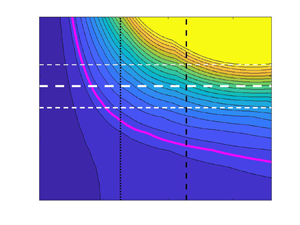
  $G_s(t_s^+;168,A,Re_{\tau })$ contoured over the $(t_s^+, A \sqrt {Re_{\tau }})$ plane are shown in figure 5 with the associated optimising streamwise wavenumber index $m$ shown on the right-hand axis ( $A$ is multiplied by $\sqrt {Re_{\tau }}$ to bring it into alignment with $U$ which scales with this factor in viscous units). Figure 5(a,b) shows the results of restricting the optimisation to integer $m$, that is, secondary disturbances which fit into the minimal box. This shows two distinct regions where the secondary growth optimal is 2-D ( $m=0$) and where the optimal is 3-D (always corresponding to $m=1$ so the streak just streamwise-fits into the box). Interestingly, for amplitudes of the primary streak seen $A \in [\bar {A}-A_\sigma,\bar {A}+A_\sigma ]$ and times around that quoted by LD21, $t_s^+=t_{LD21}^+:=63$ ( $=0.35h/u_\tau$ in their figure 9), the secondary mode is 3-D. In their § 6.3, LD21 also discuss a threshold of $G_s=50$ for sustainable turbulence (although their figure 22 actually suggests the threshold is closer to 40 than 50). This contour is highlighted in figure 5 and is clearly shown to thread the region of interest. Secondary growths exceeding this threshold dominate this region. In particular,
 \begin{equation} G_s(t_{LD21}^+;168,\bar{A},180) \approx 90, \end{equation}
with the growth ranging from 60 at  $A=\bar {A}-A_\sigma$ to 130 for $A=\bar {A}+A_\sigma$.

Figure 4. Sample snapshots of the  $x$-averaged velocity field $U^+(y^+,z^+)$ from a $Re_{\tau }=180$ simulation in the minimal channel of LD21. (a) Streaks with $\lambda ^{p+}_z=168$ ( $n_p=1$) and (b) streaks with $\lambda ^{p+}_z=84$ ( $n_p=2$). These figures show that both are visible at different times in the simulations.

Figure 5. (a) Secondary transient growth  $G_s(t_s^+;168,A,Re_{\tau }=180)$ contour plots over the $(t_s^+,A\sqrt {Re_{\tau }})$ plane. Contour increments are 20. (b) Corresponding optimal streamwise wavenumber $\alpha m_{max} = 2 {\rm \pi}/\lambda _x^+$, where green (blue) area corresponds to $m=1$ ( $m=0$) wavenumber, showing the existence of a region where three-dimensional (3-D) perturbations become optimal. Panels (c) and (d) show the same quantities, but calculated for the set $m \in \{0,0.2,\ldots,2\}$. In all four plots, the white long dashed line shows $\bar {A}$ for the streaks with standard deviations are indicated by short dashed lines (both from DNS). Time horizons $t_{LD21}^+=63$ and $t_e^+$ are marked with vertical black dotted and dashed lines, respectively, and a magenta (a,c) or red (b,d) solid contour show the $G_s((\lambda _x^+)_{\max })=50$ threshold.
Figure 5(c,d) extends the optimisation over longer streamwise wavenumbers (smaller  $m$) to clarify the 2-D–3-D transition: the optimal disturbances become progressively longer in streamwise wavelength as the optimisation time increases whereas at short times there is a sudden transition from infinite streamwise wavelength (i.e. 2-D) disturbances to those of short wavelength.
Figure 6 illustrates a typical secondary optimal example at streamwise wavenumber  $m=1$ ( $\lambda _x^+=337$). The initial state of the optimal is shown in figure 6(a–c) and the final evolved state in figure 6(d–f). Similar to the optimal modes found around the laminar velocity profile with a spanwise streak (Cossu et al. Reference Cossu, Chevalier and Henningson2007), the optimal modes are tilted upstream at the start of the process (flow is from right to left) and are then tilted downstream at the time of the maximum energy gain, with the wall-normal velocity component almost perpendicular to the wall. This is indicative of the Orr mechanism.

Figure 6. Optimal secondary transient growth modes with  $\lambda _x^+=337$ at $Re_{\tau }=180$, primary streak amplitude $A=\bar {A}$ and $t_e$. Shown for minimal channel streaks with $\lambda ^+_z=168$. Optimal input velocities are shown in panels (a–c) and optimal output velocities are shown in panels (d–f). The blue and yellow isosurfaces show $\pm 0.2$ of the maximum of each velocity component. The Orr mechanism is noticeable in wall-normal velocity component where the structures become perpendicular to the wall. Note, the wall is located vertically on the page at $y^+=0$ with the other at $y^+=2Re_\tau =360$, and the mean flow direction is from right to left.
A key finding from LD21 (see their § 6.4) is that the ‘lift-up’ mechanism is not important for the growth they observe but the ‘push-over’ (see equation (6.24) in LD21) and Orr mechanisms are. To test this in our calculations, we consider the growth for the specific case of  $m=1$ ( $\lambda _x^+=337$) which just fits in the minimal channel and so was considered by LD21, and suppress either the lift-up or push-over mechanisms in turn, see figure 7. With both present, the growth can range from 30 to 175 as the streak amplitude increases from $\bar {A}-2\sigma$ to $\bar {A}+2\sigma$ and the maximum growth at $A=\bar {A}$ is observed just beyond $t^+_{LD21}=63$. These results are in good agreement with LD21 where energy gains of the frozen-in-time-streak field reach $O(100)$ (see discussion surrounding their figure 9). Further agreement with LD21 is found when considering the effect of lift-up and push-over mechanisms on the optimal gain values. While excluding the lift-up mechanism maintains the same sort of secondary transient growth factors, excluding the push-over mechanism causes the maximum optimal gain to collapse to $G_s\lesssim 25$ independent of the streak amplitude and decreasing the optimal time scale to just $t^+_s=36$ (the same effect was also seen in the larger channel to be discussed in § 3.3). We thus also find that the ‘push-over’ mechanism is essential to obtain sufficient levels of transient growth needed to sustain turbulence whereas the lift-up mechanism is not.

Figure 7. Secondary transient growth of perturbations with  $\lambda _x=L_x$ ( $m=1$) at $Re_{\tau } = 180$ for $\lambda _z^+=168$. Energy gain $G_s(t_s;A,180)$ is shown for different primary streak amplitudes $A=[\bar {A},\bar {A}\pm \sigma,\bar {A}\pm 2\sigma ]$ (solid black, solid dark blue and dashed orange lines) and found (a) with full linear mechanism (b) excluding ‘lift-up’ (c) excluding ‘push-over.’ Dotted vertical lines show $t^+_{LD21} = 63$ time horizon while dashed vertical lines show the eddy turnover time $t^+_s = t^+_e$.
The conclusion of this section is then that a simplistic two-stage optimisation procedure is able to capture both the levels of growth found by LD21 in their DNS and the importance/unimportance of the push-over/lift-up mechanism in this. In fact, one could perhaps argue that too much growth is available through this simplistic approach. These are maximums, however, rather than expected values given generic, non-optimal initial secondary perturbations (a point well made recently in Frame & Towne (Reference Frame and Towne2023)). The questions now are (i) how do the possible growths vary with  $Re_{\tau }$, and (ii) how do things change with a larger channel? In the latter, for example, it is unlikely that the most energetic streak will be that with the largest spacing which fits into a larger domain.
3.2. Higher  $Re_{\tau }$

To explore higher  $Re_{\tau }$ without changing the domain, the two-stage optimisation procedure was repeated at $Re_{\tau }=360$ and $Re_{\tau }=720$ in the minimal channel. The optimal primary streak remains $\lambda _z^{p+}=168$ and the corresponding contour plots of the optimal transient growth on the $(t_s^+,A\sqrt {Re_{\tau }})$ plane are shown in figure 8 for relevant primary streak amplitudes observed in the simulations. Qualitatively, the plot remains largely unchanged when $Re_{\tau }$ is increased: the observed mean streak amplitude and $t_e^+$ both decrease but the secondary growth remains similar. In particular
 \begin{equation} G_s(t_{LD21}^+;168,\bar{A},720) \approx 90, \end{equation}
where  $m_{max}=1$ over integer values of $m$. Again the $G_s = 50$ contour threads the region around $(t_{LD21}^+,\bar {A}\sqrt {Re_\tau })$ with the main change being that the contours become steeper for increasing $Re_\tau$.

Figure 8. Secondary growth  $G_s$ at $Re_{\tau }=360$ (a) and $Re_{\tau }=720$ (b) for the optimal streak $\lambda _z^{p+}=168$. Time horizons $t_{LD21}^+$ and $t_e^+$ are marked with vertical black dotted and dashed lines, respectively. Horizontal white dashed lines show $\bar {A}\sqrt {Re_{\tau }}$ and $(\bar {A}\pm \sigma )\sqrt {Re_{\tau }}$. Magenta solid contour shows the $G_s=50$ threshold and contour levels have $\Delta G_s =20$.
3.3. Larger geometry
Here, we use the DNS data from the larger channel studied in LM15 (see table 1 for details) to investigate the presence of larger length scales in the two-stage optimisation procedure (e.g. the larger channel is over an order of magnitude wider). The mean profiles shown in figure 1(a) are fairly similar for  $Re_{\tau }=180$ (black solid line versus magenta dotted line) but, as expected, start to deviate going towards the centre of the channel for higher $Re_{\tau }$; compare the profile at $Re_{\tau }=550$ for the larger channel (green dotted line) with the minimal channel profile at $Re_{\tau }=720$ (blue solid line). Relative to the minimal channel, the eddy turnover time function $t_e^+(y^+)$ intersects with the optimal streak function at a streak position slightly farther from the wall and at a reduced turnover time $t_e^+(y^+_*)$ of 79 for $Re_{\tau }=180$ and 89 for $Re_{\tau }=550$, see figure 2. As a consequence, the resulting optimal primary streaks while similar in structure (upper plot in figure 1) differ in spanwise wavelength: $\lambda _z^{p+}=106$ and 112 in the larger channel (so closer to the observed peak spacing of 100 (Kline et al. Reference Kline, Reynolds, Schraub and Runstadler1967)) for $Re_{\tau }=180$ and 550, respectively, as opposed to $168$ in the minimal channel.
The large channel, however, does show an interesting new feature compared with the minimal channel: the primary streak which produces the most secondary growth over all streaks of the same amplitude is not the streak of largest amplitude seen in the DNS (the streak energy was computed by integrating up to  $y^+ \approx 18$ to focus on the near-wall structures). In fact adjusting for this difference in amplitude, the most energetic observed streak produces the most growth on account of its enhanced amplitude. At $Re_\tau =180$, the optimal (at fixed amplitude) primary streak has $\lambda _z^+=106$ whereas the largest observed amplitude streak has $\lambda _z^+=154$. This latter most energetic streak spacing is essentially the same as that found in the minimal channel once the exact geometries are taken into account (in this larger channel, $\lambda _z^+=154$ has 11 wavelengths in the domain as opposed to $\lambda _z^+=169.6$ which has 10). Figure 9 shows the optimal secondary growth over the $(t_s^+,A \sqrt {Re_{\tau }})$ plane for both. The contour plots look very similar to the minimal channel results in figure 5 with comparable growth possible, e.g.
 \begin{equation} G_s(t_e^+;106,\bar{A}_{106},180) \approx 60 \quad \text{and} \quad G_s(t_e^+;154,\bar{A}_{154},180) \approx 100. \end{equation}
Here a subscript on  $\bar {A}$ is now used to identify the streak wavelength and the eddy turnover time assumed for comparison purposes instead of $t^+_{LD21}$ which is only relevant for the minimal box. At $Re_{\tau }=180$, working in a larger domain does not change the conclusions drawn at the end of § 3.1.

Figure 9. (a,b) Secondary transient growth  $G_s$ contour plot over the $(t_s^+,A\sqrt {Re_{\tau }})$ plane at $Re_{\tau }=180$ for the LM15 channel and $\lambda ^{p+}_z=106$ ( $\lambda ^{p+}_z=154$). The optimisation is done for $m \in \{0,1,\ldots,25\}$, which is chosen so the smallest streamwise wavelength considered is approximately that used in the minimal channel. Time horizon $t_e^+$ is marked with vertical black dashed lines, the magenta solid contour shows $G_s=50$ and the contour level spacing is $\Delta G_s =20$. (c) Secondary transient growth difference $\Delta G_s = G_s(t_e^+,106, \bar {A}_{106},180) - G_s(t_e^+,154,\bar {A}_{154},180)$, where $\bar {A}_{\lambda _z}$ is the observed mean amplitude of streak with spanwise wavelength $\lambda _z$. This shows that the $\lambda _z^{p+}=154$ streaks have larger secondary transient growth than the optimal streaks with $\lambda _z^{p+}=106$.
Moving to a higher  $Re_{\tau }$, the primary optimal streak has $\lambda _z^{p+}=112$ in the large channel at $Re_{\tau }=550$ whereas the streak of largest mean amplitude has $\lambda _z^{p+}=136$, see figure 10. Close-up plots of the secondary growth possible over time and streak amplitude for these are shown in figure 11 along with the those for $Re_{\tau }=180$ for comparison. The key secondary growth estimators are
 \begin{equation} G_s(t_e^+;112,\bar{A}_{112},550) \approx 31 \end{equation}
and
 \begin{equation} G_s(t_e^+;136,\bar{A}_{136},550) \approx 33, \end{equation}
which are noticeably both reduced from  $Re_{\tau }=180$ and much more similar to each other. Assuming this two-stage optimisation is capturing the correct behaviour, this indicates that the required energy growth in the near-wall region needed to sustain turbulence is a decreasing function of $Re_{\tau }$. Beyond appealing to reduced streak amplitudes and shorter times available for growth as $Re_{\tau }$ increases, a convincing explanation for this decrease needs to await some understanding of how the Orr and push-over mechanisms work together.

Figure 10. Streak energy  $E_u^+$ premultiplied by $k_z^{p+}=2{\rm \pi} / \lambda _z^{p+}$ against streak wavelength $\lambda _z^{p+}$ in LM15 simulations shown for $Re_{\tau }= 550$. The streak energy was integrated up to $y^+ \approx 18$ to focus on the near-wall structures only. Vertical dashed line shows the optimal streak with $\lambda _z^{p+}=112$ and vertical dotted line shows the most energetic streak with $\lambda _z^{p+}=136$.

Figure 11. Secondary transient growth for the large LM15 channel. Contour levels every  $\Delta G = 10$ for (a,b) the $Re_{\tau } =180$ plots and every $\Delta G = 5$ for (c,d) the $Re_{\tau } =550$ plots. Panels (a,b) are close-ups of the results in figure 9 to aid comparison. The magenta curve is the $G_s=50$ contour.
The fact that the maximum secondary growth for the two primary streaks is much closer at  $Re_{\tau }=550$ than $Re_{\tau }=180$ can partially be explained by the convergence of their spanwise wavelengths. But it is more likely that the growth is becoming insensitive to the exact spanwise spacing because more and more degrees of freedom becoming active as $Re_{\tau }$ increases.
4. Discussion
In this study we have attempted to dissect the recent observation made in Lozano-Duran et al. (Reference Lozano-Duran, Constantinou, Nikolaidis and Karp2021) that viable streamwise-averaged flows in minimal channels achieve a threshold level of rapid transient growth. By examining a relatively simple two-stage model of primary transient streak growth on a spanwise-invariant mean and then secondary transient growth on the now presumed frozen streaky primary flow, energy gain levels, time scales and the importance of the ‘push-over’ mechanism were all found to be consistent with the results of LD21 at  $Re_\tau =180$ in their minimal channel. Repeating this analysis for a larger channel at $Re_{\tau }=180$ using the database of LM15 reveals a discrepancy between the predicted optimal primary streak and the observed streak of largest energy, with the latter producing most secondary growth on account of its larger amplitude. This situation is repeated at $Re_{\tau }=550$ but now the optimal streak and the most energetic streak have comparable spanwise spacing and the secondary growth possible on each is very similar albeit decreased from the $Re_{\tau }=180$ predictions.
The main benefit of our modelling approach is its interpretability and the ability to look at larger domains and higher  $Re_\tau$ relatively cheaply as done here. A DNS needs to be run to estimate the mean profile $U(y)$ (although a parameterised profile would probably suffice), the eddy turnover function $t_e^+(y^+)$ and the streak amplitudes. After that, the rest of the calculations are based on the spectral properties of appropriate linear operators. In particular, onerous time-dependent optimisation calculations are avoided. There is no denying, however, that the two-stage optimisation procedure explored here is the simplest model which could be imagined relevant to LD21 and is admittedly heuristic. The primary streaks are imagined to grow over a time $t_e^+$ and then artificially ‘frozen’ so a secondary transient growth calculation can be performed. This has the advantage of involving only two linear computations performed here using standard matrix algebra albeit with the necessity of inserting the observed amplitude for the streak halfway through the process. A more realistic calculation would be to do a full optimisation problem where the secondary growth is optimised over all possible streak structures again frozen in time. A further step closer to reality would be to allow the streaks to evolve and then even allowing the growing secondary perturbations to influence the streak evolution. These problems are, of course, much more intensive computations seeking to get ever closer to the underlying simulations but at the same time run the risk of losing interpretability as they become more complex. Nevertheless, there is no doubt a more joined-up optimisation procedure would be worth pursuing. The recent work computing growth for finite amplitude disturbances (e.g. Kerswell Reference Kerswell2018) points the way forward for examining the growth possible from the mean flow $U(y)\hat {\boldsymbol {x}}$ in which the streak field emerges as part of the optimisation along with the 3-D fluctuation field. It would be fascinating to see if the optimal which emerges from this one-step optimisation resembles that seen in simulations.
The work described here has focussed upon the near-wall processes studied by LD21, but there is work which suggests that outer large-scale structures are independently sustaining (Hwang & Cossu Reference Hwang and Cossu2010). Considering this region would certainly be worthwhile to see if it provides a lower energy growth threshold for the mean profile to satisfy. Even if it did, however, such growth would surely only be accessed by much more energetic fluctuations to the mean profile compared with the near-wall region and hence be much harder to initiate.
Another interesting direction for development is trying to estimate expected rather than maximum growth values. Lozano-Duran et al. (Reference Lozano-Duran, Constantinou, Nikolaidis and Karp2021) test an ensemble of streamwise-averaged DNS velocity fields for energy growth capability and folding in more of the properties of this into the secondary growth problem would clearly be valuable. A recent study by Frame & Towne (Reference Frame and Towne2023) has started to consider how the distribution of fluctuations available to initiate growth can influence the expected growth later. Here, the more relevant calculation would be to study what the expected secondary growth characteristics are on the observed primary streak distribution.
Mechanistically, Lozano-Duran et al. (Reference Lozano-Duran, Constantinou, Nikolaidis and Karp2021) speculate that both the Orr and ‘push-over’ effects are needed for sustaining turbulence in minimal channels and this is certainly replicated in our secondary growth analysis. However, these two processes appear to act over very different time scales: while the Orr mechanism acts on the fast advective time scale ( $O(0.15 h/ u_{\tau })$ found by Jiménez (Reference Jiménez2015) in channel flow), ‘push-over’ would seem to act on the slow viscous time scale in analogy with ‘lift-up.’ That is, slowly decaying streamwise rolls spanwise-advecting the now spanwise shear over time to create streaks (for ‘lift-up, replace ‘spanwise’ with ’cross-stream’). It is unclear how Orr and push-over synergise in a linear calculation to create optimal growth that cannot be achieved by only one of the two (the ability for one to feed energy into the other is clear from nonlinear calculations, e.g. see Appendix B in Kerswell, Pringle & Willis (Reference Kerswell, Pringle and Willis2014)). The presence of shear in two different directions is surely significant and a study in the spirit of Jiao, Hwang & Chernyshenko (Reference Jiao, Hwang and Chernyshenko2021), who recently looked at the synergy between the ‘lift-up’ and Orr processes, could clarify this.
Finally, we remark that the observation of Lozano-Duran et al. (Reference Lozano-Duran, Constantinou, Nikolaidis and Karp2021) and our work here suggests a very plausible correction to Malkus's (Reference Malkus1956) hypothesis that turbulent mean profiles are marginally stable. Here, Malkus's core idea was there should be many degrees of freedom (or fluctuations) just sustained but none growing on long times scales. Instead, as discussed above, the more relevant property of a realised mean flow profile could be that it can sustain enough transient energy growth of fluctuations over short (inertial) time scales. Importantly, this has to be a nonlinear transient growth property of the mean profile since a finite-amplitude streak field (the primary phase above) has to be generated from the initial condition which can then itself help feed energy into a codeveloping 3-D fluctuation field (the secondary phase above). Understanding the relevant initial amplitude criterion for this nonlinear growth is an interesting issue as is examining how well our deconstructed two-stage process approximates the full nonlinear transient growth optimisation. We hope to report on these in the near future.
Acknowledgements
The authors are very grateful to M.K. Lee for generously sharing data from his large channel simulations (Lee & Moser 2015) and the referees for their interest in carefully examining the manuscript.
Funding
V.K.M. acknowledges financial support from EPSRC through a PhD studentship.
Declaration of interests
The authors report no conflict of interest.


 Open access