


1. Introduction
Carbon dioxide ( ${\rm CO}_2$) sequestration is a process aimed at long-term storage of large volumes of ${\rm CO}_2$ (Schrag Reference Schrag2007), primarily to mitigate climate change and support energy transition. One of the most promising sequestration strategies involves natural underground reservoirs. In this case, liquid ${\rm CO}_2$ is injected in saline aquifers, geological porous formations located hundreds of metres beneath the Earth's surface and confined by horizontal impermeable layers (Huppert & Neufeld Reference Huppert and Neufeld2014; De Paoli Reference De Paoli2021). Saline aquifers are filled with brine, highly salted water denser than ${\rm CO}_2$. Because of this density difference, the injected volume of ${\rm CO}_2$ will sit on top of the brine, and a critical configuration takes place: in case of fractures in the top confining layer of the formation, ${\rm CO}_2$ would migrate upwards and eventually reach the upper strata up to the atmosphere (Hidalgo et al. Reference Hidalgo, Dentz, Cabeza and Carrera2015). However, ${\rm CO}_2$ is partially soluble in brine and the resulting mixture, which is heavier than both starting fluids, sinks downwards through the porous rocks and safely traps the ${\rm CO}_2$ (Emami-Meybodi et al. Reference Emami-Meybodi, Hassanzadeh, Green and Ennis-King2015; Letelier et al. Reference Letelier, Ulloa, Leyrer and Ortega2023). To determine the optimal ${\rm CO}_2$ injection rate and predict the long-time behaviour of the injected ${\rm CO}_2$, it is therefore imperative to conduct a meticulous assessment of the flow dynamics and the associated mixing laws (MacMinn et al. Reference MacMinn, Neufeld, Hesse and Huppert2012; Guo et al. Reference Guo, Sun, Zhao, Li, Liu and Chen2021). An idealized representation of this complex system consists of a porous domain fully saturated with fluid and confined between a heated bottom plate and a cooled top plate (Hewitt, Neufeld & Lister Reference Hewitt, Neufeld and Lister2012; Wen, Chang & Hesse Reference Wen, Chang and Hesse2018). The top-to-bottom temperature difference induces a density gradient that drives the flow. This configuration, which we label here as Rayleigh–Darcy (RD) convection, serves as a fundamental model of the aforementioned process, where the ${\rm CO}_2$ concentration field, responsible for the density increase in the case of geological carbon sequestration, is replaced by a temperature field.
Indeed, thermal and solutal convective porous media flows can be considered equivalent and controlled by the same governing equations provided that: (i) in the temperature-driven flow, the solid phase is locally in thermal equilibrium with the liquid phase, and (ii) in the corresponding concentration-driven system, the solid is impermeable to the solute. Additional factors to be accounted for a proper comparison between these systems are the dependency of the viscosity and the fluid density with respect to the value of the scalar. While viscosity is generally weakly sensitive to temperature variations, it may be considerably affected by the local value of solute concentration. However, it has been previously shown by Hidalgo et al. (Reference Hidalgo, Fe, Cueto-Felgueroso and Juanes2012) that, in convective porous media flows, concentration-induced viscosity variations do not significantly affect the global transport properties of the system. In contrast, the shape of the density-concentration (or density-temperature) curves is shown to be crucial. For a general introduction to the RD convection, we refer to the reviews by Hewitt (Reference Hewitt2020) and De Paoli (Reference De Paoli2023). In this work, we will refer to fluid characterized by a constant viscosity and a linear dependency of density with the transported scalar (temperature).
The single control parameter in RD convection is the Rayleigh–Darcy number  $\operatorname {\mathit {Ra}}$, which indicates the relative strength between driving forces (convection) and dissipative effects (diffusion and viscosity), while the major response parameter of the system is the Nusselt number $\operatorname {\mathit {Nu}}$, a dimensionless measure of the amount of heat (or solute) exchanged. Similar to the Rayleigh–Bénard (RB) convection (i.e. a fluid heated from below and cooled from the top, in the absence of any porous medium), in recent years, major efforts have been put into understanding the scaling relation between $\operatorname {\mathit {Nu}}$ and $\operatorname {\mathit {Ra}}$, where $\operatorname {\mathit {Ra}}$ is intended as the thermal Rayleigh number (Ahlers, Grossmann & Lohse Reference Ahlers, Grossmann and Lohse2009). The classical theory (Malkus Reference Malkus1954; Priestley Reference Priestley1954; Howard Reference Howard1966) posits that at significantly high $\operatorname {\mathit {Ra}}$, the buoyancy flux should be independent of the layer's height ( $L$). In the high- $\operatorname {\mathit {Ra}}$ regime within a porous medium, this argument predicts a linear scaling of $\operatorname {\mathit {Nu}}\sim \operatorname {\mathit {Ra}}$. It has also been rigorously demonstrated that the linear scaling serves as an upper bound (Doering & Constantin Reference Doering and Constantin1998; Otero et al. Reference Otero, Dontcheva, Johnston, Worthing, Kurganov, Petrova and Doering2004; Wen et al. Reference Wen, Dianati, Lunasin, Chini and Doering2012; Hassanzadeh, Chini & Doering Reference Hassanzadeh, Chini and Doering2014). Interestingly, such scaling also means that the dimensional flux is independent of thermal diffusivity and, as a result, a realization of the scaling indicates the system reaches the so-called ultimate regime (Hewitt et al. Reference Hewitt, Neufeld and Lister2012; Pirozzoli et al. Reference Pirozzoli, De Paoli, Zonta and Soldati2021). In comparison, in RB convection, a similar argument leads to $\operatorname {\mathit {Nu}}\sim \operatorname {\mathit {Ra}}^{1/3}$ (Malkus Reference Malkus1954; Priestley Reference Priestley1954; Howard Reference Howard1966), different from the diffusion-free ultimate scaling $\operatorname {\mathit {Nu}}\sim \operatorname {\mathit {Ra}}^{1/2}$ proposed by Kraichnan (Reference Kraichnan1962) and Spiegel (Reference Spiegel1963). A detailed introduction to the scalings in RB is provided by Ahlers et al. (Reference Ahlers, Grossmann and Lohse2009), Chillà & Schumacher (Reference Chillà and Schumacher2012) and Xia et al. (Reference Xia, Huang, Xie and Zhang2023).
Direct numerical simulations (DNS) have been conducted in both two and three dimensions for RD convection to investigate heat transfer scaling at finite  $\operatorname {\mathit {Ra}}$. The two-dimensional (2-D) DNS at high $\operatorname {\mathit {Ra}}$ ( $10^3 \leqslant \operatorname {\mathit {Ra}} \leqslant 10^4$) by Otero et al. (Reference Otero, Dontcheva, Johnston, Worthing, Kurganov, Petrova and Doering2004) suggested a slightly sublinear $\operatorname {\mathit {Nu}}(\operatorname {\mathit {Ra}})$ scaling. Subsequent DNS, as reported by Hewitt et al. (Reference Hewitt, Neufeld and Lister2012), extended up to $\operatorname {\mathit {Ra}}=4\times 10^4$, and indicated that the scaling $\operatorname {\mathit {Nu}}\sim \operatorname {\mathit {Ra}}$ is asymptotically attained, albeit with a correction to the linear scaling. A simple fit, $\operatorname {\mathit {Nu}}=0.0069\operatorname {\mathit {Ra}}+2.75$, was proposed to accommodate the data within this range. For three-dimensional (3-D) RD convection, DNS conducted by Pirozzoli et al. (Reference Pirozzoli, De Paoli, Zonta and Soldati2021) and De Paoli et al. (Reference De Paoli, Pirozzoli, Zonta and Soldati2022) reached up to $\operatorname {\mathit {Ra}}=8\times 10^4$ and suggested that the appropriate scaling for $\operatorname {\mathit {Nu}}$ is given by $\operatorname {\mathit {Nu}}=0.0081\operatorname {\mathit {Ra}}+ 0.067\operatorname {\mathit {Ra}}^{0.61}$. This contrasts with an alternative fit proposed by Hewitt, Neufeld & Lister (Reference Hewitt, Neufeld and Lister2014), where $\operatorname {\mathit {Nu}}=0.0096\operatorname {\mathit {Ra}}+ 4.6$ was considered for the data within the range up to $\operatorname {\mathit {Ra}}=2\times 10^4$.
It is crucial to underline that the previously mentioned corrections to the linear scaling are purely empirical in nature. This leads to the fundamental question: can we provide an explanation for these corrections and quantify them? To address this, we turn our attention to the Grossmann–Lohse (GL) theory (Grossmann & Lohse Reference Grossmann and Lohse2000, Reference Grossmann and Lohse2001), a key tool for comprehending the effective scaling of Nusselt and Reynolds numbers in relation to  $\operatorname {\mathit {Ra}}$ in turbulent RB convection. The central premise of the GL theory can be summarized as follows. First, it establishes a connection between $\operatorname {\mathit {Nu}}$ and $\operatorname {\mathit {Ra}}$ by considering their relationship with the kinetic energy dissipation rate and thermal dissipation rate through exact relations. Second, the theory dissects these dissipation rates into contributions from the boundary layer (BL) and the bulk flow. In this work, we will derive corresponding exact relations for RD convection. By applying the principles of the GL theory, we can deduce the BL and bulk contributions to the thermal dissipation rate, shedding light on the origins and expressions of the corrections to the linear scaling.
2. Governing equations
We consider a fluid-saturated porous domain heated from below and cooled from above, as sketched in figure 1(a i). Although we discuss here the problem of a thermally driven flow in a porous medium that is locally in thermal equilibrium with the fluid, the same conclusions apply when the scalar is a solute, provided that the governing parameter ( $\operatorname {\mathit {Ra}}$) is matched. The size of the domain considered in $W$ is the wall-parallel directions $x,y$ and $L$ in wall-normal direction $z$, along which gravity ( $\boldsymbol {g}$) acts. The flow is visualized in terms of dimensionless temperature $T$. For sufficiently high
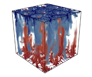
  $\operatorname {\mathit {Ra}}$, a columnar flow structure develops both in 2-D and in 3-D flows, as one can observe from the cross-section relative to the domain midheight in figure 1(a ii), while the near-wall region (figure 1a iii) is populated by thin filamentary plumes. This structure differs significantly from the classical RB turbulence, reported in figure 1(b), which is controlled in the bulk by large-scale rolls. In RB convection, large-scale structures span the entire domain, with typical length scales comparable to the height of the system. In comparison, in RD convection, columnar-like structures prevail, and are characterized by length scales distinct from the system's height. This difference will be taken into account when we build up a theory for RD convection in the following sections.

Figure 1. Instantaneous dimensionless temperature field  $T$ for convection in (a) porous media for $\operatorname {\mathit {Ra}}=10^4$, $W/L=1$ (Pirozzoli et al. Reference Pirozzoli, De Paoli, Zonta and Soldati2021), labelled as RD convection, and (b) in classical RB turbulence (thermal Rayleigh number $10^9$, Prandtl number $1$,
$1$,  $W/L=1$). The temperature distribution is shown over the entire volume (a i, b i), at the centreline $z=1/2$ (a ii, b ii) and near the upper wall (a iii, b iii).
Before presenting the dimensionless equations, we introduce the scaling quantities employed. The equations are made dimensionless with respect to convective flow scales (Pirozzoli et al. Reference Pirozzoli, De Paoli, Zonta and Soldati2021), namely, velocities are scaled with  $\mathcal {U}=\alpha g\Delta K/\nu$, where $\alpha$ is the thermal expansion rate, $\varDelta$ the temperature difference between the bottom and the top plate, $g$ the acceleration due to gravity, $\nu$ the kinematic viscosity and $K$ the permeability of the porous medium, which we assume to be homogeneous and isotropic. Lengths are scaled with $L$ and time with $\phi L/\mathcal {U}$. The dimensionless temperature is obtained as $T=(T^*-T^*_{top})/\varDelta$, with $T^*$ and $T^*_{top}$ the dimensional temperature field and the temperature value at the top boundary, respectively. Finally, pressure is scaled by $g L (\rho ^*_{top}-\rho ^*_{bot})$, where the top-to-bottom fluid density difference ( $\rho ^*_{top}-\rho ^*_{bot}$) is used. In an incompressible RD system, the heat transport is controlled by the dimensionless advection–diffusion equation (Pirozzoli et al. Reference Pirozzoli, De Paoli, Zonta and Soldati2021),
 \begin{equation} \frac{\partial T}{\partial t}+\boldsymbol{u}\boldsymbol{\cdot}\boldsymbol{\nabla} T=\frac{1}{\operatorname{\mathit{Ra}}}\nabla^2T { ,} \end{equation}
where  $\boldsymbol {u}$ and $T$ are the velocity and temperature fields, respectively, $t$ is time and $\operatorname {\mathit {Ra}}$ is the Rayleigh–Darcy number defined as
 \begin{equation} \operatorname{\mathit{Ra}}=\frac{\alpha g\Delta KL}{\kappa\nu}. \end{equation}
In this parameter, the medium ( $K$), domain ( $g,L$) and fluid ( $\alpha,\varDelta,\nu,\kappa$) properties are included, where $\kappa$ is the thermal diffusivity. The momentum transport and the flow incompressibility are accounted by the Darcy law and continuity equations,
 $$\begin{gather} \boldsymbol{u}={-}(\boldsymbol{\nabla} p-T\boldsymbol{k}), \end{gather}$$
 $$\begin{gather}\boldsymbol{\nabla}\boldsymbol{\cdot}\boldsymbol{u}=0, \end{gather}$$
respectively, where  $p$ is the reduced pressure field and $\boldsymbol {k}$ is the unit vector aligned with $z$.
$z$.
At the horizontal boundaries, we consider the temperature constant and equal to  $T=1$ at the bottom plate and $T=0$ at the top, so that an unstable configuration is achieved and the flow is driven by convection. No-penetration boundary conditions are assumed at both plates for the velocity, while the sides are considered periodic. Equations (2.1), (2.3) and (2.4) together with these boundary conditions determine the flow dynamics, which are controlled by two dimensionless parameters, namely $\operatorname {\mathit {Ra}}$ and the horizontal domain width $W/L$. The latter does not appear explicitly in the equations, but may play a significant role in determining the flow structure, especially at low $\operatorname {\mathit {Ra}}$.
3. Nusselt number and exact conservation equations
First, we will correlate the thermal (Nusselt number) and the kinetic (Péclet number) response parameters to the control parameter (Rayleigh–Darcy number), and then the thermal dissipation will be linked to the Nusselt number.
The temporal and horizontal average of (2.1) can be written as
 \begin{equation} \frac{\partial}{\partial z} \left ( \operatorname{\mathit{Ra}} \overline{\left \langle u_{z} T \right \rangle}_{A} - \overline{\left \langle \frac{\partial T}{\partial z} \right \rangle}_{A} \right ) = 0. \end{equation}
The Nusselt number then reads (Letelier, Mujica & Ortega Reference Letelier, Mujica and Ortega2019; Ulloa & Letelier Reference Ulloa and Letelier2022)
 \begin{equation} \operatorname{\mathit{Nu}}=\operatorname{\mathit{Ra}} \overline{\left\langle u_zT\right\rangle}_A-\overline{\left\langle \frac{\partial T}{\partial z} \right\rangle}_A. \end{equation}
Here the following notations are used for different averaging procedures. Overbars  $\overline {\cdots }$ correspond to the time average of a dimensionless value $f$, while an average over the horizontal surface and an average over the whole volume domain are denoted by $\langle \cdots \rangle _A$ and $\langle \cdots \rangle$,
 $$\begin{gather} \bar{f} = \frac{1}{\tau} \int_{t_0}^{t_0+\tau} f \,\mathrm{d} t, \end{gather}$$
 $$\begin{gather}\left \langle\, f \right \rangle_{A} = \frac{1}{A} \int_{0}^{W/L} \int_{0}^{W/L} f \,\mathrm{d}\kern 0.06em x \,\mathrm{d}y, \end{gather}$$
 $$\begin{gather}\left \langle\, f \right \rangle = \frac{1}{V} \int_{0}^{W/L} \int_{0}^{W/L} \int_{0}^{1} f \,\mathrm{d}\kern 0.06em x \,\mathrm{d}y \,\mathrm{d}z, \end{gather}$$
respectively, where  $A=(W/L)^2$ is the dimensionless horizontal surface area and $V=(W/L)^2$ is the dimensionless volume of the whole domain based on our characteristic length scale $L$. Two exact relations exist in our system and can be derived from the governing equations. Using the dimensionless velocity $\boldsymbol {u}$ to dot product both sides of (2.3) and combining with the incompressible continuity equation (2.4), we get
 \begin{equation} \left | \boldsymbol{u} \right |^2 ={-}\boldsymbol{\nabla}\boldsymbol{\cdot} (p\boldsymbol{u}) + Tu_z. \end{equation}
The volume and time average of (3.6) reads
 \begin{equation} \overline{\left\langle \left | \boldsymbol{u} \right |^2 \right\rangle} ={-}\frac{1}{V} \iint_{\varSigma} (p\boldsymbol{u}) \boldsymbol{\cdot} \hat{\boldsymbol{n}} \,\mathrm{d}S + \overline{\left\langle T u_z \right\rangle}, \end{equation}
where  $\varSigma$ is the boundary surface of the domain, $\mathrm {d}S$ denotes the surface element on the boundary and $\hat {\boldsymbol {n}}$ is the normal unit vector for the surface elements. The mean power given by the pressure gradient vanishes due to the non-penetration boundary condition,
 \begin{equation} \frac{1}{V} \iint_{\varSigma} (p\boldsymbol{u}) \boldsymbol{\cdot} \hat{\boldsymbol{n}} \,\mathrm{d}S ={-}\frac{1}{V} \iint_{\varSigma(z=0)} p u_z \,\mathrm{d}S + \frac{1}{V} \iint_{\varSigma(z=1)} p u_z \,\mathrm{d}S = 0. \end{equation}
The mean buoyancy power in (3.7) can be written as
 \begin{equation} \overline{\left\langle T u_z \right\rangle} = \frac{1}{V} \int_{0}^{1} \overline{\left \langle Tu_z \right \rangle}_A A \,\mathrm{d}z = \frac{1}{\operatorname{\mathit{Ra}}} \int_{0}^{1} \left (\operatorname{\mathit{Nu}} + \overline{\left\langle \frac{\partial T}{\partial z} \right\rangle}_A \right ) \mathrm{d}z. \end{equation}
Here, the last equivalence comes from the  $\operatorname {\mathit {Nu}}$ definition (3.2). Since we use $L$ as our length scale, $z\in [0,1]$. The last term in the above equation reads
 \begin{equation} \frac{1}{\operatorname{\mathit{Ra}}}\int_{0}^{1} \overline{\left\langle \frac{\partial T}{\partial z} \right\rangle}_A \,\mathrm{d}z = \frac{1}{\operatorname{\mathit{Ra}}}\int_{0}^{1} \frac{\partial \overline{\left\langle T \right\rangle}_A}{\partial z} \,\mathrm{d}z = \frac{1}{\operatorname{\mathit{Ra}}}\left ( \overline{\left\langle T \right\rangle}_A |_{z=1} - \overline{\left\langle T \right\rangle}_A |_{z=0} \right) ={-}\frac{1}{\operatorname{\mathit{Ra}}}. \end{equation}
Reintroducing (3.10) back into (3.9), after some algebraic manipulations we get
 \begin{equation} \overline{\left\langle T u_z \right\rangle} = \frac{1}{\operatorname{\mathit{Ra}}} \int_{0}^{1} \left (\operatorname{\mathit{Nu}} + \overline{\left\langle \frac{\partial T}{\partial z} \right\rangle}_A \right ) \mathrm{d}z = \frac{1}{\operatorname{\mathit{Ra}}} (\operatorname{\mathit{Nu}} - 1). \end{equation}
Combining (3.7), (3.8) and (3.11), we obtain an expression for the mean dimensionless velocity square,
 \begin{equation} \overline{\left\langle \left | \boldsymbol{u} \right |^2 \right\rangle} = \frac{1}{\operatorname{\mathit{Ra}}} (\operatorname{\mathit{Nu}} - 1). \end{equation}
We introduce the velocity scale
 \begin{equation} \mathcal{V} = \mathcal{U}\sqrt{\overline{\left \langle\left | \boldsymbol{u} \right |^2 \right\rangle}}, \end{equation}
with  $\mathcal {U}=\alpha g\Delta K/\nu$, and one finally obtains an exact relation
 \begin{equation} \operatorname{\mathit{Pe}}^2=(\operatorname{\mathit{Nu}}-1)\operatorname{\mathit{Ra}} \end{equation}
with
 \begin{equation} \operatorname{\mathit{Pe}} = \frac{\mathcal{V} L}{ \kappa} = \operatorname{\mathit{Ra}}\frac{\mathcal{V}}{\mathcal{U}}, \end{equation}
where  $\operatorname {\mathit {Pe}}$ is the Péclet number. The relation (3.14) aligns with the findings reported by Hassanzadeh et al. (Reference Hassanzadeh, Chini and Doering2014), albeit derived from a slightly different set of equations for porous media convection. Note that for RB convection, the analogous exact relation is $\epsilon _u=\nu ^3/L^4(\operatorname {\mathit {Nu}}-1)\operatorname {\mathit {Ra}}\operatorname {\mathit {Pr}}^{-2}$, where $\epsilon _u$ is the kinetic energy dissipation rate and $Pr$ is the Prandtl number (Ahlers et al. Reference Ahlers, Grossmann and Lohse2009). To assess the validity of (3.14), we consider the numerical measurements available in the literature. For 2-D flows, $\operatorname {\mathit {Pe}}$ is measured by De Paoli et al. (Reference De Paoli, Yerragolam, Lohse and Verzicco2024) using (3.13) and (3.15). The velocity root mean square (r.m.s.) at the centreline (2-D and 3-D) is computed by Hewitt et al. (Reference Hewitt, Neufeld and Lister2012, Reference Hewitt, Neufeld and Lister2014) and reported in figure 2(a).

Figure 2. (a) The r.m.s. of velocity used to estimate the Péclet number,  $\operatorname {\mathit {Pe}}$. Horizontal component ( ${\rm r.m.s.}(u)$), vertical component ( ${\rm r.m.s.}(w)$) and total (defined as $\sqrt {[{\rm r.m.s.}(u)]^2+[{\rm r.m.s.}(w)]^2}$ for 2-D cases, and $\sqrt {2[{\rm r.m.s.}(u)]^2+[{\rm r.m.s.}(w)]^2}$ for 3-D cases) are reported; data from Hewitt et al. (Reference Hewitt, Neufeld and Lister2012, Reference Hewitt, Neufeld and Lister2014). (b) Comparison of $\operatorname {\mathit {Pe}}$ compensated with $(\operatorname {\mathit {Nu}}-1)\operatorname {\mathit {Ra}}$ as from (3.14). Here $\operatorname {\mathit {Pe}}$ is computed with $\mathcal {V}$ defined as in (3.17) for the data from Hewitt et al. (Reference Hewitt, Neufeld and Lister2012, Reference Hewitt, Neufeld and Lister2014), and as in (3.13) for data from De Paoli et al. (Reference De Paoli, Yerragolam, Lohse and Verzicco2024). (c) Ratio of the Nusselt number to the dimensionless thermal dissipation, derived in (3.25); data from Pirozzoli et al. (Reference Pirozzoli, De Paoli, Zonta and Soldati2021) and De Paoli et al. (Reference De Paoli, Yerragolam, Lohse and Verzicco2024).
Since in all directions no mean flow exists, we have that  $\mathcal {V}$ is obtained from the r.m.s. of the velocity components ( $u_i$), namely
 \begin{equation} \mathcal{V} = \mathcal{U}\left(\overline{\left \langle[\text{r.m.s.}(u_x)]^2+[\text{r.m.s.}(u_y)]^2+[\text{r.m.s.}(u_z)]^2\right\rangle}\right)^{1/2}.\end{equation}
Assuming that the centreline flow is representative of the kinetic energy of the system, we have that
 \begin{equation} \mathcal{V} \approx\mathcal{U}\left(\overline{\left \langle[\text{r.m.s.}(u_x)]^2+[\text{r.m.s.}(u_y)]^2+[\text{r.m.s.}(u_z)]^2\right \rangle_{\varSigma(z=1/2)}}\right)^{1/2}. \end{equation}
We use this approximation to compute  $\mathcal {V}$ and verify the validity of (3.14) for the data of Hewitt et al. (Reference Hewitt, Neufeld and Lister2012, Reference Hewitt, Neufeld and Lister2014). We finally observe in figure 2(b) that (3.14) (dashed line) is in excellent agreement with the measurements obtained from the exact definition of $\operatorname {\mathit {Pe}}$ (2-D and $\mathcal {V}$ computed with (3.13) from De Paoli et al. (Reference De Paoli, Yerragolam, Lohse and Verzicco2024)) and also with measurements obtained from the approximated definition of $\operatorname {\mathit {Pe}}$ (2-D and 3-D, $\mathcal {V}$ computed with (3.17) from Hewitt et al. (Reference Hewitt, Neufeld and Lister2012, Reference Hewitt, Neufeld and Lister2014)).
We will now derive an equation to correlate the mean thermal dissipation to the Nusselt number. Multiplying the dimensionless thermal advection–diffusion equation (2.1) by  $T$, integrating over the whole domain and time-averaging, we have
 \begin{equation} \overline{\left \langle \frac{\partial}{\partial t} \left ( \frac{T^2}{2} \right ) \right \rangle} ={-} \overline{\left \langle T \boldsymbol{u} \boldsymbol{\cdot} \boldsymbol{\nabla} T \right\rangle} + \frac{1}{\operatorname{\mathit{Ra}}} \overline{\left \langle T \nabla^2 T \right\rangle}. \end{equation}
Under the assumption of a statistically steady state,
 \begin{equation} \overline{\left \langle \frac{\partial}{\partial t} \left ( \frac{T^2}{2} \right ) \right \rangle} = \frac{\partial}{\partial t} \overline{\left \langle \frac{T^2}{2} \right \rangle} = 0. \end{equation}
The first term on the right-hand side of (3.18) can be further written as
 \begin{equation} -\overline{\left \langle T \boldsymbol{u} \boldsymbol{\cdot}\boldsymbol{\nabla} T \right \rangle} = \overline{\left \langle \frac{T^2}{2} \boldsymbol{\nabla}\boldsymbol{\cdot}\boldsymbol{u} \right \rangle} - \overline{\left \langle \boldsymbol{\nabla}\boldsymbol{\cdot}\left ( \boldsymbol{u}\frac{T^2}{2} \right) \right \rangle} ={-}\frac{1}{V} \iint_{\varSigma} \left( \boldsymbol{u}\frac{T^2}{2} \right) \boldsymbol{\cdot} \hat{\boldsymbol{n}} \,\mathrm{d}S = 0. \end{equation}
Here we employed again continuity (2.4) and the no-penetration boundary condition. The second term on the right-hand side of (3.18) reads
 \begin{equation} \frac{1}{\operatorname{\mathit{Ra}}} \overline{\left \langle T \nabla^2 T \right\rangle} = \frac{1}{\operatorname{\mathit{Ra}}} \left[ \overline{\left \langle \nabla^2 \left( \frac{T^2}{2} \right) \right \rangle} - \overline{\left \langle \left\lvert \boldsymbol{\nabla} T \right\lvert^2 \right \rangle} \right]. \end{equation}
Combining results from (3.18)–(3.21), one obtains
 \begin{equation} \overline{\left \langle \left\lvert \boldsymbol{\nabla} T \right\lvert^2 \right \rangle} = \overline{\left \langle \nabla^2 \left( \frac{T^2}{2} \right) \right \rangle}. \end{equation}
We can use the following procedure to further simplify the right-hand side of (3.22):
 \begin{align} \overline{\left \langle \nabla^2 \left( \frac{T^2}{2} \right) \right \rangle} &= \frac{1}{V} \iint_{\varSigma} \left( \overline{T \boldsymbol{\nabla} T} \right) \boldsymbol{\cdot} \hat{\boldsymbol{n}} \,\mathrm{d}S \end{align}
 \begin{align} &= \frac{A}{V} \left ( \overline{\left\langle T\frac{\partial T}{\partial z} \right\rangle}_{\varSigma(z=1)} - \overline{\left\langle T\frac{\partial T}{\partial z} \right\rangle}_{\varSigma(z=0)} \right ) = \operatorname{\mathit{Nu}}. \end{align}
Here we considered that  $V=A=(W/L)^2$, applied the boundary conditions for $T$ and $u_z$, as well as the $\operatorname {\mathit {Nu}}$ definition (3.2). Combining (3.22) and (3.24), we get
 \begin{equation} \overline{\left \langle \left\lvert \boldsymbol{\nabla} T \right\lvert^2 \right \rangle} = \operatorname{\mathit{Nu}}, \end{equation}
where  $\overline { \langle \lvert \boldsymbol {\nabla } T \lvert ^2 \rangle }$ represents the dimensionless mean thermal dissipation. This relation, which holds also for RB convection (Ahlers et al. Reference Ahlers, Grossmann and Lohse2009), has been also presented before for RD flows (Otero et al. Reference Otero, Dontcheva, Johnston, Worthing, Kurganov, Petrova and Doering2004; Hidalgo et al. Reference Hidalgo, Fe, Cueto-Felgueroso and Juanes2012; De Paoli Reference De Paoli2023) and for Hele-Shaw convection the limit of infinitely thin domains (Letelier et al. Reference Letelier, Mujica and Ortega2019; Ulloa & Letelier Reference Ulloa and Letelier2022). The ratio of the Nusselt number to the dimensionless thermal dissipation is compared in figure 2(c) for the numerical results of Pirozzoli et al. (Reference Pirozzoli, De Paoli, Zonta and Soldati2021) and De Paoli et al. (Reference De Paoli, Yerragolam, Lohse and Verzicco2024). We observe that, also in this case, the agreement between theory and simulations is good, confirming the validity of (3.25). Finally, one obtains the dimensional thermal dissipation rate,
 \begin{equation} \epsilon=\kappa\frac{\varDelta^2}{L^2} \overline{\left \langle \left\lvert \boldsymbol{\nabla} T \right\lvert^2 \right \rangle} = \kappa\frac{\varDelta^2}{L^2} \operatorname{\mathit{Nu}}. \end{equation}
Equations (3.14) and (3.26) represent the two exact relations we derived in our system.
4. Application of GL theory and scaling relation for the Nusselt number
With the two exact relations derived in the previous section, we can now apply the main ideas of the GL theory to RD convection. The key idea of the GL theory (Grossmann & Lohse Reference Grossmann and Lohse2000, Reference Grossmann and Lohse2001) is to split the kinetic and thermal dissipation rates into contributions from the BLs and bulk. In RD convection, the procedure becomes even simpler than in RB, as only the thermal dissipation rate appears in the exact relations. We separate the mean thermal dissipation as
 \begin{equation} \epsilon=\epsilon_{BL}+\epsilon_{bulk}, \end{equation}
and apply the respective scaling relations for  $\epsilon _{BL}$ and $\epsilon _{bulk}$, based on the BL theory and fully developed flow in the bulk. The horizontal- and time-averaged profiles of temperature, shown in figure 3(a), confirm that the flow can be split into two distinct regions: a well-mixed bulk with nearly uniform properties, and a thin BL characterized by a linear temperature profile, the slope of which is unitary when $z$ is rescaled with $\operatorname {\mathit {Nu}}$ (figure 3b). The thickness of this BL, $\lambda /L$, can be determined as the distance from the wall at which the linear function fitting the temperature profile in the bulk ( $0.4\leqslant z \leqslant 0.6$) intersects the near-wall temperature fit. The measurement procedure is illustrated in figure 3(c), where the intersection is marked by the bullet. The Nusselt number sets the thickness of the BL $\lambda /L =1/(2\operatorname {\mathit {Nu}})$ (De Paoli et al. Reference De Paoli, Pirozzoli, Zonta and Soldati2022). In RD convection, it has been proposed by Otero et al. (Reference Otero, Dontcheva, Johnston, Worthing, Kurganov, Petrova and Doering2004) that the thermal BL thickness scales as $\lambda /L \sim \operatorname {\mathit {Ra}}^{-1}$ (consistent with $Nu \sim Ra$, from the classical theory (Malkus Reference Malkus1954; Priestley Reference Priestley1954; Howard Reference Howard1966) and the upper bound scaling derived by Doering & Constantin (Reference Doering and Constantin1998)). As illustrated in figure 3(d), this approximation is verified. Although both in 2-D and 3-D cases the thermal BL thickness follows $\lambda /L \sim \operatorname {\mathit {Ra}}^{-1}$, the prefactor differs (see figure 3d). This discrepancy arises from the distinct flow structures in 2-D and 3-D cases. In 3-D cases, owing to the additional degree of freedom compared with the 2-D case, plumes can freely move and reorganize towards the most efficient configuration, resulting in a different value of $\operatorname {\mathit {Nu}}$. Consequently, the BL thickness also varies. This phenomenon is analogous to RB convection, where 2-D and 3-D flows exhibit different BL thicknesses due to variations in $\operatorname {\mathit {Nu}}$ (Van Der Poel, Stevens & Lohse Reference Van Der Poel, Stevens and Lohse2013).

Figure 3. (a) Horizontal- and time-averaged profiles of temperature are shown for different  $\operatorname {\mathit {Ra}}$ (De Paoli et al. Reference De Paoli, Pirozzoli, Zonta and Soldati2022). The near-wall region is magnified in (b), where the wall-normal coordinate is rescaled with $\operatorname {\mathit {Nu}}$. The profiles are self-similar, and in the BL follow a linear behaviour (solid line) with unitary slope. (c) The thickness of the BL is determined as the distance from the wall of the intersection between the linear profile fitting the bulk ( $0.4\leqslant z \leqslant 0.6$) and the near-wall regions ( $z\le 0.1\operatorname {\mathit {Nu}}/\operatorname {\mathit {Ra}}$). The case relative to $\operatorname {\mathit {Ra}}=10^4$ is reported. A close-up view of the near-wall region is shown in the inset. (d) Thickness of the thermal BL $\lambda /L$ as a function of the Rayleigh number. The 3-D measurements computed as discussed (bullets) are very well fitted by the correlation $50/\operatorname {\mathit {Ra}}$. The correlation proposed for 2-D flows by Otero et al. (Reference Otero, Dontcheva, Johnston, Worthing, Kurganov, Petrova and Doering2004) ( $\lambda /L\sim 15/\operatorname {\mathit {Ra}}$) is also reported, as well as the value obtained from the Nusselt number $\lambda /L=1/(2\operatorname {\mathit {Nu}})$; data from De Paoli et al. (Reference De Paoli, Pirozzoli, Zonta and Soldati2022).
The profiles of dimensionless thermal dissipation  $\overline {\langle |\boldsymbol {\nabla } T|^2\rangle _A}$ obtained from De Paoli et al. (Reference De Paoli, Pirozzoli, Zonta and Soldati2022) are shown in figure 4(a) for different values of the Rayleigh number. In the inset, the dissipation is rescaled by the respective Nusselt number, and shown up to 1. We observe that the BL contribution to the dissipation is more pronounced as $\operatorname {\mathit {Ra}}$ is increased. A more quantitative description is provided in the following. The thermal dissipation rate in the BL scales as $\sim \kappa (\varDelta /\lambda )^2$. Therefore, taking into account the layer extension ( $\lambda /L\sim \operatorname {\mathit {Ra}}^{-1}$), the BL contribution towards the total thermal dissipation rate reads
 \begin{equation} \epsilon_{BL}\sim\kappa\frac{\varDelta^2}{\lambda^2}\frac{\lambda}{L}\sim\kappa\frac{\varDelta^2}{L^2}\operatorname{\mathit{Ra}}. \end{equation}
Assuming the flow in the bulk is well mixed (Grossmann & Lohse Reference Grossmann and Lohse2000; Bader & Zhu Reference Bader and Zhu2023; Song, Shishkina & Zhu Reference Song, Shishkina and Zhu2024), we get
 \begin{equation} \epsilon_{bulk}\sim\frac{\mathcal{V}\theta^2}{\ell}. \end{equation}
Here,  $\mathcal {V}$ and $\theta$ are the typical velocity and temperature scales, respectively. The characteristic length scale is $\ell$, defined as the wavelength associated with the power-averaged mean wavenumber at the midheight $(\bar {k})$, i.e. $\ell /L=2{\rm \pi} /\bar {k}$. In numerical simulations, $\bar {k}$ is obtained from the time-averaged spectrum of the temperature field at $z=1/2$ (Hewitt et al. Reference Hewitt, Neufeld and Lister2014). The importance of $\epsilon _{BL}$ and $\epsilon _{bulk}$ relative to the total dissipation $\epsilon$, is reported in figure 4(b) for 3-D RD convection (De Paoli et al. Reference De Paoli, Pirozzoli, Zonta and Soldati2022). Here, $\epsilon _{BL}$ and $\epsilon _{bulk}$ are obtained from the profiles, and represent the mean value within the respective regions. In RB, to derive the scalings, the length scale is assumed to be the height of the domain $L$, which makes sense as there exist large-scale rolls. However, here in RD, the typical flow structures are columnar-like, making the length scale $\ell$ different from $L$. This difference is clearly visible in figures 1(a i) and 1(b i). From the definition of $\operatorname {\mathit {Nu}}$ (3.2) and assuming that in the bulk, $\theta \sim \operatorname {\mathit {Nu}}(\kappa \varDelta )/(\mathcal {V}L)$, and when $\operatorname {\mathit {Nu}}$ only comes from the fluctuation in the bulk, $\theta \sim (\epsilon _{bulk}/\mathcal {V})( L/\varDelta )$, we get
 \begin{equation} \epsilon_{bulk}\sim\kappa\frac{\varDelta^2}{L^2}{\operatorname{\mathit{Pe}}}\frac{\ell}{L}. \end{equation}
The same bulk scaling has also been reported for rapidly rotating convection (Song et al. Reference Song, Shishkina and Zhu2024) and magnetoconvection with strong vertical magnetic fields (Bader & Zhu Reference Bader and Zhu2023). In all these three systems, in the bulk there exists a new horizontal dominant length scale that is different from the height of the domain. In each of these three systems, a new dominant length scale emerges, distinct from the domain's height. This disparity constitutes a significant deviation from the original GL theory.
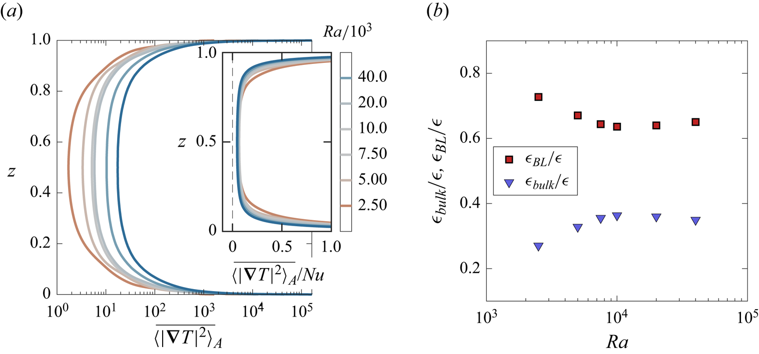
Figure 4. (a) Horizontal- and time-averaged profiles of dimensionless thermal dissipation,  $\overline {\langle |\boldsymbol {\nabla } T|^2\rangle _A}$, are shown for different $\operatorname {\mathit {Ra}}$ (De Paoli et al. Reference De Paoli, Pirozzoli, Zonta and Soldati2022). In the inset, the dissipation is rescaled by the respective Nusselt number, and shown up to $\overline {\langle |\boldsymbol {\nabla } T|^2\rangle _A}/\operatorname {\mathit {Nu}}=1$. The BL contribution to the dissipation is more pronounced as $\operatorname {\mathit {Ra}}$ is increased. (b) Contributions to the mean scalar dissipation $\epsilon$ within the BL ( $\epsilon _{BL}$) and in the bulk region ( $\epsilon _{bulk}$); data are from De Paoli et al. (Reference De Paoli, Pirozzoli, Zonta and Soldati2022).
Determining the dominant wavelength in RD convection is a challenging task. The reason is linked to the complex way in which the dynamic near-wall flow structures interact with the stationary, large-scale columnar plumes controlling the bulk. A detailed review is provided by Hewitt (Reference Hewitt2020), which we summarize here with additional details including later results (De Paoli et al. Reference De Paoli, Pirozzoli, Zonta and Soldati2022). In 3-D cases, using asymptotic stability theory, Hewitt & Lister (Reference Hewitt and Lister2017) derived that
 \begin{equation} \ell/L\sim \operatorname{\mathit{Ra}}^{{-}1/2} \quad {\rm (3}\hbox{-}{\rm D)}. \end{equation}
Numerical simulations by Hewitt et al. (Reference Hewitt, Neufeld and Lister2014) and De Paoli et al. (Reference De Paoli, Pirozzoli, Zonta and Soldati2022), best fitted by scaling exponents of  $-0.52$ and $-0.49$, respectively, agree well with this prediction (see also figure 5a). Therefore, we employ this scaling relation ( $\ell /L\sim \operatorname {\mathit {Ra}}^{-1/2}$) for the centreline in 3-D cases. The situation is more complex in 2-D cases. Hewitt, Neufeld & Lister (Reference Hewitt, Neufeld and Lister2013b) derived analytically the scaling relation
 \begin{equation} \ell/L\sim \operatorname{\mathit{Ra}}^{{-}5/14} \quad {\rm (2}\hbox{-}{\rm D)}. \end{equation}
Wen, Corson & Chini (Reference Wen, Corson and Chini2015) have shown that for  $\operatorname {\mathit {Ra}}\le 19\,976$ the centreline dominant length scale is well approximated by $\ell /L\sim \operatorname {\mathit {Ra}}^{-0.40}$. However, one can observe in figure 5(b) that when $\operatorname {\mathit {Ra}}\ge 39\,716$, the interplume spacing measured by Wen et al. (Reference Wen, Corson and Chini2015) is not unique. The conclusion is that in 2-D RD convection, at $\operatorname {\mathit {Ra}}\ge 39\,716$, a precise scaling remains to be established by running simulations in very wide domains and for very long times. In view of this, we consider the scaling proposed by Hewitt et al. (Reference Hewitt, Neufeld and Lister2013b), which represents the best theoretical prediction available, to be valid. Therefore, combining (4.4) with (3.14), (4.5) and (4.6), we get
 \begin{equation} \epsilon_{bulk}\sim\kappa\frac{\varDelta^2}{L^2}\operatorname{\mathit{Nu}}^{1/2} \quad {\rm (3}\hbox{-}{\rm D)}, \end{equation}
and
 \begin{equation} \epsilon_{bulk}\sim\kappa\frac{\varDelta^2}{L^2}{\operatorname{\mathit{Nu}}^{1/2}\operatorname{\mathit{Ra}}^{1/7}} \quad {\rm (2}\hbox{-}{\rm D)}. \end{equation}
Figure 5. Dominant length scales  $\ell /L$ in the bulk ( $z=1/2$) for (a) 3-D (Hewitt et al. Reference Hewitt, Neufeld and Lister2014; De Paoli et al. Reference De Paoli, Pirozzoli, Zonta and Soldati2022) and (b) 2-D (Hewitt et al. Reference Hewitt, Neufeld and Lister2012; Wen et al. Reference Wen, Corson and Chini2015) simulations. Theoretical scaling relations defined in (4.5) and (4.6), corresponding to 3-D and 2-D flows, respectively, are also indicated (dashed lines).
Finally, combining (3.26), (4.1), (4.2), (4.7) and (4.8), we reach an expression for  $\operatorname {\mathit {Nu}}$ as a function of $\operatorname {\mathit {Ra}}$ for the 3-D and the 2-D cases, as follows:
 $$\begin{gather} \operatorname{\mathit{Nu}}=A_3\operatorname{\mathit{Ra}}+B_3\operatorname{\mathit{Nu}}^{1/2} \quad {\rm (3}\hbox{-}{\rm D)}, \end{gather}$$
 $$\begin{gather}\operatorname{\mathit{Nu}}=A_2\operatorname{\mathit{Ra}}+B_2\operatorname{\mathit{Nu}}^{1/2}\operatorname{\mathit{Ra}}^{1/7} \quad {\rm (2}\hbox{-}{\rm D)}. \end{gather}$$
As reported in figure 6, these scaling relations fit very well the data obtained from numerical simulations, both in the 2-D and in the 3-D cases. The values of the coefficients  $A_2$, $A_3$, $B_2$, $B_3$, indicated in figure 6, are obtained as best fitting from the data shown, representing the numerical results available and with $\operatorname {\mathit {Ra}}>2\times 10^3$. The choice of considering values larger than this threshold is motivated by the flow topology: at low $\operatorname {\mathit {Ra}}$ the bulk flow structure is not columnar, as it is dominated by large-scale convective rolls (Graham & Steen Reference Graham and Steen1994), and therefore our theory does not apply. The expressions of $\operatorname {\mathit {Nu}}$ derived in (4.9) and (4.10) take the form of a linear scaling with a sublinear correction. The linear scaling was previously proposed for 2-D (Hewitt et al. Reference Hewitt, Neufeld and Lister2012) and 3-D (Hewitt et al. Reference Hewitt, Neufeld and Lister2014) flows. The scaling proposed here provides similar results to the linear scaling with sublinear corrections proposed for the 3-D case by Pirozzoli et al. (Reference Pirozzoli, De Paoli, Zonta and Soldati2021). However, in this case one fitting parameters fewer is used, i.e. all scaling exponents are known. The good agreement of the present scaling relations with the numerical measurements available in the literature suggests that the theory proposed is indeed valid and promising for higher $\operatorname {\mathit {Ra}}$. The RD system is completely defined by two parameters, namely the Rayleigh number $\operatorname {\mathit {Ra}}$ and the aspect ratio $W/L$. In 3-D flows at high- $\operatorname {\mathit {Ra}}$, it has been observed that all major flow statistics converge for an aspect ratio of $W/L=1$ (De Paoli et al. Reference De Paoli, Pirozzoli, Zonta and Soldati2022). This differs in 2-D systems: also at high $\operatorname {\mathit {Ra}}$ and due to the additional lateral confinement, the aspect ratio may have an influence on $\ell$ (Wen et al. Reference Wen, Corson and Chini2015). Therefore, it may be required to take $W/L$ into account in the present theory to better describe the transport properties in 2-D RD flows. To this aim and also to assess the physics of the scaling prefactors, additional simulations in large domains and at larger $\operatorname {\mathit {Ra}}$ are needed.

Figure 6. Compensated Nusselt number as a function of Rayleigh number. Results are for 2-D (Hewitt et al. Reference Hewitt, Neufeld and Lister2012; Wen et al. Reference Wen, Corson and Chini2015; De Paoli, Zonta & Soldati Reference De Paoli, Zonta and Soldati2016; Pirozzoli et al. Reference Pirozzoli, De Paoli, Zonta and Soldati2021; De Paoli et al. Reference De Paoli, Yerragolam, Lohse and Verzicco2024) and 3-D (Hewitt et al. Reference Hewitt, Neufeld and Lister2014; Pirozzoli et al. Reference Pirozzoli, De Paoli, Zonta and Soldati2021) simulations. New fitting curves are obtained considering all data with  $\operatorname {\mathit {Ra}}>2\times 10^3$, with numerical values of the coefficients being $A_2 = (6.386 \pm 0.007)\times 10^{-3}$, $B_2=0.2533\pm 0.0050$ and $A_3 = (8.592 \pm 0.033)\times 10^{-3}$, $B_3=1.376\pm 0.059$. The coefficients of determination ( $R^2$) for the best fitting curves provided are 0.991 and 0.999 in the 2-D and in the 3-D cases, respectively.
5. Conclusions
In summary, we have established two exact relationships, one pertaining to the Péclet number and the other to the thermal dissipation rate, in the context of Rayleigh–Darcy (RD) convection – a fundamental system for heat and mass transport in porous media. Inspired by previous models developed for RB convection (Grossmann & Lohse Reference Grossmann and Lohse2000, Reference Grossmann and Lohse2001), we have formulated a scaling theory for heat transfer in 2-D and 3-D RD flows, where the Nusselt number is expressed as a function of the Rayleigh number as described by (4.9) and (4.10). This theory enables us to provide a theoretical explanation to the sublinear empirical corrections proposed in prior studies (Pirozzoli et al. Reference Pirozzoli, De Paoli, Zonta and Soldati2021). Our investigations, supported by both the 2-D and 3-D literature results, confirm the validity of the proposed theory. Moreover, by taking the length scale of the flow structures into account, we also shed new light on the physical origins of the disparities in scaling relations between 2-D and 3-D RD convection.
Our findings are relevant to convective flows in homogeneous and isotropic porous media where the top-to-bottom density difference is defined. However, these hypotheses represent idealized conditions not taking into account additional flow features that occur in realistic processes, such as hydrodynamic dispersion (Liang et al. Reference Liang, Wen, Hesse and DiCarlo2018; Tsinober et al. Reference Tsinober, Rosenzweig, Class, Helmig and Shavit2022; Tsinober, Shavit & Rosenzweig Reference Tsinober, Shavit and Rosenzweig2023), medium heterogeneity (Simmons, Fenstemaker & Sharp Reference Simmons, Fenstemaker and Sharp2001; Dentz, Hidalgo & Lester Reference Dentz, Hidalgo and Lester2023), anisotropy (Ennis-King, Preston & Paterson Reference Ennis-King, Preston and Paterson2005; De Paoli et al. Reference De Paoli, Zonta and Soldati2016) and alternative flow configurations (Hidalgo et al. Reference Hidalgo, Fe, Cueto-Felgueroso and Juanes2012; De Paoli, Zonta & Soldati Reference De Paoli, Zonta and Soldati2017; Letelier et al. Reference Letelier, Ulloa, Leyrer and Ortega2023). Nonetheless, present findings represent a crucial step required to develop a robust and physically sound theory for convection in porous media flows, which can be further expanded to include the presence of the different variations mentioned above. We consider for instance the sequestration of carbon dioxide in saline aquifers. Such a system is usually modelled as a rectangular domain initially filled with brine and confined by two horizontal low-permeability layers, and therefore it is assumed to be impermeable at the bottom boundary (no-flux) (Huppert & Neufeld Reference Huppert and Neufeld2014). Here, the solute enters from the top, in correspondence of which the concentration of  ${\rm CO}_2$ is constant. This flow configuration, defined as ‘one-sided’ (Hewitt, Neufeld & Lister Reference Hewitt, Neufeld and Lister2013a) or ‘semi-infinite’ (Ennis-King et al. Reference Ennis-King, Preston and Paterson2005), is subject to a transient behaviour: the average ${\rm CO}_2$ concentration within the system will increase over time, and it will be progressively harder to keep dissolving solute. In quantitative terms this means that, after a short initial phase in which dissolution increases due to the formation and growth of the fingers, the flux of solute through the top boundary will later reduce as a result of the saturation of the domain. The dynamics of such a system has been thoroughly characterized (Slim Reference Slim2014), and it is shown to be quantitatively related to the dynamics observed in RD convection (Hewitt et al. Reference Hewitt, Neufeld and Lister2013a; De Paoli et al. Reference De Paoli, Zonta and Soldati2017). In order to describe the evolution of the one-sided system with a simple box-model, accurate predictions of the transport scaling in RD convection are essential. In the presence of high-permeability formations such as the Utsira Sand reservoir at Sleipner (Bickle et al. Reference Bickle, Chadwick, Huppert, Hallworth and Lyle2007), the Rayleigh–Darcy number may be as high as $6\times 10^5$ (Hewitt et al. Reference Hewitt, Neufeld and Lister2013a), which is beyond current numerical capabilities. As a result, the theoretical results provided in our work will play a crucial role as a tool to determine the long-term evolution of flows in semi-infinite domains.
Funding
We gratefully acknowledge the financial support from the Max Planck Society, the German Research Foundation through grants 521319293 and 540422505, the Alexander von Humboldt Foundation and the Daimler Benz Foundation. This project has also received funding from the European Union's Horizon Europe research and innovation programme under the Marie Sklodowska–Curie grant agreement no. 101062123.
Declaration of interests
The authors report no conflict of interest.


 Open access